3.1 Training set generation

Our neural network approach to the retrieval of cloud properties from POLDER-3 data decomposes the retrieval task into four subtasks, with a different neural network dedicated to each. A first level of separation was made between retrievals over land and over ocean. Second, separate neural networks were trained for the estimation of the COT and for the estimation of cloud microphysical properties (effective radius and effective variance). Having separate NNs specialized on cloud retrievals above ocean and land is expected to simplify the training of each NN. The separation between COT and microphysical properties retrievals was made because, given the physical nature of the retrieval problem, a different measurement vector appears more suitable for each of these two retrievals. The information on COT is especially present in radiance, with polarization bringing additional information for small optical thicknesses. Since POLDER did not have spectral channels with significant absorption by liquid water, information about cloud droplet size in POLDER measurements is only contained in the angular and spectral dependence of polarized radiance in the cloudbow region. For this reason, our NN scheme for COT retrieval uses multi-angle and multi-wavelength radiance and degree of linear polarization (DoLP) measurements, whereas the NN for the effective radius and effective variance retrievals only relies on multi-angle and multi-wavelength polarized radiance measurements. Furthermore, effective radius and effective variance retrievals are only performed if the scattering angle range at which measurements are performed includes the cloudbow range of 135 to 165^∘, whereas this restriction does not apply to COT retrievals. An additional differentiation between the neural network for COT retrieval over ocean and that for COT retrieval over land concerns the measurement vector used in the retrieval. The ocean neural network uses reflectances at 490, 675, 860 and 1020 nm and DoLPs at 490, 675 and 860 nm as inputs, whereas the land network does not make use of the wavelengths 860 and 1020 nm in order to avoid dealing with the large variability in the reflective properties of land surfaces at these wavelengths. The reflectance at 565 nm is used as an additional input in the NN for COT retrieval over land.

The NNs presented in this study have been trained using synthetic data. While the prior distributions of the cloud properties used to generate the training sets are the same for all the NNs, a difference lies in the treatment of the surface properties between the ocean networks and the land networks. In the radiative transfer simulations produced in order to train the ocean network, the surface properties are parameterized with respect to wind speed as in Cox and Munk (1954), to chlorophyll concentration as in Morel and Maritorena (2001) and Chowdhary et al. (2006), and to whitecap fraction and foam albedo as in Koepke (1984). For the land network, instead, the surface bidirectional reflectance distribution function (BRDF) has been parameterized using the Ross–Li model (Maignan et al., 2004, and references therein), and the bidirectional polarization distribution function (BPDF) has been parameterized as in Maignan et al. (2009). For both land and ocean simulations, the radiative transfer model described in Hasekamp and Landgraf (2002, 2005) has been used. Clouds have been parameterized as spherical particles with a Gamma size distribution, with a refractive index taken from the Optical Properties of Aerosols and Clouds (OPAC) database (Hess et al., 1998). In order to reduce the computational complexity of the radiative transfer simulations, the forward scattering peak in the phase function of cloud droplets has been accounted for by means of the “MS correction” proposed by Nakajima and Tanaka (1988).

An important aspect to be pointed out, which may represent a limitation in our approach, is that the often highly peaked phase functions of cloud droplets make it important to use an adequate number of streams in the forward model calculations. For example, in Fig. 1 a plot is shown of the simulated top-of-atmosphere (TOA) reflectance at 443.9 nm versus COT for 8, 16, 32 and 64 streams, assuming spherical cloud particles and a Gamma size distribution with an effective radius of 25 µm and an effective variance of 0.03. The simulations were performed for a solar zenith angle of 30^∘ and assuming nadir observation. It can be seen that, for COT larger than approximately 20, the simulated TOA reflectances critically depend on the chosen number of streams. A higher number of streams generally results in more accurate radiative transfer simulations but also leads to an increased computation time. Since the generation of our neural network training dataset involves a large number of radiative transfer simulations (of the order of 10⁵ to 10⁶), we were forced to limit the number of streams to 16 even if this does not appear to be the most accurate choice, as choosing a higher number of streams would have led to overly time-consuming simulations.

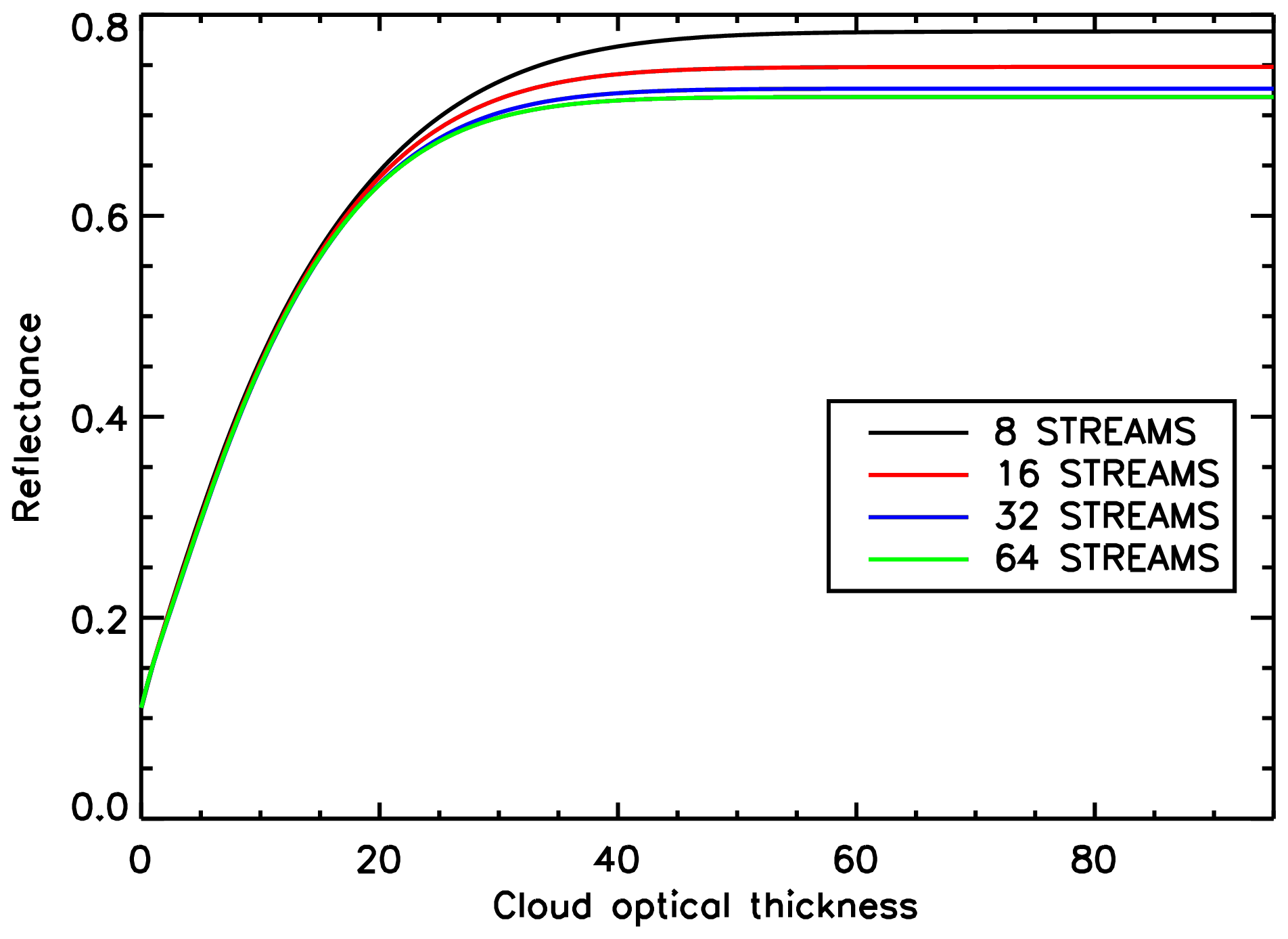
Figure 1Dependence of simulated TOA reflectance at 443.9 nm on the number of streams used in the radiative transfer calculations.

Download

An additional limitation – not specific to our approach but caused by the 1-D homogeneous cloud assumption (Zhang and Platnick, 2011) – is that reflectance measurements in the optical range saturate for COTs larger than ∼40. This means that not enough information is available to distinguish COTs around this value from larger COTs. For this reason, we decided to use a maximum COT of 40 in the generation of the training datasets for our four neural networks.

As pointed out in Sect. 1, a very important element in the design of a neural network algorithm dealing with multi-angle large-swath measurements is how to deal with the variability in the set of viewing angles at which the measurements are performed. Our approach is similar to that proposed by Han et al. (2006) in the context of aerosol retrievals from the Multi-angle Imaging SpectroRadiometer (MISR) and basically consists of using the set of viewing angles as additional input quantities for the neural network. However, a difference between the two approaches lies in the way the neural networks are trained. While Han et al. (2006) trained their neural network scheme using real MISR measurements co-located with MODIS Level 2 aerosol properties, our neural networks are trained on synthetic data. In order to perform our simulations at viewing angle combinations representative of actual POLDER-3 measurements, we sampled 1 year of POLDER-3 measurements, randomly selecting 25 orbits per month and 5000 combinations of viewing zenith angles, solar zenith angles and relative azimuth angles per orbit. We thereby generated a database of 1.5×10⁶ angle combinations which we used as inputs for our radiative transfer calculations. Since the number of angles at which POLDER-3 performed its measurements is also variable, we decided to only consider measurements performed at a minimum of 14 angles to train our neural networks. This number was chosen in order to have a good trade-off between the benefit of having a good number of available viewing angles and that of not discarding too many measurements, as would have been the case if we only considered measurements performed at 16 angles (the maximum available number for POLDER-3). Also for POLDER-3 measurements performed at more than 14 angles, only 14 angles are used in the input vector for the neural networks. This choice was made in order to avoid dealing with the difficulty of having a input vector of variable size or, as an alternative, of passing input vectors with missing data to the neural networks.

Table 1List of input quantities used in the COT neural network and in the effective radius neural network. The check mark (✓) indicates that a given quantity (or set of quantities) is used in a neural network.

Download Print Version | Download XLSX

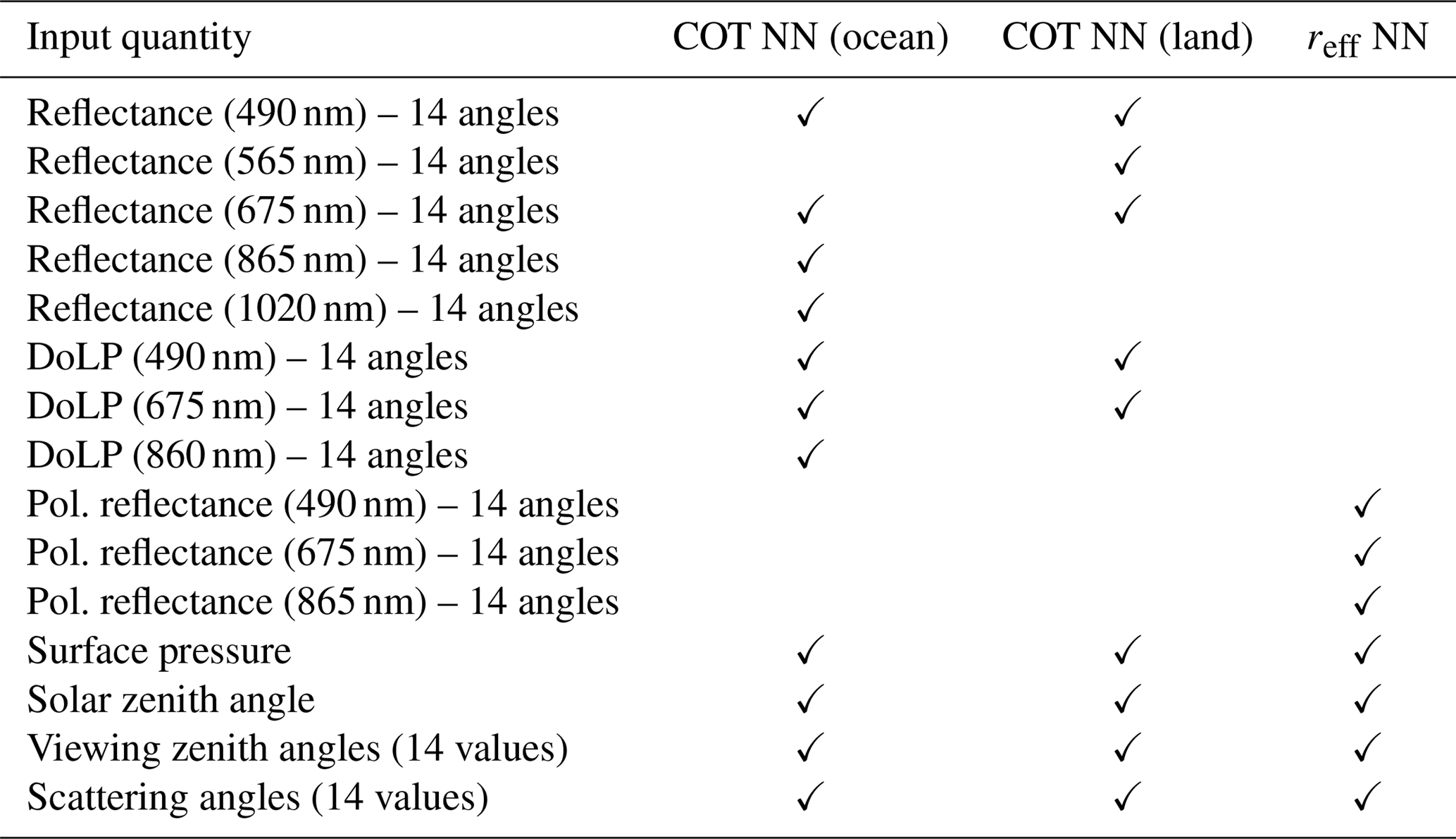
As discussed at the beginning of this section, the quantities used in the input vector differ between the COT retrieval neural networks and the effective radius retrieval neural networks. The complete list of input quantities for each network is given in Table 1. Effective variance is retrieved as an additional parameter in the effective radius network, whereas cloud top height is retrieved as an additional parameter in both networks. The ocean and land surface parameters are not included in the output vector but are randomized in the training set. From a theoretical standpoint, this corresponds to designing a neural network that approximates the conditional expectation of the set of cloud properties x given the measurement vector y, marginalized over the possible values of the surface properties. Mathematically, if we introduce a vector b describing the surface properties, the neural network will return an approximation of the following conditional expectation:

where f_b is the probability density function of b and 𝒟 is the domain of f_b. The same logic was followed in the treatment of cloud microphysical parameters in the COT retrieval NN and of COT in the microphysical parameter retrieval NN, i.e. rather than making an assumption about the non-retrieved parameters and keeping them constant in the training set, they are randomized. This approach enables the training procedure to adjust the weights of the NN based on the input features that are of direct relevance for the retrieval of the parameter at hand, preventing biases due to incorrect assumptions. A “classical” equivalent of this approach would consist of averaging multiple retrievals carried out using different assumptions.

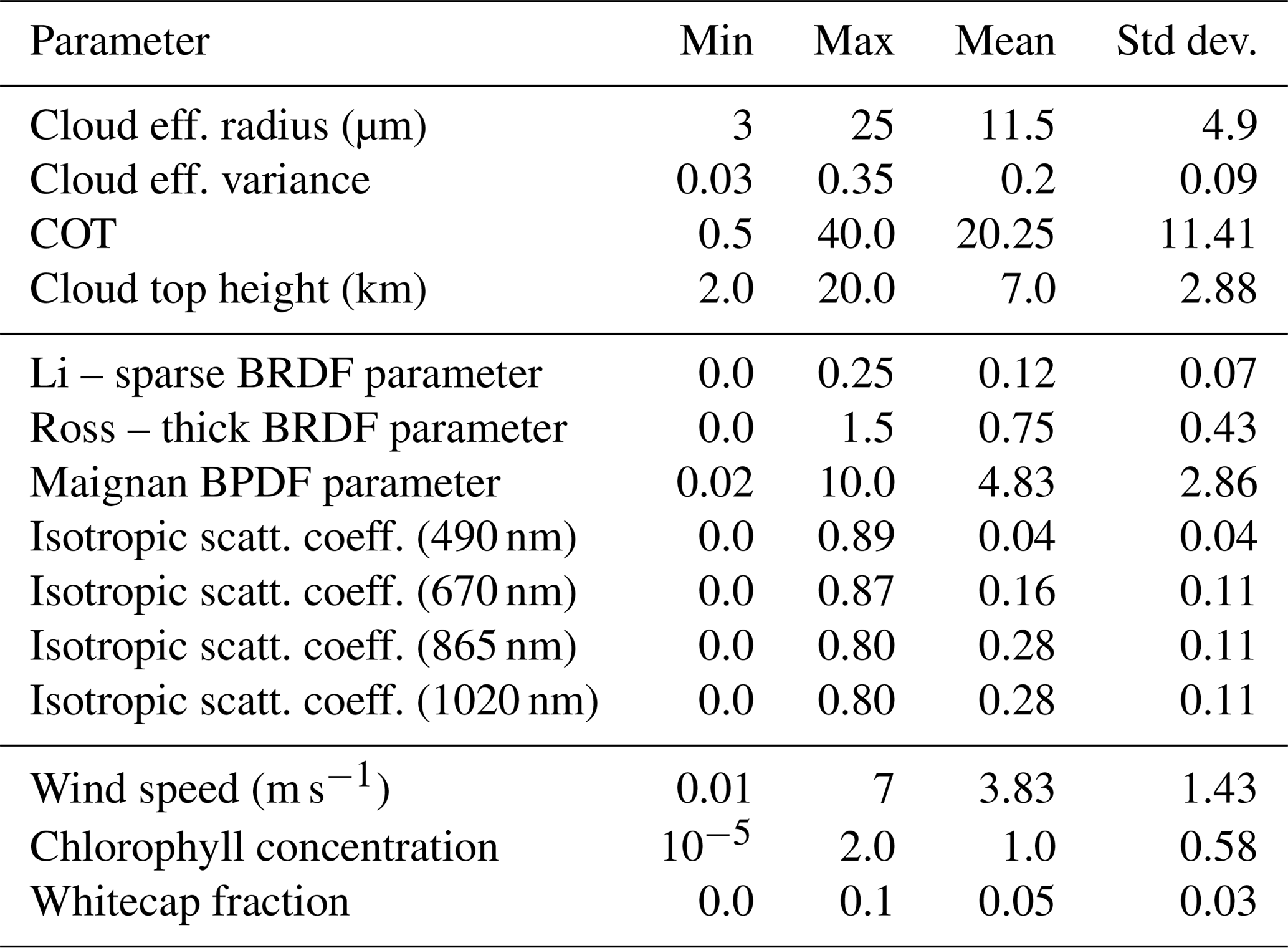
The details of statistical distributions of the cloud, ocean and land surface parameters used in the radiative transfer simulations are summarized in Table 2.

The measurement noise was modelled as an additive Gaussian random variable with a zero mean and a standard deviation of 1 % for reflectance, 2 % for polarized reflectance and 0.7 % for DoLP. As done in previous work (Di Noia et al., 2015, 2017), such noise was added to the synthetic measurements during the training phase as a form of regularization, as explained in Bishop (1995). The neural network architecture was chosen based on results inherited from previous work and, for all the four networks, consists of three hidden layers with 40 neurons each.

Table 2Details of the statistical distributions of the cloud and surface parameters used to generate the training datasets.

Download Print Version | Download XLSX

3.2 The ensemble approach

As anticipated in Sect. 1, training a neural network to invert multi-angular measurements from a large-swath instrument is a difficult task. In an attempt to reduce the retrieval uncertainty caused by imperfect training, we decided to train multiple neural networks and use the average of their outputs as our final retrieval. This approach – called the “neural network ensemble” approach (Hansen and Salamon, 1990) – is known to reduce the random component of the neural network output error and has been already applied with success in remote sensing contexts (Krasnopolsky, 2007). In principle, several methods exist to combine the results of multiple neural networks in order to build an enhanced estimator, and an overview of such methods is given by Sharkey (1996). In this work, we have chosen to train multiple neural networks characterized by the same architecture and on the same training set, varying the random initial value of the neural network weights. In practice, in this way, each ensemble member (i.e. each individual net) is trained so that its weight vector approaches a different local minimum of the error surface (Tresp, 2002). It is possible to prove that this method ensures that the variance of the error of the neural network ensemble is smaller than the average variance of the single ensemble members (Perrone, 1993). Contrary to the error variance, the bias is not reduced by the ensemble approach.

The maximum reduction in variance is achieved when the errors of the ensemble members are uncorrelated, in which case the reduction factor is equal to the number of ensemble members. This is not the case in our situation, as we observed a significant correlation in the errors of the individual neural networks. For this reason, the gain obtained by using the ensemble approach in our case is smaller than the maximum possible gain.

3.3 Results on synthetic data

The results of applying the neural network retrieval scheme on approximately 30 000 synthetic test data not used during the training process are summarized in Table 3. The average bias, root-mean-square error (RMSE) and correlation coefficient of the individual ensemble members are shown together with the corresponding statistics for the neural network ensemble. In this test, we used ensembles of five neural networks. As expected, the ensemble approach does not reduce the retrieval bias but does reduce the RMSE, although not in a dramatic way, as the errors of the individual networks are highly correlated. The results of the synthetic retrievals over ocean and those over land are very similar. The COT, effective radius and effective variance are generally well retrieved, whereas the quality of the cloud height retrievals is not as high.

Table 3Average bias, RMSE and correlation coefficient of the individual neural networks, and corresponding statistics for the NN ensemble, over the synthetic test datasets.

Download Print Version | Download XLSX

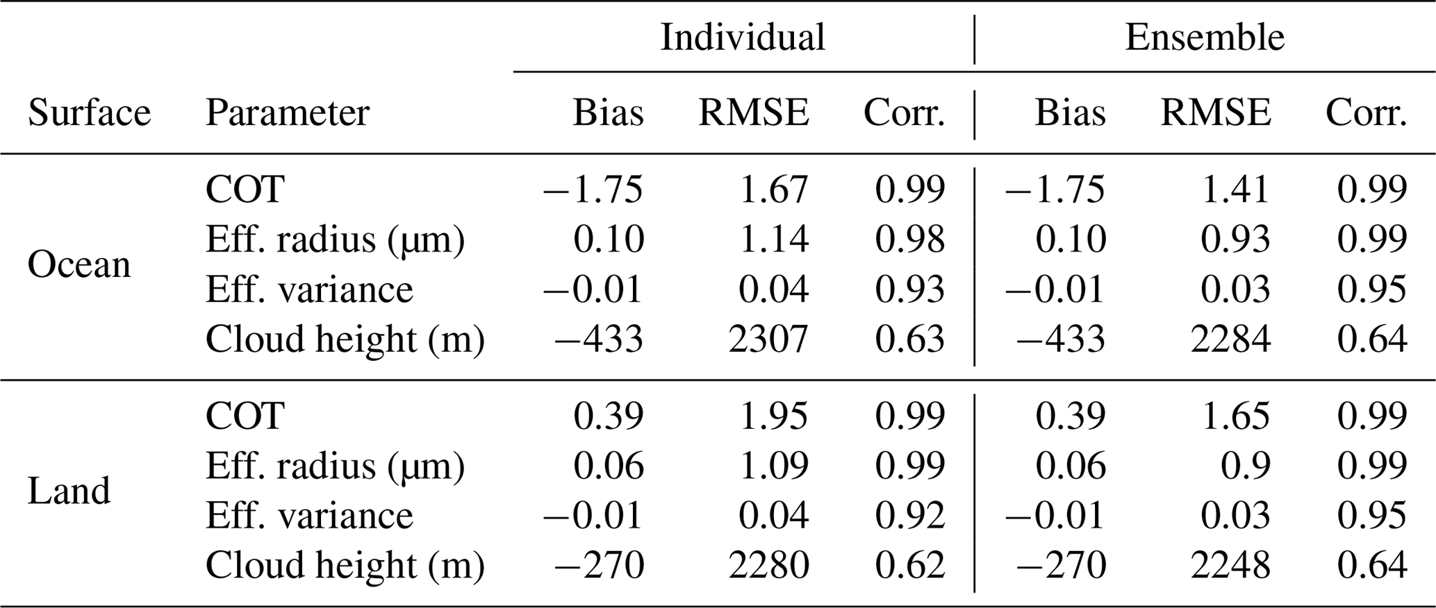
Figure 2Global distribution of snow cover and sea ice on 24 February 2006. Snow covered areas are shown in light pink, and sea ice areas are shown in dark pink. Data are from the MODIS-Aqua Normalized Difference Snow Index (NDSI) and sea ice products. Image is from NASA Worldview (https://worldview.earthdata.nasa.gov, last access: 11 March 2019).

While the results reported in Table 3 serve as an internal consistency check for the neural network performance, they cannot be used to predict the performance of our neural networks when applied to real measurements. In fact, our simulation set-up entails a number of simplifications which are typically not satisfied in real scenarios. Some of the most important simplifications are the following:

• Training and test data have both been generated using a one-dimensional radiative transfer model. Therefore, a degradation of the retrieval accuracy can be expected when three-dimensional effects are significant.

• The impact of an incorrect assumption about the cloud particle size distribution cannot be assessed, as all the data are generated with an assumed Gamma size distribution.

• The vertical distribution of cloud effective radius and effective variance is assumed constant. This is often not the case in reality (Martins et al., 2011; Zhang and Platnick, 2011; Zhang et al., 2012).

All the aforementioned assumptions may lead to biases in the retrieved cloud properties (Zhang and Platnick, 2011; Zhang et al., 2012; Miller et al., 2018). The assessment of the performance of our neural network scheme when applied to real measurements is be the object of the next section.

4.1 Comparison to MODIS Level 2 data: selected examples

In order to evaluate the performances of our neural network retrieval, we have compared our retrievals to the MODIS Level 2 product remapped on the POLDER-3 official sinusoidal grid (Zeng et al., 2011), made available from Centre National d'Études Spatiales (CNES) and Lille University's ICARE data archive (https://www.icare.univ-lille1.fr/archive/?dir=PARASOL/PM-L2/, last access: 11 March 2019). In this section we present the results of a global comparison between our retrieval and the MODIS Level 2 product on 24 February 2006 as an example. This date is particularly interesting because it contains a wide variety of situations, including cases that may prove challenging for our retrieval of cloud properties. A ZIP file containing daily global plots for the entire year 2006 is provided at the following FTP address: ftp://ftp.sron.nl/open-access-data/antonion/10.5194-amt-2018-345/Supplement (last access: 15 March 2019).

As shown in Fig. 2, snow-covered areas were present in several regions in the Northern Hemisphere, such as Central Asia, northeastern Europe, Scandinavia and North America. Furthermore, a significant dust outbreak took place over the Eastern Mediterranean Sea, as shown in Fig. 3.

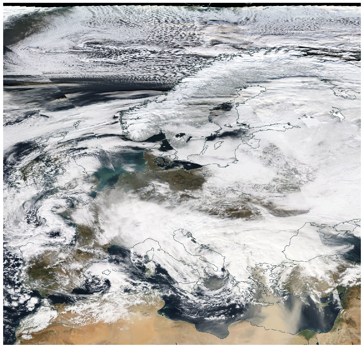
Figure 3A mosaic of MODIS-Aqua images showing Europe on 24 February 2006. Image from NASA Worldview (https://worldview.earthdata.nasa.gov, last access: 11 March 2019).

In Fig. 4, a global map of the COT retrieved by the neural network algorithm for POLDER-3 is shown together with an analogous maps produced by regridding the MODIS Level 2 product on the POLDER-3 resolution. The neural network product covers a narrower swath with respect to the MODIS product, as only pixels observed at a minimum of 14 viewing angles are considered in the NN retrieval.

In general, the spatial patterns of COTs seem to be well captured by the NN retrieval, but a number other aspects can be noticed in the maps. A first important remark is that at this stage we have not yet developed a cloud detection algorithm for our neural network product. As a consequence, the neural network will process all the available ground pixels regardless of whether they are actually covered by clouds. Nevertheless, it is interesting to see that over areas such as the Sahara – where a large number of cloud-free pixels are present – the NN correctly reports COTs very close to zero. As explained in Sect. 3.1, the NN has been trained on a variety of synthetic scenes, including situations of small COTs on bright, desert-like surfaces. However, the NN has not been trained on snow-covered synthetic scenes, and in such situations our neural network scheme seems to detect large COTs. This is clearly visible in Fig. 4, where an extended area of large retrieved COT can be seen over Central Asia. This area corresponds to the snow-covered region shown in Fig. 2. Similar features can be observed over North America. In general, distinguishing snow from clouds using POLDER-3 channels is extremely challenging if the observation geometry does not sample the cloudbow region (Bréon and Colzy, 1999). However, incorporating snow-covered scenes in the training set would be an interesting subject for future research in view of the application of our method to 3MI. In fact, 3MI will provide measurements at 1.6 µm, where snow has high absorption and can therefore be distinguished from clouds (Warren, 1982; Krijger et al., 2005, 2011) . An analogous behaviour of the NN COT retrievals can be observed over cloud-free regions covered by sea ice, such as the Hudson Bay, which appears to be covered by sea ice in Fig. 2 and exhibits large retrieved COTs in Fig. 4.

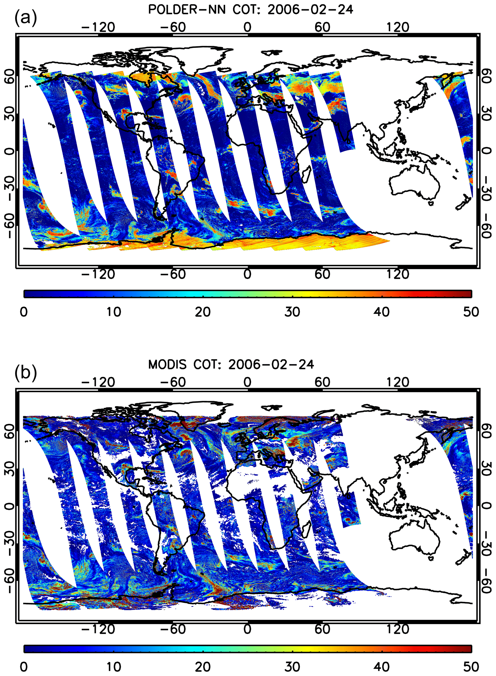
Figure 4Global cloud optical thickness maps on 24 February 2006 produced by the POLDER-3 neural network (a) and by MODIS (b).

Download

Other areas in which the NN retrievals differ significantly from MODIS data need a more careful inspection. Figure 5 shows retrieved COT maps over Europe for the NN algorithm and for MODIS. Both MODIS and the POLDER-3 NN generally see large COTs over the Balkans and in an area approximately centred around the Russian enclave of Kaliningrad. However, additional areas of large COTs can be seen in the NN map and not in the MODIS map. One approximately covers northeastern Italy, and a smaller one is centred on northwestern Spain, down the Bay of Biscay. A plausible explanation for this behaviour can be obtained by looking at the cloud phase index (CPI) product, described in Riedi et al. (2010), which can be used to estimate the cloud thermodynamic phase from combined POLDER-3 and MODIS data. Values of the CPI lower than 50 indicate liquid water clouds and values larger than 150 indicate ice clouds, whereas intermediate values indicate mixed-phase clouds. A map of the CPI over Europe for the selected date is shown in Fig. 6. The regions in which the NN retrieves much larger COTs than MODIS generally coincide with regions marked as ice clouds in the CPI map (CPI systematically larger than 170). These are not represented in the NN training set, and therefore the quality of the NN retrieval cannot be guaranteed over this type of clouds.

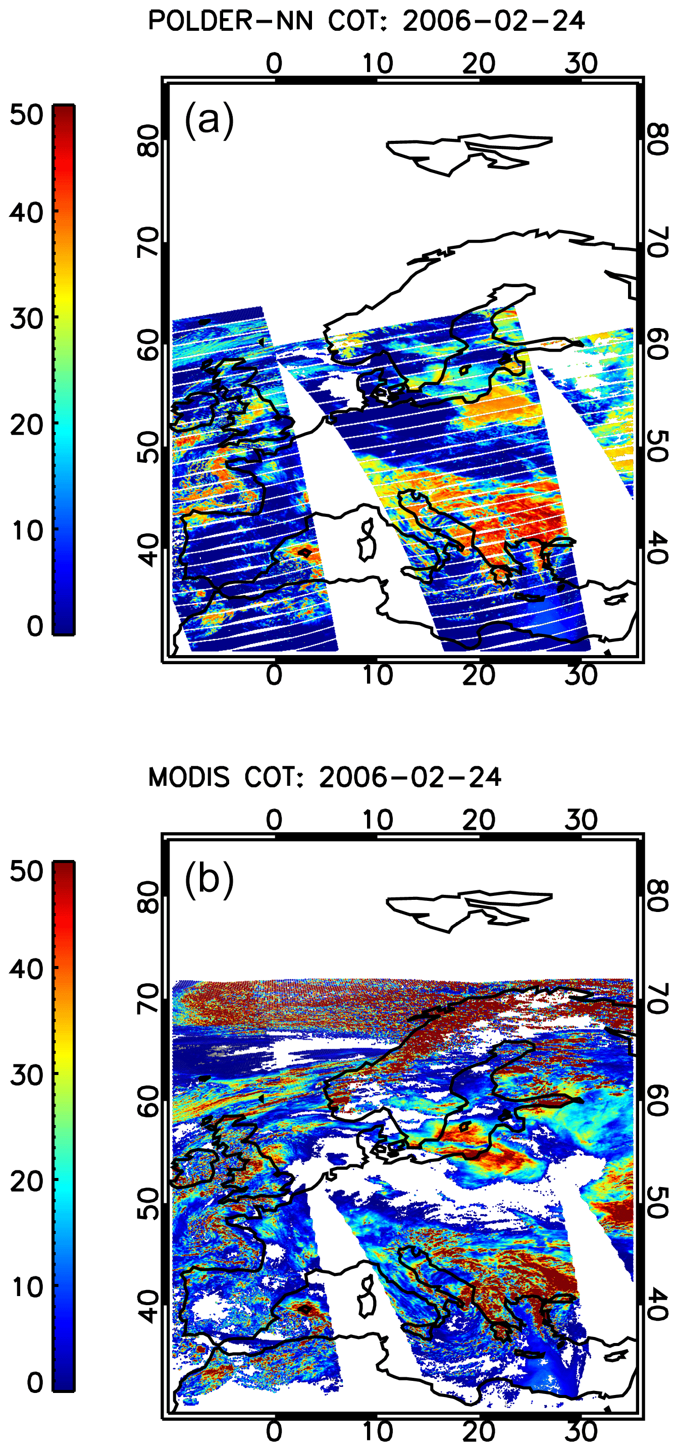
Figure 5Cloud optical thickness maps over Europe on 24 February 2006 produced by the POLDER-3 neural network algorithm (a) and by MODIS (b).

Download

In order to explain the origin of the bias in the retrieved COT over ice clouds, we can reason as follows. The reflectance of a cloud layer at nonabsorbing wavelengths can be approximated as follows (van Diedenhoven et al., 2014a):

where μ₀ is the cosine of the solar zenith angle, τ is the total optical thickness and g is the asymmetry parameter of the scattering phase function. If we take Eq. (2) as the reflectance of an ice cloud layer of optical thickness τ_ice, with asymmetry parameter g_ice, and assume the asymmetry parameter g_liq of a liquid water cloud in our retrieval, a liquid water cloud of optical thickness τ_liq with the same reflectance as that of the true ice cloud satisfies the relationship

Therefore, we can expect the estimated liquid water cloud optical thickness to be related to the true ice cloud optical thickness as approximately

Given that in the MODIS Collection 6 algorithm an ice cloud optical model with an asymmetry parameter of 0.75 is assumed (Holz et al., 2016), and that liquid water cloud droplets typically have an asymmetry parameter of around 0.85, based on Eq. (4) it is expected that our retrievals over ice clouds are biased by a factor of around 1.66 (van Diedenhoven et al., 2014b).

Histograms of the ratio between the COT retrieved by the NN scheme and that retrieved by MODIS over liquid water clouds (CPI <50), ice clouds (CPI >150) and mixed-phase clouds (50≤ CPI ≤150) are shown in Fig. 7 for the selected date. It can be seen that the peak of the histogram for ice clouds does not lie too far from the value predicted based on our simple approximation. The histogram for liquid water clouds, instead, is much more peaked around a value of approximately 0.8.

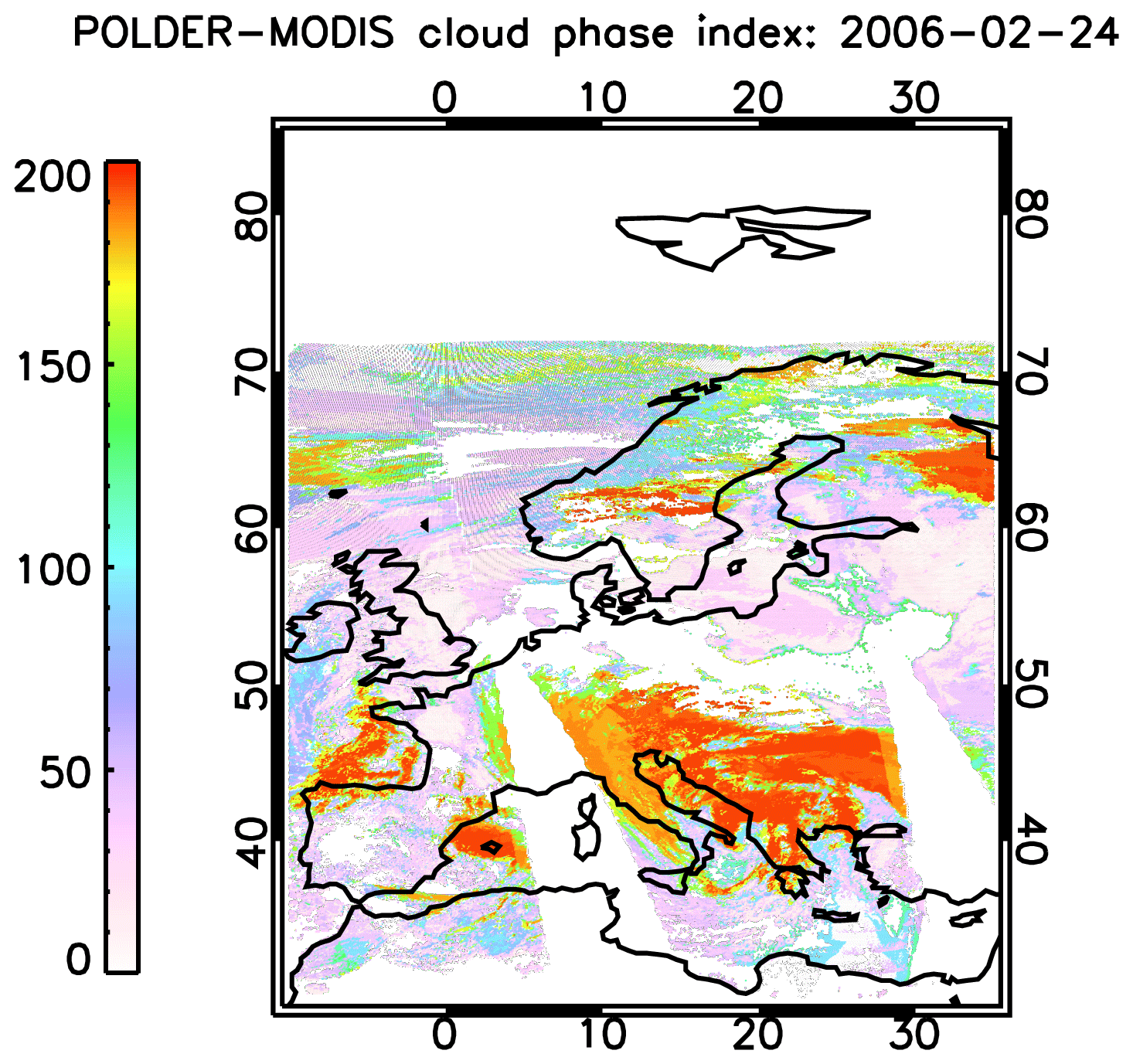
Figure 6POLDER–MODIS Cloud Phase Index over Europe on 24 February 2006. Data from ICARE – Laboratoire d'Optique Atmosphérique (LOA), University of Lille 1.

Download

Since our NN algorithm for COT retrieval does not just rely on single reflectance values but also uses the angular variability of reflectance and DoLP, it is expected that incorporating ice clouds in the training dataset may help to improve the COT retrieval accuracy over this type of clouds, at least reducing the spread of the histogram in Fig. 7.

In order to carry out a global quantitative comparison between the COTs retrieved by the neural network and those retrieved by MODIS over liquid water clouds, the following filtering criteria have been applied:

• The MODIS cloud fraction had to be larger than 0.95.

• The CPI had to be smaller than 50.

• Ocean regions affected by sun glint were not considered.

A pixel was flagged as affected by glint if observed from at least one viewing direction satisfying the following conditions:

• The relative azimuth angle was between −90 and 90^∘.

• The absolute difference between viewing zenith angle and solar zenith angle was smaller than 10^∘.

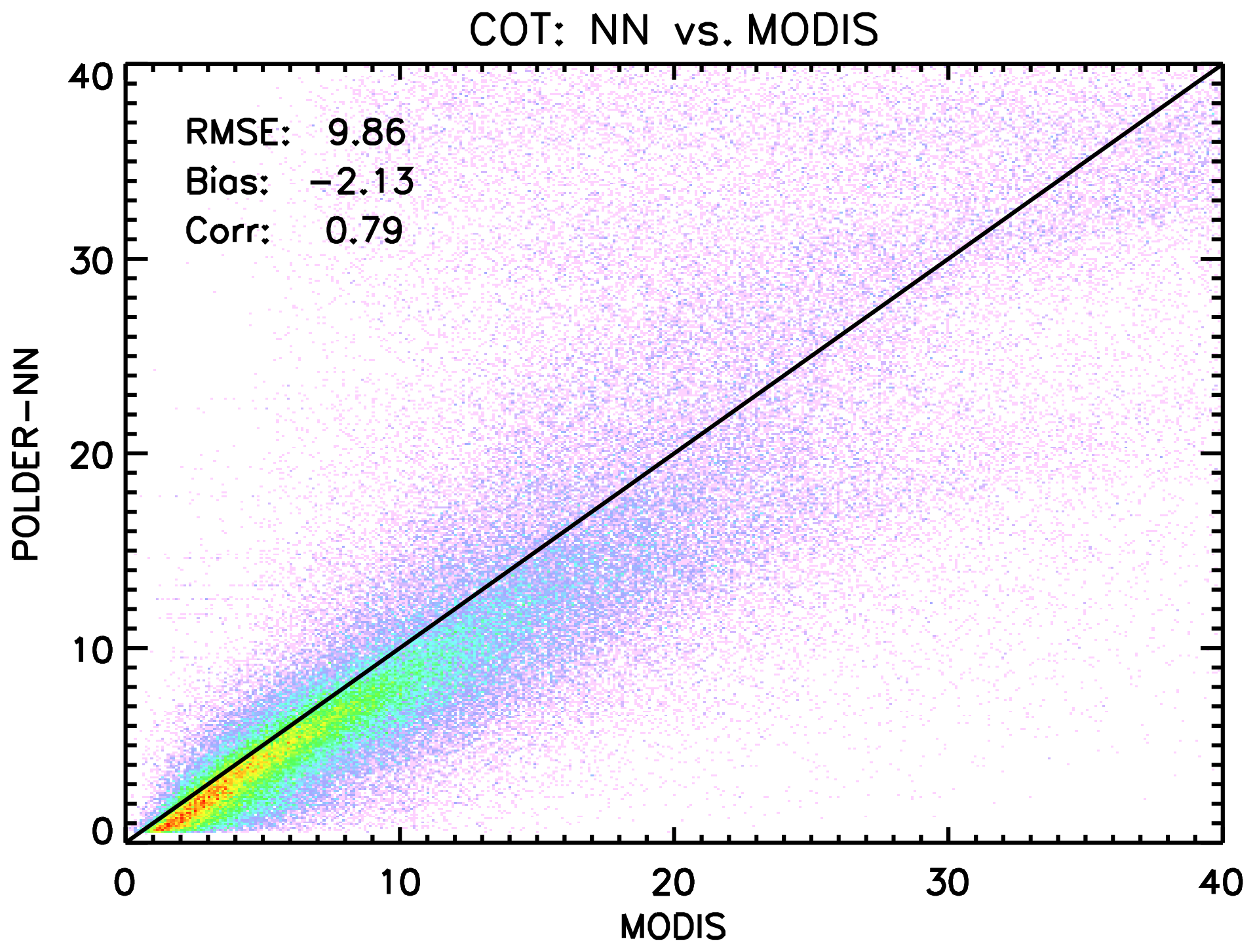
The results of the comparison are shown in Fig. 8, where it can be seen that the POLDER-3 neural network algorithm tends to retrieve systematically lower COTs with respect to MODIS, with a bias of around −2. Overall, the two datasets look fairly well correlated, with a correlation coefficient of 0.79.

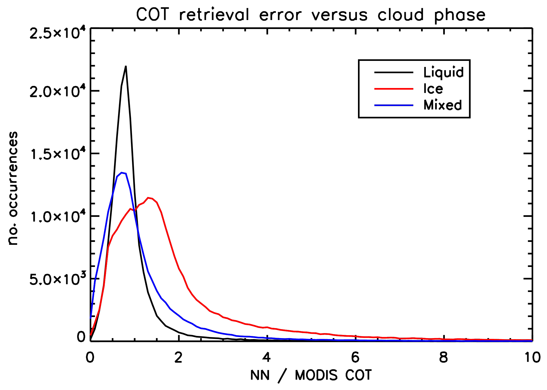
Figure 7Histogram of NN-to-MODIS COT ratios on 24 February 2006 over liquid water clouds (CPI <50), ice clouds (CPI >150) and mixed-phase clouds (50≤ CPI ≤150).

Download

Figure 8Global plot of POLDER-3 neural network versus MODIS COT on 24 February 2006.

Download

A similar comparison between the NN retrieval and MODIS has been performed for the cloud effective radius. Since the information on the cloud effective radius in POLDER-3 measurements mostly resides in the polarized radiance in the cloudbow scattering angle range, only pixels containing observations within this range were used in the comparison. More precisely, a POLDER-3 pixel was considered eligible for effective radius retrieval if it was observed in a scattering angle range satisfying the following two conditions:

• The minimum scattering angle was not larger than 135^∘;

• The maximum scattering angle was not smaller than 165^∘.

Such conditions were applied on top of the criteria mentioned above for the comparison of the retrieved COTs. The results of the comparison are presented separately for ocean and land in Fig. 9. Over both surface types, a negative bias in POLDER retrieved effective radii with respect to MODIS effective radii using the 2.13 µm band is observed. The bias is around −2 µm over ocean and −1 µm over land. The correlation coefficients are worse than for the COT, which is to be expected given the differences in sensitivity to vertical and horizontal inhomogeneities between the polarimetric and bi-spectral methods (Miller et al., 2016, 2018). Nevertheless, it appears that the NN retrievals are still capable of capturing some of the global patterns in the spatial variability in the cloud effective radius.

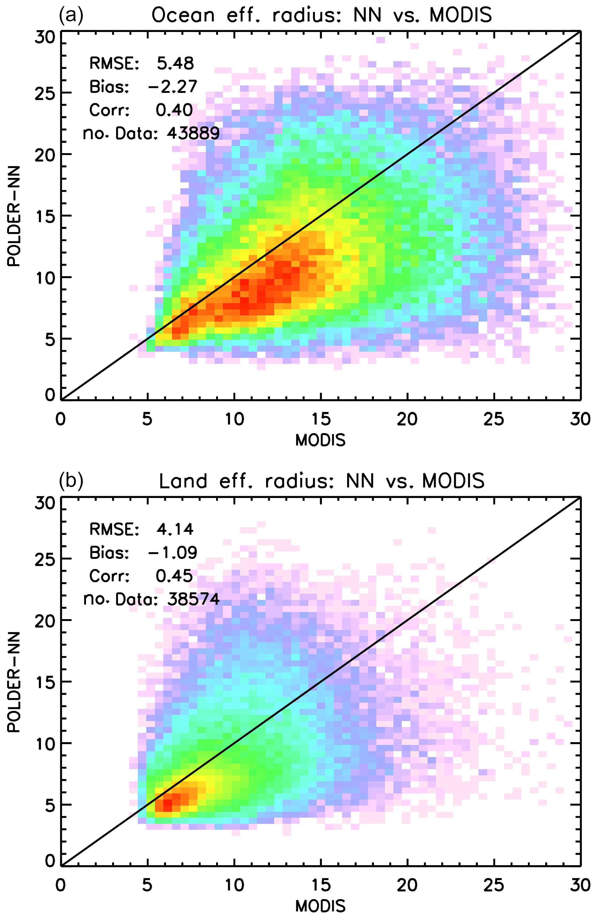
Figure 9Global plots of POLDER-3 neural network versus MODIS cloud effective radius (in µm) on 24 February 2006 over ocean (a) and land (b).

Download

Global histograms of the effective radii retrieved by the POLDER-3 NN over ocean and land are shown in Fig. 10. These seem to reflect the general knowledge of the fact that cloud droplets over land tend to be smaller than over ocean (Han et al., 1994; Bréon and Colzy, 2000; Bréon and Doutriaux-Boucher, 2005), thereby providing us with an additional sanity check for our retrievals.

4.2 Global comparison with MODIS Level 2 data

The comparison presented in Sect. 4.1, which refers to a particular day, highlights a number of features in the behaviour of our NN retrieval algorithm. We carried out a more systematic comparison by looking at the entire Level 2 dataset for the year 2006. In order to make the size of our datasets more manageable, we chose to rebin both the neural network retrievals and MODIS retrievals on a $\mathrm{1}{}^{\circ }\times \mathrm{1}{}^{\circ }$ grid. The data used in the regridding were filtered according to the same criteria explained earlier in this section for the example date 24 February. The fact that the same criteria were applied to both datasets, and the fact that the MODIS retrievals had already been remapped to the POLDER spatial resolution prior to the regridding, should minimize the risk of introducing greater biases at this processing stage.

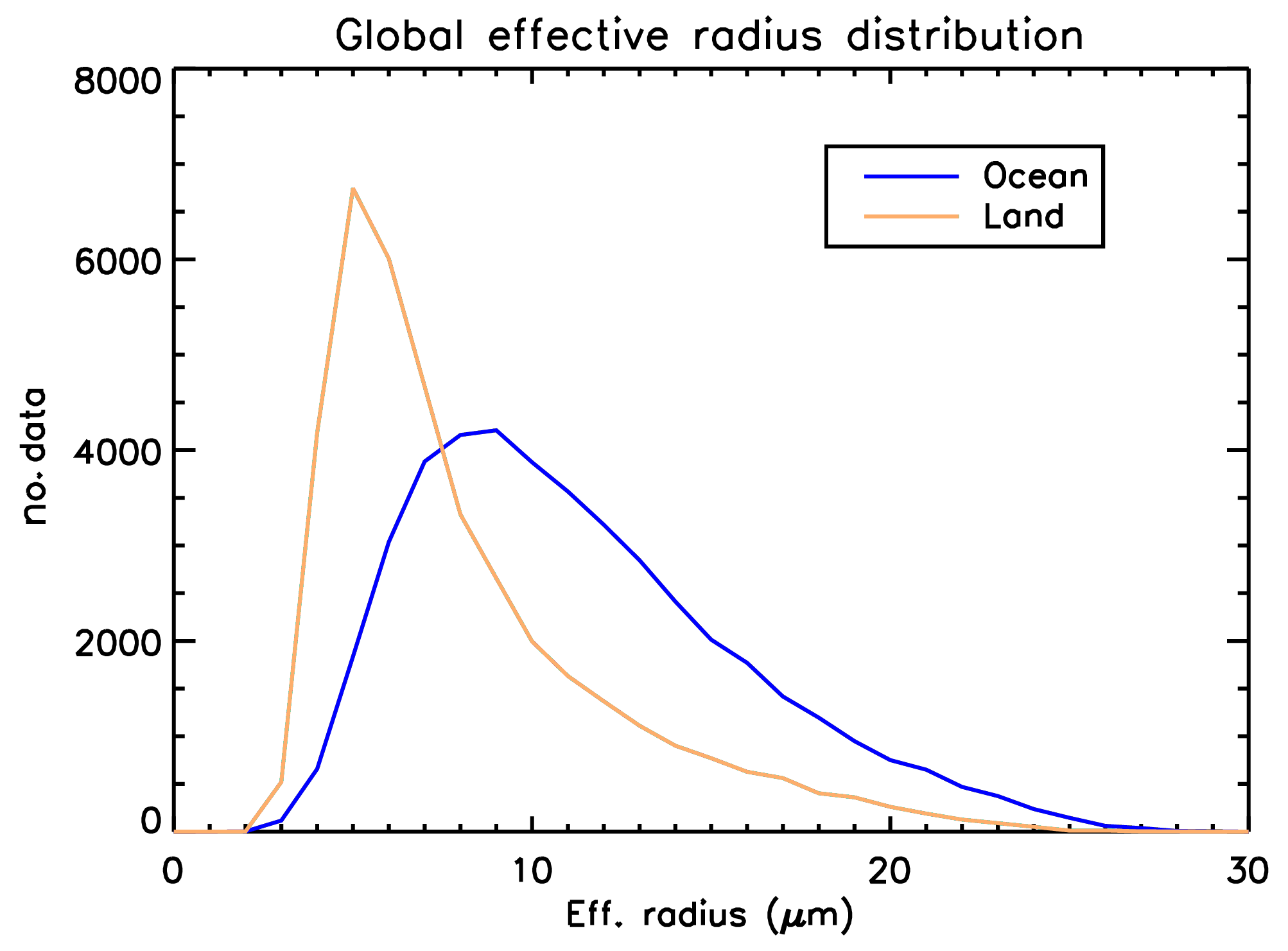
Figure 10Global histograms of cloud effective radii retrieved by the POLDER-3 neural network over ocean and land on 24 February 2006.

Download

The results of this global comparison for COT are shown separately for ocean and land scenes in Fig. 11. As for the effective radius, we observed a distinct behaviour in our retrievals between cases of “low clouds” (cloud top pressures larger than 600 hPa) and cases of “high clouds” (cloud top pressures lower than 600 hPa). As shown in Fig. 12, effective radius retrievals appear less biased with respect to MODIS, both over ocean and land over low clouds. It is important to note that both the POLDER-3 and the MODIS retrievals used in the rebinning were preliminarily filtered for ice using the POLDER–MODIS CPI, but it is still possible that cases exist in which the cloud phase identification is imperfect. This result suggested us to filter out clouds higher than 600 hPa in our global effective radius comparison. This filter has been used in all the comparisons that are shown hereinafter.

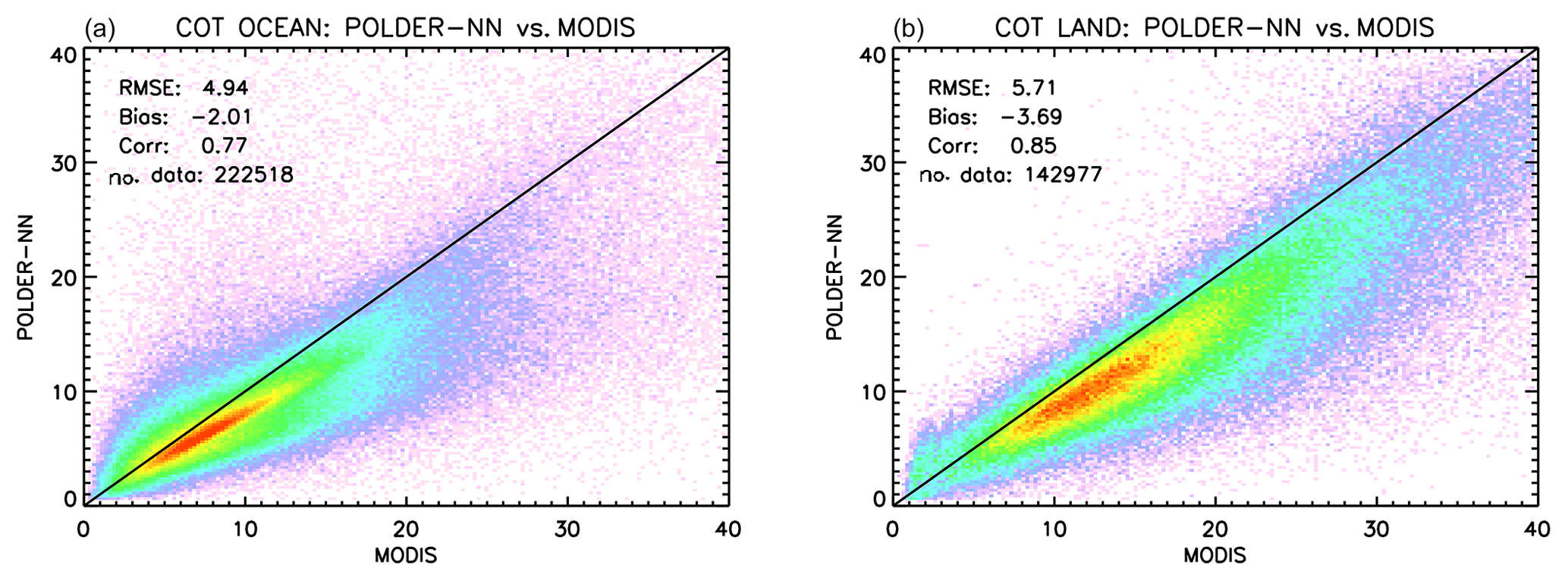
Figure 11Global comparison between neural-network-based POLDER-3 cloud optical thickness retrieval, and MODIS retrievals over ocean (a) and land (b) encompassing the full year 2006 on a $\mathrm{1}{}^{\circ }\times \mathrm{1}{}^{\circ }$ spatial grid.

Download

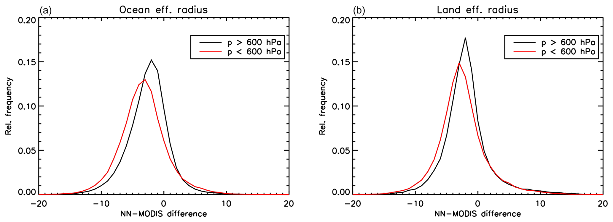
Figure 12Histograms of MODIS–NN effective radius retrieval differences (in µm) over ocean (a) and land (b), differentiated by cloud top pressure range.

Download

Scatter plots of the NN vs. MODIS effective radii over ocean and land are shown in Fig. 13. The NN-retrieved effective radii show a negative bias with respect to MODIS. Such bias appears fairly consistent between ocean and land. Looking at the scatter plot, there seems to be a “cluster” of points over land for which the NN retrieves much larger effective radii than MODIS. A preliminary investigation shows that these situations preferentially occur over southeastern China, around the Río de la Plata estuary in South America and along the southern part of the Bight of Biafra in Africa. This is shown in Fig. 14, which depicts a map of the data points over land where the MODIS retrieved effective radii smaller than 10 µm while the neural network retrieved effective radii larger than 18 µm. It is not clear, at this stage, if particular cloud types are associated with these areas or if that effect is caused by the presence of aerosols above clouds, which is at least possible over western central Africa (Waquet et al., 2009). Aerosols above clouds were not modelled in the training set of our neural network scheme and may have an impact on our retrievals when scattering angles between 100 and 120^∘ are present in the measurement vector, as Waquet et al. (2009) show that TOA polarized reflectances in this scattering angle range are significantly higher over a cloud with an aerosol layer above than they would be in absence of an aerosol layer. We have tried to identify cases of aerosol above clouds by means of an empirical filter on polarized reflectances between 100 and 120^∘, but so far we have found no conclusive indications regarding their impact on our cloud property retrievals. An additional element that can be noticed in the scatter plots in Fig. 13 (and in all the subsequent plots) is that the number of available data points over land is much smaller than over ocean. This is a result of filtering for high clouds, which reduced the ratio between the number of land and ocean data points from ∼55 % to roughly 39 %.

Figure 13Global comparison between neural-network-based POLDER-3 effective radius retrieval, and MODIS retrievals over ocean (a) and land (b), encompassing the full year 2006 on a $\mathrm{1}{}^{\circ }\times \mathrm{1}{}^{\circ }$ spatial grid. Effective radius values are in µm.

Download

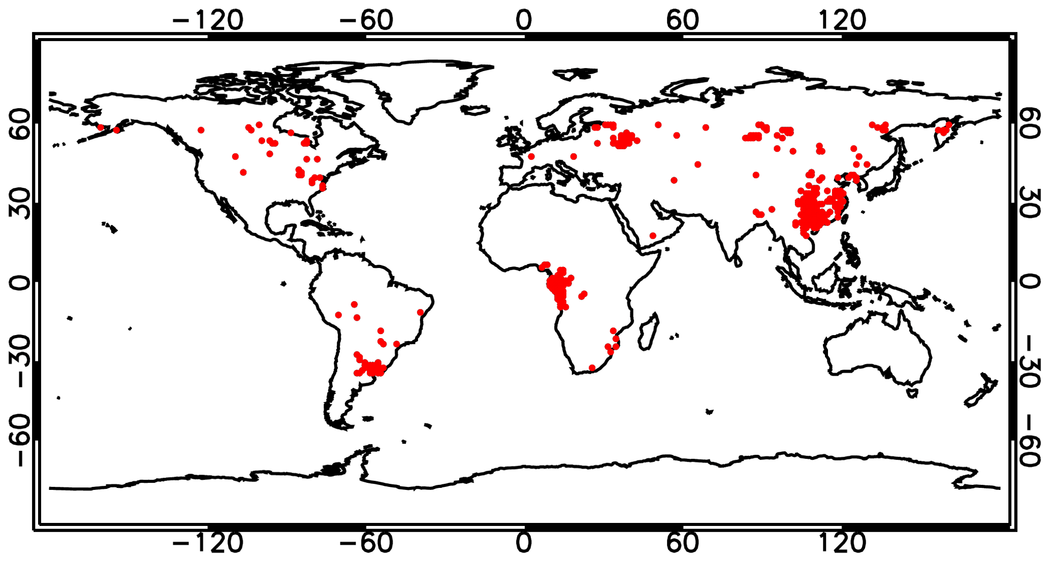
Figure 14Occurrence map of cases with MODIS effective radius smaller than 10 µm and NN effective radius larger than 18 µm, over land, during the year 2006.

Download

The bias observed in the retrieved effective radii seems consistent with results obtained with other algorithms (Bréon and Doutriaux-Boucher, 2005). The negative bias present in our COT retrievals is possibly explained by the presence of residual cases of broken clouds in our dataset, which are known to cause negative POLDER–MODIS differences (Zeng et al., 2012). On the contrary, the differences in the assumed cloud model should not be an important cause for the observed bias, as the uncertainty induced by changing the assumed cloud model in MODIS retrievals is estimated to be small (Platnick et al., 2017), with the exception of retrieval at special scattering angles such as cloudbow and glory (Cho et al., 2015). However, these situations only account for a very small fraction of MODIS retrievals.

4.3 Effective variance retrievals: preliminary results

As pointed out in Sect. 3.1, our NN scheme for cloud property retrievals does not assume a fixed effective variance but retrieves the effective variance together with the effective radius. This design choice is different from what is done in most of the existing cloud retrieval algorithms. In general, most cloud retrieval schemes assume a cloud model with a fixed effective variance ranging from 0.1 to 0.15, depending on the algorithm (Arduini et al., 2005, and references therein). In particular, a value of 0.1 is assumed in the MODIS Collection 6 products (Platnick et al., 2017). In the training set of our NN retrieval algorithms, effective variance was assumed to be uniformly distributed between 0.03 and 0.35. In the interpretation of the NN retrievals, this can be regarded as a sort of “prior distribution” for cloud effective variance. As shown in Table 3, our NN scheme seems capable of retrieving cloud effective variance to a good accuracy when applied to synthetic measurements. This impression is corroborated by the upper panel of Fig. 15, which is a scatter plot of retrieved versus true effective variances on a set of synthetic measurements over ocean. This test gives us some confidence in the possibility of retrieving effective variance from POLDER-3 measurements. In the lower panel of Fig. 15, a global histogram of effective variances retrieved by the NN over land and ocean on 24 February 2006 is shown. Histograms for other dates, which are available at the URL indicated in Sect. 4.1, are very similar to this one. On one hand, experiments on synthetic data seem to suggest that the NN should be able to retrieve effective variance within the typically assumed range of this parameter. On the other hand, when applied to real POLDER-3 measurements, the algorithm has a strong preference for effective variances around 0.05 over ocean and 0.06 over land, both smaller than the value assumed in the MODIS product. It is important to emphasize that, given the broad prior distribution used to train the NN, the behaviour of the NN when applied to real data appears to be entirely driven by the measurements. It is interesting to note that the result we observed over ocean has been recently found also by another study based on SEVIRI measurements over marine stratocumulus clouds, currently under review (Benas et al., 2019), using a method that is completely independent of the one presented in this article. However, it must be noted that the effective variances we retrieved over land are smaller than those suggested by other studies focussed on continental clouds (Miles et al., 2000; Khaiyer et al., 2005). Therefore, additional research will be needed on the interpretation of our effective variance retrievals.

Figure 15(a) Scatter plot of retrieved versus true cloud effective variance of synthetic data. (b) Global histograms of cloud effective variance retrieved by the POLDER-3 neural network over ocean and land on 24 February 2006.

Download

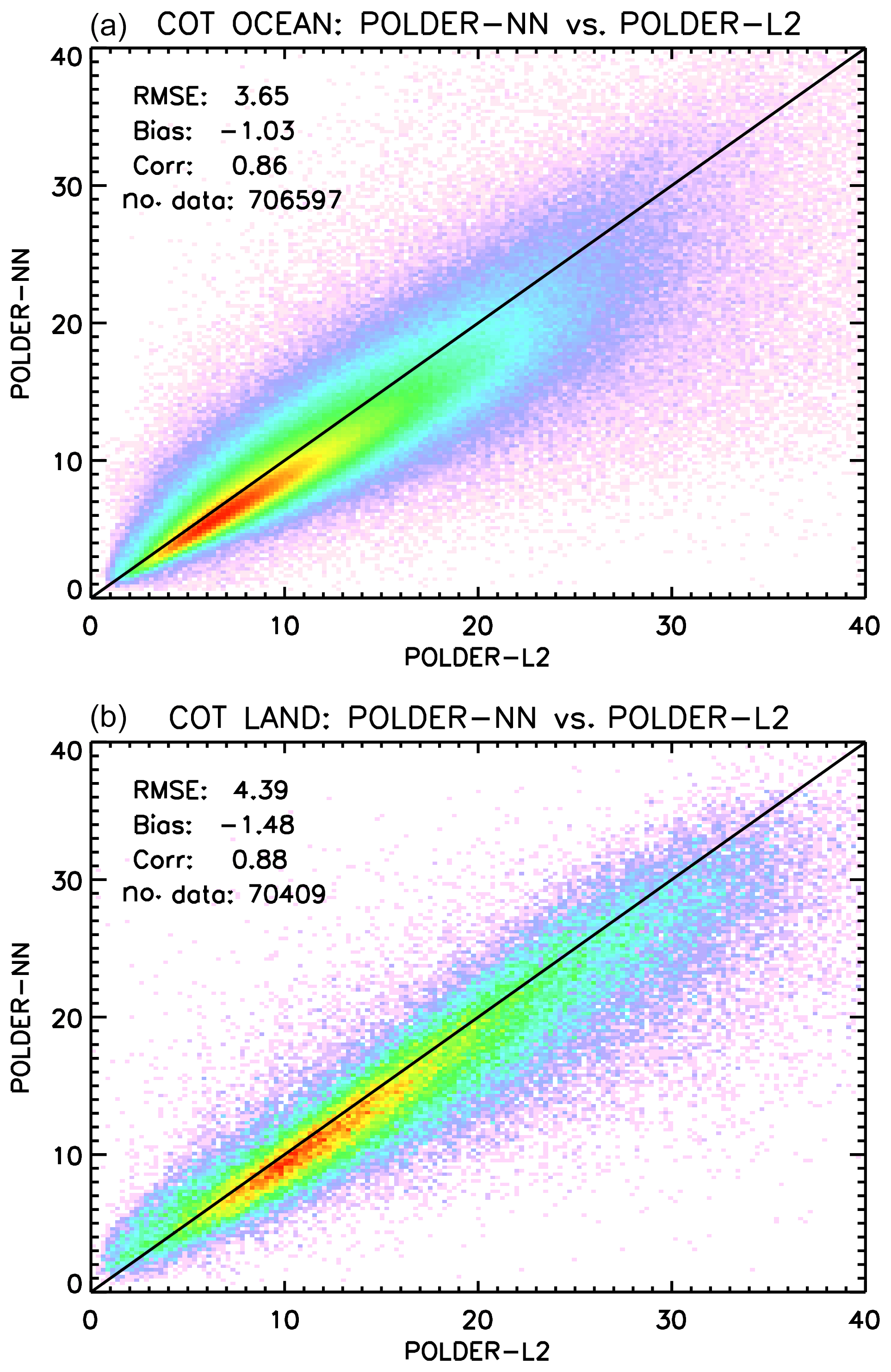
Figure 16Global comparison between POLDER-3 neural-network-based and Level 2 cloud optical thickness retrievals over ocean (a) and land (b) encompassing the full year 2006 on a $\mathrm{1}{}^{\circ }\times \mathrm{1}{}^{\circ }$ spatial grid.

Download

4.4 Comparison to existing POLDER-3 data and MODIS Level 3 data

In order to gain further insight on the behaviour of our retrieval algorithm, we carried out a global intercomparison between our retrieved COTs and effective radii to existing POLDER-3 retrievals. COT data at a spatial resolution of 20 km² ×20 km² are available from the existing POLDER-3 Level 2 product, whereas effective radius data are not included in the POLDER-3 Level 2 product, but are available from the Cloud Droplet Radius (CDR) product. Both products are available from the ICARE data archive mentioned in Sect. 4.1.

Also, for the comparison between the neural network retrievals and the existing POLDER-3 products, we have chosen a regular $\mathrm{1}{}^{\circ }\times \mathrm{1}{}^{\circ }$ grid. In order to better understand the difference between our retrievals and existing POLDER-3 products, we compared retrievals from both products to the MODIS MYD08_D3 daily product (Platnick et al., 2015). This also allowed us to compare effective radius retrievals to MODIS retrievals using the 3.7 µm channel, which are not available in the combined POLDER–MODIS Level 2 product. These retrievals are known to be more sensitive to the upper cloud layers compared to the standard MODIS product using the 2.13 µm channel (Platnick, 2000) and are therefore expected to be more comparable to polarimetric retrievals (Miller et al., 2016).

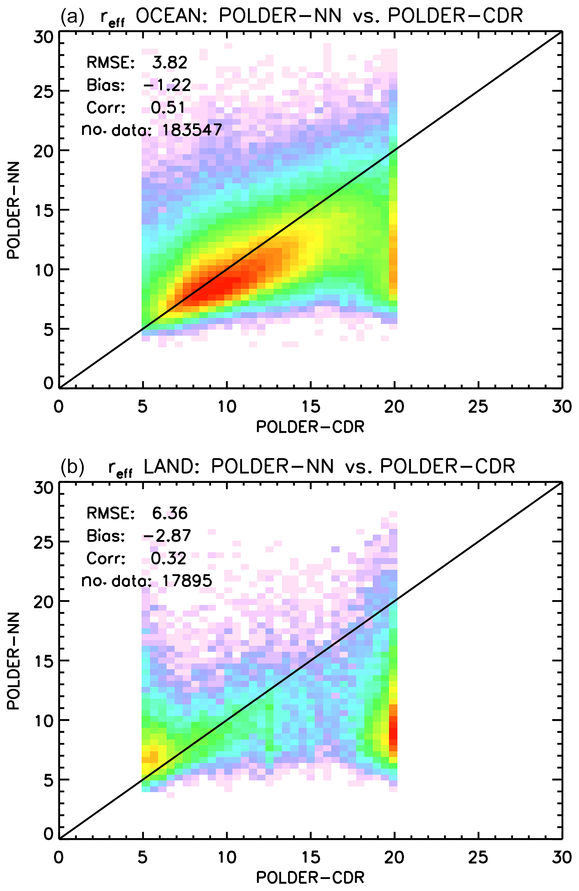
Figure 17Global comparison between POLDER-3 neural-network-based and CDR cloud effective radius retrievals over ocean (a) and land (b) encompassing the full year 2006 on a $\mathrm{1}{}^{\circ }\times \mathrm{1}{}^{\circ }$ spatial grid. Effective radius values are in µm.

Download

Figure 18Global comparison between POLDER-3 and MODIS 3.7 µm cloud effective radius retrievals over ocean, encompassing the full year 2006, on a $\mathrm{1}{}^{\circ }\times \mathrm{1}{}^{\circ }$ spatial grid. (a) Neural network. (b) CDR product. Effective radius values are in µm.

Download

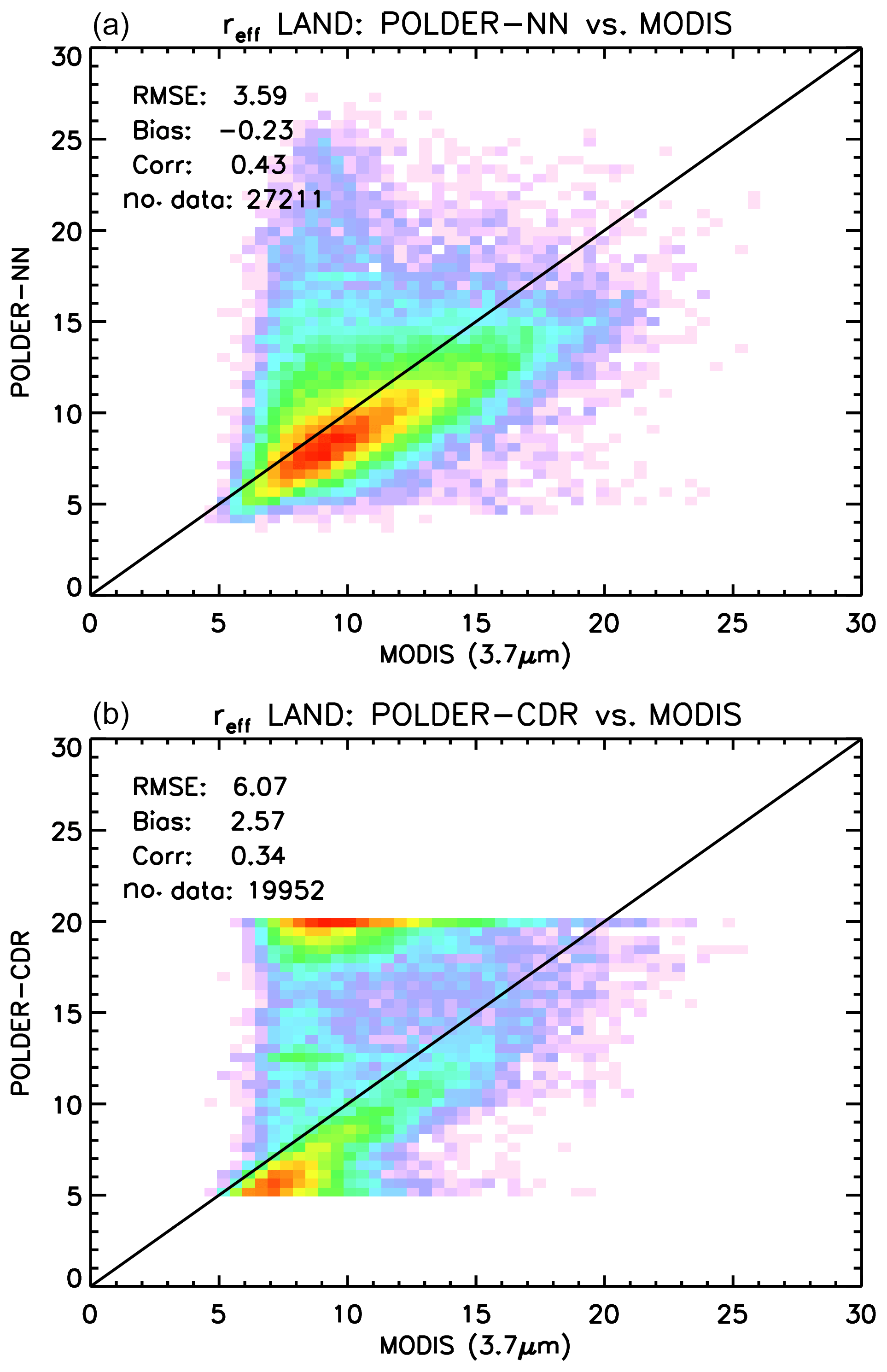
Figure 19Global comparison between POLDER-3 and MODIS 3.7 µm cloud effective radius retrievals over land, encompassing the full year 2006, on a $\mathrm{1}{}^{\circ }\times \mathrm{1}{}^{\circ }$ spatial grid. (a) Neural network. (b) CDR product. Effective radius values are in µm.

Download

The results of comparing neural network COT retrievals to POLDER-3 Level 2 retrievals are shown separately for ocean and land in Fig. 16. The correlation between the two retrieval schemes is high, although the NN retrievals are slightly lower than the Level 2 retrievals, with a low bias of around −1 over ocean and of around −1.5 over land. A possible reason for these systematic differences may lie in the different treatment of the cloud microphysical properties in the two algorithms. POLDER-3 Level 2 COT retrievals assume water droplets with a constant effective radius of 9 µm over land and 11 µm over ocean and an effective variance of 0.15 (Zeng et al., 2012), whereas in our retrieval these parameters are not fixed but are varied randomly in the training set.

A similar comparison is shown in Fig. 17 for cloud effective radius retrievals. In this case, the agreement between the neural network and existing POLDER-3 data is better over ocean than over land. A moderate negative bias of the neural network retrievals versus the CDR product exists over ocean, whereas over land the agreement is generally poor. We decided, then, to compare both datasets to gridded MODIS retrievals using the 3.7 µm channel. The results are shown in Fig. 18 for ocean and Fig. 19 for land. As expected, the negative bias of neural network retrievals versus MODIS 3.7 µm effective radii is smaller than that versus the 2.6 µm product. The existing CDR product seems more accurate and more precise than the neural network product over ocean, whereas the opposite seems to occur over land, where the neural network retrievals exhibit a significantly smaller bias versus MODIS compared to the CDR retrievals. Both over ocean and land, the bias of our neural network retrievals appears – in absolute value – smaller than 2 µm. An additional difference between our cloud effective radius retrievals and the CDR product is the fact that the latter seems to present a large number of cases in which the retrieved effective radius “saturates” to a value of 20 µm, whereas this does not seem to be the case for the NN retrieval. This difference probably results from the different choices made in generating the training set for the NN and the tabulated values for the CDR retrieval.