the Creative Commons Attribution 4.0 License.
the Creative Commons Attribution 4.0 License.
 | 19 Mar 2019
Adaptation and performance assessment of a quantum and interband cascade laser spectrometer for simultaneous airborne in situ observation of CH4, C2H6, CO2, CO and N2O
Julian Kostinek
Anke Roiger
Kenneth J. Davis
Colm Sweeney
Joshua P. DiGangi
Yonghoon Choi
Bianca Baier
Frank Hase
Jochen Groß
Maximilian Eckl
Theresa Klausner
André Butz
Tunable laser direct absorption spectroscopy is a widely used technique for the in situ sensing of atmospheric composition. Aircraft deployment poses a challenging operating environment for instruments measuring climatologically relevant gases in the Earth's atmosphere. Here, we demonstrate the successful adaption of a commercially available continuous wave quantum cascade laser (QCL) and interband cascade laser (ICL) based spectrometer for airborne in situ trace gas measurements with a local to regional focus. The instrument measures methane, ethane, carbon dioxide, carbon monoxide, nitrous oxide and water vapor simultaneously, with high 1 s–1σ precision (740 ppt, 205 ppt, 460 ppb, 2.2 ppb, 137 ppt and 16 ppm, respectively) and high frequency (2 Hz). We estimate a total 1 s–1σ uncertainty of 1.85 ppb, 1.6 ppb, 1.0 ppm, 7.0 ppb and 0.8 ppb in CH4, C2H6, CO2, CO and N2O, respectively. The instrument enables simultaneous and continuous observations for all targeted species. Frequent calibration allows for a measurement duty cycle ≥90 %. Custom retrieval software has been implemented and instrument performance is reported for a first field deployment during NASA's Atmospheric Carbon and Transport – America (ACT-America) campaign in fall 2017 over the eastern and central USA. This includes an inter-instrumental comparison with a calibrated cavity ring-down greenhouse gas analyzer (operated by NASA Langley Research Center, Hampton, USA) and periodic flask samples analyzed at the National Oceanic and Atmospheric Administration (NOAA). We demonstrate good agreement of the QCL- and ICL-based instrument to these concurrent observations within the combined measurement uncertainty after correcting for a constant bias. We find that precise knowledge of the δ13C of the working standards and the sampled air is needed to enhance CO2 compatibility when operating on the 2227.604 cm−1 13C16O2 absorption line.
- Article
(7506 KB) -
Supplement
(736 KB) - BibTeX
- EndNote


With steadily increasing greenhouse gas concentrations in the Earth's atmosphere, an improved understanding of the anthropogenic influence on climate is of major interest for global civilization. Globally averaged carbon dioxide (CO2) mole fractions have increased by 40 % since 1750. Methane (CH4) mole fractions have more than doubled since the preindustrial era, and over 60 % of this increase is estimated to be of anthropogenic nature (Ciais et al., 2013). Nitrous oxide (N2O) is a strong greenhouse gas and is expected to have the most important ozone-depleting anthropogenic impact throughout the 21st century (Ravishankara et al., 2009). Ethane (C2H6) is a powerful tracer commonly used to discriminate between different types of methane sources (Smith et al., 2015; Barkley et al., 2017; Peischl et al., 2015), and carbon monoxide (CO) is a marker for incomplete combustion processes and relates to the formation of tropospheric ozone (Klemm et al., 1996).
Aircraft provide a flexible platform for satisfying the fundamental need for accurate, temporally and spatially dense observations of these climatologically relevant gases from local to regional scales. Onboard meteorological data acquisition systems allow for concurrent observations of important atmospheric state variables like the local wind field, which is particularly useful to estimate emissions. Spectroscopic instruments making use of molecular ro-vibrational absorption allow for high temporal coverage through fast instrument response times (Chen et al., 2010). Some have already been used for airborne research, e.g., established IR spectrometers (O'Shea et al., 2013; Santoni et al., 2014; Cambaliza et al., 2015; Filges et al., 2015). Significant effort led to instruments operating in the mid-infrared (IR) region, e.g., liquid- nitrogen-cooled lead-salt diode laser-based spectrometers (Fried and Richter, 2007). With the commercial availability of continuous-wave lasers emitting in the mid-IR region near ambient temperature (Capasso, 2010; Vurgaftman et al., 2015; Kim et al., 2015; Beck et al., 2002) several new instrument designs have emerged (McManus et al., 2015; Zellweger et al., 2016). Quantum cascade laser (QCL) and interband cascade laser (ICL) based systems exploit several orders of magnitude stronger molecular absorption features in the mid-infrared compared to near-infrared-based instruments. Richter et al. (2015) reported on a custom-built difference frequency generation absorption spectrometer for simultaneous in situ detection of formaldehyde (CH2O) and C2H6 providing high detection sensitivities of 40 and 15 ppt, respectively. The custom-built airborne QCL spectrometer described by Catoire et al. (2017) allows for simultaneous observation of CO, CH4 and nitrogen dioxide (NO2) with in-flight precisions of 0.3, 5 and 0.3 ppb for a sampling time of 1.6 s. McManus et al. (2011) reported on the development of a high-sensitivity trace gas instrument based on quantum cascade lasers and astigmatic Herriott cells with up to 240 m path length. Unlike many established instruments measuring different species sequentially (one species after the other), the described spectrometer allows for concurrent sensing of the selected species and faster response times. These instruments have already been operated on different research aircraft. Santoni et al. (2014) describe the successful deployment and evaluation of a similar airborne spectrometer (Harvard QCLS) for more than 500 flight hours. However, Pitt et al. (2016) reported a severe cabin pressure dependency of their N2O and CH4 measurements using a commercial instrument (Aerodyne QCLS). By implementing a pressure-differentiated calibration method they were able to correct the corresponding dataset but had to omit roughly half of the measured data. Recently, Gvakharia et al. (2018) reported on a similar cabin pressure dependency for their N2O, CO2 and CO measurements (based on an Aerodyne QCLS). They suggested a fast calibration procedure to overcome these dependencies while maintaining a ≥90 % duty cycle.
Here, we describe the setup and performance of our flight-proven (over 100 flight hours) airborne QCL and ICL system developed for simultaneous airborne measurements of CH4, C2H6, CO2, CO, N2O and H2O. The instrument is shown to provide multi-species airborne observations for assessing greenhouse gas fluxes with a local (e.g., single facilities) to regional focus (e.g., urban agglomerations). Simultaneous observations of CH4 and C2H6 facilitate to pinpoint sources of CH4 enhancements (Smith et al., 2015). At the same time, the instrument provides measurements of N2O, the third most important greenhouse gas. This makes the instrument an ideal tool for airborne quantification and source attribution of greenhouse gas emissions using, e.g., the aircraft-based mass balance approach. Section 2 summarizes the refinements over the commercial system for use on aircraft. We show that frequent two-point calibration can mitigate cabin pressure dependencies. Section 3 describes our custom-built retrieval software developed for tuning the retrieval process. Sections 4 and 5 report on instrument performance in the laboratory and in the field during NASA's ACT-America fall 2017 campaign, including an inter-instrumental comparison with a calibrated cavity ring-down instrument and periodically taken flask samples. Section 6 summarizes our findings and concludes the study.
The spectrometer system used here builds upon the Dual Laser Trace Gas Monitor, a commercial tunable IR laser direct absorption spectrometer (TILDAS) available from Aerodyne Research Inc. (Billerica, USA), acquired by the German Aerospace Center (Deutsches Zentrum für Luft- und Raumfahrt, DLR) in late 2016. The basic instrument has already been extensively described in McManus et al. (2011). We will therefore only briefly introduce the basic instrument setup followed by a description of the refinements required to operate the instrument on a research aircraft.
2.1 Basic instrument setup
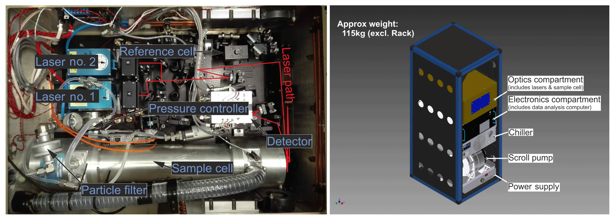
Figure 1Top-down photograph of the optics compartment (a). The sample cell made from aluminum along with the pressure controller and pressure transducers can be identified in the lower half. The QCL and ICL are mounted inside the blue housings to the left of the collimating Schwarzschild telescopes in the two black housings. The two detectors are mounted below the silver aluminum cases, housing the pre-amplifiers, on the right. The first detector is used for detecting both lasers after passing through the sample cell. The second detector is used for spectral referencing through an auxiliary optical path. Panel (b) illustrates the rack-mounted instrument. The figure includes solid models from Aerodyne Inc. and Solid State Cooling Systems.
The spectrometer is split into an electronics and an optics compartment. The electronics compartment includes an embedded computing system, thermoelectric cooling (TEC) controllers and power supply, etc. The optics compartment includes the lasers, the sample cell and the pressure controller, etc. Figure 1 shows a top-view photograph of the optics compartment. A combination of a continuous wave QCL and ICL measures mole fractions of CH4, C2H6, CO2, CO, N2O and H2O simultaneously using direct absorption spectroscopy. The sample cell is an astigmatic Herriott cell with approximate physical dimensions of () made from aluminum. It provides an effective absorption path length of 204 m with a net volume of 2.1 L. Two laser light sources are tuned to a specific center wavelength by adjusting the operating temperature using Peltier elements contained in the laser's housing. Excess heat is removed through a liquid cooling–heating circuit (Solid State Cooling Systems, New York, USA). Laser no. 1 is an interband cascade laser manufactured by Nanoplus GmbH, Gerbrunn, Germany, with a peak output power of 9.5 mW operated at 4.7 ∘C and modulated between 2988.520 and 2990.625 cm−1 using a linear current ramp of up to 40 mA. Laser no. 2 is a quantum cascade laser manufactured by Alpes Laser, St-Blaise, Switzerland, with a peak output power of 40 mW operated at 1.5 ∘C modulated between 2227.550 and 2228.000 cm−1 using a linear current ramp of up to 300 mA. The lasers are modulated sequentially at a fixed frequency of 1.5 kHz. Laser no. 1 scans over absorption lines of CH4, C2H6 and H2O, and Laser no. 2 sweeps over N2O, CO2 and CO lines. Each laser is sampled at 450 spectral points. Acquired spectra are co-added to yield a single output spectrum twice per second. Before reaching the sample cell, the laser beam travels approximately 1.6 m inside the instrument under ambient conditions. This will be referred to as the open path of the instrument, which is heavily influenced by variations in cabin pressure, temperature and humidity during airborne operation. After passing through the sample cell, the combined output from both lasers hits a single TEC detector. A second, identical detector collects radiation from two auxiliary paths. The first auxiliary path contains a small, sealed reference cell filled with CH4 and N2O. This allows for spectral referencing during system startup. The second path introduces an etalon into the beam, allowing for experimental determination of the laser tuning rate, which relates laser supply current and emitted wavelength.
2.2 Refinements for airborne operation
The key challenges for a successful deployment on research aircraft are limited space and power, the occurrence of linear and angular accelerations and large pressure, temperature and humidity fluctuations in both cabin and sampled air. Airborne instrumentation further requires a fast system response time, owing to the rapid movement of aircraft in the atmosphere. The response time is controlled by the time it takes to completely exchange the air in the sample cell which is driven by the highest achievable volumetric flow rate given a specific pump and sample cell volume.
Here, a scroll pump has been chosen to enable a constant sample flow through the sample cell. The lubricant-free scroll pump runs very smoothly, reducing vibrations of the measurement system, yet providing good pumping performance with a nominal value of 500 SLPM at standard conditions. This translates to a net flow rate of 25 SLPM (given IUPAC standard conditions of T=273.15 K and p=1000 hPa) when operating at a cell pressure of 50 hPa. Earlier experience showed that large electrical inrush currents have jeopardized nominal system startup (Stefan Müller, MPI Mainz, private communication, 2016). Sudden power failure, due to an overcurrent triggering aircraft circuit breakers, may lead to failures in the data analysis equipment. The original motor has therefore been exchanged with a synchronous three-phase motor (Baumueller Nuernberg GmbH, Velbert, Germany). This DC motor provides a rated power of 627 W at 28 VDC. By using a digital motor controller, the maximum startup current can be limited amongst various other tuning options. From previous studies the motor is known to emit a considerable amount of heat; a forced airflow provided by a standard axial fan ensures motor temperatures stay in the rated range.
Aircraft deployment requires the entire system to operate with a maximum of 50 A at 28 VDC. Power consumption of the instrument is mainly dominated by the pump and the thermoelectric cooling making up more than three-quarters of the total power requirement. Both components have been electrically converted without the need for power inverters from 230 VAC to 28 VDC to increase overall efficiency. The spectrometer and its internal computer are driven by a power inverter.
Large parts of the wiring harness have been exchanged from standard PVC cables to aviation-grade fire-resistant wiring. Mandatory electromagnetic compatibility and interference (EMC/EMI) tests have been carried out to comply with Federal Aviation Administration (FAA) regulations. The rack-mounted instrument sums up to a total mass of approximately 115 kg and has been tested to withstand linear accelerations of up to 9 g on the aircraft forward axis, 8 g on the downward axis, 6 g upwards and 2.25 g sidewards. Due to aircraft certification issues, pure water is used as process fluid for the liquid cooling–heating circuit instead of the intended propylene glycol∕water mixture.
A 3∕8 in. inner diameter hose made out of polytetrafluoroethylene (PTFE) has been chosen for the sample air intake as a compromise for pressure drop across the inlet and to minimize lag time between the inlet and the sample cell. Inside the instrument and upstream of the sample cell, an aerosol filter holds back particles bigger than 2 µm. The inlet is rear-facing, preventing large particle entrainment and protecting the instrument from liquid water and ice. Owing to the small diameter, the intake flow is inside the turbulent regime at all times (Re∼4000).
Finally, the sample cell pressure is regulated by means of a fully configurable pressure controller (Bronkhorst High-Tech B.V., Ruurlo, the Netherlands). A chip-scale temperature-compensated pressure transducer (Measurement Specialties, Ltd., Europe) and a humidity sensor (Sensirion AG, Staefa ZH, Switzerland) have been built into the optics compartment to allow the open-path state variables to be monitored (see Sect. 2.1).
2.3 In-flight calibration strategy
A custom-built calibration system has been implemented as illustrated in Fig. 2. Using mass flow controllers (MFCs; Bronkhorst High-Tech B.V., Ruurlo, the Netherlands), two gases can be mixed at arbitrary ratios.
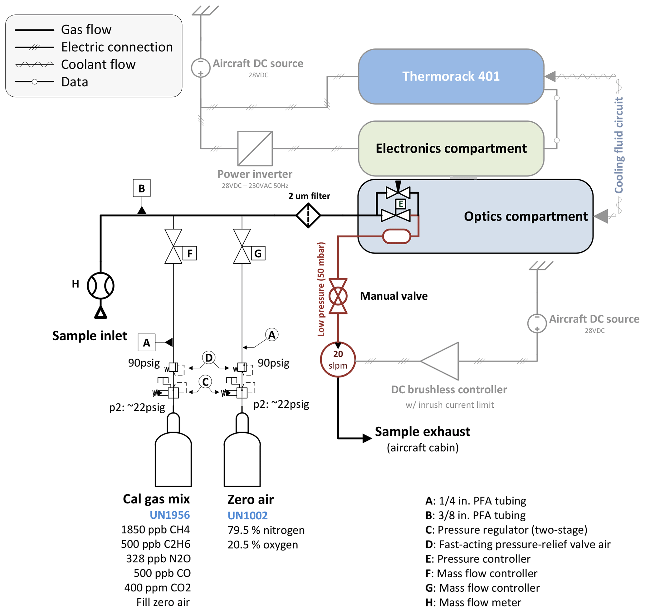
Figure 2Schematic showing the main components with emphasis on the calibration system. A mass flow meter allows the sample flow rate to be measured. Two reference gases can be mixed at any arbitrary ratio by means of two calibrated mass flow controllers. A 2 µm particle filter upstream of the sample cell avoids cell contamination.
The calibration gas mixture has been chosen to resemble “target” gas mole fractions close to atmospheric ambient values. The cylinders have been cross-calibrated against NOAA standards using a cavity ring-down spectrometer (CRDS) and are thus traceable to World Meteorological Organization (WMO) standards for CH4 (Cert.-Nr. CB11361, WMO X2004A for CH4 – Dlugokencky et al., 2005, WMO X2007 for CO2 – Zhao and Tans, 2006). C2H6, CO and N2O are compared to NOAA flask samples taken during the ACT-America field campaigns, which are also traceable to WMO standards. We use ultrapure synthetic air as “zero” gas instead of pure nitrogen (N2) to be in accordance with aircraft safety regulations and because the mole fraction of synthetic air (79.5 % N2 and 20.5 % O2) is chemically closer to sampled atmospheric air. Our calibration setup allows the net flow rate from the calibration cylinders to be slightly higher than the sample flow rate, minimizing pressure variations in the sample cell during switchover from normal to calibration sampling. To avoid contamination with cabin air, leak tests were carried out on a regular basis during the ACT-America field campaign. Histograms of typical calibration measurements are provided in Sect. S4 in the Supplement.
Owing to the high sensitivity of the retrieved mole fractions to changes in ambient conditions during flights (Gvakharia et al., 2018), calibration cycles are carried out automatically every 5 to 10 min. Each cycle consists of a pre-programmed sequence of flushing the sample cell with zero gas for 10 s followed by another 10 s of calibration gas. These time intervals have been found to be a good compromise between calibration gas cylinder endurance and measurement duty cycle. The online mixing feature is not used for in-flight calibration. Hence, no dilution of the calibration standard with zero air is introduced during flights, and the uncertainty in the flow rate measurements can be omitted. Online mixing (relevant for linearity checks) adds the uncertainty of the controlled mass flow (0.5 % relative error) on top of the gas cylinder uncertainties. Measured mole fractions of all detected species settle to an approximately constant value within the first 2 s after switchover from calibration gas to sample air and vice versa. The only exception is water vapor, which is observed to settle after approximately 30 s because of its stickiness and because the inlet tubing is made out of PTFE. The observed decay in H2O is different from the decay in other species in that a slow, almost linear decay follows the initial exponential decay, due to remaining water vapor in the inlet tubing and the sample cell.
The standard approach to retrieve dry-air mole fractions from the Aerodyne QCLS instruments is by making use of the software supplied by the manufacturer (TDLWintel). Here we utilize a custom retrieval software (JFIT) developed to double-check the output of the TDLWintel software and to enhance the ability of tweaking the retrieval process. Our main goal in developing a stand-alone algorithm here was to learn about possible error sources and mitigation possibilities of instrument dependencies and to be able to extend the instruments capabilities in the future.
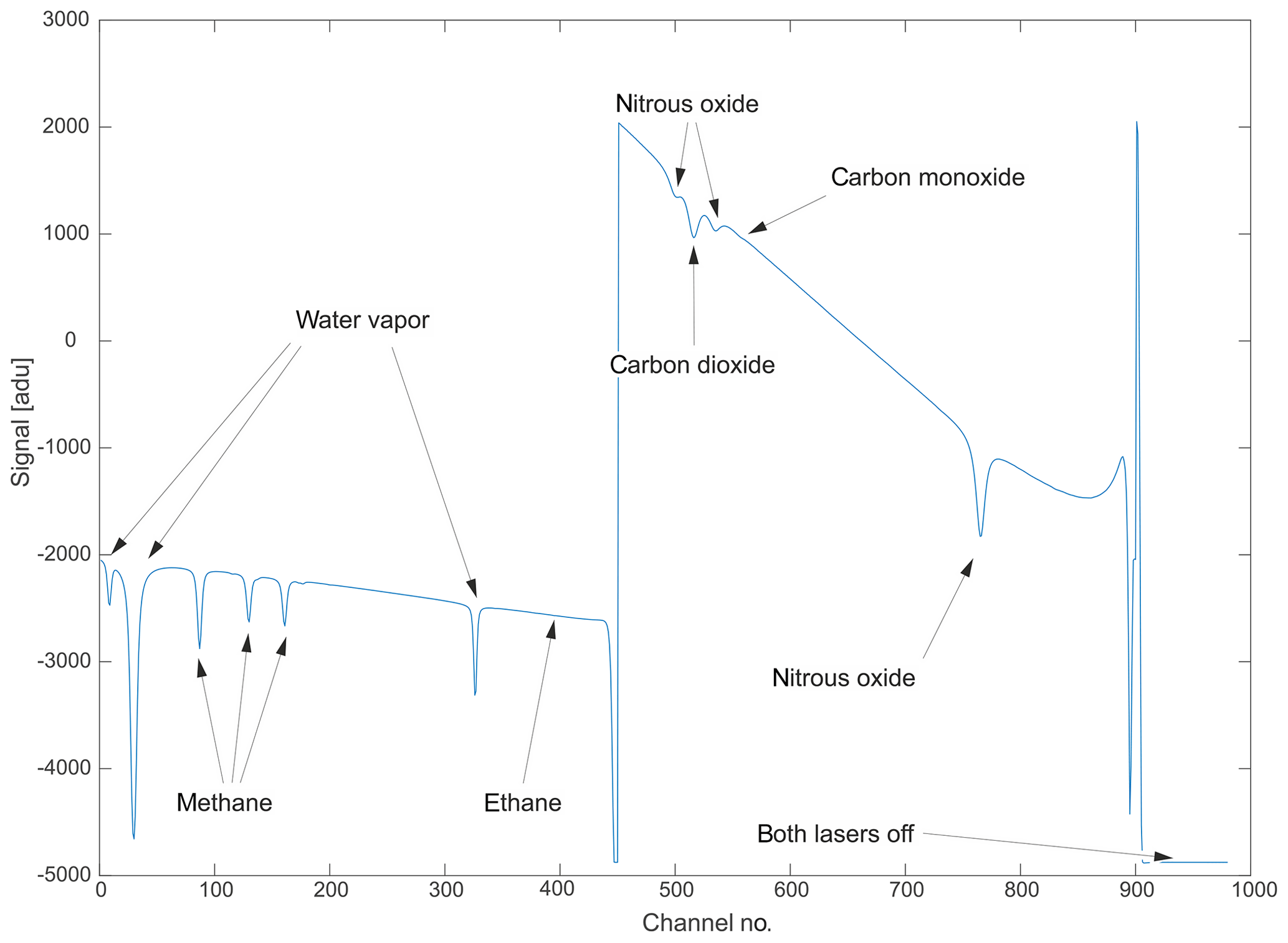
Figure 3A typical raw spectrum as recorded in binary format by the instrument. Arrows have been added to ease identification of the observed chemical species. Channel numbers on the abscissa can be converted to spectral units using the laser tuning rate. The intensity offset can be corrected by shifting the entire spectrum to yield zero intensity when lasers are turned off.
The code is written in plain C++. It digests the sample cell pressure and temperature measurements to generate a synthetic spectrum based on line-by-line parameters from the HITRAN2012 and HITRAN2016 (Rothman et al., 2013; Gordon et al., 2017) database using a conventional Voigt profile approach. Ethane line-by-line data have been taken from high-resolution Fourier-transform infrared spectra due to deficiencies in the HITRAN data for this particular species–wavenumber combination (Harrison et al., 2010). The computation of the Voigt profile has been adopted from Abrarov and Quine (2015). Our retrieval code differs from the TDLWintel approach in the determination of the spectral baseline and the handling of shift parameters and open-path water absorption.
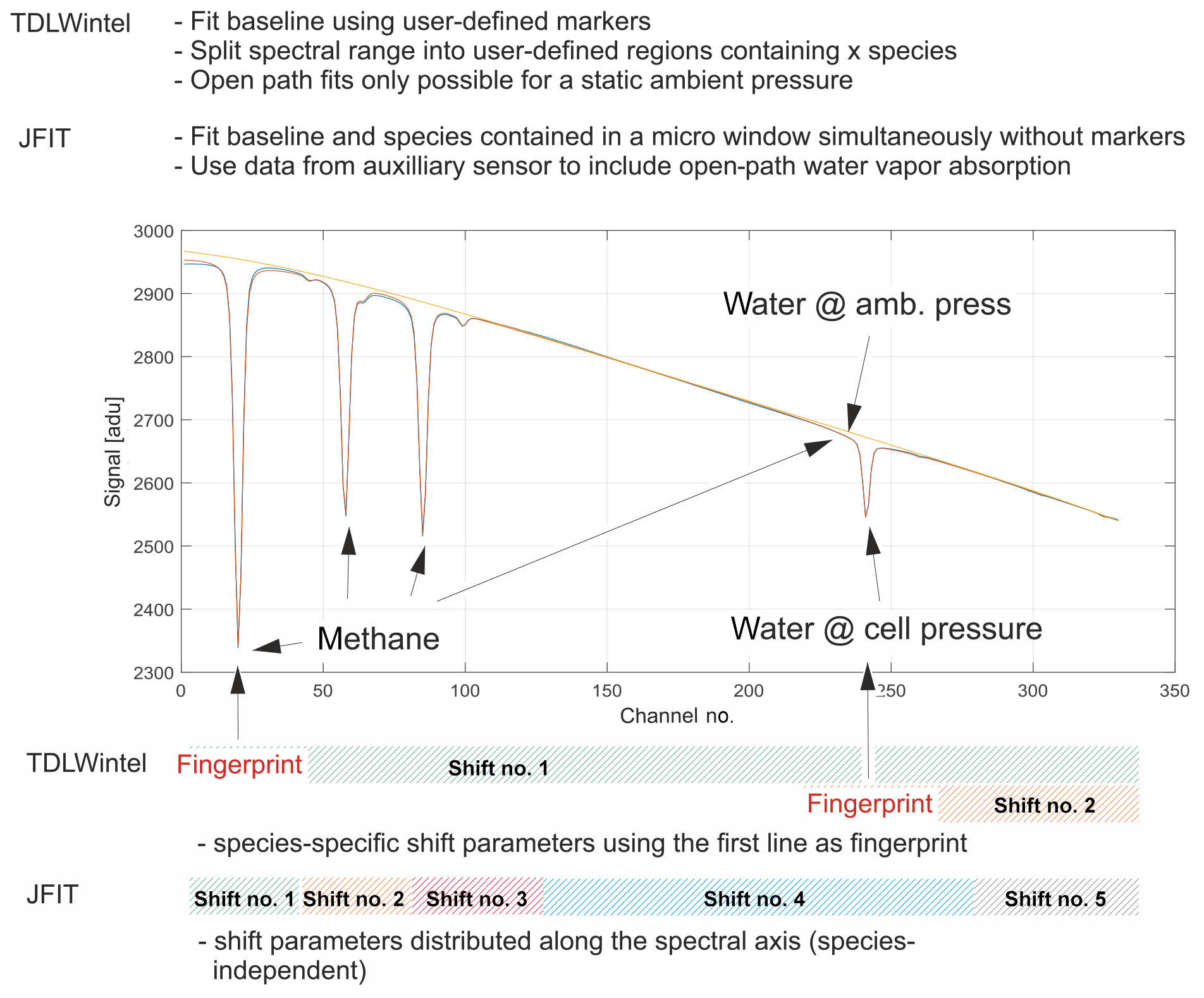
Figure 4Schematic depicting the handling of spectral shift parameters and baseline modeling. The spectral baseline is fitted as a polynomial together with absorption features over the entire fit window. Shift parameters have been implemented in a species-independent way. Open-path water is also included in the model.
A typical raw spectral output, as saved by the instrument in binary format, is illustrated in Fig. 3. The two consecutive laser scans are clearly visible. On the left side, Laser no. 1 sweeps between 2988.520 and 2990.625 cm−1 and, hence, over absorption features of CH4, C2H6 and H2O. The right side corresponds to the wavelength range of Laser no. 2 (2227.550 to 2228.000 cm−1) and includes absorption features of N2O, CO and CO2. After the lasers have scanned their full range, both lasers are completely turned off to allow for the determination of the detector zero-intensity offset. The abscissa corresponds to the individual sampling points, which can be converted to spectral units using the known laser tuning rate. The flat sections of the spectrum with no molecular absorption are considered to represent the spectral baseline. The shape of this baseline is mainly controlled by laser characteristics, the detector response function and optical properties of the installed mirrors and windows inside the instrument.
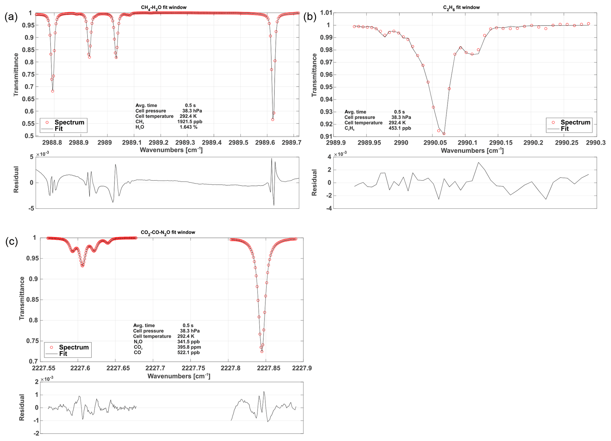
Figure 5Typical, normalized spectra for each fit window including fits and associated residuals. The first fit window (a) includes CH4 and H2O absorption features. Panel (b) depicts C2H6 absorption. The (c) spectrum shows CO, CO2 and N2O absorption.
The spectrum is broken down into three fit windows for the retrieval process (see Fig. 5). These were chosen based on the best overall performance found in retrieval tests and named after the chemical species included. A synthetic spectrum, including a polynomial representing the spectral baseline, is generated and fitted using an unbounded Levenberg–Marquardt least-squares algorithm (Marquardt, 1963). The degree of the background-fitting polynomial has been adjusted empirically for each different fit window. Species-independent shift parameters have been included, allowing individual absorption features to freely move on the spectral axis. Special care has been taken to group weak and strong absorption features together in a single shift parameter to provide sufficient certainty on their spectral positions. In other words, not every absorption line has its own shift parameter, but they are grouped as schematically shown in Fig. 4. As a result, only five shift parameters are included, although the synthetic spectrum in Fig. 4 is composed of more than 20 individual lines. When the absorptivity does not yield enough certainty to ensure proper determination of the shift parameters for a single spectrum, the shift variables are held constant at their means over the last 10 values. If another species in the relevant fit window allows for a proper determination of the spectral position, remaining shift parameters are coupled to those with enough certainty. This allows absorption line center frequency changes to be properly modeled and provides a means for observing spectral stability. Typical shift parameters for ground-based operation are given in Fig. 8 for the CH4–H2O and CO2–CO–N2O fit windows. Pressure, humidity and temperature data obtained from within the optics compartment are used to model H2O absorption at cabin pressure in the open-path region.
The CH4–H2O fit window covers almost the entire set of spectral features covered with Laser no. 1 except for the C2H6 absorption features. The spectral baseline is modeled as a third-order polynomial over the full range of the fit window. A typical spectrum including fit is depicted in Fig. 5 along with typical spectra for the other two fit windows.
The C2H6 fit window includes absorption features of CH4 and C2H6. The main challenge of retrieving precise C2H6 mole fractions arises from its very low background concentration in the atmosphere (approximately 1.05 ppb in the Northern Hemisphere; Simpson et al., 2012). A single adjacent CH4 line, located at 2989.981 cm−1, has been included in order to obtain C2H6 data, even under these challenging conditions. In this case, the weak CH4 absorption is not modeled as a free parameter and is hence not used for retrieving the CH4 mole fraction but for localizing the spectral position/shift parameter of the C2H6 absorption feature in the absence of a clear C2H6 signal. The CH4 mole fractions are fixed to the values determined from the previous fit window. Using this approach, we found a clear improvement in the C2H6 data quality including a higher precision and the absence of discontinuities. The associated spectral baseline is modeled as a second-order polynomial.
The CO2–CO–N2O fit window covers the entire second laser and is the most complex spectral scene. It includes several overlapping absorption features, making the retrieval of mole fractions of the targeted species challenging. As illustrated in Fig. 5, a single CO2 absorption line is surrounded by two N2O lines. The CO line is directly adjacent to one of the N2O lines. This results in comparatively large signal noise and increased uncertainty in the retrieved mole fractions due to crosstalk between the N2O, CO and CO2 absorption lines. However, the spectral range includes another N2O line at 2227.843 cm−1, which is slightly stronger than the other two (see Fig. 5). Our approach is to fix the mole fractions of the first two N2O lines to the stronger third one, in order to reduce the uncertainty in retrieved N2O and hence the noise on the CO2 and CO retrieval. The spectral baseline has been split into two parts, the first covering the first two N2O, CO2 and CO lines and the second covering the individual N2O line only. Both are modeled as second-order polynomials.
3.1 Water vapor correction
In the current instrument setup, water vapor is not removed from sampled air before entering the sample cell. Therefore, the influence of water vapor on the retrieved mole fractions has to be corrected in order to report dry-air mole fractions. Here, we correct for both dilution and water broadening effects. The first describes the fact that concentrations appear smaller when analyzing moist air, although the dry-air mole fraction might be constant. This effect can be remedied if the absolute water concentration is known for each individual sample using Eq. (1):
where cd is the dry-air mole fraction, cx is the raw concentration of a particular species of interest diluted in moist air and is the water vapor concentration (Harazono et al., 2015). Spectroscopic water broadening effects are approximately an order of magnitude smaller than dilution effects; yet they do have to be corrected for to obtain precise measurements. HITRAN's air broadening parameters are listed for a particular chemical composition of air excluding water vapor. H2O, however, can be a more potent broadening agent than nitrogen or oxygen (Kooijmans et al., 2016).
Table 1Empirically determined water vapor foreign broadening coefficients.

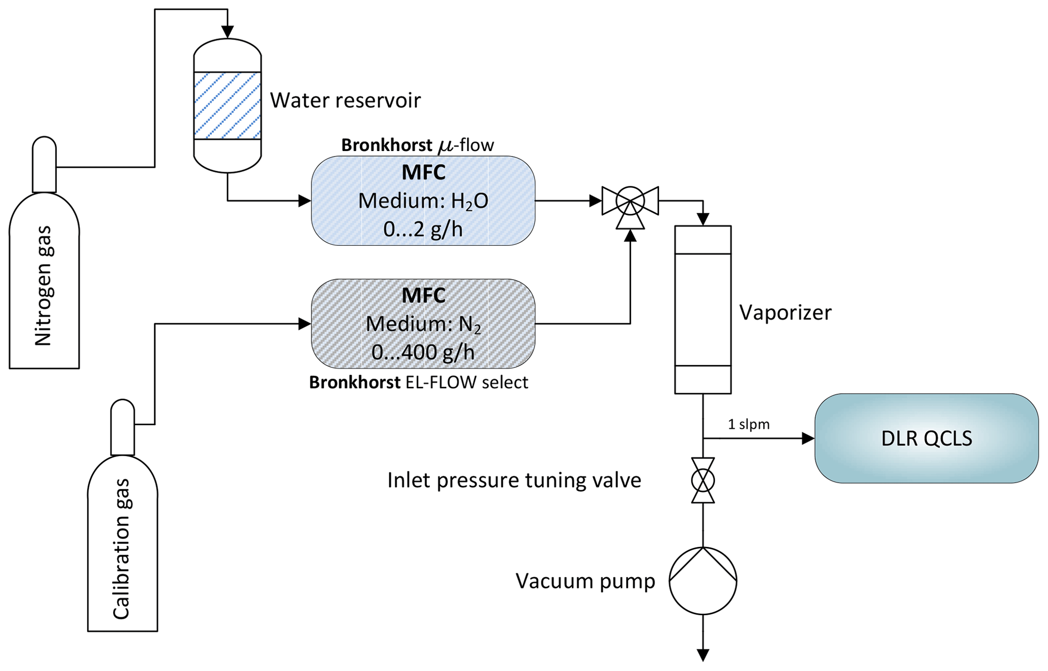
Figure 6Schematic depicting the water correction lab setup. A reference gas can be humidified to typical atmospheric values between 0 % and 2 % absolute water using mass flow controllers and an electronically controlled vaporizer. A downstream pump allows for simulation of different flight levels.
These coefficients have been determined using the setup depicted in Fig. 6 and are summarized in Table 1. Therefore, the pressure broadening has to be modified to include this effect. Under dry-air conditions it is common to split the pressure broadening into two parts: self-broadening and air-broadening. The self-broadening coefficient allows computation of the broadening induced by mutual collisions of a particular species of interest. The air-broadening coefficient can be used to approximate the broadening induced through collisions of a particular species with all the other species in a given air standard excluding the species itself. From the HITRAN definitions, the pressure-broadened half width at half maximum for a gas at pressure p and temperature T is given by
where Tref is a fixed reference temperature (Tref=296 K), pself is the partial pressure of a particular species of interest and nair is the coefficient of the temperature dependence of the air-broadened half width. This model has been extended to include collisions with H2O molecules yielding
with the partial pressure of water vapor and the water broadening coefficient . The former can be computed from the measured water vapor concentration. The latter can be empirically determined. Not including the self and water foreign broadening leads to relative errors in the range of 0 %–2 % for the described setup, depending on the species of interest. While small for C2H6 and CH4 with <0.03 %, the influence on retrieved CO is rather large with ∼2 %. In order to obtain , two MFCs are used to modify mole fractions of water vapor in a clean and dry calibration gas. This does not involve measuring water vapor at absolute levels; instead it is only necessary to span the range of atmospheric H2O. An additional downstream pump allows, in combination with a manually controlled needle valve, the absolute pressure at the instrument inlet to be tuned to simulate altitude changes. For these tests, the QCLS instrument has been operated at low flow rates of approximately 1 SLPM due to limitations on the two mass flow controllers. The water broadening coefficient has been adjusted iteratively until reported dry-air mixing ratios of the species of interest remained constant for the set of water vapor mole fractions.
Extensive ground-based instrument checks have been conducted, including tests in a pressure chamber at the Karlsruhe Institute of Technology (KIT) and laboratory tests at DLR Oberpfaffenhofen, Germany.
Table 2Typical 1 s–1σ precision during ground-based instrument checks.
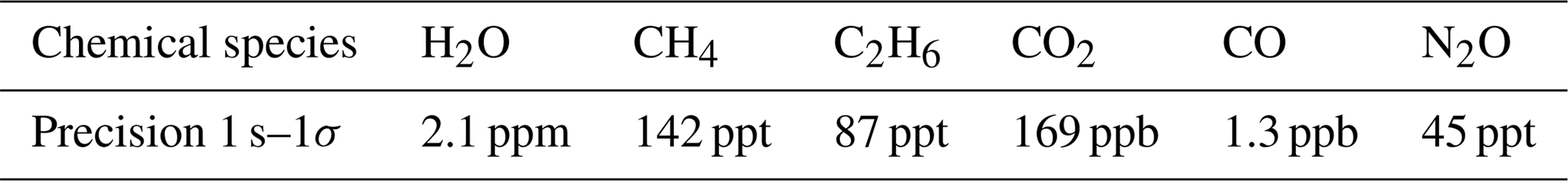
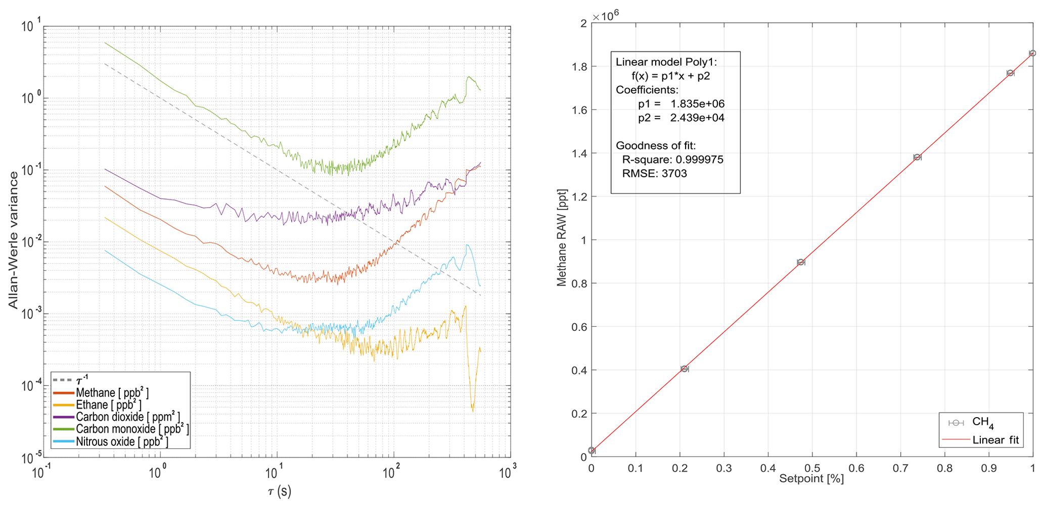
Figure 7Allan–Werle variance for all measured chemical species during ground-based operation (a). Panel (b) demonstrates linearity for methane is within achievable error bounds during ground-based operation using the online calibration gas mixing system from Sect. 2.3.
These tests confirmed the presence of an ambient pressure dependence found in earlier studies (i.e., Pitt et al., 2016). Here, we show in-field, ground-based instrument checks conducted in Hangar N-159 at NASA Wallops Flight Facility, Wallops Island, USA, to ensure proper instrument operation and determine instrument precision. Electric current drawn from the aircraft remained under 50 A at all times and settled at approximately 40 A. The flow rate stabilized at 23 SLPM for a sample cell pressure regulated at 50.0±0.5 hPa (0.2 hPa precision at 5 Hz frequency). Typical precision (standard deviation for 1 s averaging) for ground-based operation is summarized in Table 2.
Figure 7 shows the Allan–Werle variance for common averaging times τ for the individual trace gases monitored. For most species, averaging up to 20 s will decrease the standard deviation of most of the signals before deteriorating effects (i.e., drift) occur. Figure 7 also addresses retrieved mole fraction linearity. Linearity checks have been carried out for all species using the calibration system described in Sect. 2.3. All retrieved species are linear within the achievable controlled mass flow uncertainties from Sect. 2.3. CH4 is used in Fig. 7 for demonstration purposes.

Figure 8Spectral shifts for the CH4–H2O fit window (a) and the CO2–CO–N2O fit window (b). Spectral stability during ground-based operation is in the range of cm−1.
Typical shift parameters (as introduced in Sect. 3) for ground-based operation are depicted in Fig. 8 for the CH4–H2O and CO2–CO–N2O fit windows. These shift parameters can be considered as a tracer for instrument stability for both lasers. Overall spectral stability is in the range of cm−1. The regular short-timed spikes with a period of ∼5 min result from switching from sample to calibration gas and vice versa. Apart from these well-timed spikes and expected low-frequency instability (due to thermal changes) on the laser's spectral output, high-frequency shifts are evident, including discontinuities. The source of these discontinuities remains unclear. They could be introduced by the software-based frequency lock mechanism, by instabilities of the laser itself or by timing changes in the sampling. A software-based frequency lock refers to a controller regulating the laser temperature to compensate for drifts using the spectral shift as the controller input and the current to the Peltier as the controller output. The controller itself is implemented in software on the data analysis computer. The shape of the individual shifts match and so does their trend over time, which is a good indicator for a stable tuning rate during ground-based operation.

Figure 9A typical flight during ACT-America. This figure shows the flight pattern for 3 October 2017 with color-coded altitude. The flight includes two low-altitude (≈300 m a.g.l.) legs downwind and upwind of parts of the Marcellus shale area. High-altitude transects between the two low-altitude legs include two en route descents and ascents in West Virginia. Fair weather conditions and light southerly winds were present throughout the flight domain.
The instrument was successfully operated during 18 research flights aboard NASA Wallops Flight Facility's C-130 within the framework of the ACT-America fall 2017 field campaign. Other instrumentation in the ACT-America payload provided an excellent opportunity for instrument intercomparison. In situ CH4, CO2 and CO were measured using a Picarro G2401-m cavity ring-down spectrometer, and in situ CO2, CH4 and H2O (g) were measured using a Picarro G2301-m cavity ring-down analyzer. Both cavity ring-down instruments are anchored to WMO X2007 for CO2 (Zhao and Tans, 2006), WMO X2004A for CH4 (Dlugokencky et al., 2005) and WMO X2014A for CO (Baer et al., 2002). Precise C2H6 measurements were obtained by periodic flask samples by NOAA ESRL. Three onboard lidars and in situ sensors measuring the meteorological state variables – winds, temperature, pressure and water vapor – completed the C130s instrument suite. Here we present data from a typical flight (3 October 2017) to demonstrate the airborne instrument performance through intercomparison with well-established measurement techniques: the cavity ring-down greenhouse gas analyzers and flask samples.
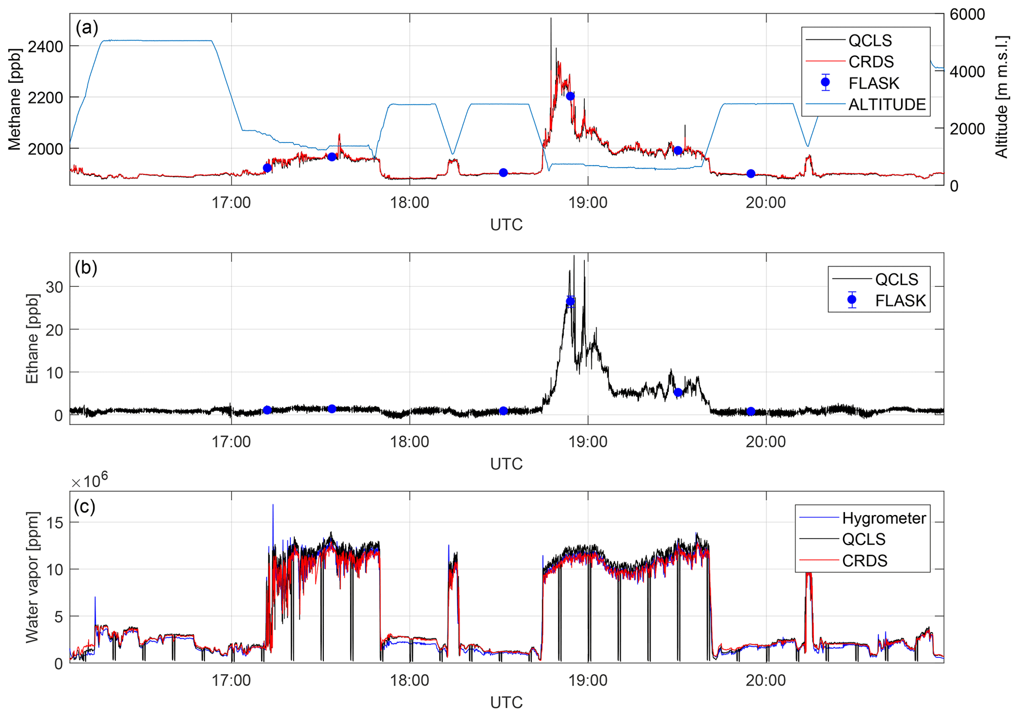
Figure 10A direct comparison between dry-air mole fractions retrieved from different measurement techniques for a complete flight on 3 October 2017. Depicted are methane (a), ethane (b) and water vapor (c) mole fractions. QCLS-retrieved methane data match with CRDS and flask data to within 1.4 ppb (1σ) and 3.9 ppb (1σ), respectively, after correcting for a constant bias. QCLS-retrieved ethane data agree with flask data to within 0.4 ppb (1σ). Water vapor sensed by an onboard dew-point hygrometer does differ from the CRDS and QCLS data.
As depicted in Fig. 9, the flight starts off from the eastern USA (Wallops Flight Facility, Virginia). A high-altitude transect to West Virginia is followed by two low-altitude legs downwind and upwind of parts of the Marcellus shale area: a large shale gas extraction region. The transects between the two low-altitude legs are flown at high altitude to facilitate nadir lidar observation, with two descents and ascents near the center en route.
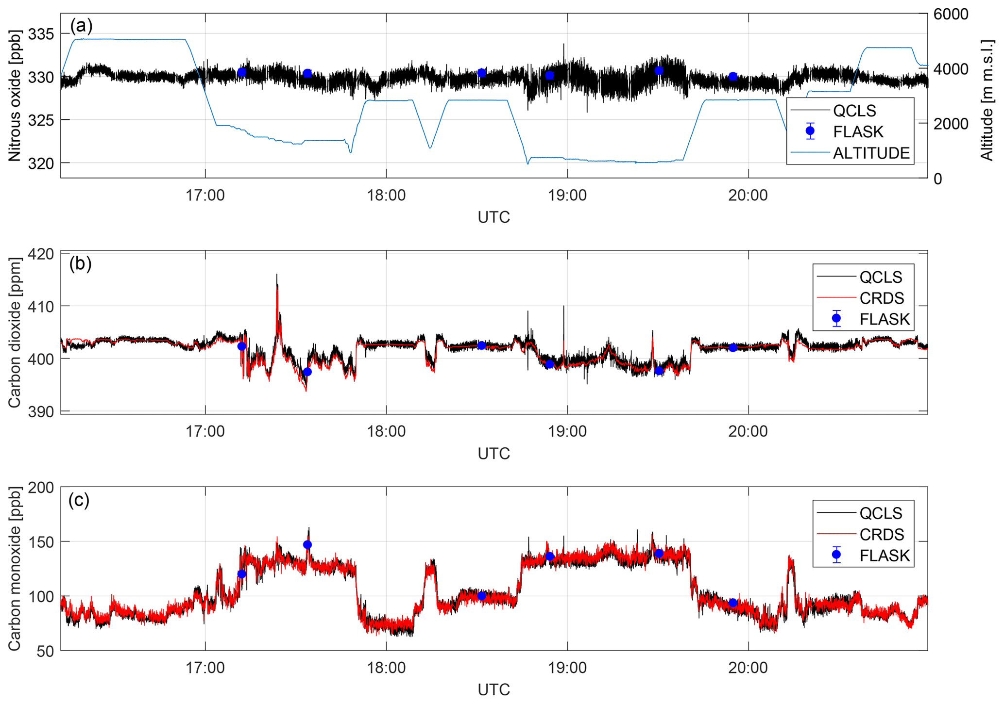
Figure 11Dry-air mole fractions retrieved from different measurement techniques for a complete flight on 3 October 2017. Depicted are nitrous oxide (a), carbon dioxide (b) and carbon monoxide (c) mole fractions.
Figure 10 depicts dry-air mole fractions for CH4, C2H6 and H2O measured by the different instruments during the 5 h flight. This figure provides evidence that the QCLS and CRDS methane data agree to within 1.4 ppb (1σ) over the entire flight. QCLS and flask methane data agree to within 3.9 ppb (1σ). It should be noted that care must be taken when interpreting the differences between slow flask samples and fast in situ measurements for high-variability flight segments. Figure 10b depicts the QCLS-retrieved C2H6 data superimposed with flask measurements. Here the QCLS-retrieved ethane data match the flask measurements (blue dots) to within 0.4 ppb (1σ). Unlike the QCLS, cavity ring-down and flask data are both sampled through an upstream dryer. These were computed by interpolating QCLS data to the flask end fill times. Figure 10c provides water vapor mole fractions obtained by an onboard dew-point hygrometer, from the G2301-m analyzer and from the QCLS. The QCLS water vapor data are used to correct for water vapor effects during the retrieval of dry-air mole fractions from the QCLS raw spectra as described in Sect. 3. By taking a closer look at panels a and b, the benefit of simultaneously measuring several species can be readily identified. Figure 10 shows enhanced CH4 without coinciding C2H6 enhancements for the first low-altitude leg. For the second low-altitude leg above the Marcellus area, however, concurrent CH4 and C2H6 enhancements suggest that natural gas is the dominant source.
Time series for the species N2O, CO and CO2 are shown in Fig. 11. The data obtained are comparable within instrument uncertainties. The N2O time series matches available flask data to within ±1.1 ppb. The CO2 absorption is retrieved from a molecular transition of the 13C16O2 carbon dioxide isotopologue and scaled with its natural abundance of approximately 1.1 % (Gordon et al., 2017) to report total CO2. Despite the much lower abundance compared to 12C16O2, the QCLS-retrieved CO2 data coincide with cavity ring-down data to within ±0.6 ppm (1σ) after correcting for a constant bias (see below). QCLS-retrieved CO mole fractions (Fig. 10b) agree with CRDS-retrieved data to within ±5 ppb (1σ). Figure 11 suggests that in-flight precision depends on whether the aircraft is flying within the planetary boundary layer (PBL) or above it. This is due to aircraft vibration excited by running engines and turbulence propagating into the instrument optics inducing slight changes in optical alignment and enhanced natural variability in the planetary boundary layer. We identified temperature fluctuations within ∼0.3 K, pressure changes of up to ∼200 hPa and relative humidity changes of up to 35 % in the instrument's optical compartment during this flight.
Table 3Typical in-flight performance including contributions to overall uncertainty. The total measurement uncertainty at 1 s temporal resolution is given by the quadrature sum of the individual contributors. Due to the lack of appropriate NOAA standards during the deployment, the uncertainties in C2H6, CO and N2O include combined uncertainties from concurrently measuring instruments (CRDS and FLASKS). The total uncertainties stated for these species do therefore not reflect the intrinsic uncertainties of the instrument, but rather worst-case values, that may have been better given the availability of appropriate standards. The WMO compatibility goals for Global Atmosphere Watch network compatibility among laboratories and central facilities have been added for completeness.
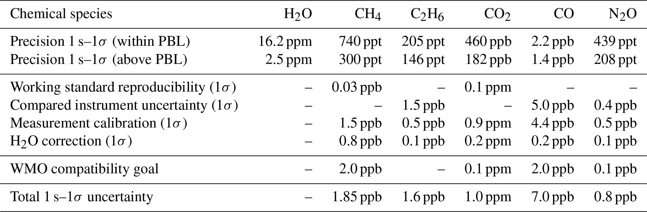
Typical in-flight precision figures based on ambient measurements at stable conditions for both regimes (standard deviation for 1s averaging) are summarized in Table 3. Total measurement uncertainty can be estimated from the uncertainty of the working standards, the uncertainty of calibration sequence evaluation, the uncertainty introduced by the H2O correction, the precision of the instrument and errors due to drift. We found a bias constant for the whole measurement series of ppb for CH4 and ppm for CO2 between the QCLS and CRDS–FLASK datasets. This constant bias has been corrected for. The origin of the biases is not yet fully understood. It was suggested that water vapor correction could have an impact on this. The reason for this assumption is that the calibration standards are always dry, whereas sampled air is not dried before entering the sample cell. Correlation plots however show no significant influence of water vapor on the residuals between the dry-air-sampling CRDS and the QCLS. It is therefore very unlikely that the water vapor correction is the source of the large bias in CO2. Instead we identified the difference in isotopic composition of the calibration standard versus sampled atmospheric air as the most probable cause. In this study we used working standards of synthetic nature from Air Liquide. Usually these are produced with CO2 from natural gas and oil combustion processes. We determined the CH4 and CO2 values of each working standard gas cylinder using a NOAA-anchored (Cert.-Nr. CB11361) Picarro G-1301-m. This has the drawback that we do not know the isotopic composition of our working standards as its impact had been considered negligible, e.g., Chen et al. (2010). We learned during the development of JFIT that the instrument uses a 13C16O2 line to derive ambient CO2. We estimate the required isotopic composition that could explain the large bias of 10 ppm (see Sect. S3 in the Supplement) in CO2 to be 98.447 % primary isotopologue and 1.079 % secondary isotopologue or ‰, which seems reasonable according to Coplen et al. (2002). Since we are reporting retrieved mole fractions relative to the WMO scale, only the working standard reproducibility contributes to the total uncertainty of CH4. Comparability of CO2 is difficult to assess here because of the unknown isotopic composition in our working standards. Uncertainty in the other measured species is taken from the ACT-America dataset to allow for WMO traceability. Due to the lack of appropriate NOAA standards during the deployment, the uncertainties in C2H6, CO and N2O include uncertainties reported in the ACT-America dataset from concurrently measuring instruments (CRDS and FLASKS). The total uncertainties stated for these species do therefore not reflect the intrinsic uncertainties of the instrument, but rather worst-case values, that may have been better given the availability of appropriate standards in future deployments. The uncertainty of calibration sequence evaluation (see Sect. 2.3) is estimated to be double the measurement precision, and the uncertainty introduced by the H2O correction is estimated from Eq. (1) using an assumed relative error on retrieved water vapor of 2 %. Errors originating from instrument drift are considered negligible due to our frequent calibration strategy (see Sect. 2.3). The total uncertainty is given by the quadrature sum of the individual contributors, listed in Table 3. Table 3 further includes the WMO compatibility goals for Global Atmosphere Watch (GAW) network compatibility among laboratories and central facilities. Precision/uncertainty figures given in Table 3 can be compared to 2 s–1σ PICARRO G2401-m airborne precision/uncertainty estimates based on ambient measurements at stable conditions of 0.3/2 ppb, 0.02/0.1 ppm and 2.0/5 ppb for CH4, CO2 and CO, respectively.
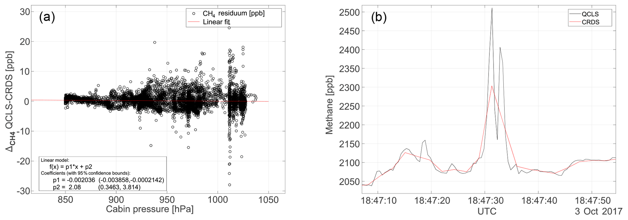
Figure 12Panel (a) shows the cabin pressure dependence for a typical flight on 3 October 2017. The large cabin pressure dependence in excess of 0.3 ppb hPa−1 reported by Pitt et al. (2016) has effectively been minimized using the calibration strategy from Sect. 2.3. Panel (b) shows a temporal zoom on the CH4 mole fractions at 18:47 UTC to emphasize the benefit of high-frequency measurements.
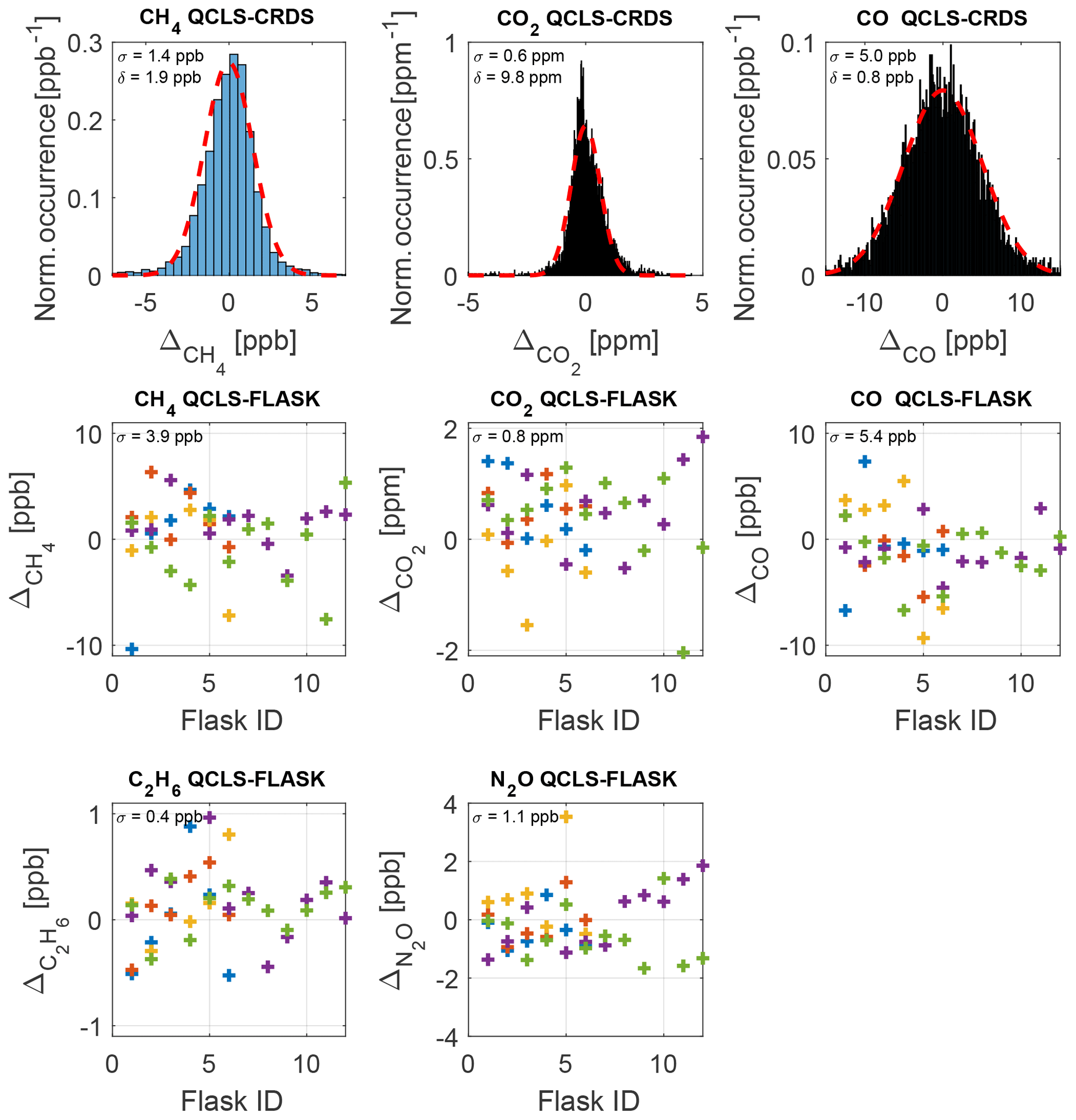
Figure 13Comparison of QCLS derived mole fractions to well-established in-flight cavity ring-down data and flask samples after correcting for a bias (δ) constant for the whole measurement series including standard deviations σ. Interpretation of the errors against flask samples is difficult for high-variability flight segments, due to the large flask sampling time. The residual plots show color-coded data from five typical flights on 3 October 2017 (blue), 11 October 2017 (red), 14 October 2017 (yellow), 18 October 2017 (violet) and 20 October 2017 (green).
A severe cabin pressure dependence in excess of 0.3 ppb hPa−1 in the CH4 mole fraction has been previously reported for airborne TILDAS instrumentation (Pitt et al., 2016). This instrumentation however physically differs from the one reported in this study. It is not possible to accurately compare the dependencies of one instrument relative to another since many factors and quantities involved are instrument-specific, e.g., the open-path length, the positioning and properties of optical elements, like windows and mirrors, and the stiffness and thermal expansion coefficient of the employed optical stands. We were nevertheless able to effectively minimize cabin pressure dependencies during operation of the QCLS instrument aboard the C130 using the calibration strategy from Sect. 2.3. This required a total calibration gas amount of ∼3.5 m3 (excluding zero air) for the 18 research flights. Figure 12a shows the difference in CH4 dry-air mole fraction reported by the QCLS and the CRDS as a function of cabin pressure during the research flight described above. The large scatter results from different sampling patterns among the two instruments hindering a one-to-one comparison of the QCLS measurements with the CRDS. While the QCLS samples continuously with a frequency of 2 Hz (1.5 kHz sweep frequency), the CRDS samples with a frequency of 0.5 Hz one species after the other. For CH4, for example, the CRDS uses the first 0.5 s of the 2 s sampling time, implying that, for the later 1.5 s, the CRDS is insensitive to CH4. Therefore, it is difficult to mimic the cavity ring-down sampling by averaging the QCLS data as would be required for a one-to-one comparison. Instead we decided to linearly interpolate QCLS data to the CRDS timescale. The fast response time of the QCLS instrument allows for better sampling of spatially narrow plumes, as can be seen from Fig. 12b. This panel zooms in on a relevant portion of the methane data from Fig. 10 and demonstrates that two mutually separated plumes can be identified from the high-frequency QCLS data at 18:47 UTC, for which only a single enhancement can be seen from cavity ring-down data. Furthermore, absolute enhancement and area beneath the peak(s) differ for the two instruments due to the different sampling patterns. Figure 13 compares the QCLS mole fractions to the cavity ring-down instrument and to the flask samples after correcting for a bias constant for the whole measurement series. The upper panels show differences in retrieved mole fractions between the QCLS and the cavity ring-down instrument for the flight on 3 October 2017, exhibiting a near-normal distribution. This hints towards residuals originating from random processes, i.e., noise. Despite the different sampling time and pattern, the measurements exhibit a compatibility to the calibrated cavity ring-down observations of 1.4 ppb in CH4, 0.6 ppm in CO2 and 5.0 ppb in CO.
Although interpretation of the differences to flask samples is difficult for high-variability flight segments, the lower panels of Fig. 13 show a good agreement for five typical flights (3, 11, 14, 18, 20 October 2017) during the ACT-America campaign. The relative deviations are in good agreement with the QCLS–CRDS data, except for CH4, where QCLS–CRDS compatibility (1.4 ppb) differs from the QCLS–FLASK compatibility of 3.9 ppb. This could be related to the different sampling times between the QCLS and flask samples.
We adapted the commercially available QCL- and ICL-based Dual Laser Trace Gas Monitor from Aerodyne Research Inc. (Billerica, USA) for airborne flux estimation (e.g., via the mass balance approach) and demonstrate successful operation for representative research flights aboard NASA Wallops Flight Facility's C-130 during the ACT-America field campaign in fall 2017. Known cabin pressure dependencies (Gvakharia et al., 2018; Pitt et al., 2016) on the retrieved mole fractions are effectively minimized using a frequent (5 to 10 min interval) two-point calibration approach obtained by flushing the sample cell with zero and target gases. This allows for a measurement duty cycle of ≥90 % when operating at sample flow rates near 23 SLPM. A custom retrieval software has been developed to learn about possible error sources and mitigation possibilities of instrument dependencies and to be able to extend the instruments capabilities in the future. Apart from low-frequency laser instability, we identify high-frequency “jumps” on the spectral axis, possibly due to the instruments frequency lock mechanism. In-flight performance has been assessed using data obtained during the research flight on the 3 October 2017 above the eastern USA. We identify two precision regimes whether flying within the planetary boundary layer or above, due to aircraft vibration propagating into the instrument optics and related slight changes in optical alignment. Typical in-flight precision figures for boundary layer flights (standard deviation for 1 s averaging) are 740 ppt, 205 ppt, 460 ppb, 2.2 ppb, 137 ppt and 16 ppm for CH4, C2H6, CO2, CO, N2O and H2O respectively. Precision figures improve by approximately a half for flights above the PBL. We estimate a total measurement uncertainty of 1.85 ppb, 1.6 ppb, 1.0 ppm, 7.0 ppb and 0.8 ppb in CH4, C2H6, CO2, CO and N2O, respectively. We demonstrate QCLS comparisons to concurrent flask sample and cavity ring-down measurements within combined measurement uncertainty for all targeted species. The instrument retrieves carbon dioxide mole fractions via a 13C16O2 absorption line. We find that precise knowledge of the δ13C of the working standards and the sampled air is needed to enhance CO2 compatibility when operating on the 2227.604 cm−1 13C16O2 absorption line.
Software code and data are available from the authors upon request.
The supplement related to this article is available online at: https://doi.org/10.5194/amt-12-1767-2019-supplement.
The authors declare that they have no conflict of interest.
We thank DLR VO-R for funding the young investigator research group
“Greenhouse Gases”. We also acknowledge funding from BMBF under project
“AIRSPACE” (grant no. FKZ01LK170). The Atmospheric Carbon and Transport (ACT)
– America project is a NASA Earth Venture Suborbital 2 project funded by
NASA's Earth Science Division (grant no. NNX15AG76G to Penn State). Aircraft
operations and US investigators were funded via the ACT-America project. We
greatly appreciate continuous support from Hans Schlager and Markus Rapp from
DLR. We further thank the GLORIA team, especially Christof Piesch and Hans Nordmeyer
at the Karlsruhe Institute of Technology (KIT), for enabling us
to pressure test the rack-mounted QCLS in a climate chamber. We also thank
Paul Stock and Monika Scheibe from DLR and Martin Nowicki from NASA WFF for
engineering support. Furthermore we would like to thank everyone involved
during the ACT-America field campaigns for their relentless dedication and
the helpful discussions, especially Alan Fried, Bing Lin, John Nowak,
Linda D. Thompson and Charles E. Juenger. Special thanks are given to Mark Zahniser and Dave Nelson
from Aerodyne Inc. for their valuable support whenever help was
needed.
The article processing charges for this open-access
publication were covered by a Research
Centre of the Helmholtz Association.
This paper was edited by Christof Janssen and reviewed by Alan Fried and three anonymous referees.
Abrarov, S. and Quine, B.: A Rational Approximation for Efficient Computation of the Voigt Function in Quantitative Spectroscopy, J. Math. Res., 7, https://doi.org/10.5539/jmr.v7n2, 2015. a
Baer, D., Paul, J., Gupta, M., and O'Keefe, A.: Sensitive absorption measurements in the near-infrared region using off-axis integrated-cavity-output spectroscopy, Appl. Phys. B, 75, 261–265, https://doi.org/10.1007/s00340-002-0971-z, 2002. a
Barkley, Z. R., Lauvaux, T., Davis, K. J., Deng, A., Miles, N. L., Richardson, S. J., Cao, Y., Sweeney, C., Karion, A., Smith, M., Kort, E. A., Schwietzke, S., Murphy, T., Cervone, G., Martins, D., and Maasakkers, J. D.: Quantifying methane emissions from natural gas production in north-eastern Pennsylvania, Atmos. Chem. Phys., 17, 13941–13966, https://doi.org/10.5194/acp-17-13941-2017, 2017. a
Beck, M., Hofstetter, D., Aellen, T., Faist, J., Oesterle, U., Ilegems, M., Gini, E., and Melchior, H.: Continuous Wave Operation of a Mid-Infrared Semiconductor Laser at Room Temperature, Science, 295, 301–305, https://doi.org/10.1126/science.1066408, 2002. a
Cambaliza, O. L. M., Shepson, P., Bogner, J., Caulton, R. D., Stirm, B., Sweeney, C., Montzka, A. S., Gurney, K., Spokas, K., Salmon, O., Lavoie, T., Hendricks, A., Mays, K., Turnbull, J., Miller, R. B., Lauvaux, T., Davis, K., Karion, A., Moser, B., and Richardson, S.: Quantification and source apportionment of the methane emission flux from the city of Indianapolis, Elementa-Science of the Anthropocene, 3, 000037, https://doi.org/10.12952/journal.elementa.000037, 2015. a
Capasso, F.: High-performance midinfrared quantum cascade lasers, J. Opt. Eng., 49, 111102, https://doi.org/10.1117/1.3505844, 2010. a
Catoire, V., Robert, C., Chartier, M., Jacquet, P., Guimbaud, C., and Krysztofiak, G.: The SPIRIT airborne instrument: a three-channel infrared absorption spectrometer with quantum cascade lasers for in situ atmospheric trace-gas measurements, Appl. Phys. B, 123, 244, https://doi.org/10.1007/s00340-017-6820-x, 2017. a
Chen, H., Winderlich, J., Gerbig, C., Hoefer, A., Rella, C. W., Crosson, E. R., Van Pelt, A. D., Steinbach, J., Kolle, O., Beck, V., Daube, B. C., Gottlieb, E. W., Chow, V. Y., Santoni, G. W., and Wofsy, S. C.: High-accuracy continuous airborne measurements of greenhouse gases (CO2 and CH4) using the cavity ring-down spectroscopy (CRDS) technique, Atmos. Meas. Tech., 3, 375–386, https://doi.org/10.5194/amt-3-375-2010, 2010. a, b
Ciais, P., Sabine, C., Bala, G., Bopp, L., Brovkin, V., Canadell, J., Chhabra, A., DeFries, R., Galloway, J., Heimann, M., Jones, C., Le Quéré, C., Myneni, R., Piao, S., and Thornton, P.: Carbon and Other Biogeochemical Cycles, book section 6, 465–570, Cambridge University Press, Cambridge, United Kingdom and New York, NY, USA, https://doi.org/10.1017/CBO9781107415324.015, 2013. a
Coplen, T. B., Bohlke, J., De Bièvre, P., Ding, T., Holden, N., Hopple, J., R. Krouse, H., Lamberty, A., Peiser S. H., Révész, K., Rieder, E. S., and Rosman, J. R. K.: Isotope-abundance Variations of Selected Elements (IUPAC Technical Report), Pure Appl. Chem., 74, 1987–2017, https://doi.org/10.1351/pac200274101987, 2002. a
Dlugokencky, E. J., Myers, R. C., Lang, P. M., Masarie, K. A., Crotwell, A. M., Thoning, K. W., Hall, B. D., Elkins, J. W., and Steele, L. P.: Conversion of NOAA atmospheric dry air CH4 mole fractions to a gravimetrically prepared standard scale, J. Geophys. Res.-Atmos., 110, D18, https://doi.org/10.1029/2005JD006035, 2005. a, b
Filges, A., Gerbig, C., Chen, H., Franke, H., Klaus, C., and Jordan, A.: The IAGOS-core greenhouse gas package: a measurement system for continuous airborne observations of CO2, CH4, H2O and CO, Tellus B, 67, 27989, https://doi.org/10.3402/tellusb.v67.27989, 2015. a
Fried, A. and Richter, D.: Infrared Absorption Spectroscopy, chap. 2, pp. 72–146, John Wiley & Sons, Ltd, https://doi.org/10.1002/9780470988510.ch2, 2007. a
Gordon, I., Rothman, L., Hill, C., Kochanov, R., Tan, Y., Bernath, P., Birk, M., Boudon, V., Campargue, A., Chance, K., Drouin, B., Flaud, J.-M., Gamache, R., Hodges, J., Jacquemart, D., Perevalov, V., Perrin, A., Shine, K., Smith, M.-A., Tennyson, J., Toon, G., Tran, H., Tyuterev, V., Barbe, A., Császár, A., Devi, V., Furtenbacher, T., Harrison, J., Hartmann, J.-M., Jolly, A., Johnson, T., Karman, T., Kleiner, I., Kyuberis, A., Loos, J., Lyulin, O., Massie, S., Mikhailenko, S., Moazzen-Ahmadi, N., Müller, H., Naumenko, O., Nikitin, A., Polyansky, O., Rey, M., Rotger, M., Sharpe, S., Sung, K., Starikova, E., Tashkun, S., Auwera, J. V., Wagner, G., Wilzewski, J., Wcisło, P., Yu, S., and Zak, E.: The HITRAN2016 molecular spectroscopic database, J. Quant. Spectrosc. Ra., 203, 3–69, https://doi.org/10.1016/j.jqsrt.2017.06.038, 2017. a, b
Gvakharia, A., Kort, E. A., Smith, M. L., and Conley, S.: Testing and evaluation of a new airborne system for continuous N2O, CO2, CO, and H2O measurements: the Frequent Calibration High-performance Airborne Observation System (FCHAOS), Atmos. Meas. Tech., 11, 6059–6074, https://doi.org/10.5194/amt-11-6059-2018, 2018. a, b, c
Harazono, Y., Iwata, H., Sakabe, A., Ueyama, M., Takahashi, K., Nagano, H., Nakai, T., and Kosugi, Y.: Effects of water vapor dilution on trace gas flux, and practical correction methods, J. Agric. Meteorol., 71, 65–76, https://doi.org/10.2480/agrmet.D-14-00003, 2015. a
Harrison, J. J., Allen, N. D., and Bernath, P. F.: Infrared absorption cross sections for ethane (C2H6) in the 3 µm region, J. Quant. Spectrosc. Ra., 111, 357–363, https://doi.org/10.1016/j.jqsrt.2009.09.010, 2010. a
Kim, M., Bewley, W. W., Canedy, C. L., Kim, C. S., Merritt, C. D., Abell, J., Vurgaftman, I., and Meyer, J. R.: High-power continuous-wave interband cascade lasers with 10 active stages, Opt. Express, 23, 9664–9672, https://doi.org/10.1364/OE.23.009664, 2015. a
Klemm, O., Hahn, M. K., and Giehl, H.: Airborne, Continuous Measurement of Carbon Monoxide in the Lower Troposphere, Environ. Sci. Technol., 30, 115–120, https://doi.org/10.1021/es950145j, 1996. a
Kooijmans, L. M. J., Uitslag, N. A. M., Zahniser, M. S., Nelson, D. D., Montzka, S. A., and Chen, H.: Continuous and high-precision atmospheric concentration measurements of COS, CO2, CO and H2O using a quantum cascade laser spectrometer (QCLS), Atmos. Meas. Tech., 9, 5293–5314, https://doi.org/10.5194/amt-9-5293-2016, 2016. a
Marquardt, D.: An Algorithm for Least-Squares Estimation of Nonlinear Parameters, J. Soc. Ind. Appl. Math., 11, 431–441, https://doi.org/10.1137/0111030, 1963. a
McManus, J. B., Zahniser, M. S., and Nelson, D. D.: Dual quantum cascade laser trace gas instrument with astigmatic Herriott cell at high pass number, Appl. Optics, 50, A74–A85, https://doi.org/10.1364/AO.50.000A74, 2011. a, b
McManus, J. B., Nelson, D. D., and Zahniser, M. S.: Design and performance of a dual-laser instrument for multiple isotopologues of carbon dioxide and water, Opt. Express, 23, 6569–6586, https://doi.org/10.1364/OE.23.006569, 2015. a
O'Shea, S. J., Allen, G., Fleming, Z. L., Bauguitte, S. J., Percival, C. J., Gallagher, M. W., Lee, J., Helfter, C., and Nemitz, E.: Area fluxes of carbon dioxide, methane, and carbon monoxide derived from airborne measurements around Greater London: A case study during summer 2012, J. Geophys. Res.-Atmos., 119, 4940–4952, https://doi.org/10.1002/2013JD021269, 2013. a
Peischl, J., Karion, A., Sweeney, C., Kort, E. A., Smith, M. L., Brandt, A. R., Yeskoo, T., Aikin, K. C., Conley, S. A., Gvakharia, A., Trainer, M., Wolter, S., and Ryerson, T. B.: Quantifying atmospheric methane emissions from oil and natural gas production in the Bakken shale region of North Dakota, J. Geophys. Res.-Atmos., 121, 6101–6111, https://doi.org/10.1002/2015JD024631, 2015. a
Pitt, J. R., Le Breton, M., Allen, G., Percival, C. J., Gallagher, M. W., Bauguitte, S. J.-B., O'Shea, S. J., Muller, J. B. A., Zahniser, M. S., Pyle, J., and Palmer, P. I.: The development and evaluation of airborne in situ N2O and CH4 sampling using a quantum cascade laser absorption spectrometer (QCLAS), Atmos. Meas. Tech., 9, 63–77, https://doi.org/10.5194/amt-9-63-2016, 2016. a, b, c, d, e
Ravishankara, A. R., Daniel, J. S., and Portmann, R. W.: Nitrous Oxide (N2O): The Dominant Ozone-Depleting Substance Emitted in the 21st Century, Science, 326, 123–125, https://doi.org/10.1126/science.1176985, 2009. a
Richter, D., Weibring, P., Walega, J. G., Fried, A., Spuler, S. M., and Taubman, M. S.: Compact highly sensitive multi-species airborne mid-IR spectrometer, Appl. Phys. B, 119, 119–131, https://doi.org/10.1007/s00340-015-6038-8, 2015. a
Rothman, L. S., Gordon, I. E., Babikov, Y., Barbe, A., Chris Benner, D., Bernath, P. F., Birk, M., Bizzocchi, L., Boudon, V., Brown, L. R., Campargue, A., Chance, K., Cohen, E. A., Coudert, L. H., Devi, V. M., Drouin, B. J., Fayt, A., Flaud, J.-M., Gamache, R. R., Harrison, J. J., Hartmann, J.-M., Hill, C., Hodges, J. T., Jacquemart, D., Jolly, A., Lamouroux, J., Le Roy, R. J., Li, G., Long, D. A., Lyulin, O. M., Mackie, C. J., Massie, S. T., Mikhailenko, S., Müller, H. S. P., Naumenko, O. V., Nikitin, A. V., Orphal, J., Perevalov, V., Perrin, A., Polovtseva, E. R., Richard, C., Smith, M. A. H., Starikova, E., Sung, K., Tashkun, S., Tennyson, J., Toon, G. C., Tyuterev, V. G., and Wagner, G.: The HITRAN2012 molecular spectroscopic database, J. Quant. Spectros. Ra., 130, 4–50, https://doi.org/10.1016/j.jqsrt.2013.07.002, 2013. a
Santoni, G. W., Daube, B. C., Kort, E. A., Jiménez, R., Park, S., Pittman, J. V., Gottlieb, E., Xiang, B., Zahniser, M. S., Nelson, D. D., McManus, J. B., Peischl, J., Ryerson, T. B., Holloway, J. S., Andrews, A. E., Sweeney, C., Hall, B., Hintsa, E. J., Moore, F. L., Elkins, J. W., Hurst, D. F., Stephens, B. B., Bent, J., and Wofsy, S. C.: Evaluation of the airborne quantum cascade laser spectrometer (QCLS) measurements of the carbon and greenhouse gas suite – CO2, CH4, N2O, and CO – during the CalNex and HIPPO campaigns, Atmos. Meas. Tech., 7, 1509–1526, https://doi.org/10.5194/amt-7-1509-2014, 2014. a, b
Simpson, I. J., Sulbaek Andersen, M. P., Meinardi, S., Bruhwiler, L., Blake, N. J., Helmig, D., Rowland, F. S., and Blake, D. R.: Long-term decline of global atmospheric ethane concentrations and implications for methane, Nature, 488, 490 EP, https://doi.org/10.1038/nature11342, 2012. a
Smith, M. L., Kort, E. A., Karion, A., Sweeney, C., Herndon, S. C., and Yacovitch, T. I.: Airborne Ethane Observations in the Barnett Shale: Quantification of Ethane Flux and Attribution of Methane Emissions, Environ. Sci. Technol., 49, 8158–8166, https://doi.org/10.1021/acs.est.5b00219, 2015. a, b
Vurgaftman, I., Weih, R., Kamp, M., Meyer, J. R., Canedy, C. L., Kim, C. S., Kim, M., Bewley, W. W., Merritt, C. D., Abell, J., and Höfling, S.: Interband cascade lasers, J. Phys. D, 48, 123001, https://doi.org/10.1088/0022-3727/48/12/123001, 2015. a
Zellweger, C., Emmenegger, L., Firdaus, M., Hatakka, J., Heimann, M., Kozlova, E., Spain, T. G., Steinbacher, M., van der Schoot, M. V., and Buchmann, B.: Assessment of recent advances in measurement techniques for atmospheric carbon dioxide and methane observations, Atmos. Meas. Tech., 9, 4737–4757, https://doi.org/10.5194/amt-9-4737-2016, 2016. a
Zhao, C. L. and Tans, P. P.: Estimating uncertainty of the WMO mole fraction scale for carbon dioxide in air, J. Geophys. Res.-Atmos., 111, D8, https://doi.org/10.1029/2005JD006003, 2006. a, b