the Creative Commons Attribution 4.0 License.
the Creative Commons Attribution 4.0 License.
 | 04 Apr 2019
Optimal estimation method retrievals of stratospheric ozone profiles from a DIAL
Ghazal Farhani
Robert J. Sica
Sophie Godin-Beekmann
Alexander Haefele
This paper provides a detailed description of a first-principle optimal estimation method (OEM) applied to ozone retrieval analysis using differential absorption lidar (DIAL) measurements. The air density, detector dead times, background coefficients, and lidar constants are simultaneously retrieved along with ozone density profiles. Using an averaging kernel, the OEM provides the vertical resolution of the retrieval as a function of altitude. A maximum acceptable height at which the a priori has a small contribution to the retrieval is calculated for each profile as well. Moreover, a complete uncertainty budget including both systematic and statistical uncertainties is given for each individual retrieved profile. Long-term stratospheric DIAL ozone measurements have been carried out at the Observatoire de Haute-Provence (OHP) since 1985. The OEM is applied to three nights of measurements at OHP during an intensive ozone campaign in July 2017 for which coincident lidar–ozonesonde measurements are available. The retrieved ozone density profiles are in good agreement with both traditional analysis and the ozonesonde measurements. For the three nights of measurements, below 15 km the difference between the OEM and the sonde profiles is less than 25 %, and at altitudes between 15 and 25 km the difference is less than 10 %; the OEM can successfully catch many variations in ozone, which are detected in the sonde profiles due to its ability to adjust its vertical resolution as the signal varies. Above 25 km the difference between the OEM and the sonde profiles does not exceed 20 %.


Stratospheric ozone plays a critical role, allowing life to thrive on Earth by absorbing the ultraviolet (UV) radiation emitted by the Sun. Moreover, the temperature structure in the stratosphere is determined by the absorption of UV radiation by ozone, which is followed by the exothermic recombination of O2 and O. Thus, ozone is the main driver in defining the atmosphere's temperature structure (Andrews et al., 1987).
After observing a significant global depletion of stratospheric ozone (Farman et al., 1985; WMO, 2011, 2014), the Montreal Protocol was established as an international treaty to control and to halt the release of ozone-depleting substances (ODSs). As a result, the abundance of anthropogenic ODSs in the troposphere has decreased from its peak in 1994 by approximately 10 % (WMO, 2014). Recently, the first signs of stratospheric ozone recovery over Antarctica were observed (Solomon et al., 2016). However, for nonpolar regions since 2000, no significant positive trend has been detected (WMO, 2014).
Trends in ozone are of the order of a few percent per decade, e.g., in the upper stratosphere around +1 % to +3 % per decade (Harris et al., 2015). Although the trends in total column ozone are insignificant, in the upper stratosphere (around 40 km) the ozone level has significantly increased (Harris et al., 2015). This increase does not indicate that ozone in the whole stratosphere is increasing. In contrast, many studies have suggested that, at midlatitudes and tropical latitudes, the ozone content in the lower stratosphere has continued to decrease (Ball et al., 2018).
Thus, it is important to take ozone measurements with an instrument with high spatial and temporal resolution to detect these changes.
DIAL (differential absorption lidar) measures the vertical distribution of ozone density with high temporal and vertical resolution. In the DIAL technique, two laser beams at different wavelengths are simultaneously transmitted to the atmosphere. The spectral range for the laser beams is chosen in the UV range in which one of the wavelengths is highly absorbed by ozone and is called the “online” wavelength. The other wavelength has a relatively lower absorption by ozone and is called the “off-line” wavelength. As the ozone cross sections are well known, the differential lidar technique allows the absolute number density to be determined from the combination of the online and off-line measurements, without the need for external calibration.
Details of the DIAL technique can be found elsewhere (Schotland, 1974). The traditional analysis of DIAL ozone measurements was presented by Megie et al. (1985), McDermid et al. (1990), and Godin-Beekmann et al. (2003). Recently, Leblanc et al. (2016b) have presented a detailed review of the method with a full assessment of the random and systematic uncertainties. In this method, both statistical and systematic uncertainties are calculated. Moreover, count profiles from multichannel systems must be merged to generate a single profile from multiple channels.
To determine a single ozone profile, the optimal estimation method (OEM) uses photocounts from multiple channels, without merging or applying corrections. Recently, the OEM has been implemented to lidar measurements to retrieve aerosol backscatter profiles, Rayleigh temperature, and water vapor mixing ratio (Povey et al., 2014; Sica and Haefele, 2015, 2016). Here, we are applying the first principles of OEM to retrieve stratospheric ozone profiles from measurements at the Observatoire de Haute-Provence (OHP) located in France. Ozone profiles are retrieved from raw (Level 0) measurements of four digital channels, two high altitude and two low altitude.
Moreover, in this method, no prefiltering or post-filtering of retrievals is needed. The OEM provides a quantitative value for the maximum height of the retrieval. The uncertainty budget, including both random and systematic uncertainties, is calculated on a profile-by-profile basis.
This paper introduces a first-principle OEM retrieval for stratospheric ozone density from DIAL measurements. In Sect. 2, the traditional analysis of ozone retrievals is discussed in detail and compared with the OEM algorithm. In Sect. 3, the approach to implement the OEM to the OHP lidar measurements is discussed in detail. In Sect. 4, the OEM is applied to the night of 26 July 2017, and the result is compared with both ozonesonde measurements and the traditional analysis. The averaging kernel, vertical resolution of the retrieval, and systematic and statistical uncertainties of the retrieval are discussed as well. Moreover, the OEM results for two other nights are shown and compared with the traditional analysis. Section 5 is the summary and our future work plans.
2.1 The traditional DIAL method to determine ozone number density
In the DIAL technique, the measured backscattered photocounts, Nobs(z, λi), for a laser pulse at wavelength λi are given by the lidar equation (Fernald, 1984).
where C(λi) is the lidar constant, which contains the efficiency of the system, the telescope area, and the emitted number of photons at each wavelength, O(z) is the overlap function of the lidar, β(z, λi) is the atmospheric backscattering coefficient, τ(z, λi) is the atmospheric optical depth, and B(z) is the background photon counts. The atmospheric optical depth is given by
where z0 is the altitude of the station, is the ozone absorption cross section at the specific altitude and wavelength, T(z′) is the atmospheric temperature, is the ozone number density to be measured, α(λ, z) is the atmospheric extinction coefficient, which includes both Rayleigh and Mie scattering extinction coefficients, and ∑eσe(λ)ne(z) is the extinction by other absorbers (like SO2 and NO2). In major volcanic eruptions the abundance of SO2 gas in the stratosphere can significantly perturb ozone retrievals. However, SO2 only stays in the stratosphere for 30 to 40 d (Heath et al., 1983). In general, the amount of SO2 mixing ratio in the stratosphere is negligible. At midlatitudes, the uncertainty of ozone number density due to absorption by NO2 reaches a maximum of 0.4 % between 25 and 30 km of altitude. Thus, the effect of NO2 on ozone retrievals is not significant, and the third term of Eq. (1) is small (Brasseur et al., 1999; Godin-Beekmann et al., 2003).
For many lidar systems, at count rates below about 1 MHz, the relation between the true counts and the observed signal is linear. However, for higher counts, the detector's response may not be linear. This relation for the non-paralyzable detectors is
and for the paralyzable ones is
where Nobs is the observed counts, Ntrue is the true counts, and γ is the dead time. In the traditional method, the lidar measurements should be corrected for the effect of dead time. If the value of the dead time is not known, an empirical fit can be used to estimate the dead time value (Donovan et al., 1995). It is also well known that for high-intensity systems the output of the photomultiplier tube (PMT) can show an excess of counts some time after the signal intensity is maximum, a “tail” that is called signal-induced noise (SIN) (Hunt and Poultney, 1975). In fact, SIN is the residual signal originating from high signal intensities at low altitudes. It adds up with the background signal and is visible at altitudes at which the signal-to-noise ratio (SNR) is very small (Iikura et al., 1987). Using a mechanical chopper to block high-intensity light from approaching the detector is the most practical way to avoid SIN. It is important to consider the noise component from the upper altitude of lidar signals. In many lidars the background is a constant and the effect of SIN is not detected. If present, SIN is modeled using an exponential function of the form
where the fitting coefficients e, f, and g are analytically determined (Iikura et al., 1987). The SIN is more pronounced for the online wavelength, and for most nights its effect on the off-line wavelength is negligible; hence, a constant background can be used.
2.2 Ozone density retrievals
In the traditional method, the derivative of the ratio between the online and off-line signals is calculated. The ozone number density can be retrieved as follows:
where N(λ1, z) and N(λ2, z) are, respectively, the online and off-line signals at altitude z, B1(z) and B2(z) are the background signals, and (z) is the differential absorption cross section between the two wavelengths. is a correction term for the effect of differential Rayleigh and Mie scattering and the differential absorption by other absorbers. More details can be found in McDermid et al. (1990), Godin-Beekmann et al. (2003), and Leblanc et al. (2016b).
In the traditional ozone retrieval algorithm, several corrections are applied to the raw (Level 0) counts to produce corrected photocounts. For high count rates, the dead time of the counting system is determined and a nonlinearity correction is applied. Depending on the configuration of the lidar, channels with different gains may be merged (“glued”) to produce a single ozone profile. Determining the optimized height to merge the channels is typically done empirically. In the DIAL technique, the rapid decrease in sensitivity to ozone in the upper stratosphere is another important consideration. Low-pass filters are used to reduce the noise of the signals. For an ideal low-pass filter, the transfer function of all frequencies between 0 and the cutoff frequency, νc, is 1, and the transfer function from νc to 1 is 0, where the reduced frequency ν is defined as and fN is the Nyquist frequency. The final vertical resolution of the signal, Δzf, varies by the order of filter, which depends on the cutoff frequency and the initial vertical resolution Δzi:
A detailed discussion on the digital filtering and vertical resolution can be found in Godin et al. (1999) and Leblanc et al. (2016a).
In the lower stratosphere, perturbations in the ozone profiles are well detected; however, depending on the number of points in the filter (order of filter), the perturbation can be largely attenuated and cause negative or positive biases. For higher altitudes, because of the lower SNR, the vertical resolution is decreased. Different numerical filters have been tested to optimize ozone retrievals. In all these techniques, to overcome the SNR decrease, the number of coefficients in the filters is increased with altitude (Godin et al., 1999).
2.3 Applying the optimal estimation method to ozone retrievals
The OEM is an inverse method in which the Bayesian theorem is used to find the probability distribution function (PDF) of the state of interest. Let be the state vector and be the vector of the measurements. The relation between the measurements and the state vector is
where F(x, b) is called the forward model. The forward model describes our understanding of the physics of the measurements as well as the instrument's characteristics. Here, b is the model parameter vector, which contains additional parameters needed in the forward model, and the noise in the measurements is the vector ϵ. In lidar measurements, the photon counts follow a Poisson distribution. However, for a count rate greater than 10 to 20, the PDF of the corresponding error tends toward a Gaussian distribution. Therefore, using the Bayesian approach and assuming a Gaussian PDF for all quantities, for a given measurement y, the most likely state of x is found by minimizing the following cost function:
where Sy is the covariance matrix of the measurements, xa is the a priori profile, which is an initial guess for the state vector, and Sa is the associated a priori covariance matrix. Typically, the cost is normalized to the number of measurements, and a cost of around 1 indicates a good retrieval.
As the forward model is nonlinear, the Marquardt–Levenberg method is used to find the state vector. The optimized solution for the state vector x occurs when the following iteration converges.
Here, is the Jacobian of the forward model, and γi is a damping factor for the iteration. A comprehensive description of the application of the Marquardt–Levenberg method to OEM can be found in Rodgers (2000).
2.4 Ozone DIAL forward model
Our first-principle OEM retrieval uses the lidar equation as the forward model and the raw counts are the measurements. The lidar equation for the true counts is
where λon and λoff represent the online and off-line channels, and are, respectively, the ozone and atmospheric transmissions in each wavelength, and are the lidar constants, and and are the background counts. For the stratospheric ozone measurements, in the altitude region of retrieval, the overlap is complete, and thus we have not included it in our forward model. Depending on the characteristics of the data acquisition system, the true counts are related to the observed counts by either Eq. (1) or (2). In multichannel systems, our forward model calculates the online and off-line wavelengths for both high-altitude and low-altitude channels. The transmissions are defined as
where the optical depth is previously defined in Eq. (1). Both atmospheric optical depth and atmospheric backscattering coefficients have contributions due to scattering from molecules and aerosols:
where βair(z) and βaer(z) are the corresponding air and aerosol backscattering coefficients. The online and off-line coefficients are related through the following equation:
where for aerosols the Ångstrom coefficient a equals approximately 1, and for molecular scattering the Ångstrom coefficient a equals 4. In this paper, we only considered the clean-night condition. Therefore, the aerosol contribution to the process is not included, but it could be in the future.
Due to the presence of SIN in the online channel, the background is assumed to be a function of height in the form of Eq. (3), while due to a negligible presence of SIN in the off-line channel, a constant background is used. If necessary, it is possible and easy to assign any reasonable analytic function for the background in both channels. Therefore, if needed the background for the off-line channel can be assumed as a function of height as well. Using the above forward model, the ozone and air density profiles, the background coefficients, the dead time, and the lidar constants for the four channels are simultaneously retrieved. Other parameters in the forward model are treated as model parameters. Hence, they are fixed but considered a source of uncertainty on the retrieval (b model parameter uncertainty) contributing to the total uncertainty budget (see Table 1).
The statistical uncertainty of the retrieved quantities and the model parameter uncertainties are calculated as follows:
where Sm, Sf, Sb are the covariances of the retrieval noise, the forward model parameter error, and the error covariance of the model parameters. The gain matrix, , gives the sensitivity of the retrieval to the measurements, while is the Jacobian of the forward model with respect to b.
To find the optimized solution of Eq. (7), a priori profiles for ozone and air density, as well as a priori values for background counts, dead time, and lidar constants, are needed. Furthermore, b model parameter values and the covariance matrix of the measurements, a priori profiles, and model parameters need to be calculated. A summary of steps needed to implement the OEM for our ozone retrievals is shown in Fig. 1. A detailed description of these steps is provided in this section.
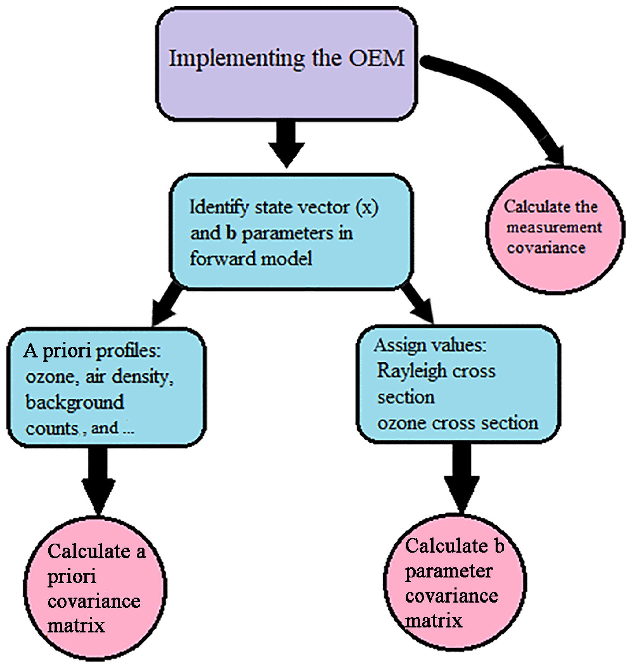
Figure 1To implement the OEM, the a priori profiles for ozone and air density, background counts, dead time values, and lidar constants are needed. Moreover, b parameters should be identified and proper values for them should be calculated. The covariance matrices for a priori profiles, measurements, and b parameters need to be calculated as well.
The a priori ozone profile used for all retrievals is from an OHP ozone climatology. The climatology contains monthly averaged ozone profiles using the last 30 years of OHP DIAL and SAGE II satellite overpass measurements. The variability of the climatology we use is 50 % at the 2σ level, encompassing 95 % of the variability and 10 % above 20 km of altitude. Alternatively, we have used the US standard model (Krueger and Minzner, 1976) as an a priori ozone profile, which yields similar results for our ozone retrievals.
In the traditional method, the ratio of the online to off-line channels is calculated. Thus, there is no need to assume an air density profile to retrieve ozone. However, in the correction term (Eq. 4), the air density profile is needed and an atmospheric model or a measurement is used. In the OEM, we are retrieving the air density as a state vector, and the Mass Spectrometer Incoherent Scatter Radar (MSIS) air density profile is used as the a priori profile. The MSIS profiles are generally in good agreement with the ozonesonde measurements of air density. An uncertainty of 15 % is assigned to the a priori of air density.
In the case of ozone and air density there is a vertical correlation between the elements of retrieval states. This corresponds to the off-diagonal elements of the a priori covariance matrix. The correlation length gives the vertical correlation between the retrieval elements. It can be difficult to quantify the vertical length of this correlation. We have used a correlation length (łs) of 1000 m for ozone at altitudes below 18 km and a correlation length of 1400 m at higher altitudes. The air density has a correlation length of 1400 m for all regions, which is about of a scale height, consistent with the vertical resolution of density measurements used for Rayleigh-scatter temperature lidar. It is beyond the range of this study, but feasible, that an extended ozonesonde record from a location could be used to better assess the correlation length for ozone density. The effect of using no correlation length would be to make the retrieval overly sensitive to measurement noise; using a very long correlation length would act to smooth the retrieval beyond the resolution of the retrieval grid. A tent function is used to model the decay of correlation (Eriksson et al., 2005).
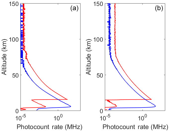
Figure 2Average count rates for 5 h of measurements on 26 July 2017. (a) Online wavelength (blue curve, low altitude; red curve, high altitude). (b) Off-line wavelength (blue curve, low altitude; red curve, high altitude).
For the off-line channel the mean of the counts above 80 km is taken as the a priori background, and their variance divided by the number of bins in the selected altitude region is used as the a priori uncertainty in the background counts. For the online channel, an exponential function in the form of Eq. (3) is fitted to counts above 80 km. The coefficients of the function are the a priori values. Depending on how good the initial fit is, uncertainties are assigned to the a priori coefficients, but for most nights a 20 % uncertainty is chosen.
Using the forward model, the a priori lidar constants for both channels were estimated and an initial standard deviation of 10 % for both channels is assigned. In a range in which photon-counting measurements are linear (or nonlinearity is correctable), Poisson statistics is applied. Thus, the measurement variances are the number of photons in each atmospheric layer located at altitude Δz, and there is no correlation between different layers (the off-diagonal elements of the matrix are zero).
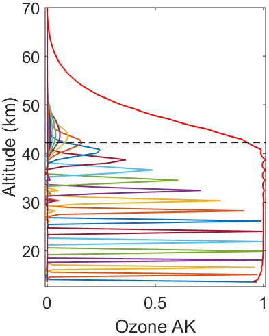
Figure 3Averaging kernels for the ozone density for the measurements on 26 July 2017. The horizontal dashed line is a height below which the OEM retrieval is more than 80 % due to the measurements. Above this horizontal cutoff as the SNR drops, the retrieval starts to fall back to the a priori profile. For clarity, the averaging kernels are only shown every 1500 m in altitude. The red line shows the summation of rows in the averaging kernel matrix at each altitude. The summation is of order unity below 42.7 km.
The following quantities are calculated for the b parameters in the forward model. The Rayleigh extinction, which is calculated using the Nicolet formula (Nicolet, 1984), and the temperature-dependent ozone absorption coefficients, as suggested by (Orphal et al., 2016), are calculated based on the Brion–Daumont–Malicet (BDM) database (Malicet et al., 1995). Uncertainties of 0.3 % and 2 % (Leblanc et al., 2016a) are respectively assigned to the Rayleigh and ozone cross sections. The ozone absorption cross section is a function of temperature. The BDM database provides values for five different temperatures; in order to find the ozone cross section for the whole region from which ozone is retrieved, the temperature is interpolated. For the interpolation, the sonde temperature profiles are used at lower altitudes (up to the altitude at which sonde measurements are available), and the MSIS temperature profiles are used for higher altitudes. Thus, the effect of temperature uncertainty on the ozone cross section and the final retrievals needs to be calculated as well. An uncertainty of 19 K is assigned to sonde measurements of temperature, and an uncertainty of 35 K is used for the MSIS profiles. The covariance matrix of the b parameters will be used later to calculate the systematic uncertainty of the retrieved quantities.
Values and associated uncertainties of the a priori profiles for the parameters we are retrieving, as well as the forward model parameters considered fixed parameters (and are thus not being retrieved), are summarized in Table 1. As mentioned earlier, we are testing our model in a reasonably clear-night condition from a high-altitude site; therefore, we are assuming that the effects of aerosols are negligible. After calculating Sy, Sa, Sb, xa, and b values, we used the Qpack software for our OEM retrieval. Qpack is a free MATLAB package designed for forward and inverse modeling (Eriksson et al., 2005).
Figure 4Residuals between the forward model and the measurements for the online and off-line channel (blue curves). The red line shows the uncertainty of the measurements.
Table 1Values and associated uncertainties for the retrieved and forward model parameters.
OHP is located in the south of France (44∘ N, 6∘ E; 650 m.a.s.l.). Long-term stratospheric ozone DIAL measurements have been performed since 1985. In addition, the OHP lidar is part of the international Network for the Detection of Atmospheric Composition Change (NDACC). In the OHP DIAL system, the online wavelength is provided by a XeCl excimer laser emitting at 308 nm with an emission energy of 200 mJ and a repetition rate of 100 Hz. The off-line wavelength is generated from the third harmonic (355 nm) of a Continuum Nd:Yag laser, with an output energy of 40 mJ and a repetition rate of 50 Hz. In the receiving end of the DIAL system, four similar F/3 mirrors of 0.53 m diameter collect the backscattered signals. The altitude step of measurements is 150 m. The collected signal is separated to the Rayleigh signals at the transmitted wavelengths (308 and 353 nm) and the corresponding first Stokes wavelengths in the nitrogen Raman spectrum (332.8 and 386.7 nm). Furthermore, to handle the high dynamic range of lidar signals in the whole altitude range, the Rayleigh signals are separated to the high- and low-gain channels. More details on the instrumentation can be found elsewhere (Godin-Beekmann et al., 2003).
The optical fibers transmit the receiving signals to the optical analysis device. The signals are detected by bialkali PMTs (Hamamatsu R2693P). The photon-counting systems become nonlinear in the lowermost stratosphere. To correct for the saturation effect the following equation is used:
where Nobs is the observable counts, Ntrue is the true counts, and x is an adjustment parameter that equals the inverse of the maximum observed counts, which is the definition of the dead time (Pelon and Mégie, 1982). To correct for the saturation, using Eq. (9), the parameter x is adjusted for each wavelength in order to get a best agreement between the slopes of high- and low-altitude signals. The altitude at which the two profiles are combined can vary from night to night (Godin-Beekmann et al., 2003).
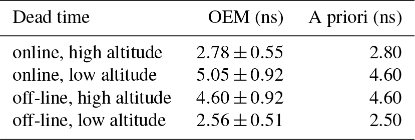
For the two wavelengths and two different altitude channels, the dead time can differ. Therefore, we are retrieving the dead times for each altitude and at each wavelength. A dead time value that corresponds to the x parameter of each channel at each night is used as our a priori, and an uncertainty of ±20 % is assigned to it.
Using the OEM, we retrieve the ozone density and air density profiles, as well as the dead time values for the four channels, the background counts for the off-line channel, and the SIN coefficients (three values) for the online channel. In total, we retrieved eight quantities along with the ozone density and air density profiles. The degree of freedom for our measurements, which is the trace of the averaging kernel, is ≈78. Below we present the ozone retrieval for 26 July 2017 in detail. In order to show that the OEM is a robust method, results for the nights of 14 and 20 July are presented as well. On all these nights, ozonesonde balloons were coincidentally launched, and thus the OEM is validated against both the traditional method and the sonde measurements.
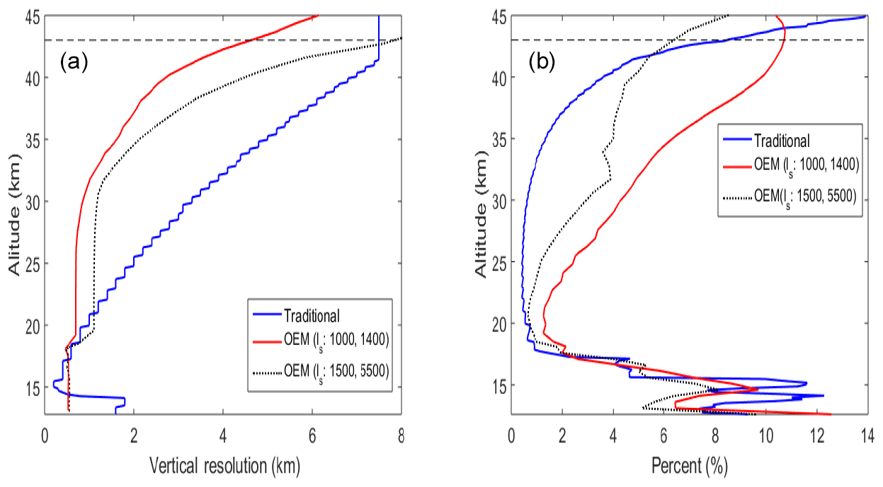
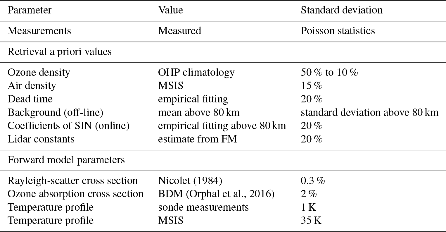
Figure 5(a) The vertical resolution of the OEM with correlation lengths ℓs = 1000 and 1400 m (red curve) is plotted against the vertical resolution of the OEM with correlation lengths ℓs = 1400 and 5500 m (black dotted curve). The vertical resolution of the traditional method is shown as well (blue curve). (b) The statistical uncertainty of the OEM with correlation lengths ℓs = 1000 and 1400 m is plotted (red curve) against the statistical uncertainty of the OEM with correlation lengths ℓs = 1400 and 5500 m (black dotted curve). Additionally, the uncertainty of retrieval in the traditional method (blue curve) is plotted. The retrieval uncertainties in the OEM and the traditional method can be compared. The horizontal dashed line is a height below which the OEM retrieval is more than 80 % due to the measurements.
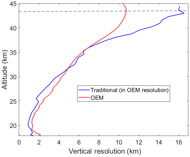
Figure 6At a height from 20 to 40 km, the uncertainty of retrieval for the traditional method (assuming that it has a vertical resolution similar to the OEM vertical resolution) is plotted against the OEM retrieval uncertainty (blue curve: OEM; red curve: traditional).
4.1 Applying the OEM to OHP measurements on 26 July 2017
Figure 2 shows the averaged counts over 4 h of measurements for two different channels at online and off-line wavelengths on the night of 26 July 2017. The coincident ozonesonde is launched within 1 h after the start of the measurement and takes approximately 2 h to reach 30 km. For each retrieval, the averaging kernel matrix is calculated. The averaging kernel is a diagnostic variable that describes how the retrieval sees changes in the real atmosphere. Therefore, it contains information on the sensitivity (area of the averaging kernel function) and on the smoothing (shape of the averaging kernel function) of the retrievals. Ideally the averaging kernel is a unity matrix preserving any change in the retrieved quantity from the a priori state. The area is defined as the vector product Au, where u is a unit vector. When the retrieval comes solely from the measurements, then the area equals 1, and at altitudes at which the a priori profile is contributing to the retrievals the area decreases; an area equal to 0 would mean nothing is being retrieved.
Figure 3 shows the averaging kernels for the ozone density. The dashed line shows that the averaging kernel for ozone density equals 1 up to 42.7 km, and thus below this altitude the retrieval is independent of the a priori profile. Ozone is a minor constituent in the atmosphere; due to the poor SNR of signals at higher altitudes, the sensitivity of the averaging kernel decreases. Here, the retrieval falls back to the a priori values.
Figure 7The traditional statistical uncertainty (blue curve) is plotted when the retrieval has the same vertical resolution as the OEM; the statistical uncertainty of the OEM is plotted in red.
In a good retrieval, the difference between the forward model and the measurements, which is called the residual, should be within the uncertainty of the measurements. Figure 4 shows the residual plots, which confirm that our forward model has correctly characterized the physics of the atmosphere and is capable of retrieving the quantity of interest.
The OEM retrieval grid starts at 500 m and increases to 700 m at 18 km. The full width half maximum of the averaging kernel at each height is defined as the vertical resolution of the retrieval. At lower altitudes, the averaging kernel is broad, and the retrieval resolution is close to the spacing of the retrieval grid (for this specific retrieval around 500 m). As shown in Fig. 5b, by increasing the altitude, the retrieval resolution consequently decreases such that at 40 km the resolution is 2.8 km. Traditionally, the vertical resolution decreased by height as well. Figure 5a shows the vertical resolution of the retrieval in both traditional methods and the OEM. At the first 2 km of retrieval the OEM provides a better retrieval resolution; however, from 14.5 to 17 km the traditional method has a better resolution. At around 17 km both methods show the same retrieval resolution; however, the traditional resolution decreases faster such that at 42.2 km the retrieval resolution is around 7 km. The trade-off between the retrieval resolution and the retrieval uncertainty should be considered when comparing the methods, and the reader is referred to the discussion below.
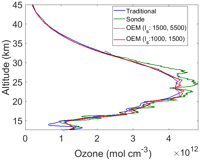
Figure 8OEM ozone retrieval (red curve) from 20:07 to 00:15 UT on 26 July 2017 as well as the ozonesonde profile (green curve) and the traditional ozone retrieval (blue curve) are plotted. The dashed black line shows the OEM retrieval when the correlation length (łS) became larger. The horizontal dashed line shows the cutoff below which the effect of the a priori ozone profile is small (less than 10 %).
Table 2Dead time values that were calculated for each channel on the night of 26 July 2017.
Having a poorer vertical resolution leads to a better (that is, smaller) retrieval uncertainty. As shown in Fig. 5b, the statistical uncertainty of the retrievals for the traditional method is around 12 % at 15 km (when the vertical resolution is 200 m and the low-altitude Rayleigh channel is used) and it decreases to less than 1 % at 25 km (when the vertical resolution is around 2 km and the high-altitude Rayleigh channel is used). In contrast, the statistical uncertainty of retrieval in the OEM is around 10 % at 15 km (when the vertical resolution is 500 m) and decreases to 2.2 % at 25 km (when the vertical resolution is 700 m).
To demonstrate the mentioned trade-off in the OEM, we increased the correlation length of the a priori from 1000 to 1500 m in the lower altitudes (below 18 km) and from 1400 to 5500 m in higher altitudes (above 18 km). As a result, the retrieval has a poorer vertical resolution and smaller retrieval uncertainties. Assuming a higher correlation length indicates that at each altitude, the retrieved ozone density is dependent on the ozone distribution above and below the indicated altitude; thus, the retrieved ozone density looks smoother.
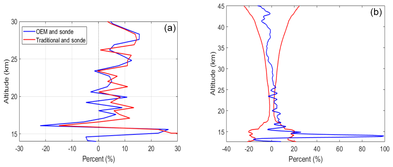
Figure 9For the night of 26 July 2017. (a) The percentage difference between the OEM retrieval and the ozonesonde measurements in the form of (blue curve); the percentage difference between the traditional retrieval and the ozonesonde measurements in the form of (red curve). The difference between the traditional method, as the sonde profile below 14 km is greater than 100 %, is thus not shown in the figure. (b) The percentage difference between the OEM retrieval and the traditional retrieval (blue curve); the summation of the statistical uncertainty of the traditional and OEM retrievals (red curve).
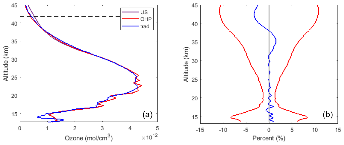
Figure 10For the night of 26 July 2017. (a) the OEM retrieval using the US standard model as an a priori profile (purple curve) and the OEM retrieval using the OHP climatology as an a priori profile (red curve) are plotted. Furthermore, the traditional method retrieval (blue curve) is plotted, and thus the OEM retrievals can be compared with each other and with the traditional retrieval. (b) Percentage difference between the OEM retrievals using the two different a priori profiles (blue curve) is plotted. This difference is within the retrieval uncertainty. At higher altitudes (above 35 km) when the SNR drops, the difference between the two methods is less than 5 %, which is smaller than the retrieval uncertainty at that height.
The vertical resolution and uncertainty for the traditional method as well as for the OEM with low and high correlation lengths are plotted in Fig. 5.
In the traditional method, the relation between the final vertical resolution and the retrieval uncertainty is defined as follows:
where ϵs is the retrieval uncertainty, A is the area of the telescope, Δzf is the final vertical resolution, P0 is the emitted power, and ta is the acquisition time (Godin et al., 1999). Assuming that the traditional method has the same vertical resolution as the OEM, using the above relation we can calculate the retrieval uncertainty, which corresponds to the higher vertical resolution. Despite the difference in the vertical resolution values, at altitudes below 20 km, both the traditional method and the OEM have similar uncertainties (the difference is less than 1 %). At altitudes above 20 km, assuming that the traditional method has the same vertical resolution as OEM, the retrieval uncertainty in the traditional method is calculated. Figure 6 shows the comparison between OEM uncertainty and the modified traditional uncertainty for altitudes above 20 km. From 20 to 35 km the difference between the uncertainties is insignificant (less than 1 %), while above 35 km the difference grows to 4.5 %.
The traditional ozone profile can be calculated at a similar vertical resolution to our OEM retrieval. The statistical uncertainty of the traditional analysis, using the same vertical resolution as our OEM, is shown in Fig. 7. Below 30 km both methods provide the same uncertainties; however, above this altitude the OEM uncertainty is smaller. The OEM's smaller statistical uncertainty at higher altitudes increases more slowly than for the traditional method due to the contribution of the a priori profile, which adds additional information. However, in the OEM retrieval an increased contribution from the regularization term of the solution means the response function becomes less than 1. Below 30 km the a priori profile has a small contribution to the final retrieval (as the response function is ∼1), but between 30 and 40 km the a priori profile has a greater contribution. Above 40 km the response function decreases rapidly (Fig. 3).
Figure 8 shows our retrieved ozone density compared to the sonde measurements and the traditional retrieval. Consistent with Fig. 5 we have plotted the OEM retrievals for two different sets of correlation lengths. The ozonesonde measurements have better vertical resolutions compared to the DIAL measurements, albeit with larger random uncertainty. Also, the sonde profiles show more vertical structure of the ozone distribution. Compared to the traditional retrieval, the OEM can successfully catch many of these variations.
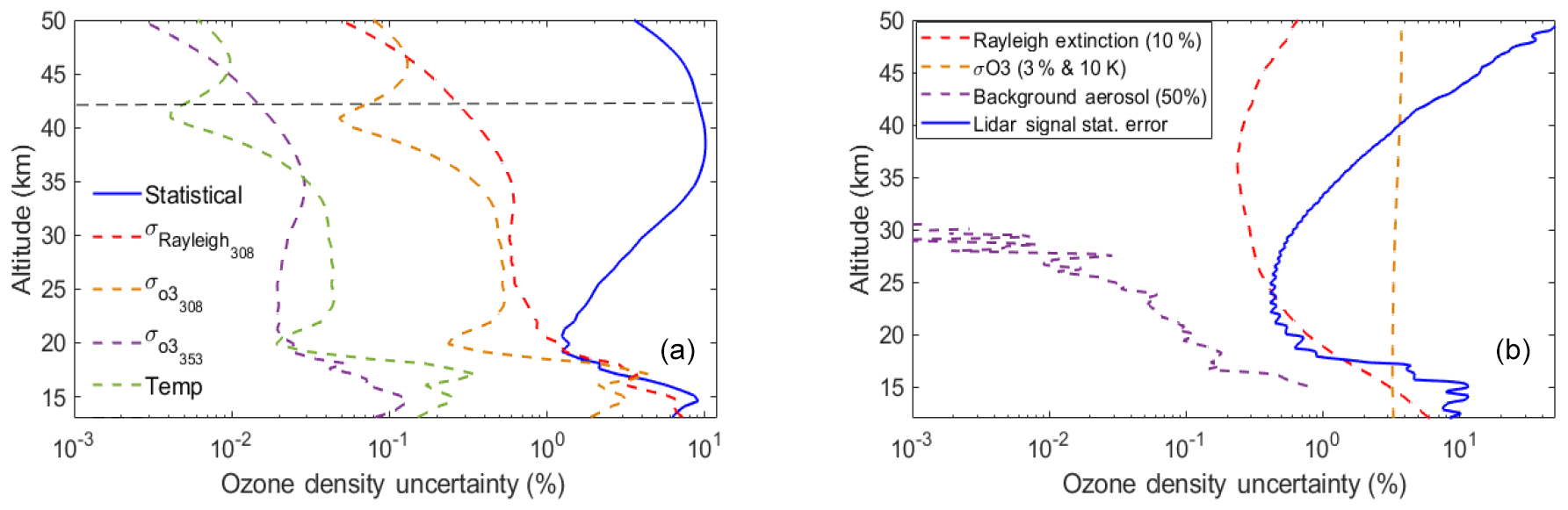
Figure 11For the night of 26 July 2017. The statistical uncertainty of the OEM (blue), the Rayleigh-scatter cross section uncertainty at 308 nm (red), the ozone absorption cross section at 308 nm (orange), and the ozone absorption cross section for the 355 nm channel (purple). The horizontal dashed line shows the height below which the retrieval is independent of the a priori profile.
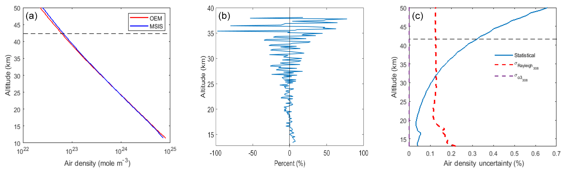
Figure 12(a) The retrieved air density (blue line) is plotted against the a priori profile (red line). (b) The percentage difference between the scaled relative air density generated from the Raman channel and the OEM air density retrievals. The difference is less than 10 %. (c) The statistical uncertainty of the OEM retrieval of air density (blue), the Rayleigh-scatter cross section uncertainty for the 308 nm channel (red), and the ozone absorption cross section in both channels (purple).
In order to account for the higher vertical resolution of the ozonesonde measurements, we use the OEM averaging kernels to “degrade” (smooth) the sonde profile using
where In is the unity matrix, and xsmoothed is the smoothed sonde profile. Figure 9a shows the percentage difference between the smoothed sonde and the OEM (in blue) as well as the percentage difference between the smoothed sonde and the traditional profile (in red). The difference between the sonde and the traditional analysis at 14 km is greater than 100 %. Figure 9b shows a comparison between the two lidar methods. For higher altitudes (above 25 km) the difference between the two retrievals is less than the statistical uncertainty of the measurement. However, for lower altitudes (between 14 and 21 km) the difference between the two methods is significant.
To investigate the effect of a priori profiles on retrievals, the OHP climatology and the US standard model were used to retrieve ozone density (see Fig. 10). The OEM retrievals resulting from these two a priori profiles as well as the traditional retrieval are plotted in Fig. 10a. As shown in the panel (b) of this figure, below 35 km the difference between the two OEM retrievals is less than 0.5 %. Above this altitude, the percentage difference between the two methods reaches 2.5 %, which is much smaller than the retrieval uncertainty at altitudes above 35 km. Thus, the choice of a priori has a small effect on the retrievals.
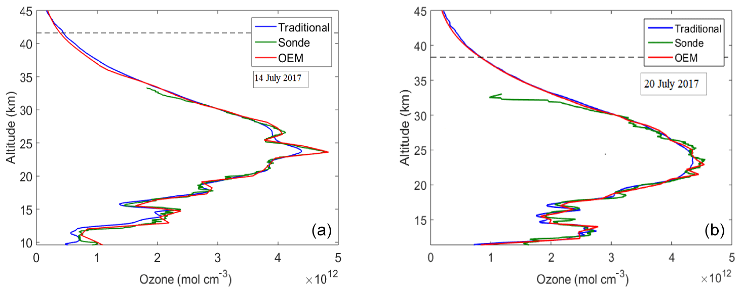
Figure 13(a) OEM ozone retrieval on the night of 14 July 2017 (red curve) compared to the ozonesonde profile (green curve) and the traditional ozone retrieval (blue curve). (b) OEM ozone retrieval on the night of 20 July 2017 (red curve) compared to the ozonesonde profile (green curve) and the traditional ozone retrieval (blue curve). These cases demonstrate the high resolution of the OEM technique as evidenced by the excellent agreement around the ozone peak with the sonde measurement.

Figure 14For the night of 14 July 2017, (a) the percentage difference between the traditional method and the OEM retrieval (blue curve) plotted within the envelope of the total statistical uncertainty of the two methods (red curve). The agreement between the two lidar ozone determinations is within the statistical uncertainty above 17 km. (b) The red curve is the percentage difference between the OEM retrieval and sonde measurements. The blue curve is the percentage difference between the traditional method and sonde measurements. Panels (c) and (d) are the same format as (a) and (b) for the night of 20 July 2017.
The OEM provides a complete systematic and statistical uncertainty budget. Figure 11a shows the uncertainty of the OEM ozone retrieval shown in Fig. 8. The forward model parameters, the Rayleigh cross sections, the ozone absorption cross section, and the temperature profiles assumed for the ozone cross section contribute to the systematic uncertainty of the retrieval. Below 20 km, these uncertainties are comparable with the statistical uncertainty; however, in the higher altitudes systematic uncertainties are less than 1 %. The Rayleigh-scatter cross section uncertainty, at the bottom of the retrieval, is around 7 %, while at higher altitudes the uncertainty decreases to less than 1 %. These values agree with the Rayleigh-scatter uncertainty of 8 %, which is calculated in the Leblanc et al. (2016b) uncertainty budget. The ozone absorption cross section for the 308 nm channel reached a maximum of 4 % at the bottom of the retrieval, which is higher than the calculated uncertainty of 1 % in Leblanc et al. (2016b). The uncertainty due to temperature is less than 0.05 %. The uncertainty due to the ozone absorption cross section at the 355 nm channel is negligible as well.
The calculated OEM uncertainty can be compared with the traditional uncertainty budget. Figure 11b shows the uncertainty of the traditional ozone profile. The Rayleigh-scatter cross section uncertainty has a maximum value of 8 % at the bottom of the profile, while above 20 km it becomes less than 1 %. This result is consistent with the uncertainty calculated by our OEM retrieval. In the traditional analysis, for an isothermal atmosphere, the ozone absorption cross section uncertainty at 308 nm is 3 %. The ozone absorption cross section uncertainty in our OEM retrieval is similar to Leblanc et al. (2016b), whose Monte Carlo simulations allowed temperature to vary with height. In the traditional analysis, the background aerosol uncertainty is also calculated, which impacts the ozone profile by less than 1 % in the lower stratosphere. Aerosols are currently being added to the OEM forward model as a model parameter. The statistical uncertainty of the traditional analysis at higher altitudes (above 25 km) is smaller compared to the OEM, which as explained earlier is the result of having a larger vertical resolution. However, as shown in Fig. 5 (the black dotted lines), the OEM retrievals also have smaller statistical uncertainties if the vertical resolution increases. As discussed previously (Fig. 6), for the traditional analysis using a similar vertical resolution to our OEM, the statistical uncertainty of the traditional method will be larger than for the OEM retrievals in the upper stratosphere due to the regularization term in the OEM.
The acceptable range of ozone retrieval extends from 12 to 42.7 km. The averaging kernel of the air density extends much higher, as the air density contributes to both backscattering coefficients and the extinction coefficient terms in the forward model. Therefore, in air density retrievals, the maximum height of acceptable retrieval is 70.2 km. However, we show the retrievals below 42.7 km to be consistent with the ozone density retrievals. As shown in Fig. 12a, the relative air density profile is retrieved as well.
To validate our result, we used the nitrogen Raman spectrum at 386.7 nm. The off-line wavelength is transmitted to the atmosphere at the 355 nm channel, and the corresponding Raman wavelength is received at the 386.7 nm channel. The Raman channel is not sensitive to the aerosol contents of the atmosphere, and the wavelength is not absorbed by ozone (off-line Raman channel). Thus, the atmospheric backscattering and extinction terms are mostly determined by the air density. This makes the Raman off-line channel a good candidate for our validation. We can assume that .
Using the above relation, the relative air density profile can be generated. The relative air density is scaled against the OEM retrieval of air density, and the percentage difference is calculated (Fig. 12b).
As shown in the figure, the difference between the scaled relative air density generated from the Raman counts and the OEM relative air density is less than 10 %. However, in higher altitudes (above 35 km) the difference can reach up to 50 %. This difference is governed by the higher measurement noise in the Raman channel. This result provides confidence that the density retrieval is reasonable. Figure 12c shows the uncertainty of the relative air density retrieval. For the air density retrieval the statistical uncertainty is small (around 0.1 % at the bottom of the retrieval). The Rayleigh-scatter cross section uncertainty is small as well, and the ozone absorption cross section uncertainties are negligible.
The OHP analysis employing the traditional method uses a different value of saturation correction for each wavelength. In our OEM code, we are retrieving four different dead times, each corresponding to one of the channels. For a priori values, we are using the provided x value, which is discussed earlier in this section. As shown in Table 2, the retrieved dead time values for 26 July 2017 are similar to the provided x values. The only major difference is detected for the online low-altitude channel, for which the x value is 4.6 ns and the retrieved value is 5.05 ns.
4.2 Further examples of the OEM retrieval method
The ozone profiles retrieved using our OEM for the nights of 14 and 20 July, the coincident sonde measurements, and the traditional ozone retrievals are shown in Fig. 13. The night of 14 July 2017 includes 4.5 h of measurements. The retrieval extends from 9.6 to 40.2 km. Above 16 km, the difference between the two traditional methods and the OEM retrieval is within the statistical uncertainty of the measurements. Between 16 and 19 km the difference between the OEM and the sonde becomes large; this is coincidental with the two peaks measured by the sonde at these two altitudes (see Fig. 13). After smoothing (degrading) the sonde profiles the two picks are much smoother, and this causes the large difference between the OEM and sonde profiles (Fig. 14). For 20 July 2017 the retrieval is computed using 4 h of measurements. The ozone retrieval extends from 11 to 36.8 km. The differences between the two methods are within the retrieval uncertainty (Fig. 14). For both nights the difference between the sonde and the calculated profiles below 13.5 km is larger than 80 % and is thus not shown here. These two additional nights help to demonstrate that the OEM can produce high-quality ozone density profiles that are consistent with the traditional profiles found using the traditional method.
We have introduced a first-principle OEM retrieval for stratospheric ozone profiles applicable to stratospheric DIAL measurements and tested this method using measurements from the OHP stratospheric DIAL system. The discussion of the implementation of OEM for our retrievals is summarized below.
-
The forward model used in this study is capable of providing a robust estimate of ozone profiles for clear nights.
-
Multiple measurements channels are used. The raw (uncorrected) photocounts are used for the retrieval, and no gluing process is needed. As a result, a single ozone profile consistent with all measurements is retrieved.
-
The OEM is applied to the OHP lidar measurements for three different nights in July 2017, all of which had coincident ozonesonde launches. Comparison with the radiosondes was good.
-
The OEM's averaging kernels allow the contribution of the a priori relative to the measurements to be accessed as a function of altitude, as well as allowing better comparison with other instruments.
-
The OEM and the traditional method show good agreement, and for most heights their difference is small.
-
Increasing the correlation length in the retrieval allows the vertical resolution to be degraded and the statistical uncertainty decreased. Comparisons with the OEM retrievals at degraded resolution showed agreement with the traditional method to within the statistical uncertainty of the measurements.
-
The OEM provides a full uncertainty budget. Thus, using the OEM, for each individual retrieved profile both statistical and systematic uncertainties are calculated. The systematic uncertainties are compared with the uncertainty budget for the traditional method given by Leblanc et al. (2016a) and are similar.
Currently we are working on a retrieval that can use measurements from both the OHP tropospheric and stratospheric lidars, which will allow us to retrieve ozone profiles from just above the boundary layer throughout the stratosphere. Also, we plan to include the Raman measurements in our forward model, allowing for the retrieval of ozone profiles in the presence of strong aerosol layers and thin clouds. We are planning to apply our OEM retrieval to the last 3 decades of OHP measurements. Applying the OEM to the entire OHP lidar ozone profile database will provide an improved statistical evaluation of the differences between traditional and OEM methods, as well as allowing for improved ozone estimates in the upper troposphere and lower stratospheric region.
The data used in this paper are available at ftp://ftp.cpc.ncep.noaa.gov/ndacc/station/ohp/ (last access: last access: 7 March 2019).
GF was responsible for developing the DIAL OEM routine as well as for proving the comparisons between the OEM and traditional methods. She also wrote the initial draft of the paper. RJS was GF's PhD supervisor. He defined the project and participated in the development of the OEM code. SGB provided the lidar measurements and performed the traditional analysis of the measurements. AH participated in the definition of the project and the implementation of the DIAL OEM code.
The authors declare that they have no conflict of interest.
We would like to thank Tom McElroy and Shayamila Mahagammulla Gamage for many interesting discussions about OEM, Tom in particular for recognizing the potential of using OEM for lidar retrievals. We would like to thank Google Engine, which selflessly helped us browse the world. We greatly appreciate the editing help from Patricia Sica, who patiently proofread an earlier version of the paper. This project has been funded in part by the National Science and Engineering Research Council of Canada. The OHP lidar systems are funded by the National Center for Scientific Research. We would also like to thank the lidar operators of the station Gèrard Mègie at Haute-Provence Observatory.
This paper was edited by Frank Hase and reviewed by two anonymous referees.
Andrews, D. G., Holton, J. R., and Leovy, C. B.: Middle atmosphere dynamics, 40, Academic press, London, UK, 1987. a
Ball, W. T., Alsing, J., Mortlock, D. J., Staehelin, J., Haigh, J. D., Peter, T., Tummon, F., Stübi, R., Stenke, A., Anderson, J., Bourassa, A., Davis, S. M., Degenstein, D., Frith, S., Froidevaux, L., Roth, C., Sofieva, V., Wang, R., Wild, J., Yu, P., Ziemke, J. R., and Rozanov, E. V.: Evidence for a continuous decline in lower stratospheric ozone offsetting ozone layer recovery, Atmos. Chem. Phys., 18, 1379–1394, https://doi.org/10.5194/acp-18-1379-2018, 2018. a
Donovan, D. P., Bird, J. C., Whiteway, J. A., Duck, T. J., Pal, S. R., and Carswell, A. I.: Lidar observations of stratospheric ozone and aerosol above the Canadian high arctic during the 1994–95 winter, Geophys. Res. Lett., 22, 3489–3492, 1995. a
Eriksson, P., Jimenez, C., and Buehler, S.: Qpack, a general tool for instrument simulation and retrieval work, J. Quant. Spectrosc. Ra., 91, 47–64, 2005. a, b
Farman, J. C., Gardiner, B. G., and Shanklin, J. D.: Large losses of total ozone in Antarctica reveal seasonal ClOx∕NOx interaction, Nature, 315, 207, 1985. a
Fernald, F. G.: Analysis of atmospheric lidar observations: some comments, Appl. Optics, 23, 652–653, 1984. a
Godin, S., Carswell, A. I., Donovan, D. P., Claude, H., Steinbrecht, W., McDermid, I. S., McGee, T. J., Gross, M. R., Nakane, H., Daan, Swart, P. J., Bergwerff, B. B., Uchino, O., von der Gathen, P., and Neuber, R.: Ozone differential absorption lidar algorithm intercomparison, Appl. Optics, 38, 6225–6236, 1999. a, b, c
Godin-Beekmann, S., Porteneuve, J., and Garnier, A.: Systematic DIAL lidar monitoring of the stratospheric ozone vertical distribution at Observatoire de Haute-Provence (43.92∘ N, 5.71∘ E), J. Environ. Monitor., 5, 57–67, 2003. a, b, c, d
Harris, N. R. P., Hassler, B., Tummon, F., Bodeker, G. E., Hubert, D., Petropavlovskikh, I., Steinbrecht, W., Anderson, J., Bhartia, P. K., Boone, C. D., Bourassa, A., Davis, S. M., Degenstein, D., Delcloo, A., Frith, S. M., Froidevaux, L., Godin-Beekmann, S., Jones, N., Kurylo, M. J., Kyrölä, E., Laine, M., Leblanc, S. T., Lambert, J.-C., Liley, B., Mahieu, E., Maycock, A., de Mazière, M., Parrish, A., Querel, R., Rosenlof, K. H., Roth, C., Sioris, C., Staehelin, J., Stolarski, R. S., Stübi, R., Tamminen, J., Vigouroux, C., Walker, K. A., Wang, H. J., Wild, J., and Zawodny, J. M.: Past changes in the vertical distribution of ozone – Part 3: Analysis and interpretation of trends, Atmos. Chem. Phys., 15, 9965–9982, https://doi.org/10.5194/acp-15-9965-2015, 2015. a, b
Heath, D. F., Schlesinger, B. M., and Park, H.: Spectral change in the ultraviolet absorption and scattering properties of the atmosphere associated with the eruption of El Chichón: Stratospheric SO2 budget and decay, Eos Trans. AGU, 64, 168–181, 1983. a
Hunt, W. H. and Poultney, S. K.: Testing the linearity of response of gated photomultipliers in wide dynamic range laser radar systems, IEEE T. Nucl. Sci., 22, 116–120, 1975. a
Iikura, Y., Sugimoto, N., Sasano, Y., and Shimzu, H.: Improvement on lidar data processing for stratospheric aerosol measurements, Appl. Optics, 26, 5299–5306, 1987. a, b
Krueger, A. J. and Minzner, R. A.: A mid-latitude ozone model for the 1976 US Standard Atmosphere, J. Geophys. Res.-Atmos., 81, 4477–4481, 1976. a
Leblanc, T., Sica, R. J., van Gijsel, J. A. E., Godin-Beekmann, S., Haefele, A., Trickl, T., Payen, G., and Gabarrot, F.: Proposed standardized definitions for vertical resolution and uncertainty in the NDACC lidar ozone and temperature algorithms –Part 1: Vertical resolution, Atmos. Meas. Tech., 9, 4029–4049, https://doi.org/10.5194/amt-9-4029-2016, 2016a. a, b, c
Leblanc, T., Sica, R. J., van Gijsel, J. A. E., Godin-Beekmann, S., Haefele, A., Trickl, T., Payen, G., and Liberti, G.: Proposed standardized definitions for vertical resolution and uncertainty in the NDACC lidar ozone and temperature algorithms – Part 2: Ozone DIAL uncertainty budget, Atmos. Meas. Tech., 9, 4051–4078, https://doi.org/10.5194/amt-9-4051-2016, 2016b. a, b, c, d, e
Malicet, J., Daumont, D., Charbonnier, J., Parisse, C., Chakir, A., and Brion, J.: Ozone UV spectroscopy. II. Absorption cross-sections and temperature dependence, J. Atmos. Chem., 21, 263–273, 1995. a
McDermid, I. S., Godin, S. M., and Walsh, D.: Lidar measurements of stratospheric ozone and intercomparisons and validation, Appl. Optics, 29, 4914–4923, 1990. a, b
Megie, G. J., Ancellet, G., and Pelon, J.: Lidar measurements of ozone vertical profiles, Appl. Optics, 24, 3454–3463, 1985. a
Nicolet, M.: On the molecular scattering in the terrestrial atmosphere: An empirical formula for its calculation in the homosphere, Planet. Space Sci., 32, 1467–1468, 1984. a
Orphal, J., Staehelin, J., Tamminen, et al.: Absorption cross-sections of ozone in the ultraviolet and visible spectral regions: Status report 2015, J. Mol. Spectrosc., 327, 105–121, 2016. a
Pelon, J. and Mégie, G.: Ozone monitoring in the troposphere and lower stratosphere: Evaluation and operation of a ground-based lidar station, J. Geophys. Res.-Oceans, 87, 4947–4955, 1982. a
Povey, A. C., Grainger, R. G., Peters, D. M., and Agnew, J. L.: Retrieval of aerosol backscatter, extinction, and lidar ratio from Raman lidar with optimal estimation, Atmos. Meas. Tech., 7, 757–776, https://doi.org/10.5194/amt-7-757-2014, 2014. a
Rodgers, C. D.: Inverse methods for atmospheric sounding: theory and practice, vol. 2, World scientific, Singapore, 2000. a
Schotland, R.: Errors in the Lidar Measurement of Atmospheric Gases by Differential Absorption, J. Appl. Meteorol., 13, 71–77, https://doi.org/10.1175/1520-0450(1974)013<0071:EITLMO>2.0.CO;2, 1974. a
Sica, R. J. and Haefele, A.: Retrieval of temperature from a multiple-channel Rayleigh-scatter lidar using an optimal estimation method, Appl. Opt, 54, 1872–1889, 2015. a
Sica, R. J. and Haefele, A.: Retrieval of water vapor mixing ratio from a multiple channel Raman-scatter lidar using an optimal estimation method, Appl. Opt, 55, 763–777, 2016. a
Solomon, S., Ivy, D. J., Kinnison, D., Mills, M. J., Neely, R. R., and Schmidt, A.: Emergence of healing in the Antarctic ozone layer, Science, aae0061, 269–274, 2016. a
WMO: Scientific Assessment of Ozone Depletion: 2010 Global Ozone Research and Monitoring Project Report 52, World Meteorological Organization, Geneva, 2011. a
WMO: Scientific Assessment of Ozone Depletion: 2014 Global Ozone Research and Monitoring Project Report, World Meteorological Organization, Geneva, 2014. a, b, c