the Creative Commons Attribution 4.0 License.
the Creative Commons Attribution 4.0 License.
 | 10 Apr 2019
Intercomparison of MAX-DOAS vertical profile retrieval algorithms: studies using synthetic data
Udo Frieß
Steffen Beirle
Leonardo Alvarado Bonilla
Tim Bösch
Martina M. Friedrich
François Hendrick
Ankie Piters
Andreas Richter
Michel van Roozendael
Vladimir V. Rozanov
Elena Spinei
Jan-Lukas Tirpitz
Tim Vlemmix
Thomas Wagner
Yang Wang
Multi-axis differential optical absorption spectroscopy (MAX-DOAS) is a widely used measurement technique for the detection of a variety of atmospheric trace gases. Using inverse modelling, the observation of trace gas column densities along different lines of sight enables the retrieval of aerosol and trace gas vertical profiles in the atmospheric boundary layer using appropriate retrieval algorithms. In this study, the ability of eight profile retrieval algorithms to reconstruct vertical profiles is assessed on the basis of synthetic measurements. Five of the algorithms are based on the optimal estimation method, two on parametrised approaches, and one using an analytical approach without involving any radiative transfer modelling. The synthetic measurements consist of the median of simulated slant column densities of O4 at 360 and 477 nm, as well as of HCHO at 343 nm and NO2 at 477 nm, from seven datasets simulated by five different radiative transfer models. Simulations are performed for a combination of 10 trace gas and 11 aerosol profiles, as well as 11 elevation angles, three solar zenith, and three relative azimuth angles. Overall, the results from the different algorithms show moderate to good performance for the retrieval of vertical profiles, surface concentrations, and total columns. Except for some outliers, the root-mean-square difference between the true and retrieved state ranges between (0.05–0.1) km−1 for aerosol extinction and (2.5–5.0) ×1010 molec cm−3 for HCHO and NO2 concentrations.
- Article
(19620 KB) -
Supplement
(6470 KB) - BibTeX
- EndNote


The planetary boundary layer (PBL) is the part of the atmosphere that is in direct contact with the terrestrial biosphere. Its chemical composition is determined by anthropogenic and natural emissions. Monitoring of both chemical composition and aerosol content of the PBL is crucial for the understanding of the chemical and physical processes and the spatio-temporal evolution of PBL composition. A versatile tool for the monitoring of atmospheric trace gases and aerosol content of the PBL is the well-known multi-axis differential optical absorption spectroscopy (MAX-DOAS) (e.g. Hönninger et al., 2004; Wagner et al., 2004; Heckel et al., 2005; Frieß et al., 2006; Platt and Stutz, 2008; Irie et al., 2008; Clémer et al., 2010; Wagner et al., 2011; Vlemmix et al., 2015b). It relies on the spectral analysis of scattered sunlight and enables the simultaneous detection of numerous trace gases, such as nitrogen dioxide (NO2), formaldehyde (HCHO), nitrous acid (HONO), water vapour (H2O), sulfur dioxide (SO2), ozone (O3), and halogen oxides. Measurements along different lines of sight, with elevation angles (EAs) ranging from near the horizon to the zenith, allow for the reconstruction of vertical profiles of the measured trace gases and, using the oxygen collision complex O4 as a proxy for the light path, also of aerosol extinction. Using suitable inverse models, trace gas and aerosol profiles can be retrieved in the lowermost ≈2 km with a vertical resolution of about 50–100 m at the surface and a lower resolution above. Up to four independent pieces of information can be retrieved.
Algorithms for the retrieval of vertical profiles from MAX-DOAS measurements can be separated into those that retrieve vertical profiles on a finite vertical grid (usually with layers of 50–200 m in thickness) using the optimal estimation method (OEM) (Rodgers, 2000) and parametrised algorithms that use a small number of parameters (typically two to four) to describe the shape of the atmospheric profile. Parametrised algorithms are typically faster than OEM algorithms since they are usually based on precalculated look-up tables (LUTs), while OEM algorithms rely on online radiative transfer modelling (RTM). Being based on Bayesian statistics, OEM algorithms have the advantage of providing a thorough error analysis as well as a quantitative characterisation of the vertical resolution and the information content (Rodgers, 2000). However, the results of OEM algorithms critically depend on the appropriate choice of a priori constraints, which are in many cases difficult to assess. In addition to OEM and parametrised approaches, the present study also includes a fast algorithm developed by NASA, which relies only on geometrical considerations and only invokes radiative transfer modelling for a pure Rayleigh atmosphere.
Testing the performance of algorithms for the retrieval of the atmospheric state using remote-sensing measurements on the basis of synthetic data is a method that has been widely used in the scientific community. In particular, numerous synthetic studies that investigated the performance of MAX-DOAS retrieval algorithms were published in the past (Wagner et al., 2004; Frieß et al., 2006; Hay, 2010; Vlemmix et al., 2011; Yilmaz, 2012; Hartl and Wenig, 2013; Holla, 2013; Zielcke, 2015). This paper presents the first intercomparison of eight state-of-the-art algorithms for the retrieval of vertical profiles of aerosols and trace gases using synthetic MAX-DOAS measurements. Synthetic measurements have the advantage over ambient measurements that the true atmospheric state is exactly known, and thus a quantitative comparison of true and retrieved atmospheric states is straightforward. This study is part of the Fiducial Reference Measurements for Ground-Based DOAS Air-Quality Observations (FRM4DOAS) project funded by the European Space Agency (see http://frm4doas.aeronomie.be, last access: 8 April 2019). One of the main objectives of this project is the development of a community algorithm for a harmonised near-real-time processing of MAX-DOAS data, including spectral analysis as well as the retrieval of tropospheric profiles of aerosols, HCHO and NO2, and stratospheric NO2 profiles as well as total ozone columns. As part of the FRM4DOAS project, the aim of the study presented here has been the selection of suitable algorithms for the retrieval of tropospheric profiles to be integrated in the FRM4DOAS community algorithm.
The paper is structured as follows: Sect. 2 briefly describes the inverse modelling theory and outlines the strategy for the intercomparison of the profile retrieval algorithms. A short description of the individual retrieval algorithms is provided in Sect. 3. The model scenarios and RTM settings are specified in Sect. 4. Slant column densities (SCDs) of NO2, HCHO, and the oxygen collision complex O4, simulated by the different RTMs serving as forward models for the retrieval algorithms, are compared in Sect. 5. Comparisons of the quantities derived by the participating retrieval algorithms are presented in Sect. 6. These include averaging kernels from the OEM algorithms (Sect. 6.2), a posteriori modelled dSCDs (Sect. 6.3), vertical profiles (Sect. 6.4), total columns (Sect. 6.5), and aerosol extinctions and trace gas concentrations near the surface (Sect. 6.6). Finally, the numerical performance of the individual retrieval algorithms is assessed in Sect. 6.7.
In general, the retrieval of the atmospheric state (or the state of any physical system) by remote sensing is based on the observation of a finite number of quantities that represent the components of the measurement vector y, which is a function of the atmospheric state x,
Here, ϵ represents the measurement error. In the case of MAX-DOAS retrievals, the state vector x consists of either aerosol extinction coefficients or trace gas concentrations in discrete atmospheric layers with a typical thickness of 50–200 m. The measured quantities are differential slant column densities (dSCDs) dS, usually the difference between the SCD S at a certain EA α and the SCD from a zenith sky measurement, observed along different lines of sight:
with the SCD S being the integrated concentration along the (average) light path through the atmosphere.
Here, ρ is the number density of the trace gas and s parametrises the light path length through the atmosphere. The vector b in Eq. (1) represents additional forward model parameters, which are not to be retrieved, such as atmospheric pressure, temperature, aerosol optical properties, etc. The aim of an inverse model is to provide an estimate of the atmospheric state x for a given measurement y. However, inverse problems are often poorly constrained, and the inverse of the forward model function F−1, for which either does not exist or the finite measurement error ϵ leads to unstable estimates of the state vector.
To overcome these problems, MAX-DOAS retrieval algorithms make use of two different approaches. Retrieval algorithms using the well-known optimal estimation method (OEM) are based on a Bayesian approach (Rodgers, 2000). They introduce an a priori state vector xa, together with an a priori covariance matrix Sa, as an additional constraint. OEM algorithms are based on the minimisation of the following cost function:
Here Sϵ is the measurement covariance matrix, which, under the assumption that the measurements are independent, is a matrix with the squares of the measurement errors (specified in Sect. 6.1 and Table 6) as diagonal elements and zero values elsewhere. The most probable (maximum a posteriori, MAP) estimate is then given as
Table 1MAX-DOAS retrieval algorithms participating in this study
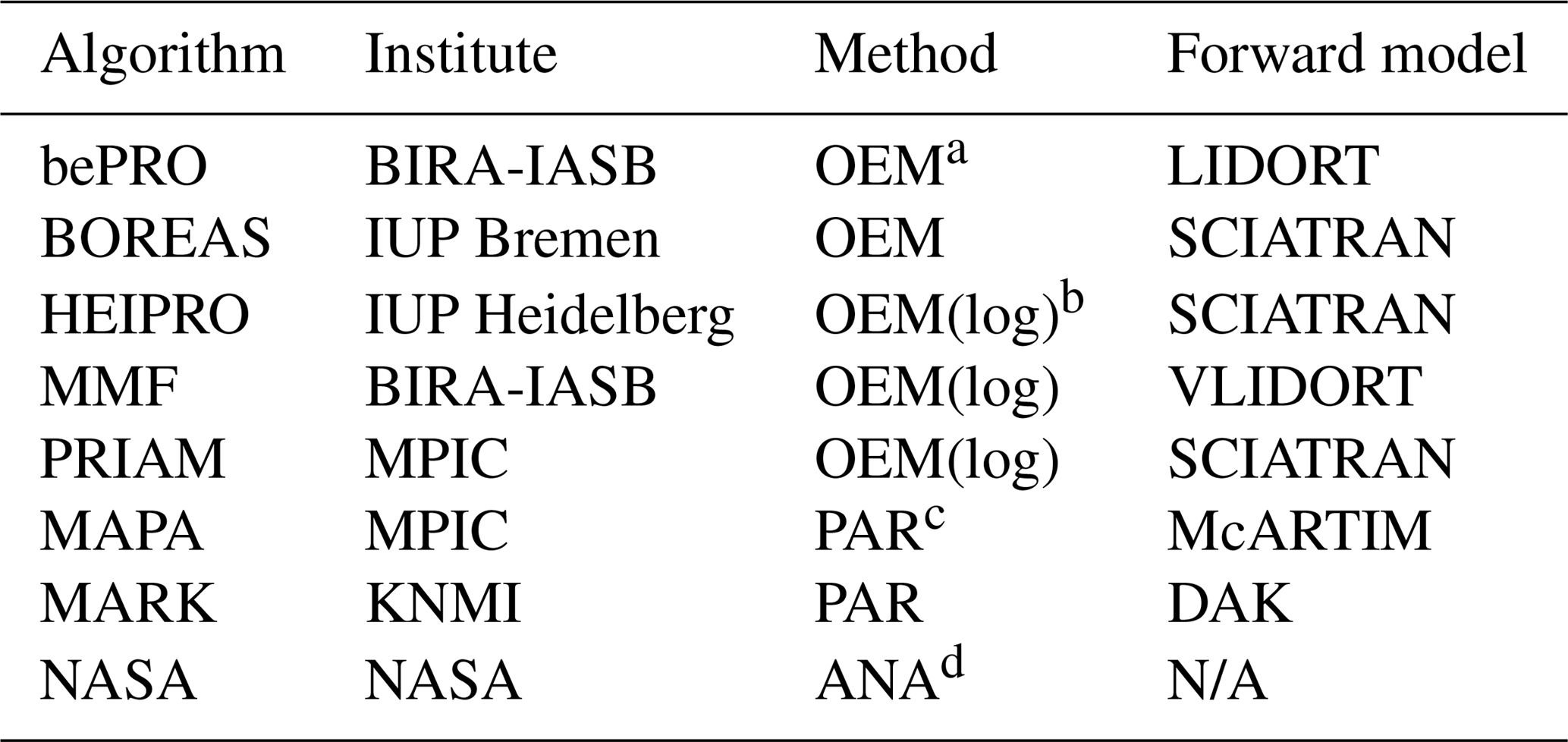
a Optimal estimation. b OEM(log): optimal estimation with logarithmic state vector. c Parametrised retrieval. d Analytical retrieval with RTM only for Rayleigh atmosphere.
The a priori constraints xa and Sa represent the best knowledge of the atmospheric state before the measurement has been made, which can be derived, for example, from climatologies, but are often only based on rough estimates of the typical atmospheric conditions at the measurement site. The averaging kernel matrix (AVK) A quantifies the sensitivity of the retrieved state to the true atmospheric state:
The degrees of freedom for signal (DFS) ds=Tr(A) quantify the number of independent pieces of information contained in the measurements. The jth row of the AVK represents the sensitivity of the retrieved amount in the atmospheric layer j to the amount in all other layers, and the retrieved profile can be expressed by the true atmospheric profile, smoothed by the AVK according to
Parametrised retrieval algorithms do not explicitly introduce a priori constraints but overcome the problem that the state vector is poorly constrained by the measurements by representing the state vector as x=x(p), using only a small number (typically two to four) of parameters that describe quantities such as the total column, the layer thickness, and the shape of the profile. The cost function of parametrised algorithms is given as
and the best estimate of the parameters is given as
OEM algorithms have the advantages that the approach, based on the well-established Bayesian statistics, is mathematically stringent and that important parameters, such as the retrieval covariance matrix (separated into smoothing and noise covariance), AVK, and information content, can be readily derived. Parametrised algorithms are usually faster than OEM algorithms since the small number of parameters allows for the usage of precalculated LUTs, whereas OEM algorithms, with a larger number of state vector elements, usually perform radiative transfer calculations online. The calculation of the Jacobian matrix (weighting function), which is required by OEM algorithms for the minimisation of the cost function, can be quite time consuming, especially for non-linear problems, such as the aerosol profile retrieval. Parametrised algorithms have the disadvantage that the parametrisation limits the possible representations of the state vector to a certain subspace of the state vector space when characterising the state vector with a limited number of parameters. Conversely, OEM algorithms tend to be biased to the a priori, in particular in regions where the sensitivity to the atmospheric state is low.
The overall strategy for the comparison of aerosol and trace gas vertical profiles from MAX-DOAS measurements within this study is depicted in Fig. 1. It consists of the following steps.
-
The first step of the intercomparison exercise consists of a comparison of the forward models of the individual retrieval algorithms. Simulations of SCDs of HCHO, NO2 and O4 are performed for a variety of atmospheric scenarios and viewing geometries as described in Sect. 4. In the following, these prescribed scenarios are referred to as the true atmospheric state, which is represented by the atmospheric state vector x. This forward model intercomparison exercise allows for a quantitative comparison of the individual RTMs on which the inversions are based (see Sect. 5).
-
The medians of the ensemble of dSCDs of HCHO, NO2 and O4 from the different forward models derived from step 1 serve as a reference dataset that represents the measurement vectors for the different atmospheric scenarios. This dataset was distributed among the participants of this study and serves as input for the individual retrieval algorithms. This dataset is referred to below as the (synthetic) measurements y.
-
The comparison of profiles retrieved by each participant on the basis of the reference dataset with the true aerosol and trace gas profiles x allows for a quantitative assessment of the inverse models. The results of this intercomparison will be presented in Sect. 6.
-
Finally, a comparison of the numerical performance of the individual retrieval algorithms is performed (Sect. 6.7).

This section briefly describes the eight MAX-DOAS retrieval algorithms whose main features are listed in Table 1. Five of the algorithms are based on OEM, two on a parametrised approach, and one (NASA) on an analytical approach without radiative transfer modelling. Each of the participants is free to decide on criteria for flagging particular retrieval results as invalid as described in the following subsections. If not stated otherwise, the comparison of retrieved quantities within this study is based on all data, without considering the validity flags.
3.1 The bePRO algorithm
The Belgian Profile (bePRO) OEM inversion algorithm was developed at the Royal Belgian Institute for Space Aeronomy (BIRA-IASB) by Clémer et al. (2010). The forward model used in bePRO is the linearised discrete ordinate radiative transfer (LIDORT) code (Spurr et al., 2008). LIDORT is a multiple-scattering multilayer discrete ordinate scattering code with a simultaneous linearisation facility for the generation of both radiances and analytical Jacobians (intensity partial derivatives with respect to any atmospheric or surface parameter). It uses the Green's function method for solving the layer radiative transfer equations (RTEs), for both solar and thermal-emission sources. The analytical calculation of the weighting functions allows near-real-time MAX-DOAS profile inversion without the use of precalculated weighting function LUTs. The bePRO algorithm uses a two-step approach. First, the aerosol extinction vertical profiles are retrieved for each MAX-DOAS scan from the corresponding measured O4 dSCDs. Since it is a non-linear inversion problem, the iterative OEM approach is used to minimise the cost function defined in Eq. (4). The standard aerosol retrieval output includes the following parameters: aerosol extinction profiles (per kilometre), aerosol optical depth, AVKs, smoothing and noise measurement error matrices, and O4 dSCDs calculated from the retrieved aerosol extinction profiles using the forward model F. In a second step, trace gas vertical profiles are retrieved using retrieved aerosol extinction profiles as input for the calculation of the corresponding weighting functions. Since trace gases (except ozone) are optically thin absorbers, the OEM equation for the linear case is used (Rodgers, 2000).
The standard retrieval vertical grid used in bePRO is the following: 10 layers of 200 m in thickness starting from the altitude of the station, followed by two layers of 500 m in thickness and one layer of 1 km in thickness. This grid can be modified if needed.
A bePRO retrieval (aerosol or trace gas) is flagged as valid if the three following criteria are fulfilled: (1) the root mean square (RMS) of the difference between measured and simulated dSCDs <30 %, (2) DFS ≥1, and (3) no negative value in the retrieved profile.
3.2 The BOREAS algorithms
The Bremen Optimal estimation REtrieval for Aerosols and trace gaseS (BOREAS) OEM algorithm (Bösch et al., 2018) developed at the Institute of Environmental Physics (IUP) Bremen uses the SCIAMACHY radiative transfer model (SCIATRAN) version 4.0.1 for the forward model calculations and the SCIATRAN retrieval mode for the inversion of the aerosol extinction profile (Rozanov et al., 2014). However, since BOREAS is still under development, a previous version of SCIATRAN was used (v3.8.12) together with a preliminary version of BOREAS within this study. SCIATRAN is run in BOREAS using the discrete ordinate mode with full multiple-scattering, full spherical geometry for single-scattering light and plane-parallel geometry for multiple-scattering light. Polarisation and rotational Raman scattering are usually not included in the forward model calculations. The weighting functions are calculated analytically assuming an optically thin atmosphere.
The BOREAS aerosol retrieval is based on the minimisation of the difference in O4 optical depth between measurements and the forward model within a Tikhonov regularisation by varying the aerosol extinction profile until convergence or an iteration limit is reached. In a second step, so-called box air mass factors are calculated for the chosen absorber using the previously obtained aerosol extinction profile. Again SCIATRAN in its full-spherical mode is applied. With the box air mass factors, the relation between the measurement and the absorber's profile in the atmosphere can be expressed as a linear system, which is then solved by applying the OEM to the measured slant columns and a priori profile information to retrieve trace gas profiles.
The profile retrieval is calculated based on SCIATRAN's main grid and can be set by the user. The grid itself describes homogeneous layers around the grid points, with the exception of the uppermost (lowermost) layer, which is considered to be half of the grid steps. BOREAS retrieval results are routinely calculated on equidistant grid levels from the surface up to the maximum retrieval height. For each level, the retrieved value is the average of the corresponding layer, e.g. in the case of the 200 m level, the altitude range from 100 to 300 m defines this specific layer. Two exceptions are the boundary levels, 0 and 4000 m, which cover only half the altitude range compared to the other layers (0–100 and 3900–4000 m). Since the grid was defined at the centre of the levels in this intercomparison study, BOREAS results were interpolated on these altitude values. Due to this interpolation, the lowest values in the submitted profiles are the interpolation between the retrieved surface value and the 200 m result.
Four different quality filters were applied. A profile is flagged as invalid if (1) the retrieved vertical column density is negative, (2) the profile contains more than 10 negative values, (3) the RMS between simulated and measured dSCD is larger than 2×10¹⁶ molec cm−2 for NO2 and HCHO and 5×1043 molec2 cm−5 for O4, and (4) the relative difference between the simulated and the measured dSCD for each line of sight is smaller than 5 %.
3.3 The HEIPRO algorithm
The Heidelberg Profile Retrieval Algorithm (HEIPRO) is an updated version of the algorithm already described in detail in Frieß et al. (2006, 2011). It uses the SCIATRAN radiative transfer model version 2.1.5 (Rozanov et al., 2014) in discrete ordinate mode with full multiple-scattering, full spherical geometry for single-scattering and plane-parallel geometry for multiple-scattering light. The weighting functions for trace gases (box air mass factors) are calculated analytically; the weighting functions for aerosols are calculated using the finite difference method.
HEIPRO is based on OEM and retrieves the most probable state vector by minimising the cost function given by Eq. (4). The vertical extinction and aerosol profiles are represented in the state vector as the logarithm of extinction and trace gas concentration, respectively. This has the advantages that (1) negative values, which cannot be processed by the RTM, are avoided, (2) the retrieval can reconstruct a larger range of atmospheric conditions, and (3) the retrieval is generally more stable with less tendency to oscillations. As most MAX-DOAS retrieval algorithms, HEIPRO uses a two-step approach, where the aerosol extinction profile is retrieved in a first step using O4 dSCDs as the measurement vector, and the trace gas profile is retrieved in a second step using the according trace gas dSCDs as the measurement vector, together with the aerosol profile from the first step. The radiative transfer model SCIATRAN version 2.1.5 serves as a forward model for the retrieval.
No filtering of the HEIPRO data has been performed, and all profiles are flagged as valid.
3.4 The MMF algorithm
The Mexican MAX-DOAS Fit (MMF) algorithm (Friedrich et al., 2018) uses VLIDORT (Spurr, 2006) version 2.7, the vectorised version of LIDORT (see also Sect. 3.1), in pseudo-spherical multiple-scattering setting as the forward model. Only the intensity information and its analytically calculated Jacobians, not the other Stokes parameters, are currently used. MMF can operate in linear or logarithmic state vector space. While different regularisation matrices are possible in the linear space, only Sa matrices of the form used in this study are currently tested in logarithmic mode. The results presented here were performed in logarithmic mode. MMF also uses a two-step approach, as outlined above in Sect. 3.3. Quantities such as aerosol single-scattering albedo, aerosol asymmetry factor, surface albedo, and temperature and pressure profiles can be supplied. In addition to the custom retrieval grid, a simulation grid can be supplied. The algorithm has so far been applied in linear mode with Tikhonov regularisation for aerosol retrieval on an almost equal distance-in-pressure grid at UNAM (National Autonomous University of Mexico) for the retrieval of NO2 profiles from four stations in the Mexico City area.
MMF flagging for this study was based on the mean of the ratio of the absolute value of the difference between measured and simulated dSCD and the dSCD measurement error. The limit for flagging scans as invalid was 10.
3.5 The PRIAM algorithm
The OEM-based profile inversion algorithm of aerosol extinction and trace gas concentration (PriAM) developed by the Anhui Institute of Optics and Fine Mechanics, Chinese Academy of Sciences (AIOFM, CAS), in cooperation with Max Planck Institute for Chemistry (MPIC), is introduced in Wang et al. (2013) and Frieß et al. (2016). A two-step inversion procedure is used in PriAM. In the first step, profiles of aerosol extinction are retrieved from the O4 dSCDs. The single-scattering albedo and asymmetry factor should be defined for the aerosol retrieval based on other auxiliary measurements. Afterwards, profiles of volume mixing ratios (VMRs) of trace gases are retrieved from the respective dSCDs in each MAX-DOAS EA sequence. The retrieval problem is solved by the Levenberg–Marquardt modified Gauss–Newton numerical iteration procedure (Levenberg, 1944; Marquardt, 1963; Rodgers, 2000). PriAM uses the SCIATRAN 2.2 RTM (Rozanov et al., 2005) to calculate the weighting function and other simulated quantities. To avoid meaningless negative values, the original aerosol extinction and VMR of trace gases are transformed to the logarithms of these quantities. Because of the conversion, it is necessary to use the nonlinear optimal inverse method to retrieve the profiles of trace gases instead of the linear method. PriAM can retrieve trace gas and aerosol profiles on any arbitrary vertical grid.
3.6 The MAPA algorithm
The Mainz Profile Algorithm (MAPA) developed at the MPIC is a two-step algorithm based on a parametrised approach. First, the aerosol profile is retrieved based on O4 dSCDs, and second, trace gas profiles are retrieved based on trace gas dSCDs and aerosol profiles from the first step. The forward model is provided as a LUT, relating the profile parameters to O4 and trace gas differential air mass factors (dAMFs) for given solar zenith angles (SZAs) and relative azimuth angles (RAAs) between the Sun and the instrument's field of view. The LUT is calculated with the Monte Carlo Atmospheric Radiative Transfer Inversion Model (McARTIM) (v1), a full spherical Monte Carlo model without polarisation (Deutschmann et al., 2011). Up to four parameters are determined independently: the integrated column (aerosol optical thickness, AOT; vertical column density, VCD), layer height, profile shape, and, in the case of aerosols, the O4 scaling factor (optional). The profile shape is described by the shape parameter s, with s=1 representing a box profile, s<1 representing a combined box profile with an exponential profile on top (s describes the fraction of the box profile on the total profile), and s>1 representing elevated profiles.
Previous versions of the parameter-based profile inversions, as described e.g. in Wagner et al. (2011), were based on a Levenberg–Marquardt least-squares algorithm. In MAPA (from v0.6 on), however, the profile retrieval is based on a Monte Carlo approach yielding an ensemble (instead of only one set) of best matching parameters. This approach is much faster (about 3 s per profile), accounts for correlations between the parameters, can deal with multiple minima, and allows the uncertainty of the resulting profiles to be determined. MAPA is described in detail in Beirle et al. (2019).
MAPA uses RTM parameters for the LUT generation that slightly differ from those prescribed within this study (see Sect. 2), with a phase function asymmetry parameter of 0.68, aerosol single-scattering albedo of 0.95, and surface albedo of 0.05.
The MAPA flagging scheme is as follows. For each elevation sequence, MAPA determines the parameter combinations yielding the best match of modelled and measured dSCDs, no matter how good this best match actually is. Thus, flagging is required in order to evaluate which MAPA results should be considered as meaningful and which not. MAPA provides a two-stage flagging scheme: moderate exceedance of the thresholds results in a warning, while large deviations raise an error. Flagging is based on different criteria. (1) The level of agreement between forward model and measurement compared to the dSCD error (for details see Beirle et al., 2019), (2) the consistency of column parameter within the Monte Carlo ensemble, and (3) the shape of the resulting profile, which is requested to be located in the lower troposphere. In addition, scenes with high AOT (>2) are flagged as invalid. For RAA , even scenes with AOT >0.5 are flagged. All flags are determined and stored individually and merged into one total flag defined as any of the flag criteria for both warnings and errors.
Flag criteria and thresholds have been developed and optimised based on both the synthetic dSCDs presented in this study and real measurements during the Second Cabauw Intercomparison of Nitrogen Dioxide Measuring Instruments (CINDI-2). For details on the MAPA flagging scheme and a discussion on the impact of the a priori thresholds see Beirle et al. (2019).
3.7 The MARK algorithm
The MAX-DOAS retrieval KNMI (MARK) developed at the Royal Dutch Meteorological Institute (KNMI) is described in Vlemmix et al. (2011, 2015a). It makes use of a profile shape parametrisation with just a few (two to four) free parameters. A LUT of differential slant column simulations is produced by the Doubling-Adding KNMI (DAK) model (de Haan et al., 1987; Stammes et al., 1989). A standard least-squares algorithm is used to minimise the deviations between simulated and measured differential slant columns at the different EAs. Uncertainties in the parameters are estimated from the spread in the results of an ensemble approach in which the retrieval is performed multiple times with disturbed measured differential slant column densities, based on the DOAS retrieval uncertainties. For each individual retrieval the aerosol profile is retrieved first, and the outcome is used in the trace gas retrieval. The ensemble retrieval is performed for four different parameterisations, and the reduced χ2 distribution of the ensembles is used to make an a posteriori composite of the profile and its corresponding uncertainties. The fitted profile shape parameters are (1) the tropospheric column density (or AOT); (2) the top height of the mixing layer; (3) the shape parameter, which determines the linear increase or decrease in the mixing layer; and (4) the fraction of the total trace gas column density, which resides above the mixing layer.
MARK data are flagged as invalid if the variability in the AOT or the trace gas column within an ensemble is larger than 15 % of the value itself.
3.8 The NASA algorithm
The National Aeronautics and Space Administration (NASA) real-time algorithm was developed as a quick look algorithm that relies on the fact that atmospheric scattering strongly affects DOAS-measured O4 absorption (Spinei et al., 2019). Two separate approaches are used for aerosol and trace gas profile retrieval. The aerosol profile algorithm determines the layer aerosol extinction coefficients by comparing measured ring and O4 absorption with ring and O4 absorption under pure Rayleigh conditions. Air mass factors and ring absorption for the Rayleigh case are precalculated using the VLIDORT v2.8 and LIDORT-LRRS v2.5 radiative transfer models, respectively (Spurr et al., 2008; Spurr, 2008), assuming the US standard atmosphere. Since ring simulations were not provided in this study, aerosol analysis was performed only at 477 nm. O4 dSCDs are corrected for SZA dependence. Equation (9) is the simplified equation used in this study to calculate aerosol scattering extinction coefficients at each layer for specific observation geometry (EA and RAA) Θ. We also assume an aerosol single-scattering albedo of ωaer(λ)=1.
with and being the slant optical density with and without aerosols in the respective layer i, λ denoting wavelength, and ϑ denoting the SZAs. The thickness Δh of the respective layer is determined from the O4 dSCDs using simple trigonometry according to Eqs. (10) and (11), resulting in an atmosphere specific grid:
with being the O4 slant column density at elevation angle αi and the O4 vertical column density.
The maximum number of vertical layers is equal to the number of elevation angles. Profiles are considered invalid if fewer than four measurements are used in the profile calculation, with all of the synthetic data analysed here satisfying this test. Within this study, an exponential profile decreasing to 0.01 % of the last altitude layer extinction coefficient at 4 km was added for consistency with the other algorithms. The resulting profile was then linearly interpolated on the common grid (200 m up to 4 km).
The trace gas profile retrieval does not rely on the aerosol retrieval. The trace gas VCD Vgas is calculated first from the trace gas and O4 dSCD measurements at 15∘ EA, :
with the according O4 dAMF calculated via
Near-surface trace gas VMRs Mgas are calculated by simple extrapolation of trace gas and O4 dSCDs at 1 and 2 to 0∘ EA, yielding and , and by converting to the VMR using surface pressure p and temperature T similar to Sinreich et al. (2013):
The rest of the profile VMR is calculated using O4 and trace gas dSCDs at multiple EAs. The layer altitude is calculated similar to the aerosol case. The derived profile is then converted to partial columns and scaled by the total VCD. As in the aerosol case, the layer grid is condition specific and was adjusted to the common grid in this study.
A first important step for the comparison of retrieval algorithms is the assessment of their capability to realistically simulate the underlying physical processes using appropriate forward models, which are in this case atmospheric radiative transfer models. This section describes the forward model parameters and atmospheric scenarios for the modelling of O4, NO2, and HCHO SCDs, while the comparison of forward modelled SCDs is presented in Sect. 5.
The model atmosphere for the forward calculations consists of 67 layers, with a resolution of 100 m at altitudes between the surface and 4 km and a coarser resolution above. Note that the retrieval of extinction and trace gas profiles is performed on a coarser grid with 200 m resolution in the lowermost 4 km. The choice of a finer grid for the forward modelling than for the inverse modelling allows for the investigation of the impact of sub-grid trace gas and aerosol variabilities on the retrieved profiles. For the forward modelling, a constant concentration within each layer has been implemented for the model calculations whenever possible.
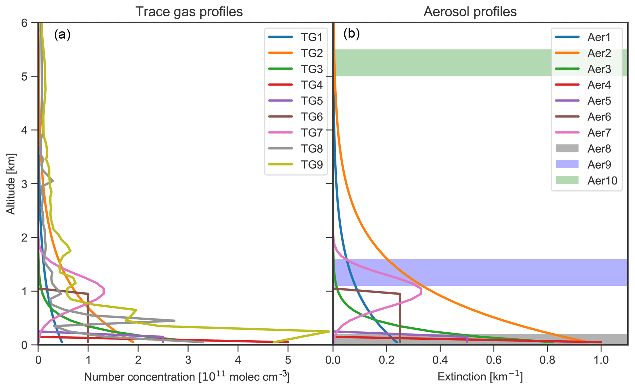
Figure 2Trace gas number concentration (a) and aerosol extinction (b) vertical profiles as input for the forward modelling of HCHO, NO2, and O4. The shaded areas in (b) indicate the location of fog and cloud layers with an extinction coefficient of 10 km−1. The properties of the individual profiles are described in Tables 2 and 3.
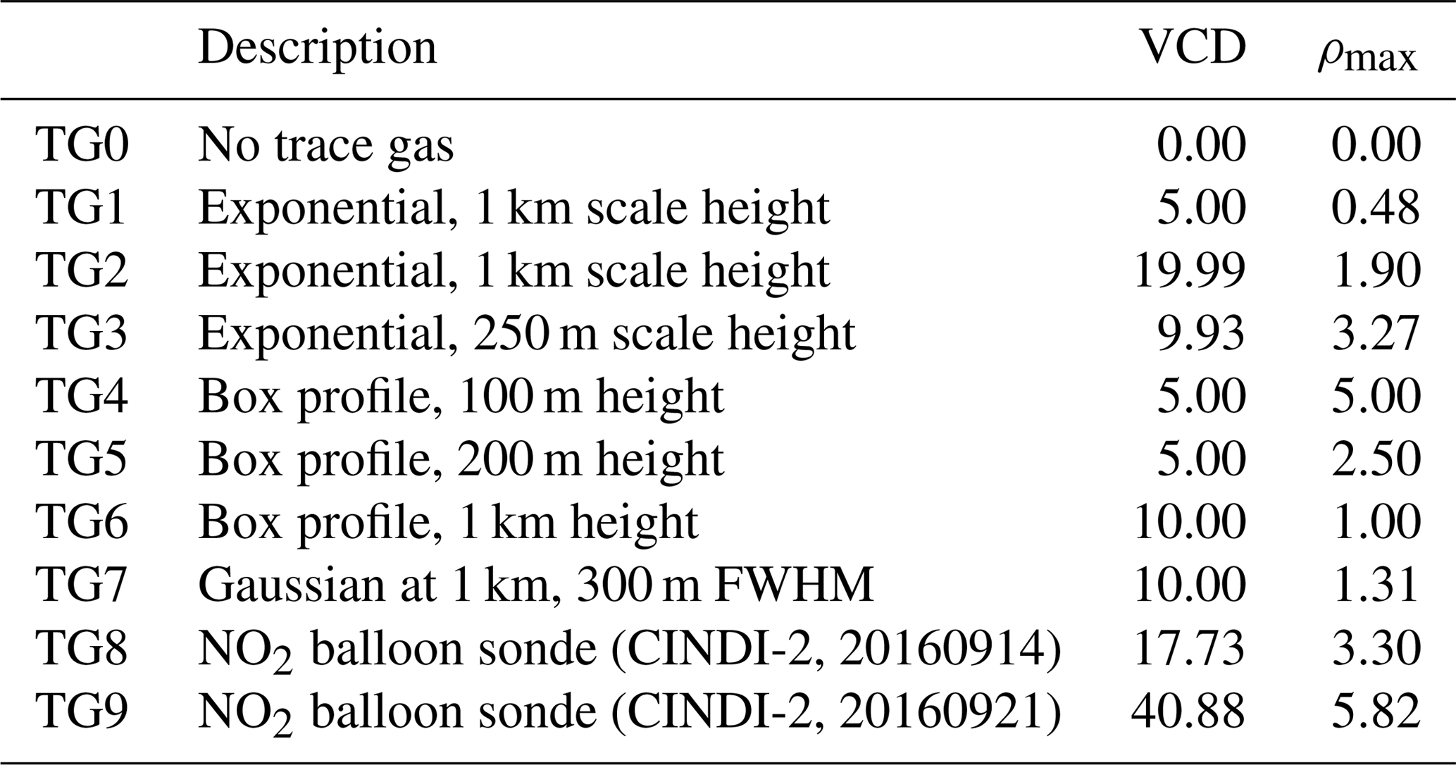
The trace gas concentration and aerosol extinction profile scenarios for the forward modelling of HCHO, NO2 and O4 SCDs are shown in Fig. 2. The same set of trace gas profiles is assumed for both HCHO and NO2, in accordance with ambient measurements in mid-latitudes, where typical concentrations of both species are of the same order of magnitude (e.g. Vlemmix et al., 2015b). For simplicity, it is assumed that aerosol extinction does not change with wavelength (Ångström exponent of zero). The model profiles are chosen in order to represent a large variety of different atmospheric conditions, including trace gas and aerosol free atmospheres as well as moderate to high trace gas and aerosol loads up to cloudy and foggy conditions. The shapes of the different profiles include near-surface box profiles, profiles exponentially decreasing with altitude, uplifted profiles with a Gaussian shape, and profiles without trace gases and aerosols. Additionally, the trace gas scenarios include two NO2 profiles measured with a balloon sonde during the CINDI-2 campaign conducted in the Netherlands in September 2016 (Kreher et al., 2019; see also http://www.tropomi.eu/data-products/cindi-2, last access: 8 April 2019). The aerosol scenarios include three extreme cases with an extinction of 10 km−1 located at the surface, as well as at altitudes around 1.3 and 5.25 km, representing fog and low-lying and high-lying clouds, respectively. In total, the scenarios include 10 trace gas and 11 aerosol profiles whose features are listed in Tables 2 and 3, respectively. The forward calculations of O4 at 360 and 477 nm are performed for each of the 11 aerosol profiles. NO2 and HCHO SCDs are simulated for each combination of aerosol and trace gas profiles, yielding in total 110 different trace gas scenarios.
Table 2Description of the trace gas profiles shown in Fig. 2. The VCD and the maximum number concentration ρmax are given in units of 1015 molec cm−2 and 1011 molec cm−3, respectively.
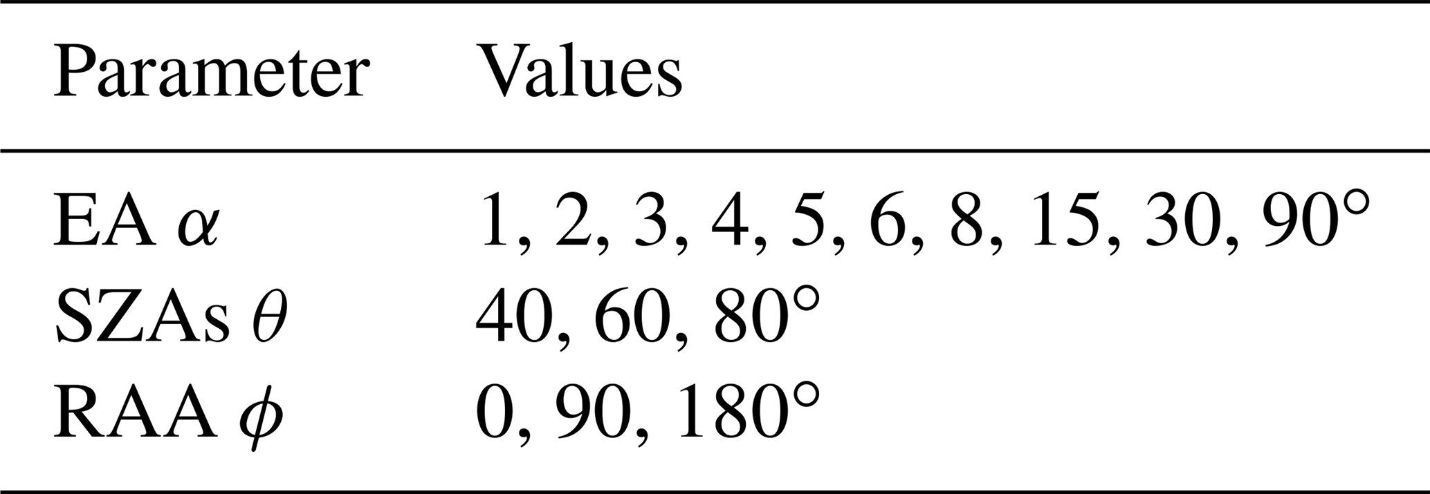
The viewing geometry for the forward model simulations is specified by the EA α, the SZAs θ, and the RAA ϕ between the Sun and the viewing direction of the instrument. Simulations are performed using any combination of values for EA, SZAs, and RAA as listed in Table 4. The EA sequence, consisting of 10 angles between the horizon and zenith, is identical to the measurement sequence during the CINDI-2 campaign. Together with three SZAs and three RAA values, this yields 90 different viewing geometries to be simulated for each model atmosphere.
Table 3Description of the aerosol extinction profiles shown in Fig. 2. The maximum extinction kmax is given per kilometre.
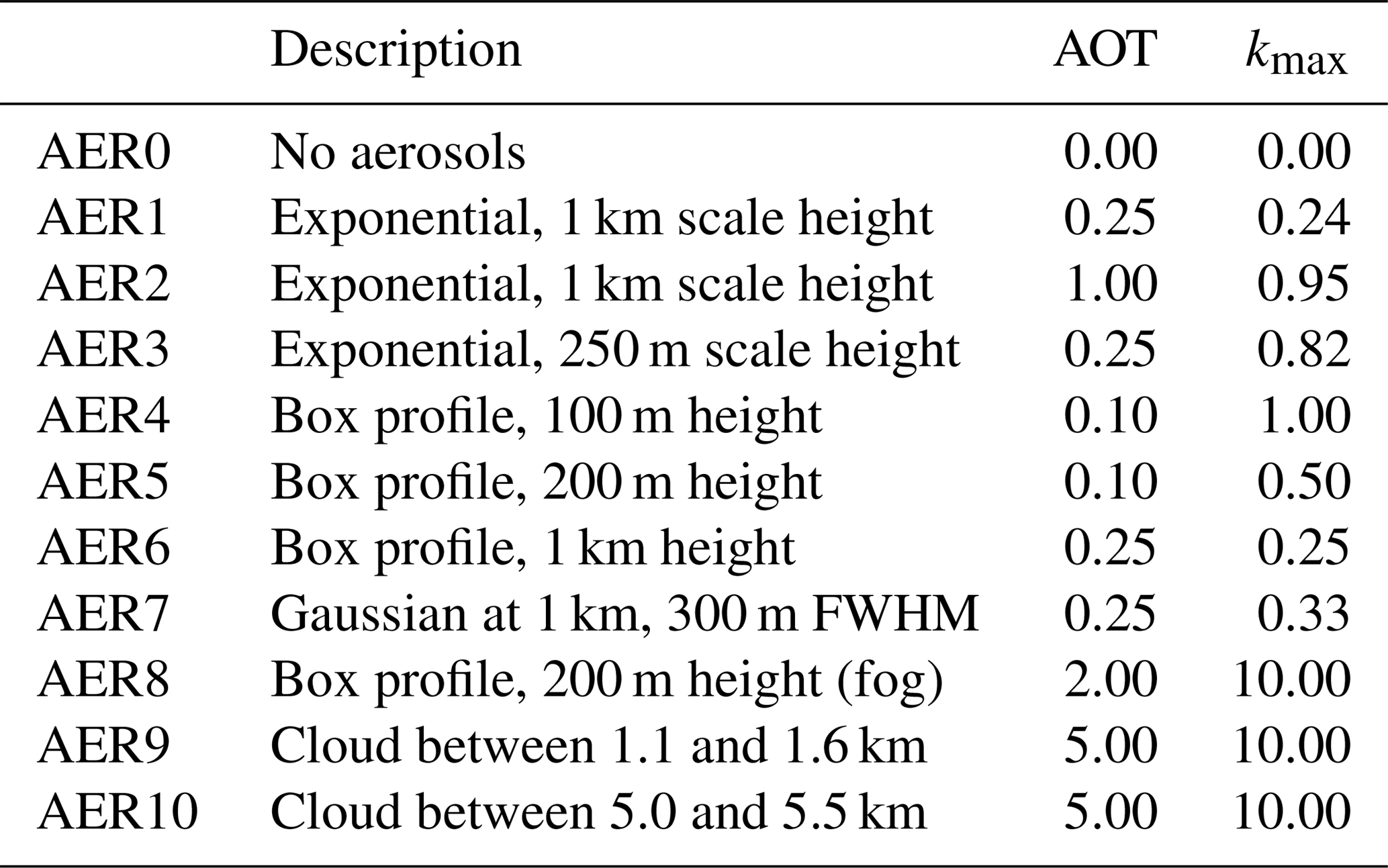
Table 4Viewing geometry for the model calculations. SCDs are simulated for each combination of EA, SZAs, and RAA.
Further RTM parameters specified for both forward and inverse modelling are listed in Table 5, and the wavelengths for the simulation of the different trace gases can be found in Table 6. The RTM parameters include vertical profiles of temperature and pressure derived from average ozone-sondes for the month of September from 2013 to 2015 in De Bilt, the Netherlands, as well as surface albedo, aerosol optical properties, and trace gas literature absorption cross sections. The aerosol scattering was parametrised using a Henyey–Greenstein phase function (Henyey and Greenstein, 1941) with the asymmetry parameter as listed in Table 5.
(Thalman and Volkamer, 2013)(Vandaele et al., 1998)(Meller and Moortgat, 2000)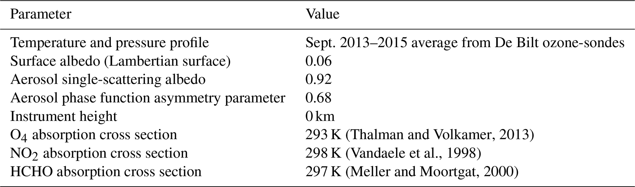
Table 6Assumed measurement errors of the O4, HCHO, and NO2 dSCDs, as well as total columns of the respective a priori profiles. Units for the errors are molec2 cm−5 for O4 and molec cm−2 for HCHO and NO2.

In total, all combinations of viewing geometries, aerosol profiles, and trace gas profiles yield 990 O4 SCD simulations each at 360 and 477 nm and 9900 simulations for each of the trace gases NO2 and HCHO.
In this section, the ability of the forward models to realistically simulate trace gas SCDs is assessed based on a comparison of the individual simulations with the median of the SCDs from the different RTMs. The median SCDs also serve as a reference dataset and provide the synthetic measurements for the profile retrieval comparison presented in Sect. 6. Figure 3 shows the comparison of the simulated O4, NO2, and HCHO SCDs to the respective ensemble median. The respective parameters of a linear regression of forward modelled SCDs versus median SCDs are shown in Fig. 4. The SCDs simulated by most forward models agree under all conditions, with Pearson's coefficients and slopes very close to unity (R>0.999 and ) for a regression between SCDs from the individual models and the median from all models. Exceptions are HEIPRO and PRIAM, both using an older version of the SCIATRAN RTM (version 2.1) as the forward model. These models show deviations for the fog and cloud scenarios (AER8 … AER10), the shallow box profile (AER4), and in the case of HEIPRO also for the exponential profile AER2 with a high AOT of 1. MAPA with McARTIM as the forward model yields significantly smaller slopes of 0.955 and 0.959 than the other models for O4 at 477 nm and for NO2, respectively. This is probably due to the different treatment of sphericity within the McARTIM model. Significant biases are found for MAPA–McARTIM and PRIAM–SCIATRAN for NO2 and O4 at 477 nm, as well as for HEIPRO–SCIATRAN for HCHO. Apart from possible differences in the implementation and the approaches of the individual RTMs, some of the differences are likely due to the different representations of the trace gas and aerosol profiles on the prescribed vertical grid.

Figure 3Correlation of SCDs of O4 (360 and 477 nm), HCHO, and NO2 simulated by the different forward models with the corresponding median SCDs from all models. Colours indicate the underlying aerosol and trace gas profiles as denoted in the legend. For HCHO and NO2, results for all scenarios with different aerosol profiles are included.
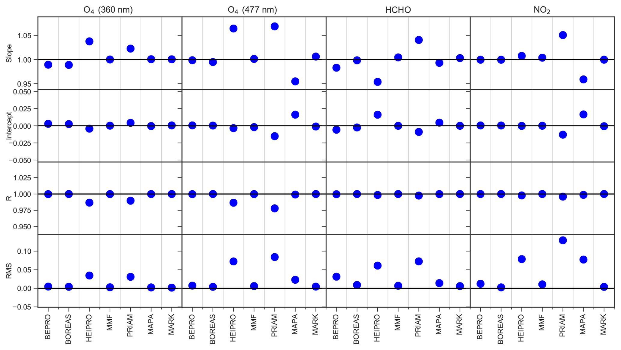
Figure 4Slope, intercept, regression coefficient, and root-mean-square difference (RMS) of the correlation between the SCDs from the individual forward models and the median SCDs from all models. RMS and intercept values are in units of 1043 molec2 cm−5 for O4 and 1017 molec cm−2 for HCHO and NO2.
In summary, the SCDs simulated by the different radiative transfer models agree well under all conditions, as within previous RTM intercomparisons (e.g. Wagner et al., 2007). This implies that possible discrepancies in the retrieved trace gas and aerosol profiles are mainly caused by differences in the implementation of the retrieval algorithms, rather than by differences in the forward models.
This section presents the results of the aerosol and trace gas retrieval algorithm intercomparison. Section 6.1 describes the measurement vectors, forward model parameters, and a priori constraints of the profile retrieval. An important diagnostic tool is provided by the AVKs from the OEM algorithms, which quantify the sensitivity of the retrieval to the atmospheric state. AVKs and information content are discussed in Sect. 6.2. The comparison of modelled and measured dSCDs presented in Sect. 6.3 provides a measure for the level of convergence of the retrieval algorithms. Results of the intercomparison of vertical profiles, trace gas and aerosol total columns, and surface extinction and trace gas concentrations are presented in Sect. 6.4, 6.5, and 6.6, respectively. Finally, the computational speed of the retrieval algorithms is discussed in Sect. 6.7.
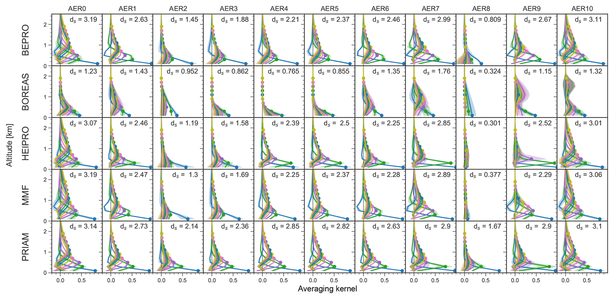
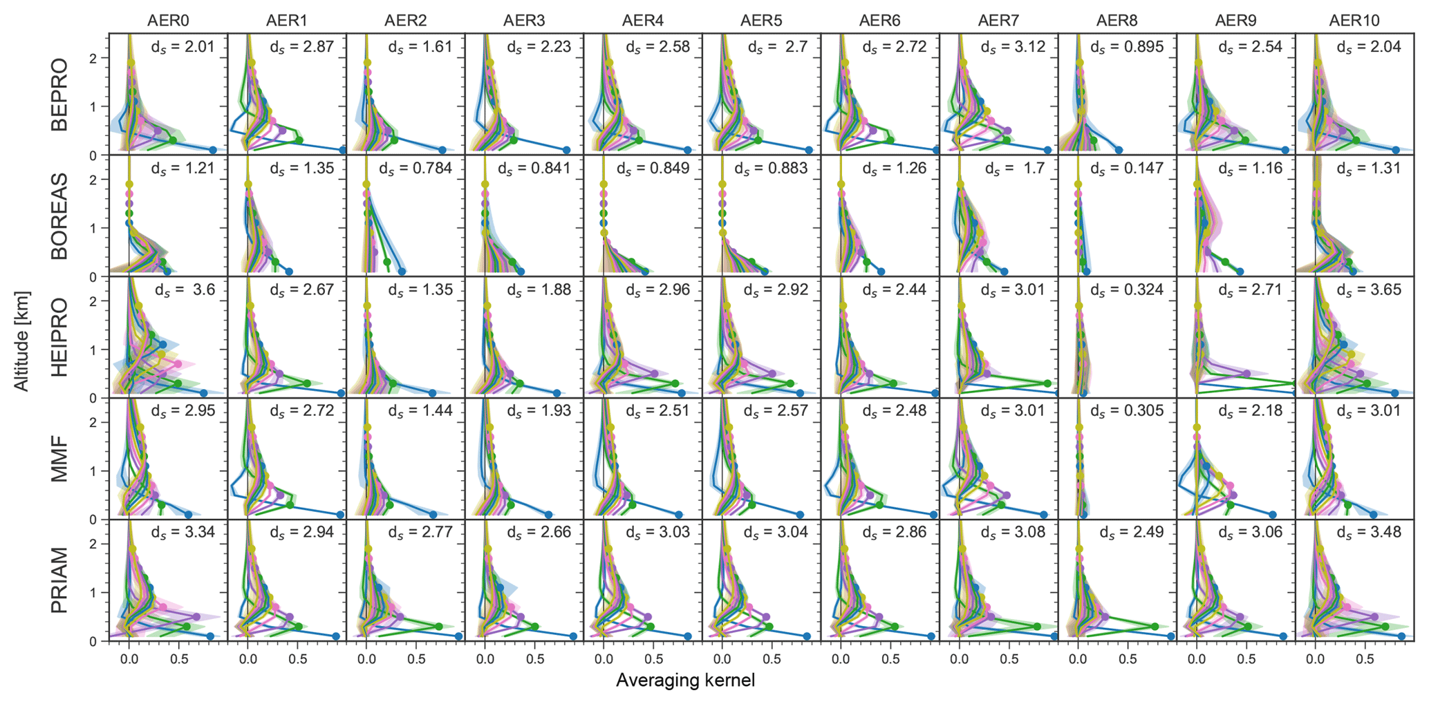
Figure 5The 360 nm aerosol AVKs. Each subplot shows the mean AVK over all SZAs and RAA for a specific aerosol scenario (columns) and retrieval algorithm (rows). Filled circles indicate the nominal altitude of the corresponding AVK plotted in the same colour. Colour-shaded areas (barely visible in most cases) indicate the standard deviation of the AVKs, i.e. the variation for different SZAs and RAA. Also shown are the DFS. AVKs stem from retrievals with noisy measurements (v1n).
6.1 Retrieval settings
Based on the simulated SCDs from the atmospheric scenarios described in Sect. 5, a reference dataset of O4 at 360 and 477 nm, NO2, and HCHO dSCDs has been compiled based on the ensemble median dSCDs from all participants. In the following, we refer to this synthetic dataset as the measured dSCDs. Table 6 lists the according dSCD errors, which were chosen to represent typical values based on ambient measurements by various instruments during the CINDI-2 campaign. As already discussed in Sect. 4, the reference dataset contains dSCDs at nine EAs for 990 different combinations of trace gas profiles, aerosol profiles, and solar geometry (SZAs and RAA).
Two reference datasets were created: dataset v1 contains the median dSCDs without any noise, and dataset v1n contains the median dSCDs with a noise component consisting of the sum of (1) normally distributed noise with a standard deviation according to the errors listed in Table 6, and (2) additional noise with a standard deviation of 5 % of the dSCD values. This second noise component, which is in the case of O4 and NO2 much higher than typical measurement noise, is supposed to represent random variations in the measured dSCDs due to horizontal inhomogeneities of aerosols and trace gases as well as temporal changes in the atmospheric state (in particular cloud properties) during a single elevation scan with a typical duration of several minutes. The second noise component is of magnitude similar to the RMS differences between dSCDs measured by more than 30 instruments during the CINDI-2 Campaign (Kreher et al., 2019).
Each participant performed retrievals with settings being as close as possible to the prescribed settings described below. The results based on noise-free and noisy dSCDs are labelled “v1” and “v1n”, respectively. Each measurement vector consists of O4, HCHO, or NO2 dSCDs of a single EA sequence for a given atmospheric scenario specified by aerosol and trace gas profiles, as well as solar zenith and relative azimuth angles. Retrievals are performed using the same forward model parameters as for the forward model calculations (see Table 5), with the exception of MAPA that uses slightly different surface albedo and aerosol optical properties (see Sect. 3.6). The retrieval grid consists of 20 layers with 200 m in thickness between the surface and 4 km in altitude, which means that the atmospheric layers are twice as thick as for the forward modelling. This choice allows for the investigation of the impact of sub-grid variations on the retrieval, in particular in the case of scenarios TG4 and AER4 (100 m thick box profiles).
In contrast to the output of OEM algorithms, which directly retrieve trace gas and aerosol profiles on this vertical grid, profiles from the parametrised algorithms are interpolated onto the prescribed grid. The OEM algorithms use aerosol and trace gas a priori profiles exponentially decreasing with altitude with a scale height of 1 km, with a priori vertical columns for each species as listed in Table 6. The diagonal elements of the a priori covariance matrices consist of the square of 50 % of the corresponding a priori profiles. Off-diagonal terms consist of a Gaussian function with a correlation length of 200 m as described by Clémer et al. (2010).
Optionally, each participant can define criteria for the validity of the retrieved profiles, and can provide corresponding Boolean validity flags for each profile.
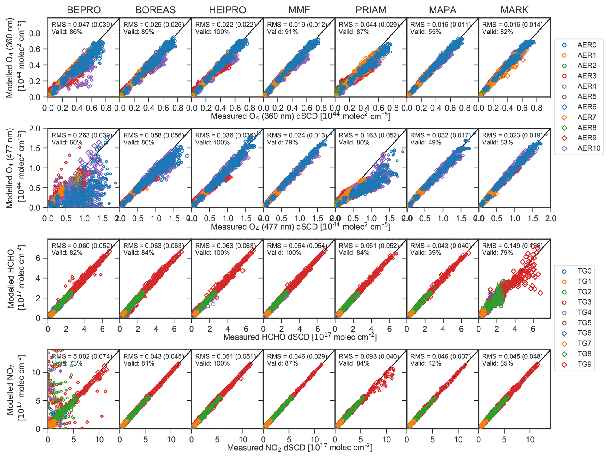
Figure 9A posteriori versus measured dSCDs of O4 (360 and 477 nm), HCHO, and NO2 for the v1n dataset. Colours and symbols indicate the underlying aerosol and trace gas profiles, respectively, as denoted in the legend. Data flagged as invalid are shown as smaller symbols. Also shown are the RMS differences between measured and modelled dSCDs with the RMS for valid data only being shown in brackets, as well as the percentage of valid data. Units of the RMS are 1044 molec2 cm−5 for O4 and 1017 molec cm−2 for HCHO and NO2.
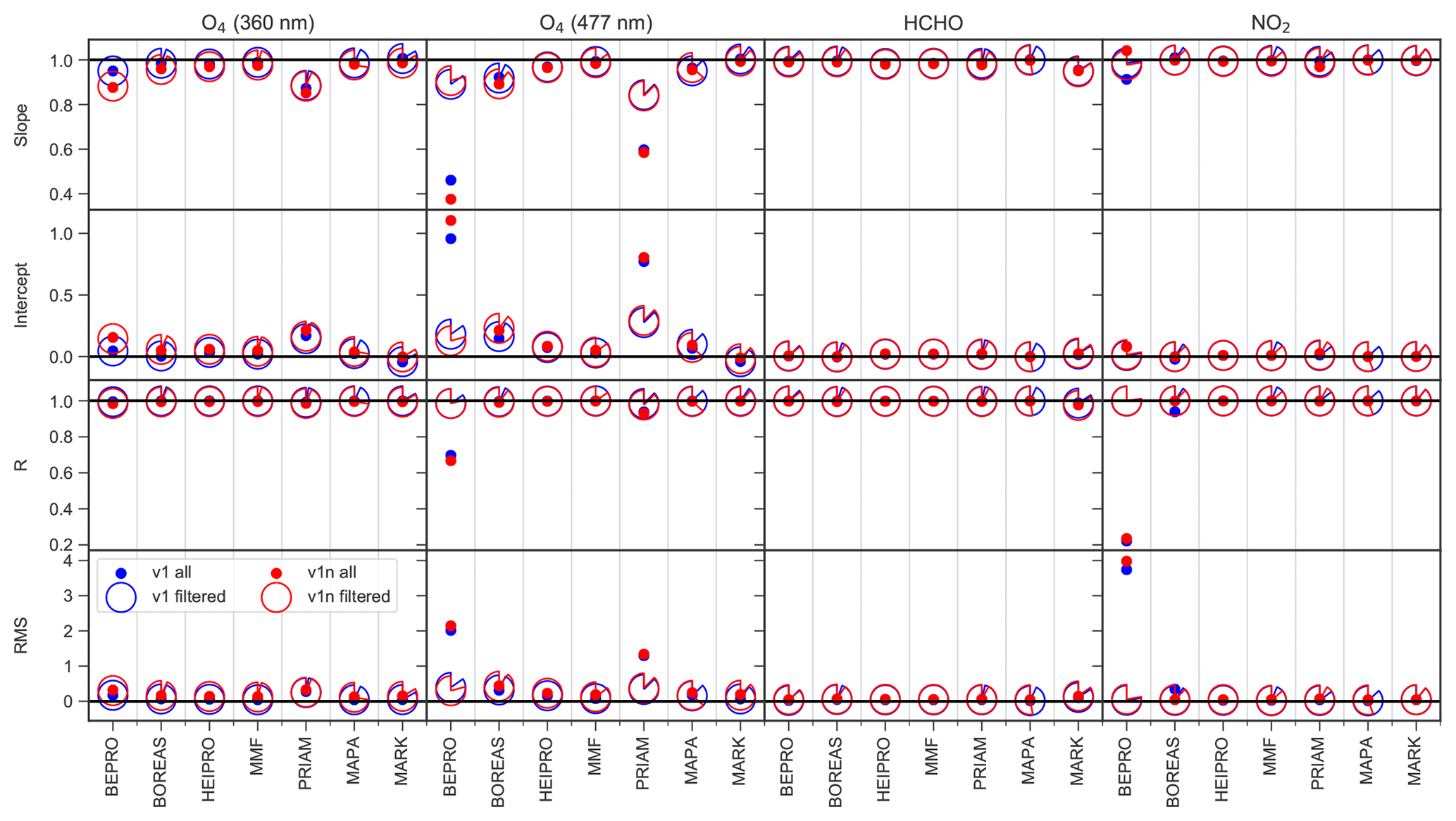
Figure 10Slope, intercept, regression coefficient, and RMS of the dSCD correlation. Each of the circular symbols for the filtered data represents a pie chart that quantifies the fraction of data flagged as valid. RMS and intercept values are in units of 1043 molec2 cm−5 for O4 and 1017 molec cm−2 for HCHO and NO2. Cloud and fog scenarios (AER8, AER9, AER10) are excluded from the regression analysis.
6.2 Comparison of averaging kernels
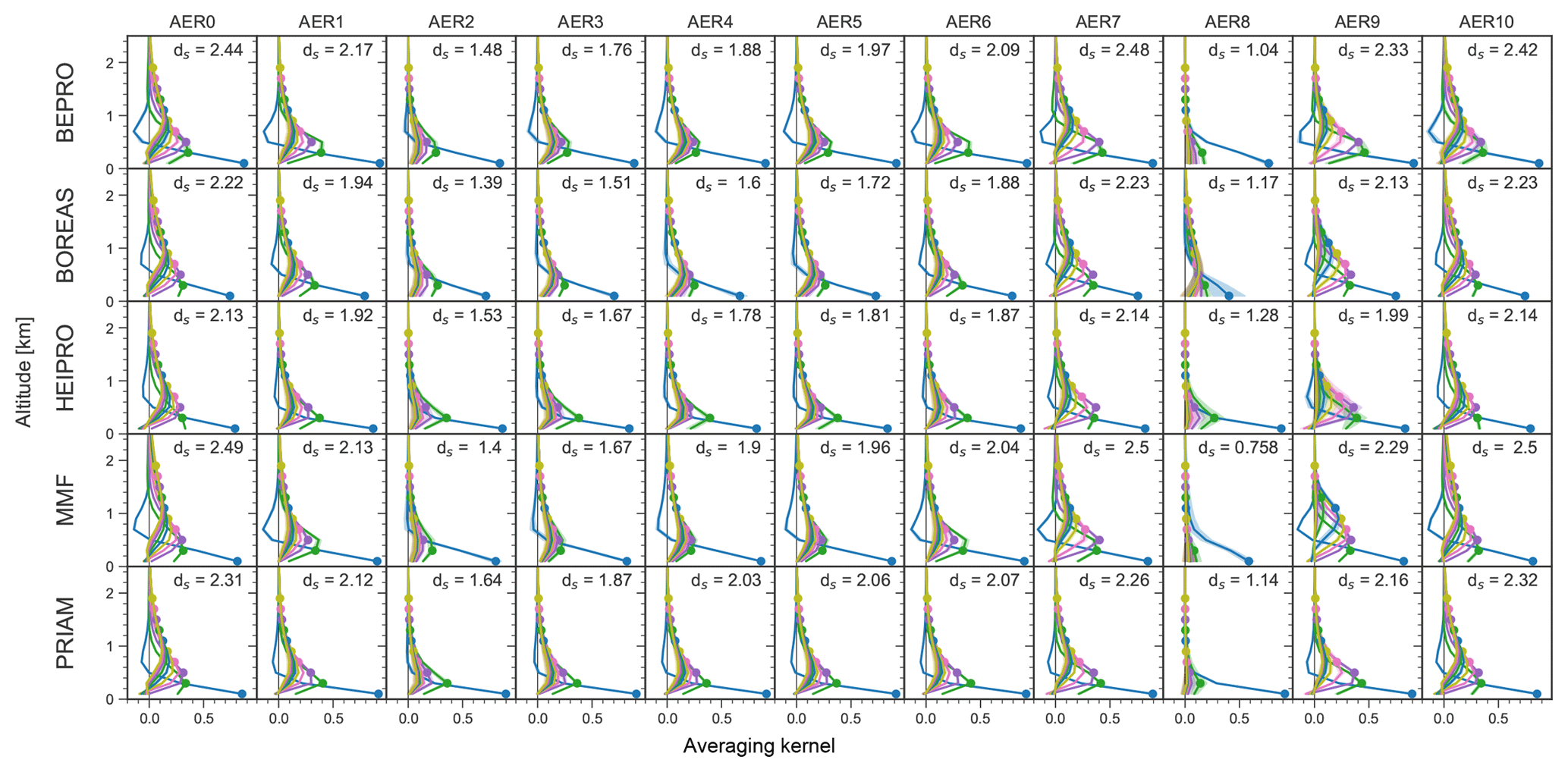
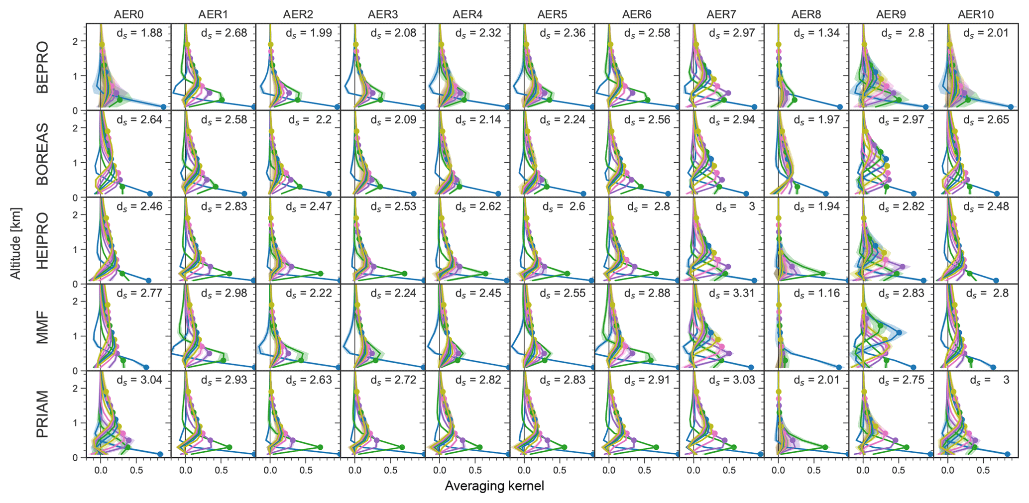
Figures 5, 6, 7, and 8 show the AVKs from the OEM algorithms for aerosols at 360 and 477 nm, HCHO, and NO2, respectively. The AVKs confirm that MAX-DOAS measurements yield only information on the lowermost ≈2 km of the atmosphere when using a zenith-sky reference spectrum from the same EA sequence. This is a result of the measurement geometry and, in the case of aerosols, also of the fact that the O4 vertical distribution is heavily weighted to the surface. The DFS range from ds<0.5 during foggy conditions (AER8) to ds>3 for aerosol-free atmospheres (AER0), with the information content being generally higher for aerosols than for trace gases. The dependency of the information content on wavelength is inconsistent: for a pure Rayleigh atmosphere (AER0), bePRO, BOREAS, and MMF report smaller DFS for aerosols at 477 nm than at 360 nm, while the opposite is true for HEIPRO and PRIAM. The information content for trace gases increases with wavelength for all algorithms, except for bePRO in the case of the AER0 scenario.
The shapes of the AVKs from the different models have a high degree of similarity, except for BOREAS aerosols, where the AVKs show a much smaller information content than all other algorithms and indicate that there is very little height sensitivity for aerosol profiles from the BOREAS algorithm. The respective BOREAS aerosol vertical profiles are, however, in good agreement with the results from the other algorithms (see Sect. 6.4). The reason for this apparent discrepancy is that BOREAS is not a standard OEM retrieval but includes additional regularisation terms, making interpretation of the AVKs less straightforward (Bösch et al., 2018). Significant differences between the AVKs can be found for the rather extreme scenarios AER8 and AER9 (fog and low-lying cloud). PRIAM aerosol AVKs are much less affected by fog (AER8) than the other algorithms, which show a strong reduction in information content in the case of high extinction at the surface. The AVKs for a high-lying cloud at ≈5 km in altitude (AER10) are very similar to those of a Rayleigh atmosphere (AER0), indicating that horizontally homogeneous free tropospheric clouds have little impact on the sensitivity of MAX-DOAS retrievals.
Apart from the fog scenario (AER8), there is only a moderate dependency of vertical resolution and information content on the aerosol content of the atmosphere. Interestingly, the information content for trace gases, in particular NO2, is highest for the uplifted aerosol layer (AER7). This layer probably increases the sensitivity for trace gases near the surface due to the fact that the majority of scattering occurs within the cloud. The light paths below the cloud are thus well defined and, in the case of low EAs, can be higher than for the clear-sky case.
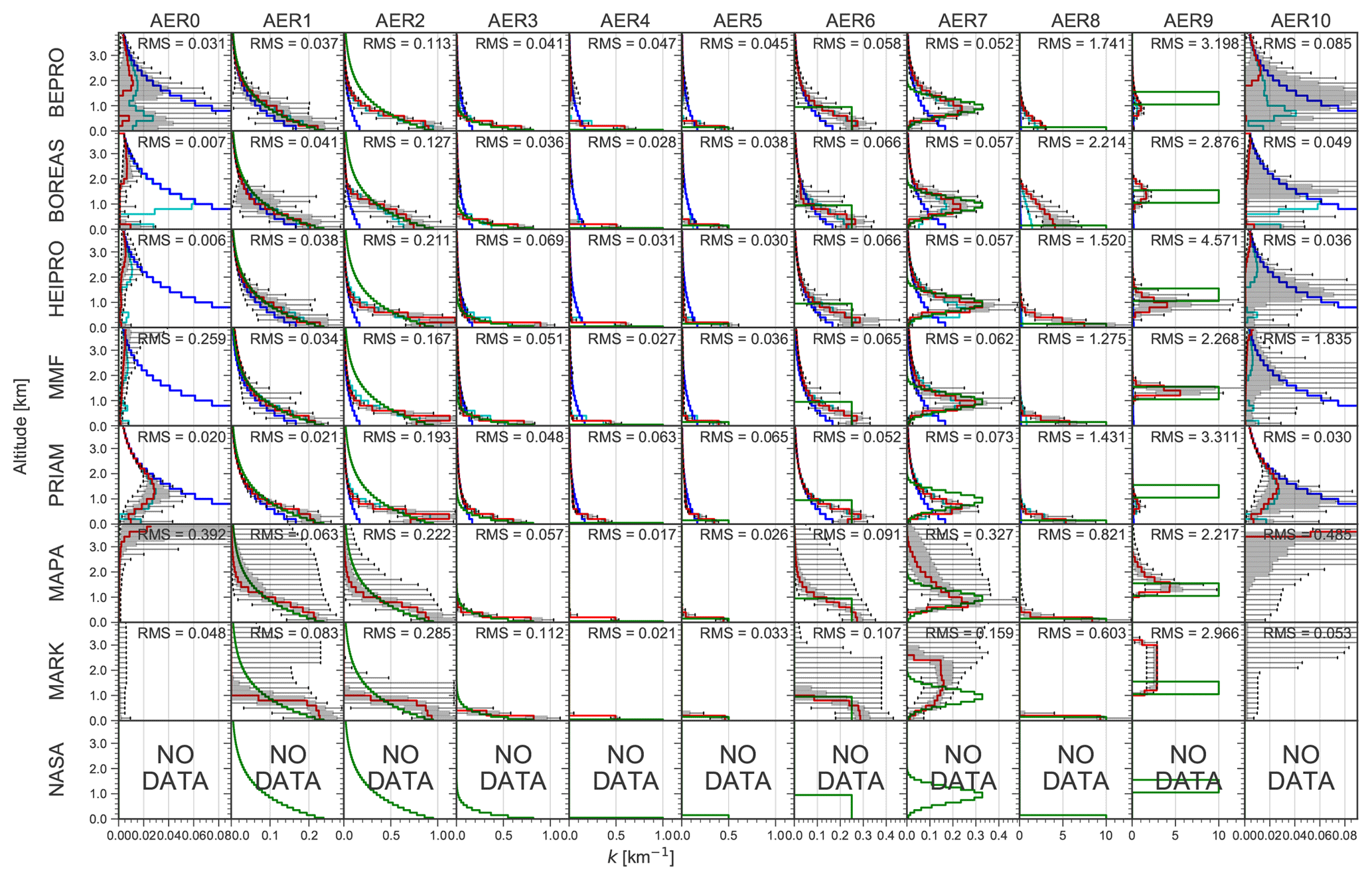
Figure 11Comparison of retrieved (red solid line, version v1n) and true (green solid line) vertical profiles of aerosol extinction at 360 nm for each aerosol scenario (columns) and algorithm (rows). The retrieved profiles are the medians for all SZA–RAA combinations. The (25 %–75 %) and (5 %–95 %) percentiles are shown as grey areas and whiskers, respectively. The a priori profile is shown as the blue line (OEM algorithms only).
The variability of the AVKs with the position of the Sun (shown as shaded areas in Figs. 6–8) is generally very small, indicating little dependency on SZAs and RAA.
6.3 Comparison of a posteriori dSCDs
An important indicator for the level of convergence of the retrieval, and subsequently the accuracy of the retrieved profile, is the agreement between the measurement vector y and the measurement vector modelled for the retrieved state (a posteriori dSCDs). The comparison of a posteriori and measured dSCDs for the v1n dataset is shown in Fig. 9, and the corresponding linear regression parameters are depicted in Fig. 10. The NASA algorithm does not rely on the forward modelling of dSCDs; thus no dSCD data are available for this algorithm.
The algorithms show significant differences in the level of convergence. BOREAS, HEIPRO, MMF, and MAPA show good agreement between measured and modelled dSCDs for all scenarios with slopes and Pearson correlation coefficients close to unity. The same holds true for MARK except for the HCHO retrieval, where poor convergence is achieved for the TG9 scenario, but this has only a little effect on the regression parameters (see Fig. 10). PRIAM achieves good convergence for the trace gas retrievals, but shows a larger scatter than other algorithms for O4 at 360 nm and significantly underestimates O4 at 477 nm, where the slope of the linear regression is only 0.585. In many cases, bePRO yields only poor agreement between measured and modelled dSCDs, in particular in the visible range where the RMS between measurement and modelling is significantly higher than for the other algorithms, and regression coefficients are only 0.67 for O4 dSCDs and 0.24 for NO2 dSCDs. The bePRO algorithm furthermore has problems retrieving the AER10 scenario (high-lying cloud) at 360 nm. The poor convergence of the bePRO algorithm is the result of numerous outliers, and the RMS strongly improves after discarding about 15 % of the 477 nm O4 data points and 23 % of the NO2 data points that are flagged as invalid. The reason for the instabilities of the bePRO algorithm, which strongly affect the accuracy of the retrieved profiles (see Sect. 6.4), is the fact that bePRO uses a Gauss–Newton inversion scheme. Sensitivity studies have shown that this problem could be overcome by using a Levenberg–Marquardt inversion scheme instead. More than 55 % of data from MAPA are flagged as invalid although the retrievals show a high level of convergence. This might indicate that the MAPA quality flagging criteria could be too strict.
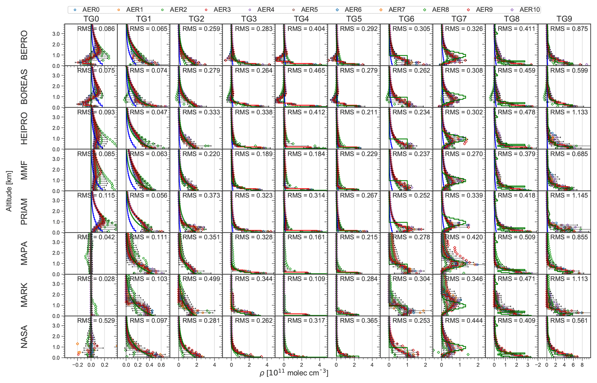
Figure 13Comparison of retrieved (red solid line, version v1n) and true (green solid line) vertical profiles of HCHO for each trace gas scenario (columns) and algorithm (rows). In addition to the median profiles for all aerosol scenarios, SZAs and SAAs shown in red, the median concentration profile for each aerosol scenario is shown as coloured symbols as denoted in the legend. The RMS (true – retrieved extinction) is shown in units of 1011 molec cm−3.
6.4 Comparison of vertical profiles
In this section, the overall ability of the retrieval algorithms to reproduce the true atmospheric aerosol and trace gas profiles is discussed. Figures 11 and 12 show the comparison between true and retrieved aerosol profiles at 360 and 477 nm, and HCHO and NO2 profile comparisons are shown in Figs. 13 and 14, respectively. The regression parameters for the comparison of true and retrieved aerosol extinction and trace gas number concentration for all target species are presented in Fig. 15. All data presented here are based on retrievals with noisy dSCDs (v1n). The corresponding profiles with valid data only, and with noise-free measurements, are shown in the Supplement.
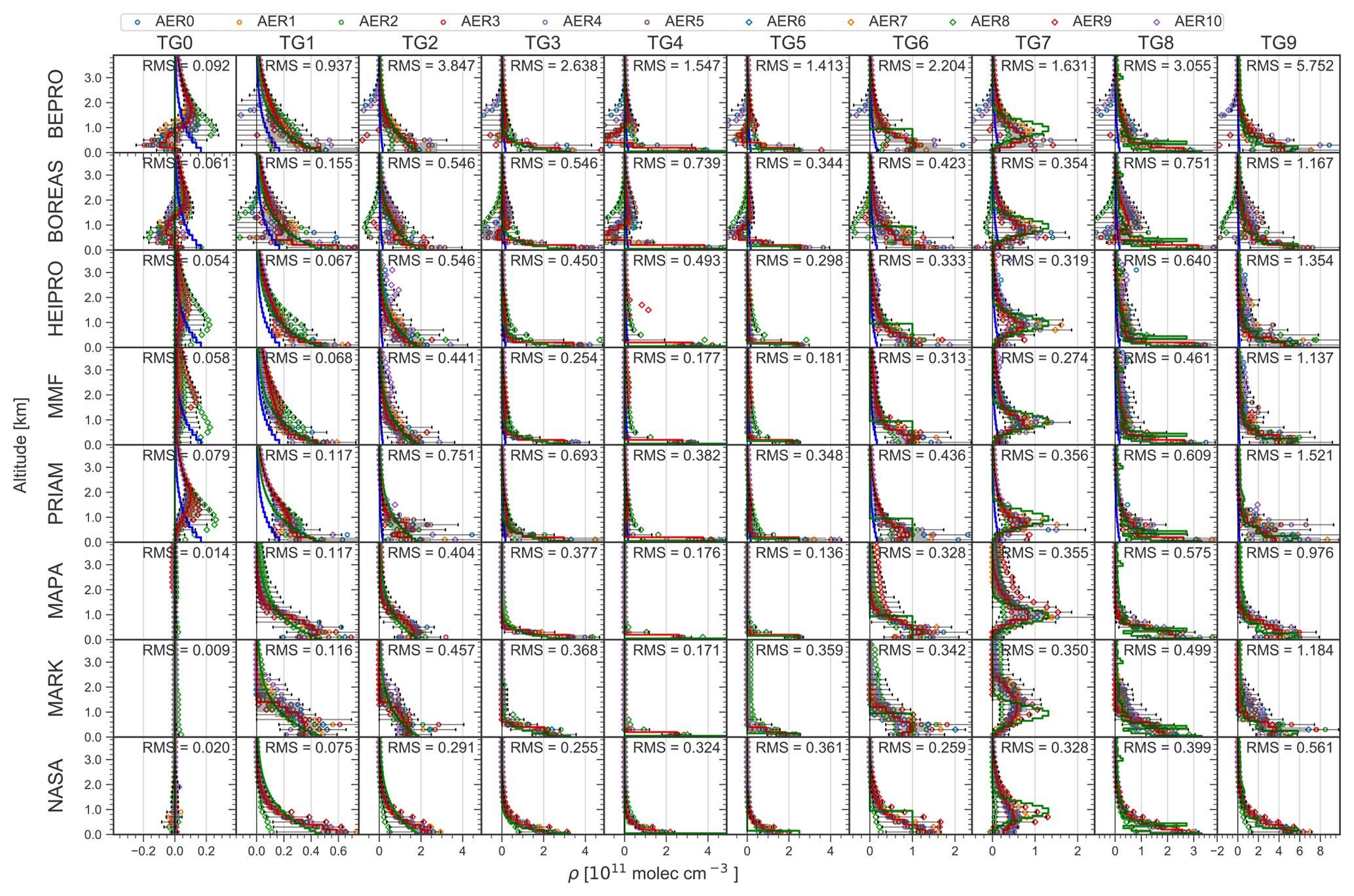
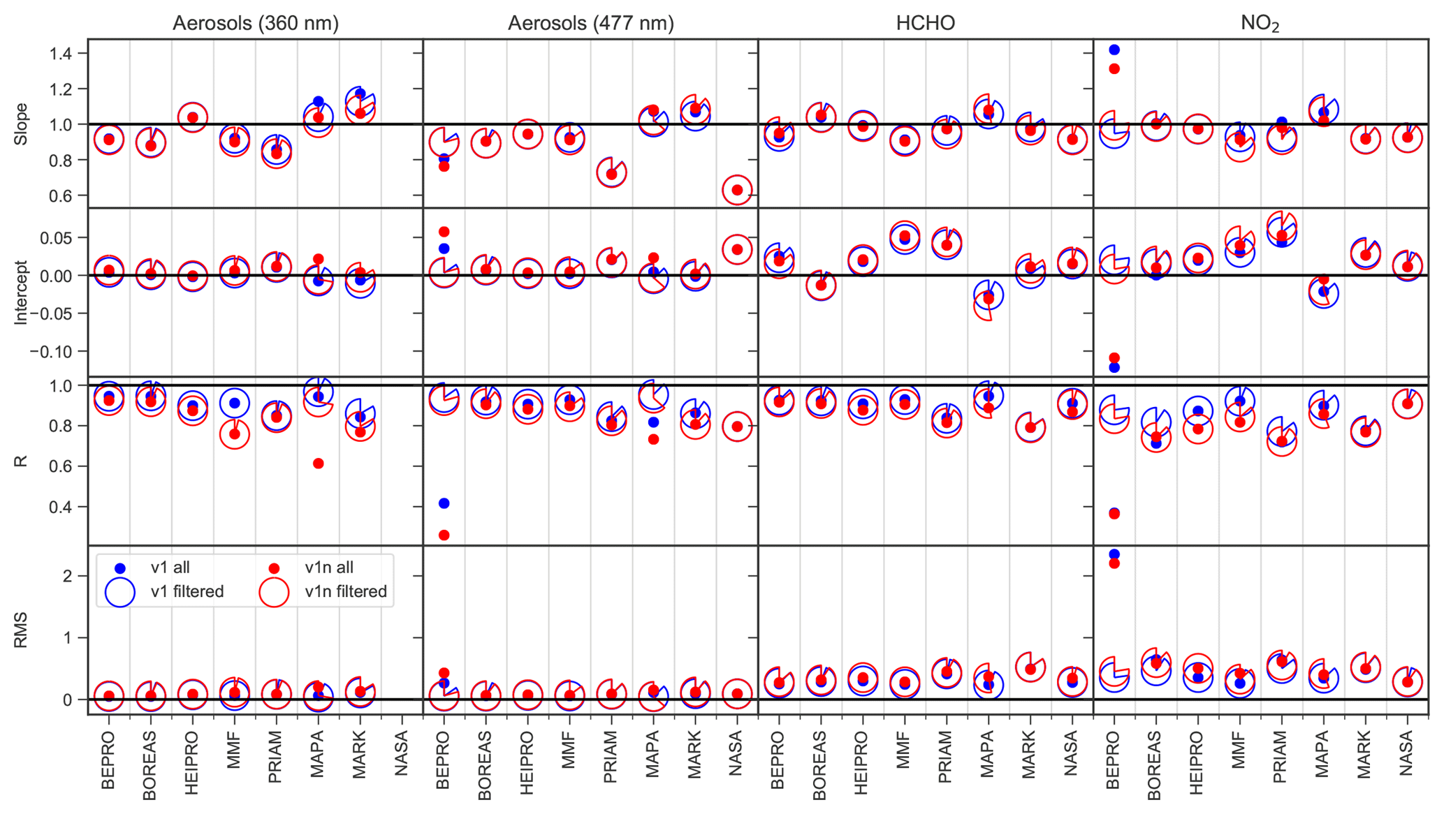
Figure 15Slope, intercept, regression coefficient, and RMS for the correlation between true and retrieved aerosol extinction as well as HCHO and NO2 number concentrations at all altitudes. Intercept and RMS values are per kilometre for aerosols and 1011 molec cm−3 for HCHO and NO2. Cloud and fog scenarios (AER8, AER9, AER10) are excluded from the regression analysis.
Most algorithms are capable of realistically retrieving the shape of the true aerosol extinction profiles for moderate conditions (AER0 … AER7), with slopes close to unity and Pearson regression coefficients for the correlation between true and retrieved extinction of R>0.8 (see Fig. 15). Exponential profiles (AER1, AER2, and AER3) are well reproduced, but the extinction above ≈1 km is underestimated by all algorithms for AER2 (high aerosols, exponentially decreasing) owing to a reduced sensitivity of MAX-DOAS measurements to high altitudes. In the case of OEM algorithms, this leads to a bias towards the a priori as discussed in Sect. 6.2, whereas parametrised algorithms tend to become unstable at altitudes where the sensitivity is low. The shallow aerosol layers AER4 and AER5 are captured well by all algorithms except NASA (which provides profiles at 477 nm only). The retrievals are performed on a 200 m grid, and the 100 m thick layer (AER4) yields results similar to the 200 m thick layer (AER5), which has the same AOT but only half the extinction coefficient. As expected, the 1 km thick aerosol layer AER6 is significantly smoothed by the retrievals, except by MARK, which reproduces the sharp edges of this profile better than the other algorithms. The uplifted Gaussian profile with a centre altitude of 1 km (AER7) is well reproduced by all OEM algorithms, and to a lesser extent also by NASA. The parametrised algorithms MAPA and MARK also retrieve uplifted profiles, but significantly overestimate the extinction above 1 km.
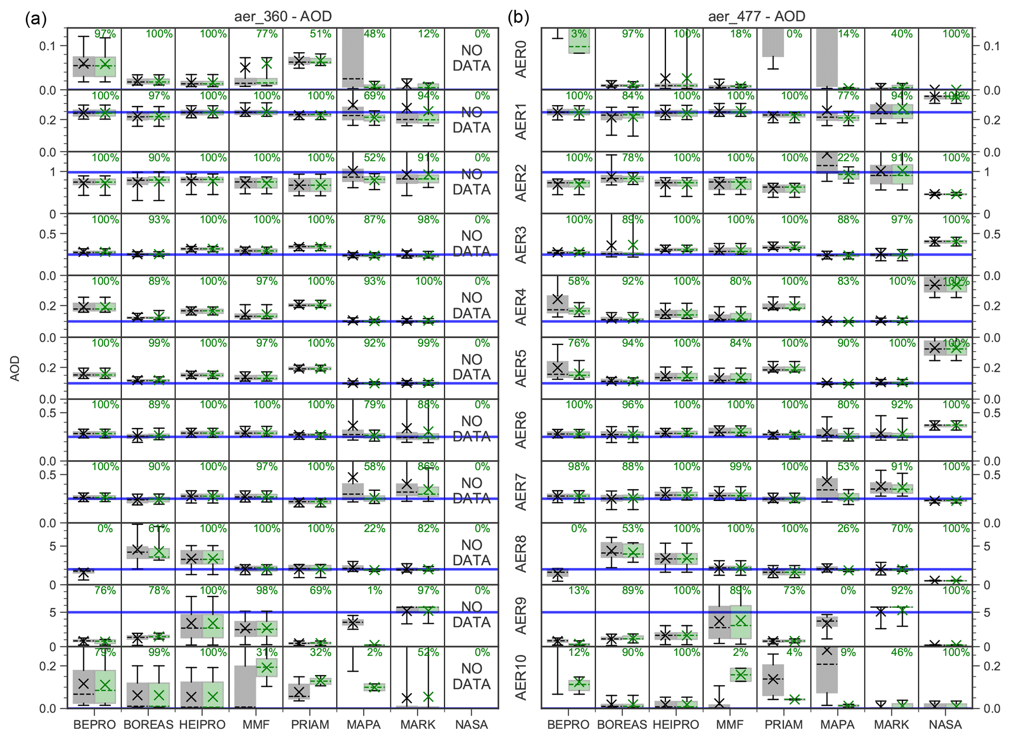
Figure 16Box–whisker plots of the retrieved AOT at 360 (a) and 477 nm (b) for the different aerosol scenarios (rows) and retrieval algorithms (columns) based on retrievals using noisy dSCDs. Crosses show the mean and dashed horizontal lines the median. Shaded areas indicate the (25 %–75 %) percentile, and whiskers show the (5 %–95 %) percentile. The true AOT is shown as the blue horizontal line. For each algorithm, all data are shown on the left in black, and data marked as valid are shown on the right in green. Also shown is the percentage of valid data.
The 200 m thick fog layer (AER8) is very well reproduced by the parametrised algorithms MAPA and MARK, and to a lesser extent also by the OEM algorithms MMF, HEIPRO, and PRIAM, which retrieve the logarithm of the aerosol extinction profile and are therefore capable of retrieving a higher range of aerosol extinction values than bePRO, which operates in linear space and therefore is subject to a stronger bias towards the a priori. The cloud above 1 km (AER9) is very well retrieved by MMF. MAPA and MARK capture the cloud bottom altitude but overestimate the extinction above the cloud. The bePRO, BOREAS, HEIPRO, and PRIAM algorithms retrieve only a small enhancement of the aerosol extinction (<2 km−1) around the altitude of the cloud, and NASA appears to be insensitive to the cloud.
The retrieved extinction profiles for scenario AER10, which consists of a cloud above 5 km altitude and no aerosols elsewhere, are very similar to the cloud- and aerosol-free scenario AER0, although the RMS difference between true and retrieved profiles is higher for AER10 than for AER0 in some cases. As already discussed in Sect. 6.3, measured and a posteriori dSCDs are also in good agreement for AER10. It can therefore be concluded that high-lying clouds have very little effect on MAX-DOAS aerosol retrievals, in contradiction to the findings of Ortega et al. (2016), who suggest that free-tropospheric aerosols and clouds would strongly affect MAX-DOAS measurements of O4.

Figure 17Box–whisker plots of the retrieved HCHO (a) and NO2 (b) VCD for the different trace gas scenarios (rows) and retrieval algorithms (columns) based on retrievals using noisy dSCDs. Crosses show the mean, and dashed horizontal lines show the median. Shaded areas indicate the (25 %–75 %) percentile, and whiskers show the (5 %–95 %) percentile. The true VCD is shown as a blue horizontal line. For each algorithm, all data are shown on the left in black, and data marked as valid are shown on the right in green. Also shown is the percentage of valid data. The median for each aerosol scenario is shown as a coloured symbol as indicated in the legend.
As can be seen from the width of the 50 % and 90 % confidence intervals (shaded areas and error bars in Figs. 11 and 12), the parametrised algorithms (MAPA and MARK) produce a significant number of outliers of the retrieved aerosol profiles, in particular for the scenarios AER1, AER2, AER6, and AER7. This effect is larger for retrievals with noisy than with noise-free dSCDs (see Supplement Figs. S5 and S6). A likely reason for this behaviour is that MAPA and MARK do not rely on a priori constraints as a regularisation, but use a minimisation method for the differences between measured and modelled dSCDs. In some cases the ensemble of possible solutions with similar minima can be widespread. However, in most cases the outliers do not significantly affect the overall accuracy as expressed by the RMS difference between retrieved and true aerosol profiles (see Fig. 15).
Note that for MAPA the spread of the retrieved profiles is far smaller when only filtered results are considered (see Figs. S1–S4), indicating that the MAPA filter is successfully removing outliers. This requires, however, excluding 17 % and 37 % of the aerosol profiles at 360 and 477 nm, respectively, as well as 47 % of the HCHO profiles and 44 % of the NO2 profiles of the AER0–AER7 scenarios, while almost 93 % of the profiles for scenarios with cloud and fog layers (AER8–AER10) are discarded.
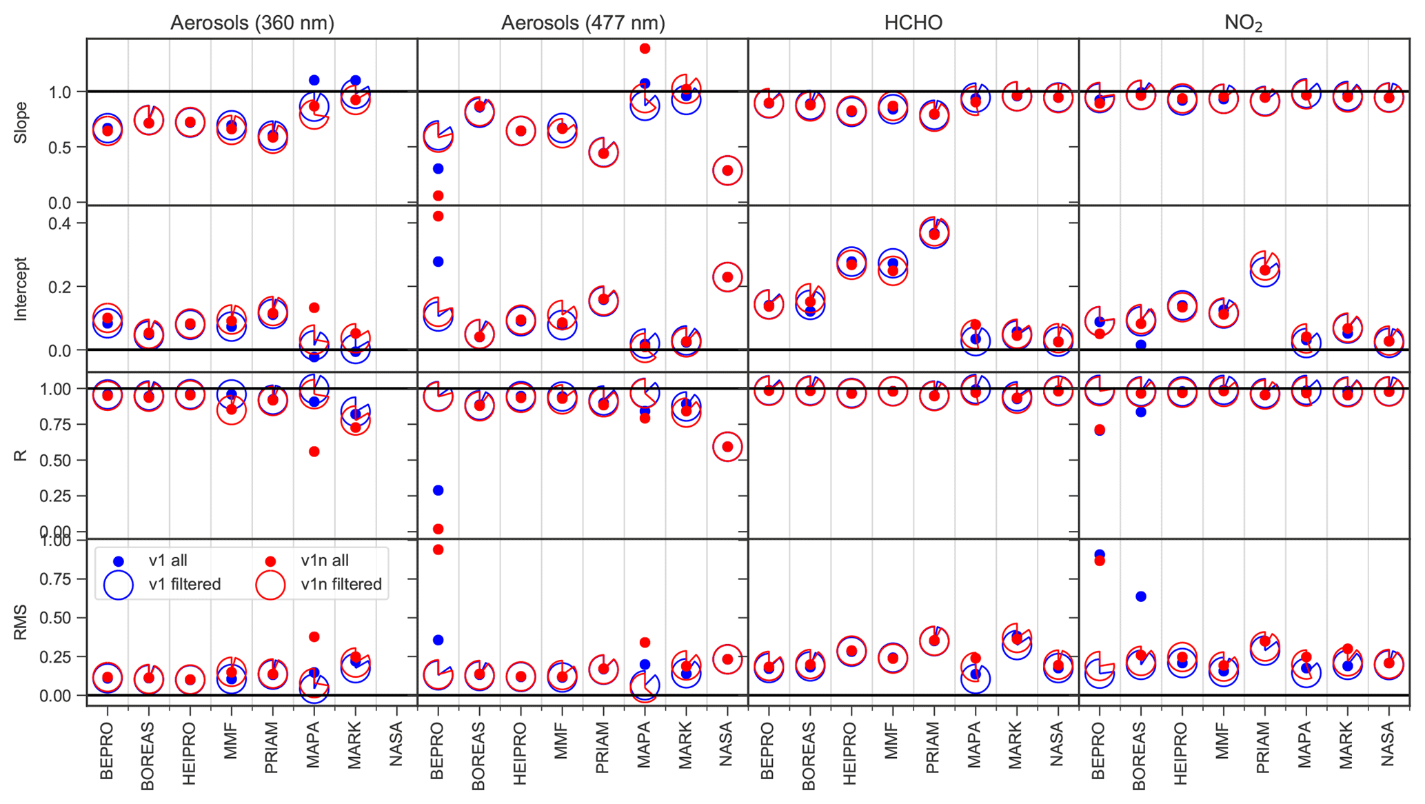
Figure 18Slope, intercept, regression coefficient, and RMS for the correlation between true and retrieved AOT as well as HCHO and NO2 VCD. Intercept and RMS values are in dimensionless units for aerosols and 1016 molec cm−2 for HCHO and NO2. Cloud and fog scenarios (AER8, AER9, AER10) are excluded from the regression analysis.
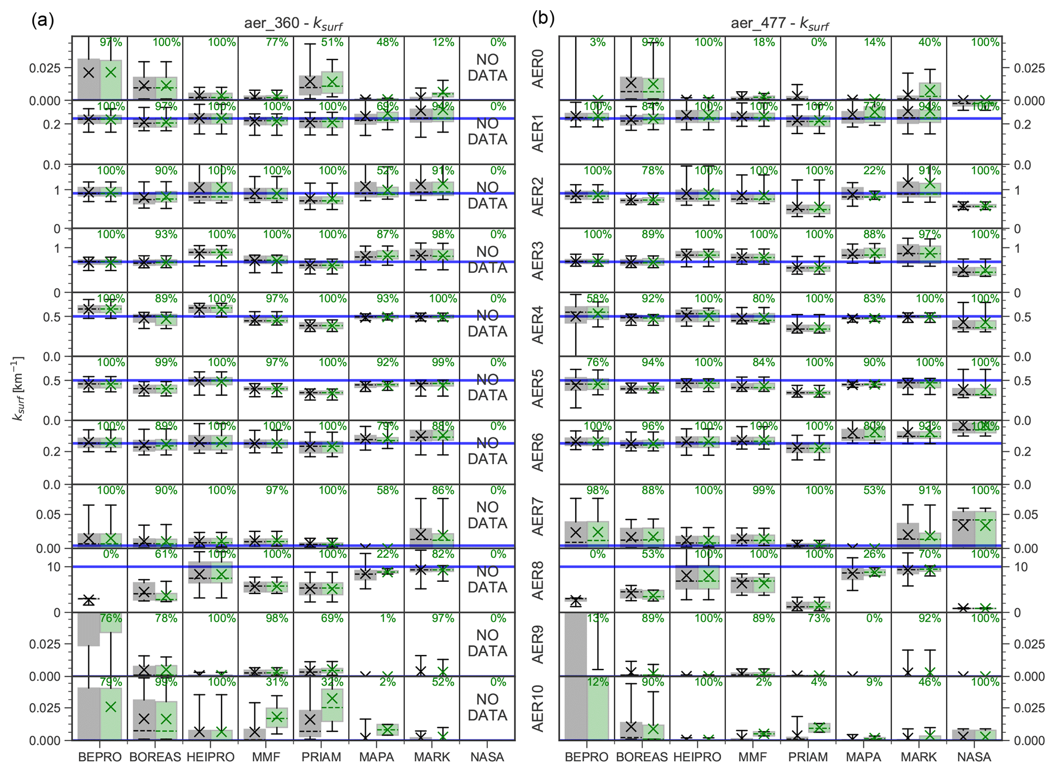
Figure 19Box–whisker plots of the retrieved surface aerosol extinction at 360 nm (a) and 477 nm (b) for the different aerosol scenarios (rows) and retrieval algorithms (columns) based on retrievals using noisy dSCDs. Crosses show the mean, and dashed horizontal lines show the median. Shaded areas indicate the (25 %–75 %) percentile, and whiskers show the (5 %–95 %) percentile. The true AOT is shown as the blue horizontal line. For each algorithm, all data are shown on the left in black, and data marked as valid are on the right in green. Also shown is the percentage of valid data.
As a result of a poor convergence of modelled and measured dSCDs (see Sect. 6.3), bePRO fails to retrieve the extinction profile at 477 nm for aerosol-free atmospheres (AER0) and for a high-lying cloud (AER10). The RMS difference between true and retrieved extinction is significantly higher for bePRO than for other algorithms for AER4 (100 m thick aerosol layer). As a result of these instabilities, the linear regression of retrieved and true aerosol extinction coefficients at 477 nm yields a smaller slope (0.76) and regression coefficient (0.26) for bePRO than for the other algorithms when including all data. After filtering out ≈75 % of data flagged as invalid, the accuracy of the bePRO results is similar to the other algorithms.
PRIAM and NASA underestimate the aerosol extinction at 477 nm with slopes of only 0.72 and 0.63, respectively. Furthermore, PRIAM falsely retrieves a non-existing uplifted aerosol layer around 1 km in altitude with a peak extinction >0.1 km−1 for aerosol-free atmospheres (AER0 and AER10) at 477 nm, whereas MAPA retrieves elevated aerosol extinction at the top of the retrieval domain between 3.5 and 4 km for these scenarios at both 360 and 477 nm. This is a consequence of the fact that there are no a priori constraints on extinction profiles made in MAPA, and the resulting dSCDs are almost unaffected by high cloud layers. Most of the MAPA profiles for the AER10 scenario are, however, flagged as invalid, leaving only 2 % of valid profiles (see Figs. S1 and S2).
The retrieval is generally more stable for trace gases (Figs. 13 and 14) than for aerosols. Obviously, it is sufficient to constrain the trace gas retrieval with an aerosol profile that realistically reproduces the light path, even if the extinction profile differs from the truth. Furthermore, trace gas retrievals are probably more stable because they constitute a linear problem in contrast to the non-linear aerosol retrieval.
With the exception of NO2 from bePRO, the algorithms reproduce exponential trace gas profiles (TG1, TG2, and TG3) well, with little bias towards the a priori at high altitudes (Figs. 13 and 14). As for aerosols at 477 nm, bePRO NO2 profiles suffer from significant instabilities, and BOREAS shows oscillating features with negative values for altitudes between 1 and 2 km. These discrepancies of the bePRO and BOREAS results are probably due to the fact that they operate in linear space. The vertical extent and trace gas concentration of the shallow trace gas layers TG4 and TG5 are well reproduced by all algorithms except NASA. HEIPRO NO2 results for TG4 suffer from outliers for the AER9 scenario, where NO2 above the cloud is overestimated. As for aerosols, the degree of smoothing of the 1 km box profile (TG6) is higher for the OEM than for the parametrised algorithms. The peak altitude of the uplifted profile (TG7) at 360 nm is underestimated by all algorithms except MAPA and MARK, with the latter overestimating the altitude of the trace gas layer. The agreement between retrieved and true TG7 profiles is better for NO2, where HEIPRO, MMF, and MAPA retrieve the peak altitude at the right location, than for HCHO. This is probably owing to the lower information content and lower sensitivity for high altitudes in the UV range compared to the visible range (see Sect. 6.2). The uplifted trace gas profile (TG7) is subject to a larger degree of smoothing than the corresponding uplifted aerosol profile (AER7). Owing to the limited vertical resolution of MAX-DOAS measurements, the fine structure of the trace gas profiles measured by a NO2 balloon sonde (TG8 and TG9) is not well reproduced by the retrievals. The lowest level of agreement between true and retrieved trace gas profiles is found for the fog scenario (AER8) since the high extinction at the ground leads to a very small information content and a low sensitivity for trace gases except for the lowermost atmospheric layers (see Sect. 6.2).
MAPA, MARK, and NASA algorithms retrieve profiles close to zero for the trace gas free atmospheres (TG0), whereas the OEM algorithms either exhibit a slight bias towards the a priori (HEIPRO, MMF, PRIAM) or oscillate around zero (bePRO, BOREAS) for this scenario. Sensitivity studies based on the MMF algorithm have shown that these oscillations are suppressed if the logarithm of the profile is retrieved, as is the case for HEIPRO, MMF, and PRIAM. This representation also prevents the retrieval of negative values, which occur for bePRO and BOREAS, in particular for TG0 and TG4.
Except for bePRO NO2, a linear regression between true and retrieved trace gas concentrations yields slopes between 0.9 and 1.08 (see Fig. 15). Regression coefficients usually exceed 0.8, except for NO2 in the case of bePRO (R=0.36), BOREAS (R=0.75), PRIAM (R=0.72), and MARK (R=0.77). In particular at 360 nm, MMF and MARK aerosols appear to be more sensitive to noise than the other algorithms, with Pearson's R decreasing from 0.93 to 0.76 (MMF) and from 0.84 to 0.77 (MARK) after adding noise to the synthetic measurements. In general, NO2 profiles from the OEM algorithms appear to be more sensitive to measurement noise than HCHO profiles.

Figure 20Same as Fig. 19, but for HCHO (a) and NO2 (b) surface concentrations. The median for each aerosol scenario is shown as coloured symbol as indicated in the legend.
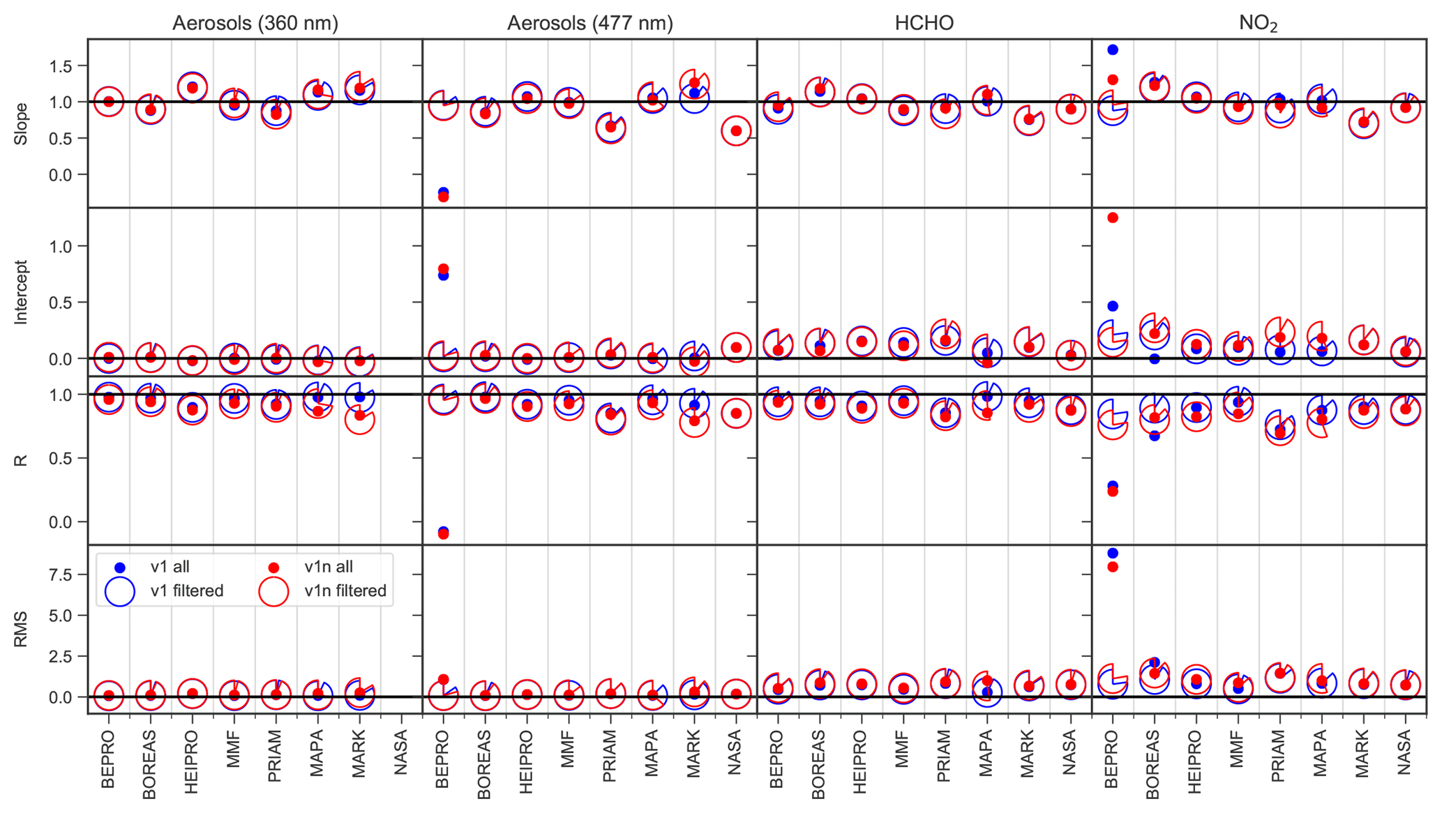
Figure 21Slope, intercept, regression coefficient, and RMS for the correlation between true and retrieved aerosol extinction as well as HCHO and NO2 surface concentration. Intercept and RMS values are in dimensionless units for aerosols and 1011 molec cm−3 for HCHO and NO2. Cloud and fog scenarios (AER8, AER9, AER10) are excluded from the regression analysis.
6.5 Comparison of total columns
In this section, the ability of the retrieval algorithms to retrieve aerosol and trace gas total columns is discussed. Box–whisker plots comparing retrieved and true AOT at 360 and 477 nm are shown in Fig. 16. The corresponding plots for HCHO and NO2 VCDs are shown in Fig. 17. The parameters of a linear regression between retrieved and true total columns are shown in Fig. 18. Note that the total column is defined here as the integral of extinction coefficient and number concentration within the retrieval domain, i.e. from the surface to 4 km in altitude. This means that, for example, a high-altitude cloud above the retrieval domain as in the AER10 scenario is not considered in the calculation of the AOT.
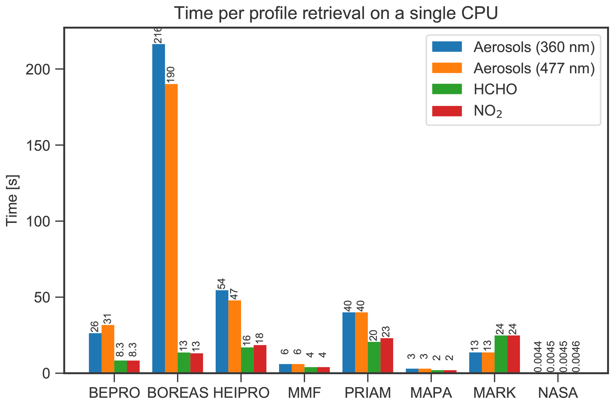
Figure 22Time in seconds for the retrieval of a single profile on a single CPU core for each participant, separated by the target species as denoted in the legend.
The total column of both trace gases and aerosols is retrieved accurately by most algorithms. Except for foggy conditions (AER8), there is little dependency of the accuracy of the retrieved trace gas VCD on the aerosol profile. As expected from the limited sensitivity to high altitudes, the total columns from OEM algorithms tend to be biased towards the a priori. For the aerosol and trace gas free scenarios AER0 and TG0, a positive bias of (0.02–0.06) for AOT and (0.2–0.35)×1016 molec cm−2 for trace gases is found for the OEM algorithms. Ranging from 0.05 to 0.15, the AOT bias is somewhat higher for AER10 with a cloud above 5 km in altitude than for AER0. The OEM algorithms show a negative bias for the high-extinction scenario AER2 (AOT of 1) and a positive bias for the shallow layers AER4, AER5, and TG4, TG5. The bias towards the a priori is furthermore reflected by a smaller slope of the linear regression between retrieved and true total column for the OEM algorithms compared to the parametrised and analytical algorithms MAPA, MARK, and NASA for all species except NO2 (see Fig. 18). Again, bePRO shows poor performance in the visible range with regression coefficients of 0.02 and 0.71 for aerosols at 477 nm and NO2, respectively, while all other algorithms yield R>0.85 and R>0.93 for aerosols and trace gases, respectively. These discrepancies mainly occur for the AER0 scenario, and to a lesser extent also for AER4.
The parametrised algorithms MAPA and MARK accurately retrieve the total column in most cases. Exceptions are the AER6 and AER7 scenarios (1 km box profile and uplifted profile), where both algorithms show a positive bias. Both MAPA and MARK show a significant scatter of the AOT for AER0, AER1, AER2, AER7, and AER10 that, in the case of MAPA, is reduced by filtering out a significant fraction of the data (28 % at 360 nm and 37 % at 477 nm). Furthermore, MAPA significantly overestimates the AOT at 477 nm with a slope of 1.4, and yields a regression coefficient of only 0.56 for the AOT at 360 nm when considering all data. Regression parameters for MAPA are, however, comparable to those from the other algorithms after removing data flagged as invalid. MARK flags almost all TG0 data as invalid, although the agreement between true and retrieved VCD is very good for this algorithm. The NASA algorithm retrieves the HCHO and NO2 VCD accurately, but shows a significant negative bias for all aerosol scenarios at 477 nm (except for AER6), where the regression coefficient is less than 0.6.
6.6 Comparison of surface values
In this section, the agreement between true and retrieved surface extinction and surface concentration (i.e. the values in the lowermost layer of the respective profiles with a thickness of 200 m) are discussed. As for the total column discussed in the previous section, Figs. 19 and 20 show box–whisker plots for the aerosol and trace gas surface values, and Fig. 21 lists the parameters of the linear regression between true and retrieved aerosol extinction and trace gas concentration in the lowermost retrieval layer.
Surface aerosol extinction and trace gas profiles are generally well reproduced. For bePRO retrievals in the visible, however, a negative slope and no significant correlation () between true and retrieved values are found for surface aerosol extinction at 477 nm. Furthermore, the regression coefficient for bePRO NO2 is only 0.24 due to the aforementioned deviations in case of the AER0 and AER4 scenarios. However, the regression parameters of the bePRO algorithm significantly improve after discarding about 20 % of the profiles marked as invalid. The OEM algorithms yield a small positive bias for scenarios with no or only small surface extinction coefficients and trace gas concentrations (AER0, AER7, AER9, AER10, TG0, and TG7). PRIAM and NASA both underestimate the aerosol extinction at 477 nm (slope between 0.6 and 0.65). In contrast, HEIPRO, MAPA, and MARK overestimate the surface extinction, in particular at 360 nm (slope >1.16), and yield smaller regression coefficients (R<0.9 at 360 nm) than the other algorithms.
For the prescribed profile scenarios, retrieved aerosol surface extinction (mean regression coefficient from all algorithms at 360 nm and at 477 nm) shows a better agreement with the true value than the AOT ( at 360 nm and at 477 nm). The opposite is true for trace gases, where the agreement of the total column ( and for HCHO and NO2, respectively) is better than for the surface mixing ratio ( and ).
6.7 Computational performance
In order to assess the numerical performance of the different retrieval algorithms, the duration for a single profile retrieval was reported by each participant. For multiprocessor systems, the total time has been multiplied by the number of processor kernels used for the retrieval. It is important to note that the retrievals were performed individually by each participant, using computers with different performances. A more accurate comparison would require to run all algorithms on the same computer, which is outside the scope of this study. The results of the benchmark test are shown in Fig. 22.
The OEM algorithms, which rely on online radiative transfer calculations, require between 4 (MMF) and 23 s (PRIAM) for the retrieval of a single trace gas profile. The duration for the retrieval of an aerosol profile ranges between 6 s for MMF and more than 3.5 min for BOREAS. The large range of computational effort for aerosols probably results from the different approaches for the calculation of the weighting functions. The BOREAS aerosol retrieval relies on radiative transfer simulations at several wavelengths, resulting in the lowest computational performance, followed by HEIPRO, whose aerosol weighting function calculation is based on the finite difference method, leading to about 1 min for an aerosol retrieval, while MMF and bePRO are significantly faster since they rely on analytically calculated aerosol weighting functions.
The parametrised algorithms MAPA and MARK show significant differences in computational performance, although both rely on LUTs for the weighting functions. MARK requires 13 and 24 s for aerosol and trace gas retrievals, respectively, while MAPA aerosol and trace gas retrievals are executed within 3 and 2 s, respectively.
The NASA algorithm, which does not rely on radiative transfer modelling but on an analytical approach, is outstanding in terms of computational performance. The retrieval of a single aerosol or trace gas profile requires less than 5 ms, and is thus almost 3 orders of magnitude faster than the second fastest algorithm, MAPA.
Eight different algorithms for the retrieval of aerosol and trace gas vertical profiles from MAX-DOAS measurements have been compared under a large variety of atmospheric conditions by using synthetic measurements. Both OEM and parametrised algorithms, and also the analytic approach by NASA, show equally good performance in terms of the reproduction of the true atmospheric state, with a typical accuracy (in terms of RMS difference between true and retrieved state) of (0.08–0.25) km−1 for surface aerosol extinction and (5.9–15.0) ×1010 molec cm−3 (or about 2.4–6 ppb) for HCHO and NO2 surface concentrations. These deviations, and also a potential positive bias towards the a priori for OEM algorithms, can be quite significant for clean air conditions, but are relatively small in polluted areas where several tens of parts per billion of NO2 and HCHO and aerosol extinction of up to 5 km−1 can be present (e.g. Vlemmix et al., 2015b). Total columns of trace gases can be retrieved with a higher accuracy than for aerosols, with slopes >0.85 and correlation coefficients >0.95 in most cases. However, the accuracy is expected to be higher for real atmospheric measurements (e.g. Irie et al., 2011) since some of the scenarios within this study are quite arbitrary with the intention to test the algorithms under extreme conditions.
There are only a few exceptions from this high level of agreement between the retrieved atmospheric state from the different algorithms. As a result of lack of convergence between true and modelled slant column densities, bePRO profiles are subject to a high degree of instability in the visible wavelength range for the aerosol scenarios AER0, AER8, AER9, and AER10 and to a lesser extent also AER4. Up to 25 % of the bePRO profiles need to be discarded in order to achieve an accuracy similar to the other algorithms. However, bePRO performs well when convergence is reached. The synthetic data used for the study are not necessarily representative of real measurements, especially in terms of dSCDs errors, and sensitivity tests performed by increasing the dSCDs errors but also previous publications (e.g. Hendrick et al., 2014; Vlemmix et al., 2015b) have shown that bePRO performs generally well with real measurement data, also in terms of convergence.
Aerosol AVKs from BOREAS differ from those of other OEM retrievals as additional regularisation is applied. They can therefore not be compared to those from the other retrievals and also do not comply with Eq. (6). About 54 % of the data from MAPA are flagged as invalid (39 % of the moderate scenarios AER1–AER7, and 93 % of the cloud/fog scenarios AER8–AER10), although the level of agreement of all MAPA profiles with the truth is comparable to the other algorithms, indicating that the MAPA flagging criteria might be too strict. However, the MAPA flagging successfully removes almost all outliers.
OEM algorithms tend to produce profiles biased towards the a priori, in particular at high altitudes where the sensitivity to the atmospheric state is small. OEM algorithms retrieving the logarithm of the target parameters show a higher degree of stability with fewer oscillations than those operating in linear space. Parametrised algorithms do not suffer from this disadvantage, but the possible results can be wide-spread when the sensitivity to the atmospheric state is low, which is particularly the case at high altitude or above layers with high extinction. However, despite these conceptual differences, the overall accuracy of OEM and parametrised algorithms is very similar.
Based on an analytical approach without using RTM calculations, the NASA algorithm is by far the fastest, with the retrieval of a single profile requiring less than 5 µs, followed by MAPA as the second fastest algorithm, requiring 2–3 s for a single retrieval based on LUTs. Involving online radiative transfer calculations, most OEM algorithms are slower, but their computational performance covers a wide range, mainly owing to the different approaches for the calculation of weighting functions. Being only about 2–3 times slower than the parametrised MAPA algorithm, MMF is by far the fastest OEM algorithm.
In summary, it can be concluded that, with only a few exceptions, the algorithms presented here are capable of realistically retrieving aerosol and trace gas profiles in the lowermost ≈2 km of the atmosphere, yielding 1.5–3.5 independent pieces of information depending on the target species and the atmospheric conditions. The comparison using synthetic measurements of course represents an idealisation in many respects, and the agreement between true and retrieved state might be worse for true atmospheric measurements. In particular, it has been assumed that forward model parameters, such as surface albedo, aerosol optical properties, etc., are perfectly well known, which is usually not the case for ambient measurements. Furthermore, the atmosphere has been assumed to be horizontally homogeneous, while in reality inhomogeneities, in particular broken clouds, can have a significant influence on MAX-DOAS measurements. Also, several instrumental aspects, such as a finite instrumental field of view, instrumental stray light, pointing inaccuracies, or difficulties when pointing the telescope closely towards the Sun, were not considered here. Furthermore, the idealised set of atmospheric states considered in this synthetic intercomparison exercise does not cover all atmospheric conditions.
As a result of this study, the MMF and the MAPA algorithms, both showing best performance in terms of reconstruction of the atmospheric state and computational speed, were selected as profile algorithms for the FRM4DOAS centralised near-real-time algorithm for a harmonised processing of MAX-DOAS data, which are planned to be made available to the community in the near future.
A detailed comparison of vertical profiles of trace gases and aerosols from MAX-DOAS field measurements performed during the CINDI-2 (http://www.tropomi.eu/data-products/cindi-2) campaign with co-located independent measurements, which comprises retrievals from nine algorithms and 16 workgroups, will be the subject of a companion publication.
The bePRO and HEIPRO algorithms are available from the authors upon request (Francois Hendrick, francois.hendrick@aeronomie.be, and Udo Frieß, udo.friess@iup.uni-heidelberg.de).
The reference database of synthetic dSCDs is available on the FRM4DOAS web page (http://frm4doas.aeronomie.be/index.php/documents, Frieß et al., 2019).
The supplement related to this article is available online at: https://doi.org/10.5194/amt-12-2155-2019-supplement.
The intercomparison strategy and retrieval settings were developed by FH and UF. Forward modelling of dSCDs and retrieval of vertical profiles was performed by UF, SB, LAB, TB, MMF, FH, AP, AR, MvR, ES, TV, TW, and YW. The visualisation of the data was performed by UF and J-LT. UF performed the statistical analysis of the data. VVR developed the SCIATRAN radiative transfer model.
The authors declare that they have no conflict of interest.
The funding of this study by the FRM4DOAS project (ESA contract no. 4000118181/16/I-EF) is gratefully acknowledged. The activities of the IUP Heidelberg were supported by the DFG project RAPSODI (grant no. PL 193/17-1). We are also thankful to Marc Allaart (KNMI) for providing the ozone-sonde data from De Bilt for constructing the temperature and pressure profiles used as input for the RT modelling.
This paper was edited by Andreas Hofzumahaus and reviewed by three anonymous referees.
Beirle, S., Dörner, S., Donner, S., Remmers, J., Wang, Y., and Wagner, T.: The Mainz profile algorithm (MAPA), Atmos. Meas. Tech., 12, 1785–1806, https://doi.org/10.5194/amt-12-1785-2019, 2019. a, b, c
Bösch, T., Rozanov, V., Richter, A., Peters, E., Rozanov, A., Wittrock, F., Merlaud, A., Lampel, J., Schmitt, S., de Haij, M., Berkhout, S., Henzing, B., Apituley, A., den Hoed, M., Vonk, J., Tiefengraber, M., Müller, M., and Burrows, J. P.: BOREAS – a new MAX-DOAS profile retrieval algorithm for aerosols and trace gases, Atmos. Meas. Tech., 11, 6833–6859, https://doi.org/10.5194/amt-11-6833-2018, 2018. a, b
Clémer, K., Van Roozendael, M., Fayt, C., Hendrick, F., Hermans, C., Pinardi, G., Spurr, R., Wang, P., and De Mazière, M.: Multiple wavelength retrieval of tropospheric aerosol optical properties from MAXDOAS measurements in Beijing, Atmos. Meas. Tech., 3, 863–878, https://doi.org/10.5194/amt-3-863-2010, 2010 a, b, c
de Haan, J. F., Bosma, P. B., and Hovenier, J. W.: The adding method for multiple scattering calculations of polarized light, Astron. Astrophys., 183, 371–391, 1987. a
Deutschmann, T., Beirle, S., Frieß, U., Grzegorski, M., Kern, C., Kritten, L., Platt, U., Prados-Roman, C., Puķīte, J., Wagner, T., Werner, B., and Pfeilsticker, K.: The Monte Carlo atmospheric radiative transfer model McArtim: Introduction and validation of Jacobians and 3D features, J. Quant. Spectrosc. Ra., 112, 1119–1137, https://doi.org/10.1016/j.jqsrt.2010.12.009, 2011. a
Friedrich, M. M., Rivera, C., Stremme, W., Ojeda, Z., Arellano, J., Bezanilla, A., García-Reynoso, J. A., and Grutter, M.: NO2 vertical profiles and column densities from MAX-DOAS measurements in Mexico City, Atmos. Meas. Tech. Discuss., https://doi.org/10.5194/amt-2018-358, in review, 2018. a
Frieß, U., Monks, P., Remedios, J., Rozanov, A., Sinreich, R., Wagner, T., and Platt, U.: MAX-DOAS O4 measurements: A new technique to derive information on atmospheric aerosols: 2. Modeling studies, J. Geophys. Res., 111, D14203, https://doi.org/10.1029/2005JD006618, 2006. a, b, c
Frieß, U., Sihler, H., Sander, R., Pöhler, D., Yilmaz, S., and Platt, U.: The vertical distribution of BrO and aerosols in the Arctic: Measurements by active and passive differential optical absorption spectroscopy, J. Geophys. Res., 116, D00R04, https://doi.org/10.1029/2011JD015938, 2011. a
Frieß, U., Klein Baltink, H., Beirle, S., Clémer, K., Hendrick, F., Henzing, B., Irie, H., de Leeuw, G., Li, A., Moerman, M. M., van Roozendael, M., Shaiganfar, R., Wagner, T., Wang, Y., Xie, P., Yilmaz, S., and Zieger, P.: Intercomparison of aerosol extinction profiles retrieved from MAX-DOAS measurements, Atmos. Meas. Tech., 9, 3205–3222, https://doi.org/10.5194/amt-9-3205-2016, 2016. a
Frieß, U., Beirle, S., Alvarado Bonilla, L., Bösch, T., Friedrich, M. M., Hendrick, F., Piters, A., Richter, A., van Roozendael, M., Rozanov, V. V., Spinei, E., Tirpitz, J.-L., Vlemmix, T., Wagner, T., and Wang, Y.: The FRM4DOAS MAX-DOAS synthetic dSCD database for profile retrieval intercomparisons, available at: http://frm4doas.aeronomie.be/index.php/documents, last access: 8 April 2019. a
Hartl, A. and Wenig, M. O.: Regularisation model study for the least-squares retrieval of aerosol extinction time series from UV/VIS MAX-DOAS observations for a ground layer profile parameterisation, Atmos. Meas. Tech., 6, 1959–1980, https://doi.org/10.5194/amt-6-1959-2013, 2013. a
Hay, T.: MAX-DOAS measurements of bromine explosion events in McMurdo Sound, Antarctica, PhD thesis, University of Canterbury, 2010. a
Heckel, A., Richter, A., Tarsu, T., Wittrock, F., Hak, C., Pundt, I., Junkermann, W., and Burrows, J. P.: MAX-DOAS measurements of formaldehyde in the Po-Valley, Atmos. Chem. Phys., 5, 909–918, https://doi.org/10.5194/acp-5-909-2005, 2005. a
Hendrick, F., Müller, J.-F., Clémer, K., Wang, P., De Mazière, M., Fayt, C., Gielen, C., Hermans, C., Ma, J. Z., Pinardi, G., Stavrakou, T., Vlemmix, T., and Van Roozendael, M.: Four years of ground-based MAX-DOAS observations of HONO and NO2 in the Beijing area, Atmos. Chem. Phys., 14, 765–781, https://doi.org/10.5194/acp-14-765-2014, 2014. a
Henyey, L. C. and Greenstein, J. L.: Diffuse radiation in the Galaxy, Astrophys. J., 93, 70–83, 1941. a
Holla, R.: Reactive Halogen Species above Salt Lakes and Salt Pans, PhD thesis, University of Heidelberg, 2013. a
Hönninger, G., von Friedeburg, C., and Platt, U.: Multi axis differential optical absorption spectroscopy (MAX-DOAS), Atmos. Chem. Phys., 4, 231–254, https://doi.org/10.5194/acp-4-231-2004, 2004. a
Irie, H., Kanaya, Y., Akimoto, H., Iwabuchi, H., Shimizu, A., and Aoki, K.: First retrieval of tropospheric aerosol profiles using MAX-DOAS and comparison with lidar and sky radiometer measurements, Atmos. Chem. Phys., 8, 341–350, https://doi.org/10.5194/acp-8-341-2008, 2008. a
Irie, H., Takashima, H., Kanaya, Y., Boersma, K. F., Gast, L., Wittrock, F., Brunner, D., Zhou, Y., and Van Roozendael, M.: Eight-component retrievals from ground-based MAX-DOAS observations, Atmos. Meas. Tech., 4, 1027–1044, https://doi.org/10.5194/amt-4-1027-2011, 2011. a
Kreher, K., Van Roozendael, M., Hendrick, F., Apituley, A., Dimitropoulou, E., Frieß, U., Richter, A., Wagner, T., Abuhassan, N., Ang, L., Anguas, M., Bais, A., Benavent, N., Bösch, T., Bognar, K., Borovski, A., Bruchkovsky, I., Cede, A., Chan, K. L., Donner, S., Drosoglou, T., Fayt, C., Finkenzeller, H., Garcia-Nieto, D., Gielen, C., Gómez-Martín, L., Hao, N., Hermans, C., Hoque, S., Irie, H., Jin, J., Johnston, P., Khayyam Butt, J., Khokhar, F., Koenig, T. K., Kuhn, J., Kumar, V., Lampel, J., Liu, C., Ma, J., Merlaud, A., Mishra, A. K., Müller, M., Navarro-Comas, M., Ostendorf, M., Pazmino, A., Peters, E., Pinardi, G., Pinharanda, M., Piters, A., Platt, U., Postylyakov, O., Prados-Roman, C., Puentedura, O., Querel, R., Saiz-Lopez, A., Sinha, V., Schönhardt, A., Seyler, A., Schreier, S. F., Seyler, A., Spinei, E., Strong, K., Tack, F., Tiefengraber, M., Tirpitz, J.-L., van Gent, J., Volkamer, R., Vrekoussis, M., Wang, S., Wang, Z., Wenig, M., Wittrock, F., Xie, P., Xu, J., Yela, M., Zhang, C., and Zhao, X.: Intercomparison of NO2, O4, O3 and HCHO slant column measurements by MAX-DOAS and zenith-sky UV-Visible spectrometers, Atmos. Meas. Tech., in preparation, 2019. a, b
Levenberg, K.: A method for the solution of certain non-linear problems in least squares, Q. Appl., Math., 2, 164–168, 1944. a
Marquardt, D. W.: An Algorithm for Least-Squares Estimation of Nonlinear Parameters, J. Soc. Ind. App. Math., 11, 431–441, 1963. a
Meller, R. and Moortgat, G. K.: Temperature dependence of the absorption cross sections of formaldehyde between 223 and 323 K in the wavelength range 225-375 nm, J. Geophys. Res.-Atmos., 105, 7089–7101, https://doi.org/10.1029/1999JD901074, 2000. a
Ortega, I., Berg, L. K., Ferrare, R. A., Hair, J. W., Hostetler, C. A., and Volkamer, R.: Elevated aerosol layers modify the O2 absorption measured by ground-based MAX-DOAS, J. Quant. Spectrosc. Ra., 176, 34–49, https://doi.org/10.1016/j.jqsrt.2016.02.021, 2016. a
Platt, U. and Stutz, J.: Differential optical absorption spectroscopy, Springer Verlag, 2008. a
Rodgers, C. D.: Inverse methods for atmospheric sounding, theory and practice, Series on Atmospheric, Oceanic and Planetary Physics, World Scientific, 2000. a, b, c, d, e
Rozanov, A., Bovensmann, H., Bracher, A., Hrechanyy, S., Rozanov, V., Sinnhuber, M., Stroh, F., and Burrows, J.: NO2 and BrO vertical profile retrieval from SCIAMACHY limb measurements: Sensitivity studies, Adv. Space Res., 36, 846–854, https://doi.org/10.1016/j.asr.2005.03.013, 2005. a
Rozanov, V., Rozanov, A., Kokhanovsky, A., and Burrows, J.: Radiative transfer through terrestrial atmosphere and ocean: Software package {SCIATRAN}, J. Quant. Spectrosc. Ra., 133, 13–71, https://doi.org/10.1016/j.jqsrt.2013.07.004, 2014. a, b
Sinreich, R., Merten, A., Molina, L., and Volkamer, R.: Parameterizing radiative transfer to convert MAX-DOAS dSCDs into near-surface box-averaged mixing ratios, Atmos. Meas. Tech., 6, 1521–1532, https://doi.org/10.5194/amt-6-1521-2013, 2013. a
Spinei et al.: Fast aerosol extinction coefficient profile estimation from MAXDOAS UV/VIS measurements, in preparation, 2019. a
Spurr, R.: LIDORT and VLIDORT: Linearized pseudo-spherical scalar and vector discrete ordinate radiative transfer models for use in remote sensing retrieval problems, in: Light Scattering Reviews 3, edited by: Kokhanovsky, A., Springer Praxis Books, Springer Berlin Heidelberg, 229–275, https://doi.org/10.1007/978-3-540-48546-9_7, 2008. a
Spurr, R., de Haan, J., van Oss, R., and Vasilkov, A.: Discrete-ordinate radiative transfer in a stratified medium with first-order rotational Raman scattering, J. Quant. Spectrosc. Ra., 109, 404–425, https://doi.org/10.1016/j.jqsrt.2007.08.011, 2008. a, b
Spurr, R. J.: VLIDORT: A linearized pseudo-spherical vector discrete ordinate radiative transfer code for forward model and retrieval studies in multilayer multiple scattering media, J. Quant. Spectrosc. Ra., 102, 316–342, https://doi.org/10.1016/j.jqsrt.2006.05.005, 2006. a
Stammes, P., de Haan, J. F., and Hovenier, J. W.: The polarized internal radiation field of a planetary atmosphere, Astron. Astrophys., 225, 239–259, 1989. a
Thalman, R. and Volkamer, R.: Temperature dependent absorption cross-sections of O2−O2 collision pairs between 340 and 630 nm and at atmospherically relevant pressure, Phys. Chem. Chem. Phys., 15, 15371–15381, https://doi.org/10.1039/C3CP50968K, 2013. a
Vandaele, A. C., Hermans, C., Simon, P. C., Carleer, M., Colin, R., Fally, S., Mérienne, M. F., Jenouvrier, A., and Coquart, B.: Measurements of the NO2 absorption cross-section from 42 000 cm−1 to 10 000 cm−1 (238–1000 nm) at 220 K and 294 K, J. Quant. Spectrosc. Ra., 59, 171–184, https://doi.org/10.1016/S0022-4073(97)00168-4, 1998. a
Vlemmix, T., Piters, A. J. M., Berkhout, A. J. C., Gast, L. F. L., Wang, P., and Levelt, P. F.: Ability of the MAX-DOAS method to derive profile information for NO2: can the boundary layer and free troposphere be separated?, Atmos. Meas. Tech., 4, 2659–2684, https://doi.org/10.5194/amt-4-2659-2011, 2011. a, b
Vlemmix, T., Eskes, H. J., Piters, A. J. M., Schaap, M., Sauter, F. J., Kelder, H., and Levelt, P. F.: MAX-DOAS tropospheric nitrogen dioxide column measurements compared with the Lotos-Euros air quality model, Atmos. Chem. Phys., 15, 1313–1330, https://doi.org/10.5194/acp-15-1313-2015, 2015a. a
Vlemmix, T., Hendrick, F., Pinardi, G., De Smedt, I., Fayt, C., Hermans, C., Piters, A., Wang, P., Levelt, P., and Van Roozendael, M.: MAX-DOAS observations of aerosols, formaldehyde and nitrogen dioxide in the Beijing area: comparison of two profile retrieval approaches, Atmos. Meas. Tech., 8, 941–963, https://doi.org/10.5194/amt-8-941-2015, 2015b. a, b, c, d
Wagner, T., Dix, B., von Friedeburg, C., Frieß, U., Sanghavi, S., Sinreich, R., and Platt, U.: MAX-DOAS O4 measurements: A new technique to derive information on atmospheric aerosols – principles and information content, J. Geophys. Res., 109, D22205, https://doi.org/10.1029/2004JD004904, 2004. a, b
Wagner, T., Burrows, J. P., Deutschmann, T., Dix, B., von Friedeburg, C., Frieß, U., Hendrick, F., Heue, K.-P., Irie, H., Iwabuchi, H., Kanaya, Y., Keller, J., McLinden, C. A., Oetjen, H., Palazzi, E., Petritoli, A., Platt, U., Postylyakov, O., Pukite, J., Richter, A., van Roozendael, M., Rozanov, A., Rozanov, V., Sinreich, R., Sanghavi, S., and Wittrock, F.: Comparison of box-air-mass-factors and radiances for Multiple-Axis Differential Optical Absorption Spectroscopy (MAX-DOAS) geometries calculated from different UV/visible radiative transfer models, Atmos. Chem. Phys., 7, 1809–1833, https://doi.org/10.5194/acp-7-1809-2007, 2007. a
Wagner, T., Beirle, S., Brauers, T., Deutschmann, T., Frieß, U., Hak, C., Halla, J. D., Heue, K. P., Junkermann, W., Li, X., Platt, U., and Pundt-Gruber, I.: Inversion of tropospheric profiles of aerosol extinction and HCHO and NO2 mixing ratios from MAX-DOAS observations in Milano during the summer of 2003 and comparison with independent data sets, Atmos. Meas. Tech., 4, 2685–2715, https://doi.org/10.5194/amt-4-2685-2011, 2011. a, b
Wang, Y., Li, A., Xi, P.-H., Chen, H., Xu, J., Wu, F.-C., Liu, J.-G., and Liu, W.-Q.: Retrieving vertical profile of aerosol extinction by multi-axis differential optical absorption spectroscopy, Acta Phys. Sin., 62, 180705, https://doi.org/10.7498/aps.62.180705, 2013. a
Yilmaz, S.: Retrieval of Atmospheric Aerosol and Trace Gas Vertical Profiles using Multi-Axis Differential Optical Absorption Spectroscopy, PhD thesis, University of Heidelberg, 2012. a
Zielcke, J.: Observations of reactive bromine, iodine and chlorine species in the Arctic and Antarctic with Differential Optical Absorption Spectroscopy, PhD thesis, https://doi.org/10.11588/heidok.00018932, 2015. a
- Abstract
- Introduction
- Profile retrieval and intercomparison strategy
- Retrieval algorithms
- Model scenarios and RTM settings
- Intercomparison of forward modelled SCDs
- Retrieval algorithm comparison
- Conclusions
- Code availability
- Data availability
- Author contributions
- Competing interests
- Acknowledgements
- Review statement
- References
- Supplement