the Creative Commons Attribution 4.0 License.
the Creative Commons Attribution 4.0 License.
 | 12 Apr 2019
Analysis of functional groups in atmospheric aerosols by infrared spectroscopy: systematic intercomparison of calibration methods for US measurement network samples
Matteo Reggente
Ann M. Dillner
Satoshi Takahama
Peak fitting (PF) and partial least squares (PLS) regression have been independently developed for estimation of functional groups (FGs) from Fourier transform infrared (FTIR) spectra of ambient aerosol collected on Teflon filters. PF is a model that quantifies the functional group composition of the ambient samples by fitting individual Gaussian line shapes to the aerosol spectra. PLS is a data-driven, statistical model calibrated to laboratory standards of relevant compounds and then extrapolated to ambient spectra. In this work, we compare the FG quantification using the most widely used implementations of PF and PLS, including their model parameters, and also perform a comparison when the underlying laboratory standards and spectral processing are harmonized. We evaluate the quantification of organic FGs (alcohol COH, carboxylic COOH, alkane CH, carbonyl CO) and ammonium, using external measurements (organic carbon (OC) measured by thermal optical reflectance (TOR) and ammonium by balance of sulfate and nitrate measured by ion chromatography). We evaluate our predictions using 794 samples collected in the Interagency Monitoring of PROtected Visual Environments (IMPROVE) network (USA) in 2011 and 238 laboratory standards from Ruthenburg et al. (2014) (available at https://doi.org/10.1016/j.atmosenv.2013.12.034). Each model shows different biases. Overall, estimates of OC by FTIR show high correlation with TOR OC. However, PLS applied to unprocessed (raw spectra) appears to underpredict oxygenated functional groups in rural samples, while other models appear to underestimate aliphatic CH bonds and OC in urban samples. It is possible to adjust model parameters (absorption coefficients for PF and number of latent variables for PLS) within limits consistent with calibration data to reduce these biases, but this analysis reveals that further progress in parameter selection is required. In addition, we find that the influence of scattering and anomalous transmittance of infrared in coarse particle samples can lead to predictions of OC by FTIR which are inconsistent with TOR OC. We also find through several means that most of the quantified carbonyl is likely associated with carboxylic groups rather than ketones or esters. In evaluating state-of-the-art methods for FG abundance by FTIR, we suggest directions for future research.
- Article
(5472 KB) - Companion paper
-
Supplement
(1926 KB) - BibTeX
- EndNote


Atmospheric aerosol, also called particulate matter (PM), is made up of organic compounds, inorganic salts, trace elements, black carbon, and water, among other substances. Accounting for its total mass in terms of its speciated composition is desirable for regulatory and epidemiological reasons, and this goal poses a substantial challenge for environmental analytical measurement. Organic compounds in particular can contribute 20 %–80 % of the atmospheric aerosol mass (Lim and Turpin, 2002; Zhang et al., 2007), but the large number of molecule types present in these samples eludes exhaustive characterization. Typical methods for characterizing this organic fraction include quantification of total carbon by evolved gas analysis and mass fragment analysis by mass spectrometry (e.g., Rogge et al., 1993; Chow et al., 1993; Hallquist et al., 2009; Laskin et al., 2012). Alternatively, reconstruction of organic aerosol mass by functional group (FG) abundance in these mixtures has been demonstrated to provide high recovery (Maria et al., 2003). In addition, describing organic mass (OM) in terms of FGs has been useful for source apportionment as it captures particular emission characteristics (e.g., hydroxyl groups in marine sprays and biogenic secondary organic aerosol, ketonic carbonyl from burning) as well as atmospheric processes (e.g., carboxylic acid formation from photooxidation) (e.g., Decesari et al., 2007; Russell et al., 2011; Liu, 2014). Recent work has demonstrated the capacity of FG analysis to bridge the gap between molecular speciation and atomic composition obtained by chromatography and mass spectrometry measurements, and chemically explicit model simulations (Ruggeri and Takahama, 2016; Ruggeri et al., 2016). FGs can be characterized by nuclear magnetic resonance spectroscopy (NMR), Raman spectroscopy, gas chromatography with mass spectrometry (GC-MS), liquid chromatography, reaction or derivitization and spectrophotometry, and Fourier transform infrared spectroscopy (FTIR) (Maria et al., 2003; Decesari et al., 2007; Dron et al., 2010; Kalafut-Pettibone and McGivern, 2013; Craig et al., 2015; Ranney and Ziemann, 2016). In this work, we focus on the application mid-infrared (mid-IR) spectroscopy with FTIR, especially since it can be applied inexpensively and nondestructively to particulate matter collected on widely used polytetrafluoroethylene (PTFE) filters, and its spectrum obtained corresponds to that characterized by its gravimetric mass.
Some of the earliest work in studying organic aerosol composition in Los Angeles smog and synthetic smog generated in the laboratory was studied using infrared spectroscopy (Mader et al., 1952), and this tool is often used qualitatively for identifying organic aerosol constituents and monitoring changes induced under controlled laboratory conditions (e.g., Hung et al., 2005; Presto et al., 2005; Fu et al., 2013; Kidd et al., 2014; Chen et al., 2016; Yu et al., 2017). The FG analysis approach to quantification of organic matter (OM) was pioneered by Allen and co-workers (Palen et al., 1992; Allen et al., 1994) and further extended by other researchers (Blando et al., 1998; Maria et al., 2002; Coury and Dillner, 2008; Russo et al., 2014). This method typically requires two steps: (1) estimating molar abundances of individual bond types from measured absorbances, and (2) relating bond abundances to FG and carbon content such that the OM mass can be obtained from their summation (Russell, 2003). On the second point, Takahama and Ruggeri (2017) proposed that organic molecular mixtures can be conceptualized as a collection of functionalized carbon atoms, from which atomic composition for mass estimation can be derived. While non-carbon atoms can be apportioned to each FG uniquely, carbon atom estimation from FG measurement is less straightforward. The carbon atoms are first separated into detectable and undetectable fractions based on the FGs associated with each carbon and the FG calibrations available. For instance, carbon atoms with aliphatic CH groups if CH is included in the suite of calibrations while skeletal carbon atoms bonded only to other carbon atoms are considered undetectable. While the combinatorial growth in polyfunctional carbon types possible from any set of FGs precludes estimation of specific carbon type abundances from FG abundance, the detectable carbon abundance can be statistically estimated from the FGs. Building on the findings of their work, we primarily restrict the scope of this article to the first point in OM characterization from FGs (estimation of molar abundance from measured absorbance).
The essential principle of the technique is to record chemically specific absorption bands resulting from dipole moment transitions induced by interaction of molecular vibrations with mid-IR radiation (Harris and Bertolucci, 1989). Quantitative analysis of spectra is based on the Beer–Lambert law, which ascribes a linear relationship between the abundance of a substance and the mid-IR absorbance at wavenumbers corresponding to the vibrational modes of discriminating molecular bonds (Griffiths and Haseth, 2007). However, this task is confronted with several challenges. Condensed-phase spectra can have broad, overlapping absorption bands due not only to irreducible decay of excited vibrational states (lifetime broadening), but also to the slight variations in resonant frequencies of similar bonds interacting with local environments (heterogeneous broadening) (Kelley, 2013). Absorption intensities of the same FG can additionally vary according to the neighboring substituents of each FG (Allen and Palen, 1989; Maria et al., 2003). These issues are particularly salient in environmental samples, which contain a large number of bonds of the same type in different configurations. Additionally, inorganic salts such as ammonium nitrate and sulfate have absorption bands in the mid-IR (Cunningham et al., 1974; McClenny et al., 1985; Pollard et al., 1990; Krost and McClenny, 1994) and can interfere with organic FG analysis. Furthermore, given that atmospheric aerosols are complex mixtures containing thousands of different compound types (Hamilton et al., 2004; Kroll et al., 2011), strategies for characterization have been based on what we can interpret from simpler laboratory mixtures.
To address these challenges, methods for quantification of bonds from FTIR spectra fall into two broad categories (Alsberg et al., 1997). The first is a physically based approach in which spectra are decomposed into their underlying peak representations, and FG abundance is estimated by relating absorption peaks with their molar absorption coefficients. Constraints for Lorentzian, Gaussian, Voigt, or fixed absorption profiles for individual bonds are combined to represent each spectrum with the aim of faithfully reconstructing the signal in regions where absorbances from bonds are assumed to be present. Gaussian peaks have been most commonly used for atmospheric aerosol analysis under the assumption that the FG absorption peaks are the sum of many peaks from individual compounds. Uncertainties in analysis can arise from the prescription of peak constraints and their combined fit in a high-dimensional mathematical space, and the selection of molar absorption coefficients to be applied to each type of bond. While peak constraints and absorption coefficients are derived from laboratory standards, their values can vary according to the specific compounds selected for study. The second approach follows a more direct reliance on data whereby a statistical calibration model is constructed via multivariate analysis; partial least squares (PLS) regression is a common example from this category (Martens and Næs, 1991). In this method, a model comprising a set of latent variables is trained on laboratory standards comprising individual compounds and mixtures of multiple substances; the final set of calibration model parameters (i.e., regression coefficients) is thought to embody some combination of absorption profiles, interferences, and absorption coefficients necessary to make accurate predictions for samples similar to the calibration set. This method requires fewer constraints imposed by the operator (except the assumption of linearity – or possibility for linearization – with PLS) than peak fitting (PF). As with the PF approach, uncertainties arise in extrapolating calibration models to atmospheric samples, but the lack of physical constraints can lead to a broader range of predictions if model parameters (number of latent variables for PLS) are not judiciously selected (Takahama and Dillner, 2015). However, faithful reconstruction of the spectrum by model latent variables is not required as in PF; the target is to extract features only as necessary for accurate quantification. The accuracy of predictions is predicated on the combination of laboratory standards used to construct an approximate representation of this complex mixture space. While several variants of PLS with different sets of constraints exist (e.g., non-negativity, smoothness) (Rosipal and Krämer, 2006), the most common version primarily imposes orthogonality on a set of latent variables and estimates the regression coefficients to maximize covariance with the response vector (FG abundance). Both PF and PLS have their own merits along criteria such as interpretability, ease of calibration sample preparation, and extensibility. For instance, new functional groups can be incorporated into PF from single-peak calibrations which are then fitted together with the existing peaks, whereas PLS requires recalibration together with laboratory standards that include potential interferences.
Additionally, when scattering interferences are present in the sample, spectral preprocessing can extend applicability of the Beer–Lambert law (Rinnan et al., 2009). The PTFE filters prevalent in atmospheric sampling are one such substrate with significant non-analyte contributions to the signal that must be separated either explicitly (by background correction) or implicitly (by PLS) for successful analysis. PTFE fibers exhibit a broad scattering contribution to the signal (McClenny et al., 1985) upon which absorption of analytes is superposed. Blank subtraction alone is often insufficient to eliminate the contribution of scattering to the signal for quantitative calibration because of variability in the PTFE signal that can arise due to specific filter characteristics, different orientation within the FTIR beam, or deformation due to sample collection (i.e., application of vacuum). However, a blank subtraction step to remove peculiar signatures of the PTFE spectrum followed by an additional adjustment by linear or polynomial curve fitting has been used successfully in the past (Gilardoni et al., 2007; Takahama et al., 2013b). Alternatively, a non-parametric model can be used to fit and remove the scattering signal without prior subtraction of a blank filter spectrum (Kuzmiakova et al., 2016). This preprocessing is required for the current implementation of the PF algorithm, while the latent variable modeling approach of PLS has been shown to provide accurate quantification of substances with and without an additional baseline correction step (Ruthenburg et al., 2014; Takahama and Dillner, 2015; Dillner and Takahama, 2015a, b). Additional baseline correction approaches for this task are surveyed by Kuzmiakova et al. (2016).
Past evaluations of these algorithms have been performed against functional group composition of laboratory-generated samples with known composition, or aggregated metrics such as OM or organic carbon (OC) in ambient samples where reference measurements of organic functional groups have not been available. Evaluations of FG abundance in laboratory-generated samples have fared well (Takahama et al., 2013b; Ruthenburg et al., 2014; Takahama and Dillner, 2015), but this is largely in part because the limited variability in absorption profiles and absorption coefficients of these samples are anticipated in advance by the standards used for calibration. The most extensive set of evaluations of FTIR OM for submicron atmospheric PM collected onto PTFE filters has been conducted with PF estimates against collocated AMS measurements. FTIR OM mass amounted to about 70 %–110 % AMS OM mass over a large number of field campaigns (e.g., Russell et al., 2009b; Hawkins and Russell, 2010; Liu et al., 2011; S. Liu et al., 2012; Corrigan et al., 2013). Overall O∕C ratios estimated by this technique have been within range but typically span a lower dynamic range than AMS (Russell et al., 2009b; Chhabra et al., 2011); correspondence between individual functional group various mass fragments has been found in a limited number of studies where this was explicitly studied (Russell et al., 2009a; Liu et al., 2011; Faber et al., 2017). PLS on raw FTIR spectra has only been applied to PM2.5 samples collected in the Interagency Monitoring of PROtected Visual Environments (IMPROVE) network, and estimates of OC agreed with collocated thermal optical reflectance (TOR) estimates within 90 %, after anomalous samples with substantial discrepancies were excluded (Ruthenburg et al., 2014). OM∕OC was generally found to be consistent with expected trends over seasons and site types.
Given the possible decisions that can be made regarding calibration sample selection, spectra manipulation, and fitting algorithm for calibration model development, a critical need remains to evaluate the sensitivity of estimated FG abundances to the calibration model used. Therefore, in this work we use the same 794 ambient sample spectra from the IMPROVE network used by Ruthenburg et al. (2014) to evaluate the role that spectral pre-processing (baseline correction), choice of laboratory standards, and algorithms for quantification (PF or PLS) have on estimated abundances of aliphatic CH, alcohol COH, carboxylic COH, and carbonyl CO FGs and the associated OM in ambient PM collected onto PTFE filters. Given that no reference FG measurements are available in the network, collocated measurements of TOR OC are used to assess FG predictions. Kamruzzaman et al. (2018) found that amine functional groups in the IMPROVE network contribute on average 5 %–15 % to OM mass, ubiquitously, and without strong spatial or seasonal variations. For this reason, these values are accounted for in the mass balance by fixing concentrations to those reported by their work. Organonitrate peaks were not visible in most IMPROVE sample spectra and are therefore not included in this study. Organonitrate FG contributions with FTIR measurements are reported to be <1 %–10 % (Day et al., 2010; Russell et al., 2011; Corrigan et al., 2013; Takahama et al., 2013a; Rollins et al., 2013); their overall contribution to atmospheric OM during specific sub-diel periods (Rollins et al., 2012; Fry et al., 2013; Ayres et al., 2015; Ng et al., 2017) may be masked by hydrolysis and underestimation by filter measurements (X. Liu et al., 2012). TOR OC is still considered an upper bound to OC estimated by FG composition, as carbon atoms bonded only to other carbon atoms and to FGs that are not reported here can lead to an underestimation of carbon by 10 %–20 % (Maria et al., 2003; Takahama and Ruggeri, 2017). In addition, we also consider our capability to quantify ammonium as an analyte explicitly rather than treating it as an interferent (its NH stretching band prominently overlaps with the organic FG bands considered for this work). Ammonium values estimated using sulfate and nitrate (assuming fully neutralized) quantified by anion ion chromatography on collocated nylon filters are used as independent reference values for comparison. As these estimates do not account for the potential nitrate volatilization artifact from PTFE filters, presence of acidic aerosols, and association of nitrate with cations typically associated with mineral dust, they are also considered an upper bound to FTIR predictions obtained from PTFE filters. These topics are revisited in the paper as pertinent to evaluation of our calibration models. Findings which are robust with respect to the method are presented, and recommendations for future development are provided to reduce uncertainty in the estimation of FG abundances. We furthermore report on the nature of anomalous samples identified by Ruthenburg et al. (2014) which face additional challenges for FG quantification.
The basis for quantitative spectroscopy can be described by the Bouguer–Lambert–Beer law (Griffiths and Haseth, 2007), which describes the attenuation of light as it travels through a medium. While many conventions for its expression exist in different disciplines, we adopt the following notation for our application:
x is the absorbance (negative of the decadic logarithm of transmittance) specified for sample i and wavenumber j; due to the sum of contributions from substances k. n(a) is the areal or surface density (mol cm−2), used in relation with suspended solids and thin samples (Duyckaerts, 1959; Nordlund, 2011), which draws parallels with PM mass measurement by beta attenuation (Kulkarni et al., 2011). ϵ is the (decadic) molar absorption coefficient (cm2 mol) which completes this relationship. The aim of a calibration model is to solve the inverse problem of obtaining abundance of constituent substances giving rise to the observed absorbance.
In the following sections, we first describe laboratory and ambient measurements used for calibration and prediction (Sect. 2.1), algorithms for preprocessing (Sect. 2.2), sample clustering (Sect. 2.3), and calibration (Sect. 2.4 and 2.5). The calibration models – specified through their training data, preprocessing method, calibration algorithm, and model selection – evaluated in this work are summarized in Table 1. We note that reference concentrations and calibration results are reported in units of micromoles per squared centimeter (µmol cm−2) for FGs in accordance with Eq. (1) and micrograms per squared centimeter (µg cm−2) for their related mass-equivalent quantities.
Table 1Summary of models evaluated.
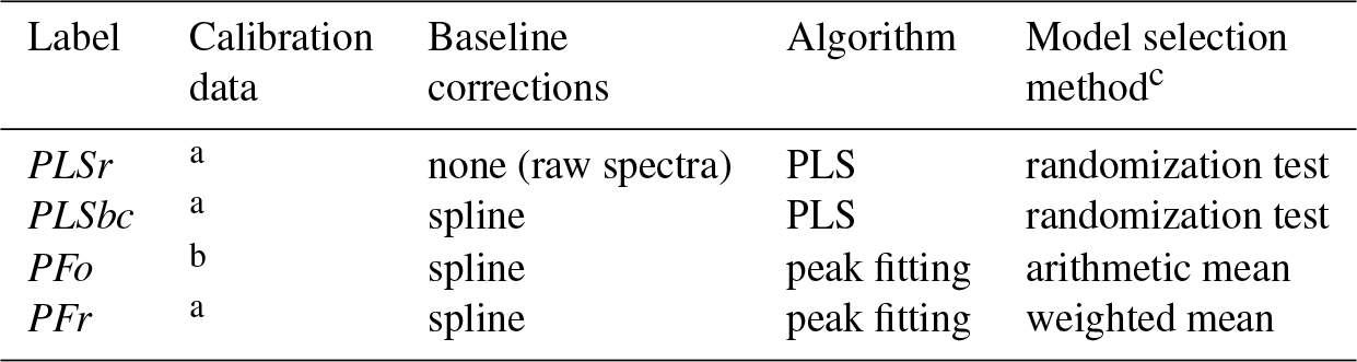
a Ruthenburg et al. (2014). b Gilardoni et al. (2007), Russell et al. (2010), and Takahama et al. (2013b). c For PLS, method for selecting number of LVs for each FG; for peak fitting, method for selecting an absorption coefficient for each FG.
2.1 Experimental data
We use 794 IMPROVE network PM2.5 samples and 238 laboratory standard samples reported by Ruthenburg et al. (2014), and we focus on the quantification of four organic functional groups and one additional inorganic group which absorbs in the same region: alcohol COH (aCOH), carboxylic COH (COOH), alkane CH (aCH), total (carboxylic, ketonic, and aldehydic) carbonyl (tCO), and inorganic ammonium NH (iNH). We report the evaluation of predictions for urban and rural sites separately. The urban sites consist of two collocated measurement stations in Phoenix, AZ, while the rural sites consist of five locations: Mesa Verde, CO; Olympic, WA; Proctor Maple Research Facility, VT; Sac and Fox, KS; St. Marks, FL; Trapper Creek, AK, spread throughout the United States.
Ambient samples were collected every third day from midnight to midnight (local time) for 24 h. FTIR spectra are obtained for PM collected on 25 mm PTFE filters (Teflon, Pall Gelman – 3.53 cm2 sample area) of the same type that are analyzed for gravimetric mass, elements and light absorption in the IMPROVE network. The nominal flow rate is 22.8 L min−1, which yields a volume of 32.8 m3 for 24 h. A Tensor 27 FT-IR spectrometer (Bruker Optics, Billerica, MA) equipped with a liquid-nitrogen-cooled wide-band mercury cadmium telluride detector is used to analyze the PTFE samples in transmission mode, using the empty sample compartment as the background. The sample compartment is continuously purged with air containing low levels of water vapor and CO2. Further details are provided by Ruthenburg et al. (2014) and Dillner and Takahama (2015a). TOR OC (and EC) mass is measured on quartz filters collected in parallel to the PTFE samples using the IMPROVE_A protocol (Chow et al., 2007). The TOR OC values are also adjusted for positive artifacts due to organic vapor adsorption onto quartz fiber by subtracting the monthly mean blank values. Sulfate and nitrate concentrations are measured on nylon filters also collected in parallel and analyzed by ion chromatography. Elemental composition is measured by X-ray fluorescence (XRF). The atmospheric concentrations of OC, nitrate, sulfate, and elemental composition provided by these techniques (obtained from the Federal Land Manager Environmental Database, FED, http://views.cira.colostate.edu/fed/Default.aspx, last access: 4 April 2019) are converted to equivalent areal mass densities on the PTFE filters using the filter collection area and actual sampled volume.
2.2 Spectral pretreatment
The baseline correction method of Kuzmiakova et al. (2016) is applied to both ambient and standard spectra for PF and PLS described below. This method uses smoothing splines (Reinsch, 1967) to model the baseline by regressing onto the background regions (where no analyte absorption is expected) as well as by interpolating through the analyte region. The calculated baseline is subtracted from the high-frequency region (>1500 cm−1) where stretching or bending modes of aCOH, aCH, cCOH, carbonyl CO, and amine NH are present (Shurvell, 2006). A single parameter effectively controls the curvature of the fitted baseline, and we select the value which minimizes the negative absorbance fraction (NAF). NAF represents the contribution of negative analyte absorbance to the total analyte absorbance :
where denotes the one-norm magnitude of a vector (summation of all absolute values of vector elements). NAF is calculated across the entire wavenumber range in the analyte part of in a given segment, excluding the CO2 absorbance band. Raw and baseline-corrected spectra are shown in Fig. 1.
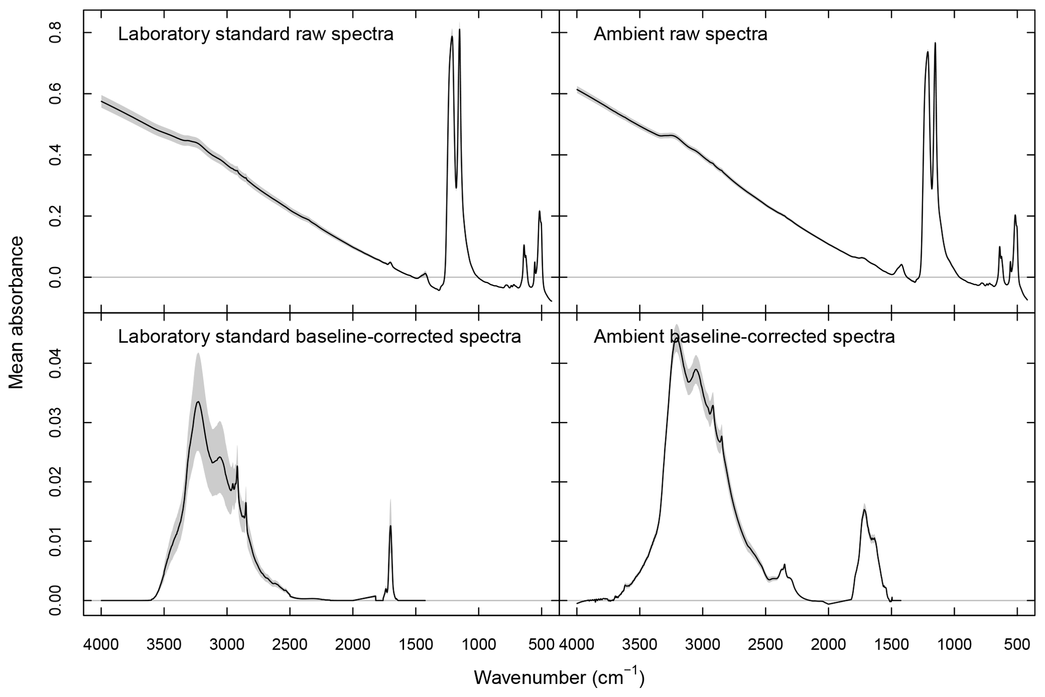
Figure 1Laboratory and ambient sample spectra (raw and baseline corrected). Black lines denote mean absorbances, and dashed gray areas denote 95 % confidence intervals.
2.3 Cluster analysis
Spectra similarities in baseline-corrected ambient sample spectra are used to group samples into clusters, as originally presented by Ruthenburg et al. (2014, appendix). We use Ward's hierarchical algorithm (Ward Jr., 1963), which has demonstrated useful categorizations in previous studies with FTIR spectra (e.g., Russell et al., 2009a; Takahama et al., 2011). Essentially, each baseline-corrected spectrum is normalized by its two-norm vector magnitude, and 20 clusters are selected to reduce the risk of grouping dissimilar samples together. Seven samples were excluded prior to cluster analysis and manually placed in three groups based on spectral similarity to known source profiles (Russell et al., 2011) (clusters 21 (n=2) and 22 (n=1)), or because the relative contribution of noise in low concentration samples would interfere with the clustering procedure (cluster 23 (n=4)). Clusters 19 (n=21) and 20 (n=19) were identified as being anomalous by Ruthenburg et al. (2014) when comparing FTIR-estimated OC to TOR OC. In this work, we identify two additional clusters which contain samples with anomalous predictions of organic FGs or iNH: clusters 7 (n=26) and 16 (n=12). Predictions and spectral characteristics for these four clusters are discussed separately, while the rest of the samples, classified as “rest” (n=706), are used for general evaluation.
2.4 Peak fitting
The method of PF constructs a physically based representation of absorbances based on Eq. (1), accounting for line shapes of spectral profiles resulting from absorption broadening. The fitted line shapes are constrained to be non-negative and within wavenumber limits derived from laboratory standards and ambient samples as described by Takahama et al. (2013b). To represent the essence of the PF algorithm in discretized notation, let s denote a line-shape function defined over wavenumbers , and an arbitrary set of peak parameters θ for sample i and bond k. The parameters are collectively estimated by nonlinear least squares fitting of overlapping curves to x to minimize the residual e over specific regions of interest. The areal density of bond n(a) is estimated as a product of the molar absorption coefficient and the integrated absorbance for each bond:
q denotes quadrature coefficients for numerical integration. for FTIR, so this term has been taken out of the summation. corresponds to the integrated absorption coefficient (which we report in units of ), which better characterizes the intensity of a dipole transition than ϵ when the absorption band spans a range of wavenumbers (Atkins and de Paula, 2006). We note that the use of these units marks a departure from previous convention of incorporating the filter collection area into the effective absorption coefficients (Maria et al., 2003; Gilardoni et al., 2007; Takahama et al., 2013b) ( cm2 in their work), but these units are preferred as they permit generalization across different filter sizes ( cm2 for Ruthenburg et al., 2014). For Gaussian line shapes used for both ambient and laboratory samples in this work, θik corresponds to any number of relevant amplitude, location, and width parameters for each bond, and an analytical solution exists for its integral. For fixed absorbance profiles (e.g., cCOH), the peak parameter corresponds to a scaling coefficient.
Typically, calibration parameters are obtained from single-compound standards where attribution of absorption to individual functional groups is the least ambiguous. Prediction in more complex mixtures is enabled by the concurrent fitting of multiple absorption peaks and invocation of mixing rules to arrive at a representative absorption coefficient. In this work, we retain the algorithm for apportioning the absorbance spectrum to various functional groups (Takahama et al., 2013b) and re-evaluate absorption coefficients using the calibration standards prepared by Ruthenburg et al. (2014). The apportionment protocol is based on initial values and constraints set out by analysis of a large number of laboratory and ambient samples as described by Takahama et al. (2013b). While peaks for FGs in laboratory standards only include those present in the compound, all FGs are assumed to be present in each sample, which is a convenient approximation in atmospheric samples. Regressing integrated absorbance against areal density, we fit linear models without intercept to each compound or mixture of compounds in accordance with the Beer–Lambert law (the value of the slope is unaffected by the inclusion of an intercept in this data set). We retain coefficients only for regressions which the coefficient of determination (R2) is greater than 0.9 and combine values from each compound or mixture i into a single coefficient (to be applied to ambient samples) for each FG k using the fractional number of samples as weights:
These weights are selected to generate comparable models to PLS, and for this reason we also include estimates of absorption coefficients in multicomponent mixtures in addition to single-component standards when the fitting quality criterion is met. The estimates using the original absorption coefficients (Russell et al., 2009a, 2010; Liu et al., 2009) will be referred to as PFo, and estimates using the recalibrated absorption coefficients will be referred to as PFr.
2.5 Multivariate calibration
Multivariate calibration is an alternative approach that is typically formulated as a linear regression problem, with the analyte concentration as the regressand (response variable) and absorbances used as regressors. In scalar notation, this relationship is written as
n(a) is the areal density for sample i and functional group k; x is the spectral absorbance, β is a wavenumber-specific regression coefficient, and e is the residual term. The number of wavenumbers at which absorbances are available exceeds the number of samples available for calibration (several thousand versus a few hundred), and the autocorrelation in absorbances due to the broadening leads to an underdetermined, collinear problem. Therefore, Eq. (4) must be solved by techniques other than classical least squares regression. PLS regression (Wold et al., 1984) is a generalization of multivariate multilinear regression and alleviates these problems by orthogonal projection and rank reduction (Geladi and Kowalski, 1986; Haaland and Thomas, 1988). Latent variables that maximize covariance with the response variable are found to model both the spectra matrix and response variables (FG abundances):
ℓ denotes the latent variable index, p and q are the loadings of x and na, respectively, and f and g are their residuals. The linear regression coefficients β in Eq. (4) are in turn derived from the loadings. In contrast to PF, multi-component reference standards that span the space of chemical composition are desired for PLS so that the ranges of composition – of both analytes and interferents – anticipated in prediction samples are available to train the model (Massart et al., 1988). As it is not possible to fully reproduce the high-dimensional chemical space of ambient samples, the amalgam of aerosol mixtures prepared in the laboratory targets the main features in this space.
A series of candidate models which satisfy Eqs. (4) and (5) is obtained by varying L, the maximum number of latent variables (LVs) or factors. The nonlinear iterative partial least squares (NIPALS) algorithm (Wold et al., 1983) is used to generate each model, and 10-fold Venetian blinds cross validation (Hastie et al., 2009; Arlot and Celisse, 2010) on the calibration set is applied to estimate corresponding root mean square of cross validation (RMSECV) values for the models. The minimum RMSECV solution is typically selected as the preferred model (defined by the value of L), but Takahama and Dillner (2015) found that this approach leads to overfitting with unrealistic results (i.e., extremely negative values) when extended to prediction of FGs in ambient samples. We therefore use the randomization test approach proposed by van der Voet (1994) to select the number of LVs. This method selects a model with fewer LVs for which the squared prediction error is not statistically greater than the reference (minimum RMSECV) model. This procedure is applied to each functional group separately such that each model is independent of one another (referred to as “PLS1” in chemometrics nomenclature). The number of LVs selected for PLSr and PLSbc are presented in Table S1 in the Supplement.
Though the interpretation of PLS models is less straightforward than PF, it is possible to examine how models are weighting spectral variables (wavenumbers) and calibration samples for making predictions. The regression coefficients are difficult to interpret directly as their magnitudes must be interpreted in combination with absorbances. In addition, the value of the regression coefficients can also be either positive or negative; the latter are associated with interfering species (Haaland and Thomas, 1988) or oscillations that increase with the number of LVs used (Gowen et al., 2011). Therefore, different approaches are used for estimating the contribution of specific wavenumbers to predictions. Takahama et al. (2016) used sparse calibration approaches that eliminated uninformative wavenumbers and used importance weighting to identify absorption bands used by PLS models. Wavenumbers highlighted by FG calibration models were associated with absorption bands of the target FGs while retaining similar prediction capability to the full wavenumber models presented here. The contribution of LVs to the explained variation and sum of squares of the spectra matrix and response variable are discussed in Sect. S4. The relationship between Eqs. (4) and (1) is illustrated in Sect. S1.
2.6 OC estimation from FG abundance
The constituent molar abundance na for atom a is calculated from the moles nk of FG k through a coefficient λak such that na=λaknk. From na estimated for {C, O, H} in this work, the OC mass, OM∕OC mass ratio, and O∕C atomic ratios are obtained. While assignment of λak for non-carbon atoms is unambiguous, λC⋅k depends on the assumed bonding configuration of polyfunctional carbon atoms (Takahama and Ruggeri, 2017). For instance, methylene (-CH2-) carbon has a value of (1 mol of carbon for two aCH groups), while methyl carbon (-CH3) has a value of . It is also possible for the same carbon atoms to be associated with both aCH and aCOH, or other FGs, which makes the selection of λ less intuitive with increasing number of combinations; several statistical approaches are available for estimation in these instances. The only difference between Russell and coworkers (Russell, 2003; Takahama et al., 2013b) and Ruthenburg et al. (2014) is the value of λC⋅aCOH; the former authors define the value as 0.5 and the latter authors define it as 0. Overall, the choice of this value makes a ∼10 % difference in the carbon estimate for this data set. For this work we adopt the value of 0.5, which is also supported by a recent analysis of modeled α-pinene secondary organic aerosol (Ruggeri and Takahama, 2016; Takahama and Ruggeri, 2017) according to the Master Chemical Mechanism (Jenkin et al., 1997; Saunders et al., 2003). The full set of coefficients is provided in Sect. S1. We refer to the OC reconstructed through FG predictions as FG OC in this paper.
2.7 Quantification of carboxylic acid and non-acid carbonyl groups
While the carboxylic group comprises two molecular bonds, the abundances of carboxylic hydroxyl and carbonyl bonds are conventionally quantified separately with calibration models developed for their respective absorption bands. The carbonyl quantified in this way can include contributions from ketonic and aldehydic carbonyl because of their proximity in absorption bands that are difficult to resolve in environmental samples; the carboxylic hydroxyl cCOH and total carbonyl tCO are re-apportioned to estimate abundance of carboxylic COOH groups along with non-acid (ketonic, aldehyde, and ester) carbonyl CO (written as naCO). Stoichiometrically, nCOOH and ncCOH are equivalent, while nnaCO is simply the difference between ntCO and ncCOH (Eq. S1 in the Supplement). In principle, the exact molar composition in a mixture should meet the condition that the tCO is in excess of the cCOH (ntCO≥ncCOH), with naCO content indicated by the tCO in excess of cCOH. To account for random errors, Takahama et al. (2013b) recommend the averaging of cCOH and tCO to estimate COOH when ntCO∼ncCOH. The estimated cCOH can be greater than tCO ncCOH<ntCO if the integrated absorption area or absorption coefficient is misspecified for either FG. In the absence of additional information, Takahama et al. (2013b) assume that the tCO is unmeasured due to shift in absorption frequency below that used in PF, and they base the COOH estimate on the cCOH. In such cases, an overall unmeasured fraction was assigned on a per-campaign basis to align tCO to cCOH abundances in previous studies, but in this work we apply this reasoning on a per-sample basis (i.e., nCOOH≡ncCOH and ).
One strategy to avoid the apportionment of tCO to COOH and naCO is to build an alternative PLS regression model to predict naCO directly, rather than tCO. The known concentrations in laboratory standards are transformed according to Eq. (S1) and provided as the response vectors to Eq. (4). In this work, the contributions to naCO in calibration standards are provided by 12-tricosanone and arachidyl dodecanoate, and therefore correspond to ketone and ester CO (i.e., no aldehyde CO). Previous studies atomizing dissolved aldehydic compounds found that they were transformed into alcohols by aldol condensation, which is also a possible but not a necessary outcome in the atmosphere (Takahama et al., 2013b) and depends on the presence of water and hydration constant of the compound. Nonetheless, we will refer to our new estimates as naCO under the assumption that aldehyde CO, if present in ambient samples, has a similar spectroscopic response to ketone and ester CO to the extent that we can quantify them. The COOH calibration remains identical to that for cCOH since nCOOH≡ncCOH, and the stoichiometric consistencies for estimating OC, OM, OM∕OC, and O∕C ratios using different estimates of carbonyl are summarized in Sect. S1.
2.8 Evaluation metrics
Metrics such as mean error, mean bias, RMSE, and many others exist for intercomparison among measured and estimated values. In this work, to quantify overall bias we use total least squares slope (obtained via major axis regression), which accounts for uncertainties in both quantities being compared (Ripley and Thompson, 1987), and the Pearson's correlation coefficient (r) to quantify the strength of linear relationship between the two quantities. Values estimated with slopes and r close to unity among different methods are considered more robust. All evaluation metrics provided are for samples labeled as cluster “rest”, excluding clusters 7, 16, 19, and 20.
We first report on differences among estimated absorption coefficients (Sect. 3.1). In Sect. 3.2 and 3.3, we evaluate and discuss the FG estimated using the PF (using original and recalibrated absorption coefficients) and PLS (using baseline-corrected and raw spectra) methods.
3.1 Estimation of absorption coefficients
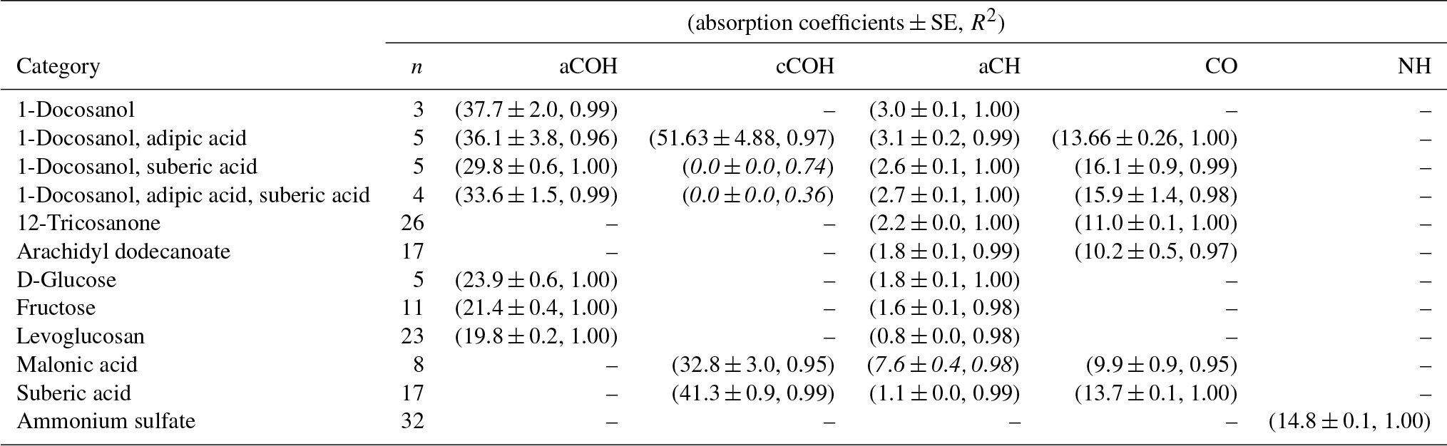
Calibration curves and predicted concentrations according to the PF strategy outlined in Sect. 2 are shown in Fig. 2. The top row refers to the calibration curves to compute the absorption coefficients (obtained using two-thirds of the 238 laboratory standards), and the bottom row refers to the evaluation of derived absorption coefficients on predicted concentrations for test set compounds not used in the calibration. Regression parameters including the number of samples used in each category, n, are included in Table 2. Absorption coefficients are estimated for cCOH by two mixtures (italic values in Table 2): (1) 1-docosanol and suberic acid, and (2) 1-docosanol, suberic acid, and adipic acid are not included in the calibration because of their low R2 values. Malonic acid samples are additionally excluded in the estimation of aCH as its concentration range is far below the rest of the laboratory standards (below typical loadings of atmospheric samples) and the slope is twice greater than the next highest value (italic values in Table 2). This difference biases the weighted absorption coefficient in a way that does not reflect the weighting of the PLS regression (including this value makes a 19.9 % difference in the absorption coefficient). Overall, we used 97 % of the laboratory standard samples, of which two-thirds were reserved for the calibration (Figs. S1–S4 in Sect. S5). We can see that when the absorption coefficient for each respective category is applied to corresponding test set samples not used in the calibration (the remaining one-third of samples), predictions are within 6 % of the reference values (Fig. 2, bottom row).
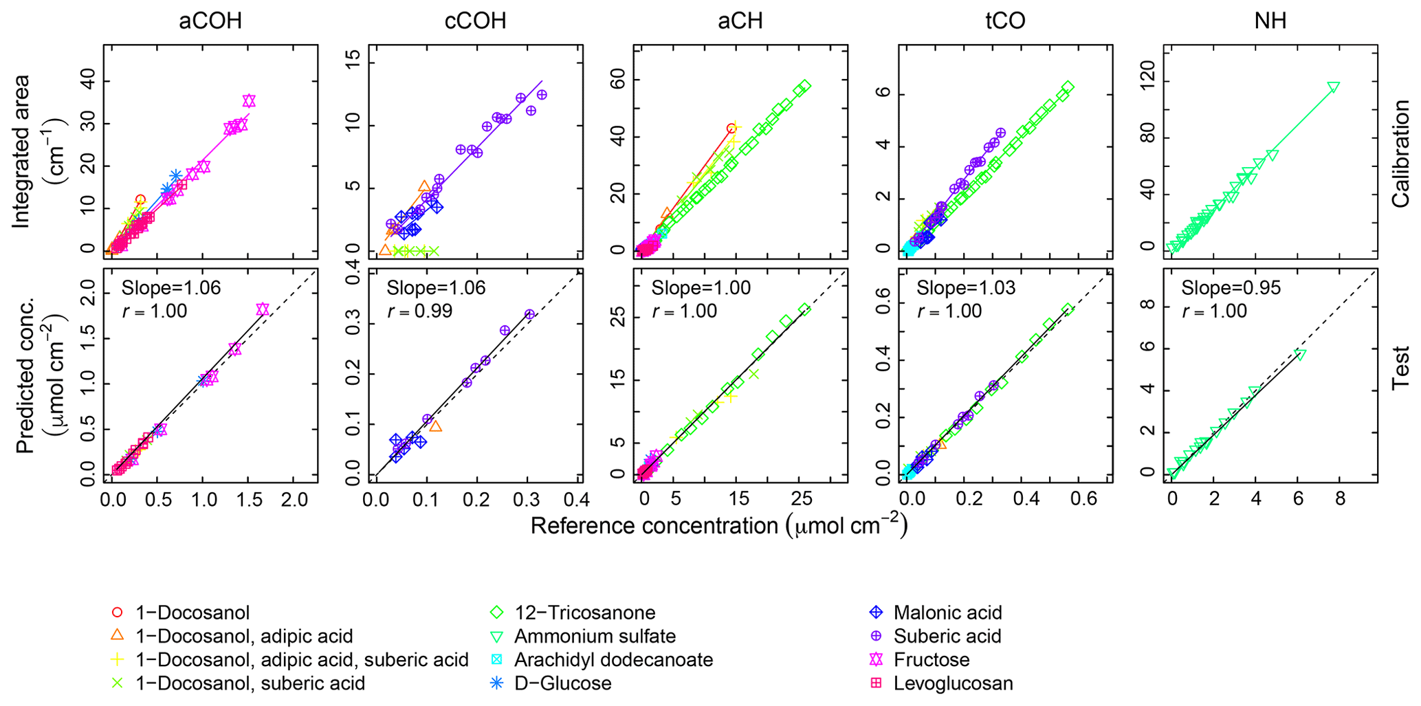
Figure 2Top row: integrated absorption as a function of known molar abundance used to derive molar absorption coefficients. Bottom row: evaluation of derived absorption coefficients on predicted concentrations for test set compounds not used in the fitting.
Table 2Recalibrated absorption coefficients and fit statistics for each FG and compound. Italicized texts denote the compounds not used in the computation of cCOH and aCH absorption coefficients averages.
In Fig. 3, we compare the new absorption coefficients with those summarized by Takahama et al. (2013b) (specific citations described in figure caption) adjusted for filter collection area. aCOH for 1-docosanol is the only FG and organic compound for which we have a direct comparison; the value estimated for the absorption coefficient in this work is 3.6 times greater. This is due to different baseline correction methods and fitting procedures used by Gilardoni et al. (2007). When the same spectra preparation (smoothing spline baseline correction) is applied, the difference is 2 times greater but occurs in the same proportion for aCH absorption – i.e., both aCOH and aCH absorption coefficients for 1-docosanol spectra (n=3) acquired by Ruthenburg et al. (2014) are twice that for spectra acquired by Gilardoni et al. (2007) (n=6) when processed in the same way, but the ratio of aCOH to aCH absorbances for each method is within 4 %. This bias may partially be due to the fact that the slope of the calibration curve is determined by a single influential point for the few pure 1-docosanol samples collected by Ruthenburg et al. (2014). However, the consistency of the single-point estimate with aCOH coefficients for other mixtures containing 1-docosanol (Fig. 3) may suggest other differences that need to be investigated. For instance, the refractive index of the substrate may also affect the apparent absorbance in the limit of thin films (Hasegawa, 2017); similarity in optical properties of the filter type may have to be considered in future studies. Single measurements of fructose, glucose, as well as nine other sugars, were combined to derive an overall absorption coefficient for saccharides by Takahama et al. (2013b) (point estimates for fructose are effectively the same as the combined estimate, and glucose is 70 % smaller; Russell et al., 2010, Table S2). We observe that the absorption coefficients for individual compounds in this work are higher than the previous collective estimate. While there was previously no calibration performed for ammonium sulfate for its quantification by PF, the single ammonium sulfate sample used for removal of ammonium interference in the fitting procedure (introduced by Russell et al., 2009a) carried a mass of 6.0 µg over a cm2 collection area (Takahama et al., 2013b), so this value is used to calculate a point estimate for its absorption coefficient. The recalibrated absorption coefficient is greater by a factor of 1.7. This is likely due to the combination of using a single-point value for estimating the coefficient.
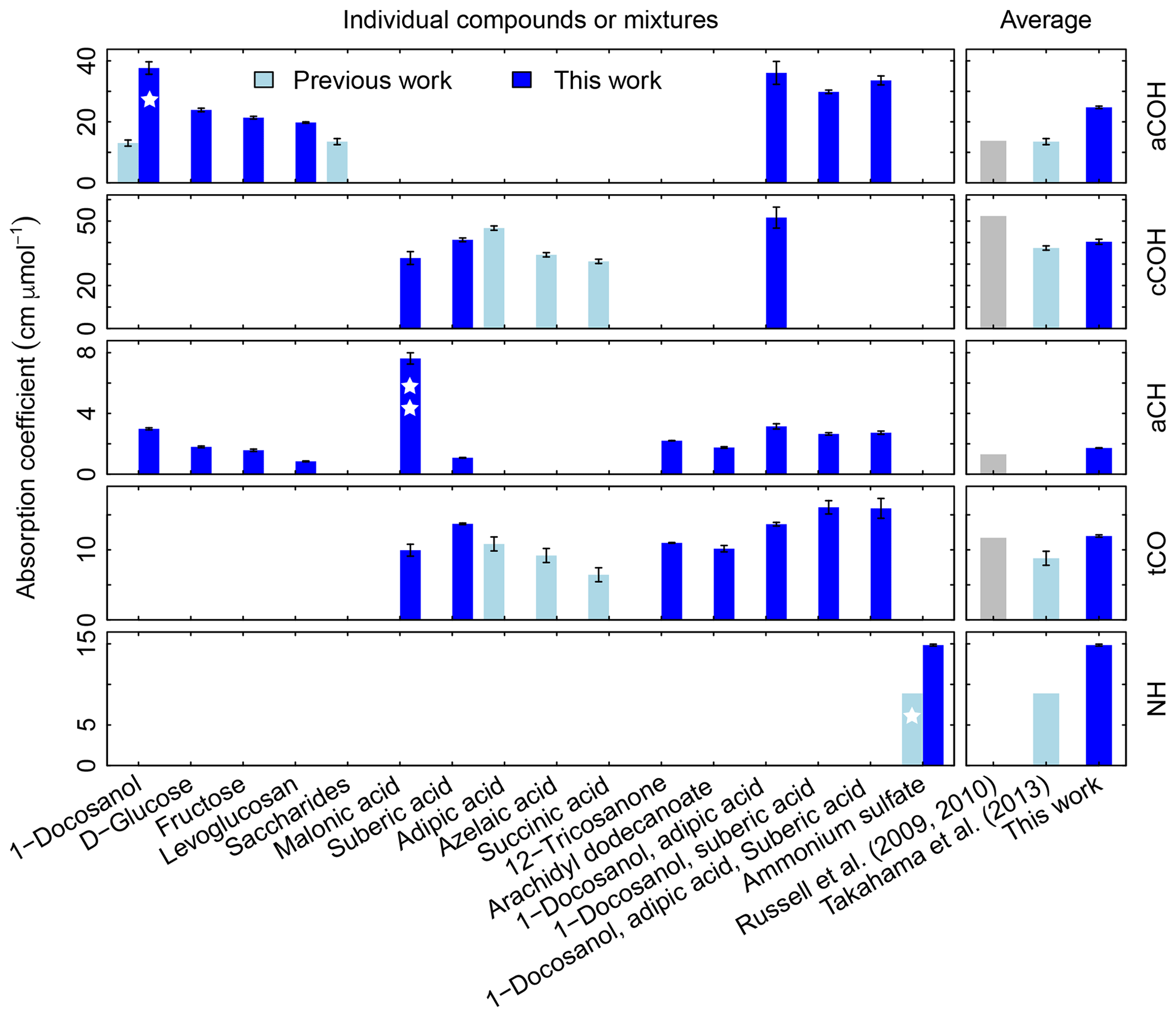
Figure 3Summary of molar absorption coefficients reported in the literature. The single star for 1-docosanol aCOH indicates that there are only three points – one of which is an influential point – so this is effectively a single-point estimate. The single star for ammonium sulfate indicates that it based on a single value. The double star is used to indicate that the absorption coefficient for malonic acid cCOH is estimated for a concentration range order of magnitude lower than the rest. Previous studies are summarized by Takahama et al. (2013b), which also compiled coefficients from Gilardoni et al. (2007) and Russell et al. (2010). The error bars represent plus/minus one standard error of the molar absorption coefficients.
Absorption coefficients for aCH vary by a factor of 3.2 (between 1.0 and 3.2, over 10 compounds), for aCOH by a factor of 1.9 (between 19.8 and 37.7, over seven compounds), for cCOH by a factor of 1.6 (between 32.8 and 51.6, over three compounds), and for tCO by a factor 1.6 (between 10.0 and 16.1, over seven standards; Fig. S11). Without informed strategies for parameter selection, the range of valid possibilities for these absorption coefficients imparts uncertainty in FG calibration.
Shown on the right side of the Fig. 3 are averaged values reported by Russell and coworkers (Gilardoni et al., 2007; Russell et al., 2009a, 2010; Takahama et al., 2013b) and this work. Both sets will be compared in the following sections. The FG absorption coefficients for aCOH and aCH estimated in this work are higher by a factor of 1.8 and 1.3 respectively, which leads to lower estimates for FG abundances. In contrast, the FG absorption coefficient for cCOH is lower than that reported by Russell et al. (2009a) (factor of 0.8) and comparable to the one reported by Takahama et al. (2013b). The FG absorption coefficient for tCO is comparable with the one of Russell et al. (2009a) and 1.4 times greater than the one reported by Takahama et al. (2013b).
3.2 Comparison of estimated OC and ammonium to external measurements
We first compare quantities for which we have an independent estimate (TOR OC and ammonium) to place our predictions in context. Individual contributions of FGs used to estimate OC are discussed in Sect. 3.3. Comparisons are stated for regular samples not belonging to anomalous clusters (Sect. 2) unless otherwise noted. Evaluation of anomalous clusters is discussed separately in Sect. 3.6.

Figure 4Comparison of estimated OC (FG OC) against OC measured by TOR method (TOR OC). PFo refers to peak fitting using the original parameters. PLSr refers to partial least square using raw spectra. PFr refers to peak fitting using the recalibrated absorption coefficients. PLSbc refers to partial least square using baseline-corrected spectra.
Figure 4 summarizes the comparison of predicted concentrations of OC using different sets of absorption coefficients (for PF – PFo and PFr refer to PF using the original and the recalibrated absorbance coefficients respectively) or different spectra pretreatment (for PLS – PLSbc and PLSr refer to PLS using the baseline-corrected and unprocessed spectra respectively). In general, the correlation between TOR OC and FG OC is high (r= 0.84–0.97) and typically greater for urban sites than for rural ones. In the urban samples, OC estimated by PLSr is closer to TOR OC with an underprediction of 12 %, while the other methods underpredict TOR OC by 34 %–50 %. In the rural sites, the agreement with TOR OC is more varied with three models underpredicting TOR OC by 0 %–22 % and PLSbc by 40 %. In general, the consistent underprediction is expected on account of the undetectable carbon atoms by FTIR due to lack of functionalization or association solely with bonds we do not measure.
The difference between PFo and PFr is due to the systematic increase in absorption coefficients used by PFr compared with PFo, which decreases the molar abundance of FGs and, consequently, the FG OC. This difference is particularly articulated by the absorption coefficient for aCH (1.73 against 1.31) as its mole fraction is over 60 % regardless of estimation method used.
The differences between PLSr and PLSbc are more difficult to understand, but some interpretations can be made. First, systematic differences can occur in the way that laboratory standard and ambient sample spectra are baseline corrected as the absorbance regions are different. Also, baseline correction used in the PLSbc does not include frequency lower than 1500 cm−1, thus excluding the alkane peak around 1450 cm−1 that is likely being used for aCH estimation by the PLSr model (Takahama et al., 2016). As FG abundances in laboratory samples are reproduced with minimal error, we anticipate that PTFE interferences to predictions are minimal with PLSr. However, PLSr may be erroneously incorporating some information regarding the scattering by supermicron particles in its prediction (Sect. 3.6). Notably, the samples labeled as anomalous by Ruthenburg et al. (2014) (clusters 19 and 20) are predicted more consistently in relation to TOR OC with PLSbc than PLSr, suggesting the baseline correction has partially removed spectral features from the raw spectra that lead to unexpected deviations in predictions. For the remaining samples, it is generally possible to find models – using raw or baseline-corrected spectra – with different parameters (e.g., a different number of LVs) that produce similar predictions and also models in which FG OC agrees better with TOR OC. While we do not explore all possible combinations of parameters exhaustively in this paper, an example of how comparisons of FG OC predictions vary with number of LVs of aCH for PLS with baseline corrected is given in Fig. S16. The solution that best matches TOR OC (referred to as PLSbc*) from this evaluation is shown in Fig. 5.
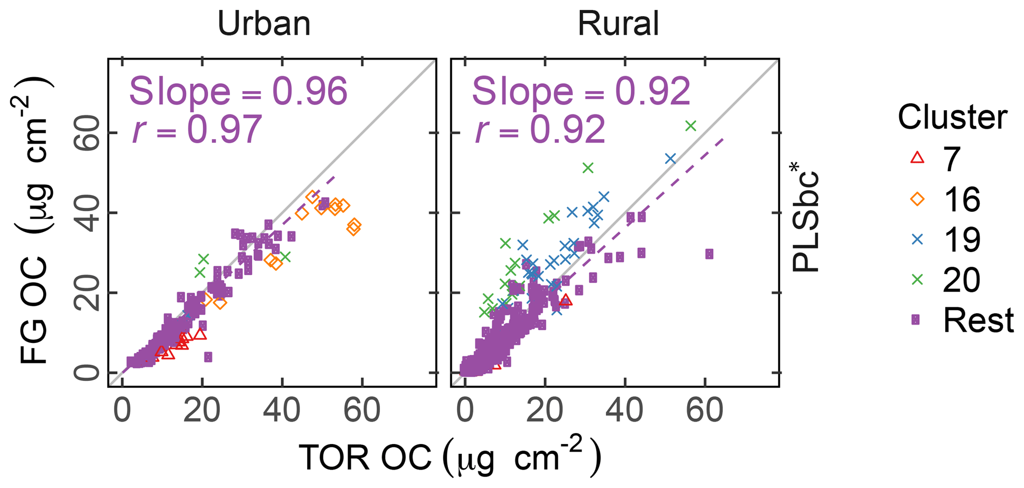
Figure 5Comparison of estimated OC (FG OC) gainst OC measured by TOR method (TOR OC). PLSbc* refers to partial least square using baseline-corrected spectra and a heuristic choice for the aCH LVs number (13) based on agreement between FG OC and TOR OC (Fig. S16).
The solutions in the neighborhood (±3 LVs) of the PLSbc models for each FG are highly correlated, but they vary in their slope by a factor of approximately 1.5 (Sect. S8). PLSbc* varies from PLSbc for aCH by only 2 LVs.
PLSbc* is only one of many possible models that show improved agreement with TOR OC to be explored in future work; for this paper we restrict our evaluation of results primarily to those obtained by the protocols described in Sect. 2.
Figure 6 summarizes the comparison of ammonium concentrations predicted by FTIR with the value estimated as the cation counterpart of sulfate and nitrate. The correlation in comparisons is strong for rural sites (r>0.89) and moderately strong (r= 0.47–0.71) in urban sites for all models. Part of this difference may be that the dynamic range of ammonium in rural sites is twice the value of urban sites. While our estimated reference values are thought to be the upper bound of ammonium concentrations (on account of our assumptions that (i) there is neither evaporation loss of ammonium nitrate from PTFE nor (ii) nitrate association with dust instead of ammonium), the reference ammonium is overpredicted by the PSLr model at urban sites and by the PFo model at both urban and rural sites. The PFo overpredictions can be explained by the uncertainty on the absorption coefficient estimated using a single value. The overprediction in urban sites only by PLSr is less simple to interpret. One possibility is the scattering contribution to the FTIR spectra by large particles may be more significant for these samples, and this effect is reduced by baseline correction.
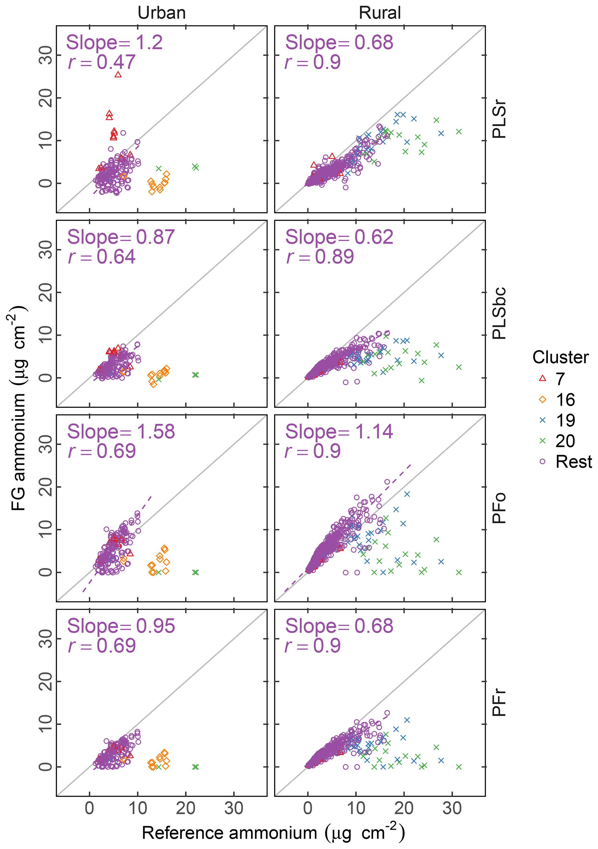
Figure 6Comparison of estimated ammonium (FG ammonium) against ammonium measured using ion chromatography (IC ammonium). PFo refers to peak fitting using the original parameters. PLSr refers to partial least square using raw spectra. PFr refers to peak fitting using the recalibrated absorption coefficients. PLSbc refers to partial least square using baseline-corrected spectra.
While ammonium quantification by FTIR has been the focus of past researchers (Johnson et al., 1981; McClenny et al., 1985; Allen et al., 1994; Krost and McClenny, 1994; Reff et al., 2007), the recent work of Russell, Dillner, and co-workers focused on organic FG quantification, and an extensive evaluation for ammonium has not been performed. However, as the absorption bands of iNH overlap with aCOH, cCOH, and aCH, it is useful to know whether the fitted ammonium scales with an external measurement. Such a simultaneous evaluation of bonds is important for PF, since the IR absorption in each spectrum is apportioned to contributions from various bonds; overapportionment for one bond can lead to underapportionment for another. Based on the assessment with PFr using a better-characterized absorption coefficient, comparisons with the reference ammonium values suggest that neither gross overestimation nor underestimation of the fitting is likely. Calibration models for PLSr and PLSbc used in this work are developed independently of one another (the “PLS1” approach); therefore, the predictive capability of one species is not strongly tied to another as with PF. In summary, the LVs in the ammonium calibration model are not necessarily the same as the organic FGs; the over- or underprediction of ammonium is less consequential to how we interpret the FG quantifications. An alternative, multimodel formulation (“PLS2”) can provide estimates of both analyte and interferents using the same set of LVs. The current decision to use PLS1 is based on the knowledge that PLS1 typically outperforms PLS2 as it is optimized for each target analyte (Martens and Næs, 1991), but in extrapolation (as in our use case) the physically consistency offered by PLS2 may confer benefits not conventionally recognized with such models.
3.3 Variations in estimated FGs
Figure 7 summarizes pairwise correlation coefficients and regression slopes (excluding anomalous clusters 7, 16, 19, and 20) of FG abundances estimated using the methods discussed in Sect. 3.2. Individual scatter plots can be found in the Supplement (Figs. S5–S9). Overall, aCH, iNH, and tCO, agree with fairly high correlation r>0.75, but the agreement of aCOH and cCOH – two FGs with broad absorption regions on account of the OH stretch – varies more significantly. The strong agreement of iNH predicted by PLS and PF is particularly notable. While the calibration models for PLSr and PLSbc are formulated to predict ammonium iNH, they are technically equivalent to a calibration model for ammonium sulfate as this is the only substance with this bond in the calibration set. However, the comparison of predictions against PF, which only uses the NH stretching peak – which are spectroscopically similar between ammonium nitrate and sulfate – suggests that the PLS models are likely using features that are specific to this absorption band that is common to both ammonium salts.
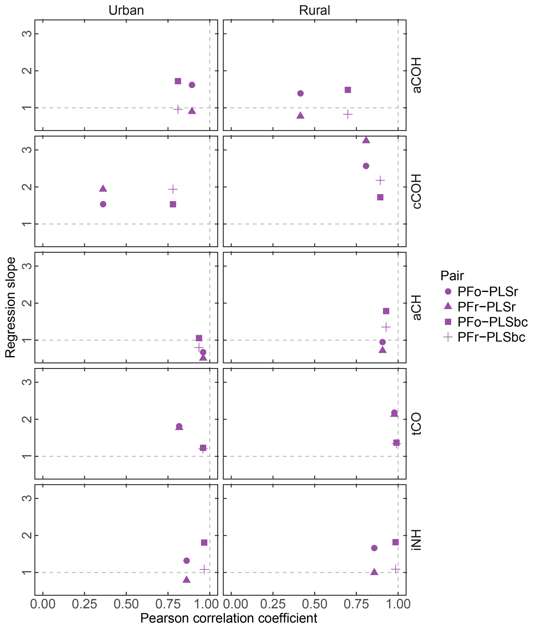
Figure 7FG comparison summary. Pearson correlation coefficient PFo refers to peak fitting using the original parameters. PLSr refers to partial least square using raw spectra. PFr refers to peak fitting using the recalibrated absorption coefficients. PLSbc refers to partial least square using baseline-corrected spectra.
First, we focus on the comparison between PFo and PLSr. In urban samples, aCH presents the highest correlation (r=0.96) of all FGs, presumably, because the aCH absorption is unambiguous on account of the high abundance of hydrocarbon compounds in urban areas. However, the slope (0.68) reveals a systematic difference between the two. For the rest of the organic FGs in both urban and rural sites, PFo estimates are higher than PLSr; the regression slopes vary between 1.39 (aCOH in rural samples) and 2.57 (cCOH in rural samples).
Correlation coefficients in the PFr–PLSr comparison for any organic FG are similar to the PFo–PLSr comparison; the only notable difference is the larger regression slope for cCOH (1.94 and 3.25 for urban and rural samples against 1.53 and 2.57 respectively), due to the lower absorption coefficient applied to PFr than PFo (Table 2). The cCOH and tCO estimated by PFr are still higher than PLSr (by 1.78 to 3.25). However, the underprediction of FG OC relative to TOR OC (Sect. 3.2) can be explained by the lower concentrations of aCH and aCOH estimated with the recalibrated absorption coefficients as they compose more than 70 % of the organic aerosol mass according to PF analysis (Sect. 3.5).
PFo and PFr predictions agree closely with PLSbc, likely because they use the same portion of the spectra. The organic FG correlations vary between 0.7 (aCOH – rural samples) and 0.99 (tCO – rural sample). PFr predictions are closer to PLSbc than PFo, with the exception of cCOH, since they use the same laboratory standard compounds.
The correlation for iNH is greater than 0.97 with slope close to one in the case of PFr and greater than 1.8 in the case of PFo, which indicates a systematic bias due to the different absorption coefficients used (14.84 and 8.89 for PFr and PFo respectively).
The correlations in tCO between PF and PLS are high (r>0.81), potentially because of the narrow absorption band of the carbonyl FG. PF estimates of tCO for urban samples increase in correlation with PLS estimates from 0.82 to 0.96 (with the slope approaching unity) when baseline-corrected spectra are used for PLS, suggesting that signal contributions (presumably from PTFE) interfering from the quantification are effectively removed.
Within the broader scope of assessing uncertainty for each FG, we can consider that the estimated slopes can vary according to the selection of absorption coefficient value for PF and the number of LVs for PLS. The range of absorption coefficients is given in Sect. 3.1, with aCH having the largest range. If we examine the set of PLSbc solutions (varying only in number of LVs) with a correlation coefficient greater than 0.95 with the selected solutions presented here, we find that the largest variability is also in the aCH (ranges are shown in Fig. S11 and differences among models in Fig. S12). Models with different number of LVs reflect different weighting of calibration samples and their responses, so it is not surprising to find that the magnitude of uncertainties (reported in Sect. 3.1) is similar between PLS and PF for the same set of calibration standards.
3.4 Quantification of carboxylic acid and non-acid carbonyl
Figure 8 compares the abundance of tCO and cCOH predicted by the four methods. Both PLSr and PLSbc predict similar abundances of tCO as cCOH, suggesting that most of the carbonyl is associated with carboxylic acid groups, and the non-acid fraction is small to negligible. While it is possible for both models to use the carbonyl absorption band, Takahama et al. (2016) suggest that the wavenumbers are weighted differently by the two models.
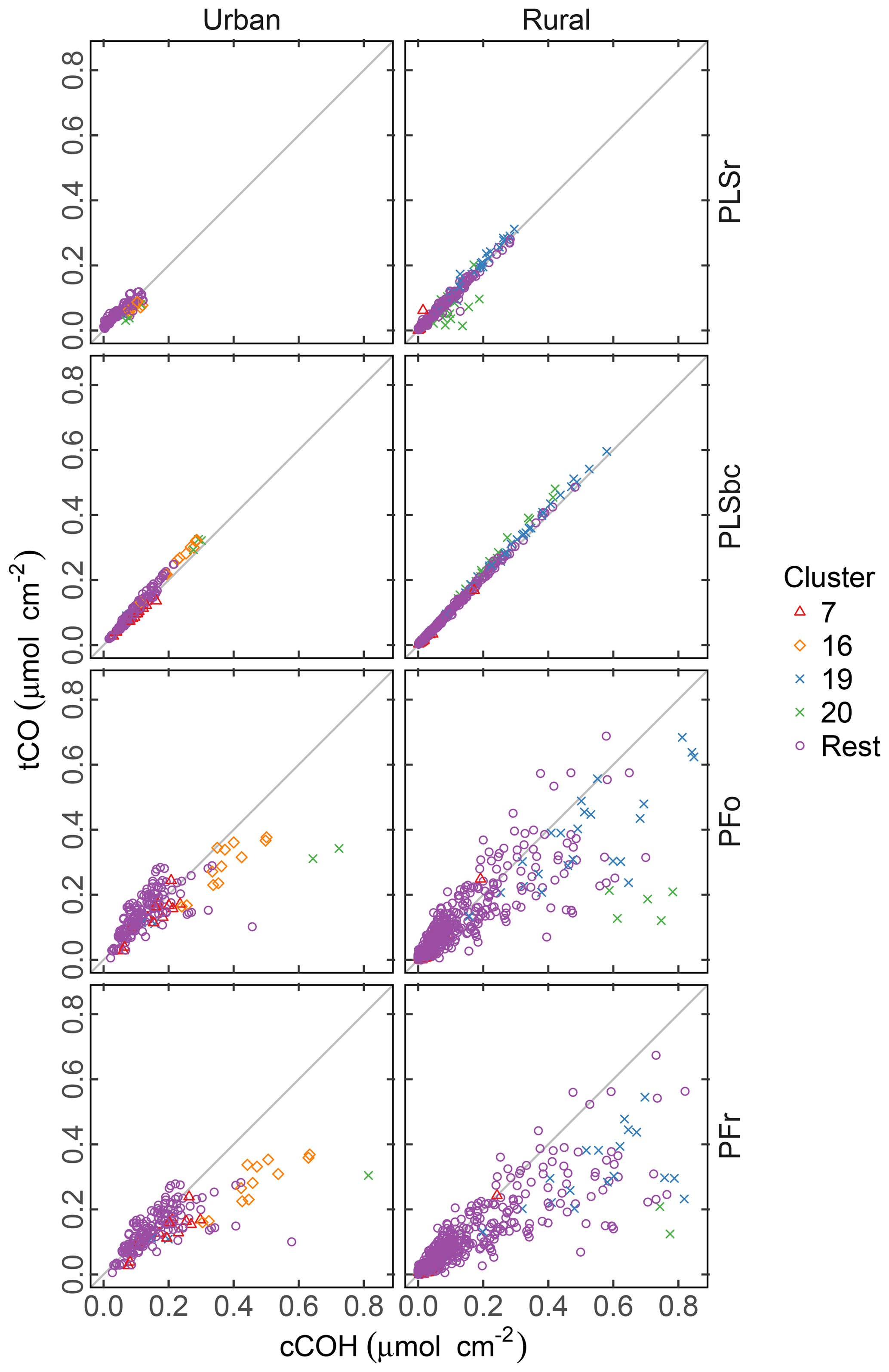
Figure 8Comparison of quantified abundance of tCO and cCOH. PFo refers to peak fitting using the original parameters. PLSr refers to partial least square using raw spectra. PFr refers to peak fitting using the recalibrated absorption coefficients. PLSbc refers to partial least square using baseline-corrected spectra.
There is noticeably more scatter in the relationship between tCO and cCOH from the PF predictions, with the presence of naCO difficult to identify in these samples. Furthermore, tCO abundance is systematically lower than cCOH for many samples (discernable beyond the extent of scatter). Takahama et al. (2013b) hypothesized that this discrepancy could be due to underestimation of carbonyl in samples where the absorption band is shifted to lower frequencies. However, given that (1) the constraint ntCO≥ncCOH is met for the PLS estimates, and (2) the relative overprediction by PF in comparison to PLS is greater for cCOH than tCO in these samples, it is likely that it is cCOH that is overestimated by PF for these samples. This may be due to the peak profile for cCOH or baseline correction artifacts. For clusters 19 and 20 in which the overestimation is more severe, the baseline correction artifact is the most probable reason as discussed in Sect. 3.6.
Figure 9 compares the estimated naCO for two methods of calibration: one estimated through the difference of tCO and COOH (the canonical approach) and by direct calibration (alternate approach). We find that, on average, the naCO is close to zero using both estimates (and within the differences of cCOH and tCO). For predictions with raw spectra, the range of predictions is smaller for naCO estimated directly than as a difference of cCOH and tCO. naCO estimates from PLS with baseline-corrected spectra are notably less variable than for those using raw spectra. Moreover, the canonical and alternate estimates are strongly correlated (r=0.99 for urban and r=0.95 for rural samples) even for these low concentrations, despite the fact that the two models use wavenumbers and latent variables differently (Fig. S13). These results suggest that baseline correction can reduce interferences that may impart uncertainties in the estimation of FGs in this region for most samples, including clusters 7, 16, and 20.
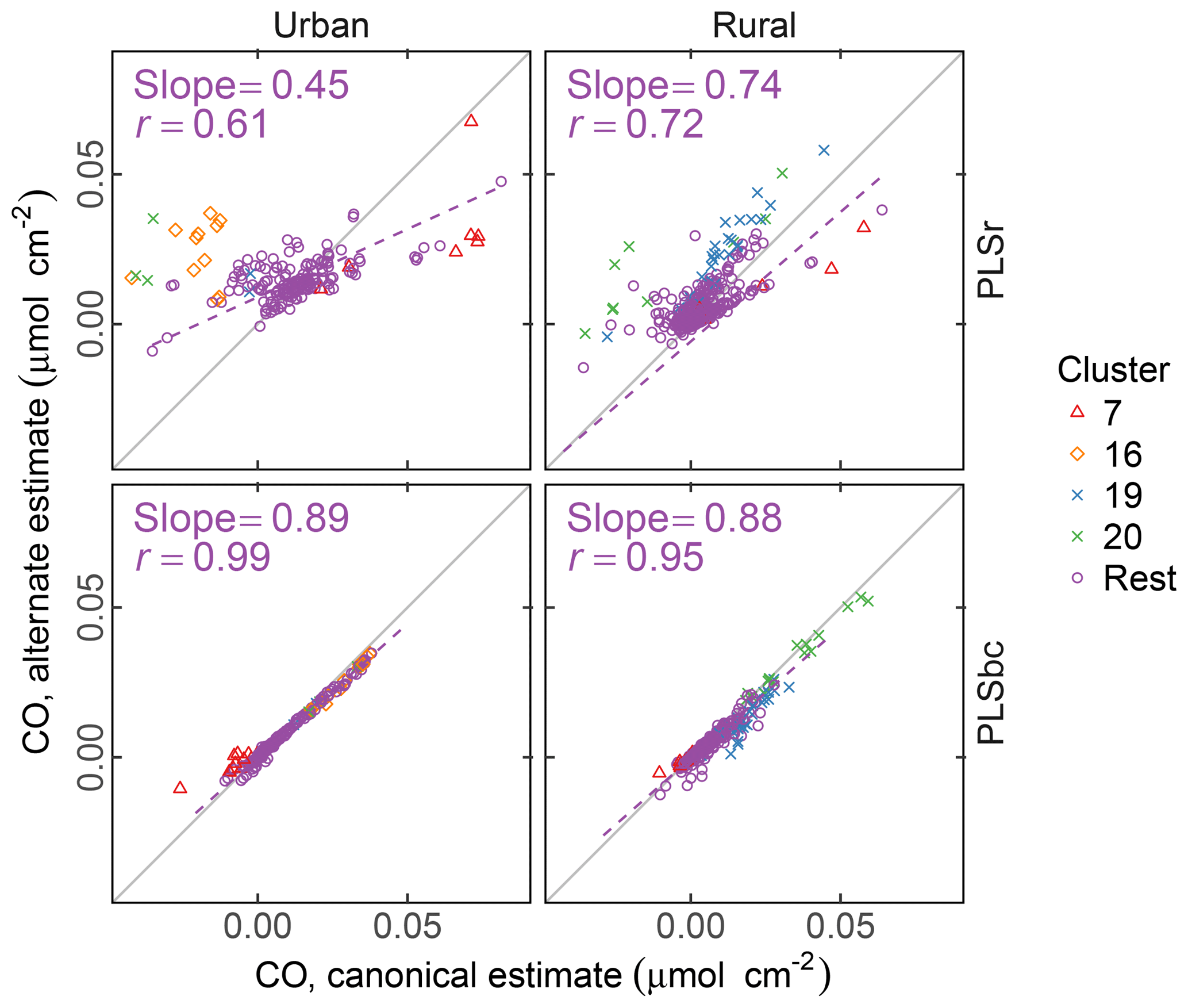
Figure 9Comparison of estimated CO according to canonical calibration (as difference between molar abundance of cCOH and tCO), and alternate calibration (direct calibration to non-acid CO). PLSr refers to partial least square using raw spectra. PLSbc refers to partial least square using baseline-corrected spectra.
High abundances of naCO have been reported in biomass burning and biogenic secondary OM in past studies (using PF), either due to ketones present in photochemical reaction products (Schwartz et al., 2010) or esterification in the condensed phase (Russell et al., 2011). Therefore, it is surprising to find such low abundances of naCO especially in rural sites with biogenic influences and samples influenced by residential wood burning (Kuzmiakova, 2019). This finding may point to a differences in sample types between this and previous work, as well as possible artifacts due to long PM collection times, storage, and transport protocols in monitoring network samples. For instance, more opportunities for conversion of naCO to aCOH by aldol condensation in the condensed phase may be possible in these samples.
3.5 Evaluation of estimated OM, OM∕OC, and O∕C
Figure 10 (left column) summarizes estimates of OM, OM∕OC, and O∕C obtained by FTIR (distributions are shown in Fig. S14). On average, concentrations of OM are higher in urban samples than rural ones, while the OM∕OC ratio and O∕C ratio shows the opposite pattern, as expected from previous studies. These trends are in agreement with measurements by GC-MS and AMS (Turpin and Lim, 2001; Aiken et al., 2008), and they are in accordance with our understanding of atmospheric processes by which condensation of functionalized molecules (Ziemann, 2005; Kroll and Seinfeld, 2008) and heterogeneous reactions (Smith et al., 2009; Lim et al., 2010) lead to chemical aging.
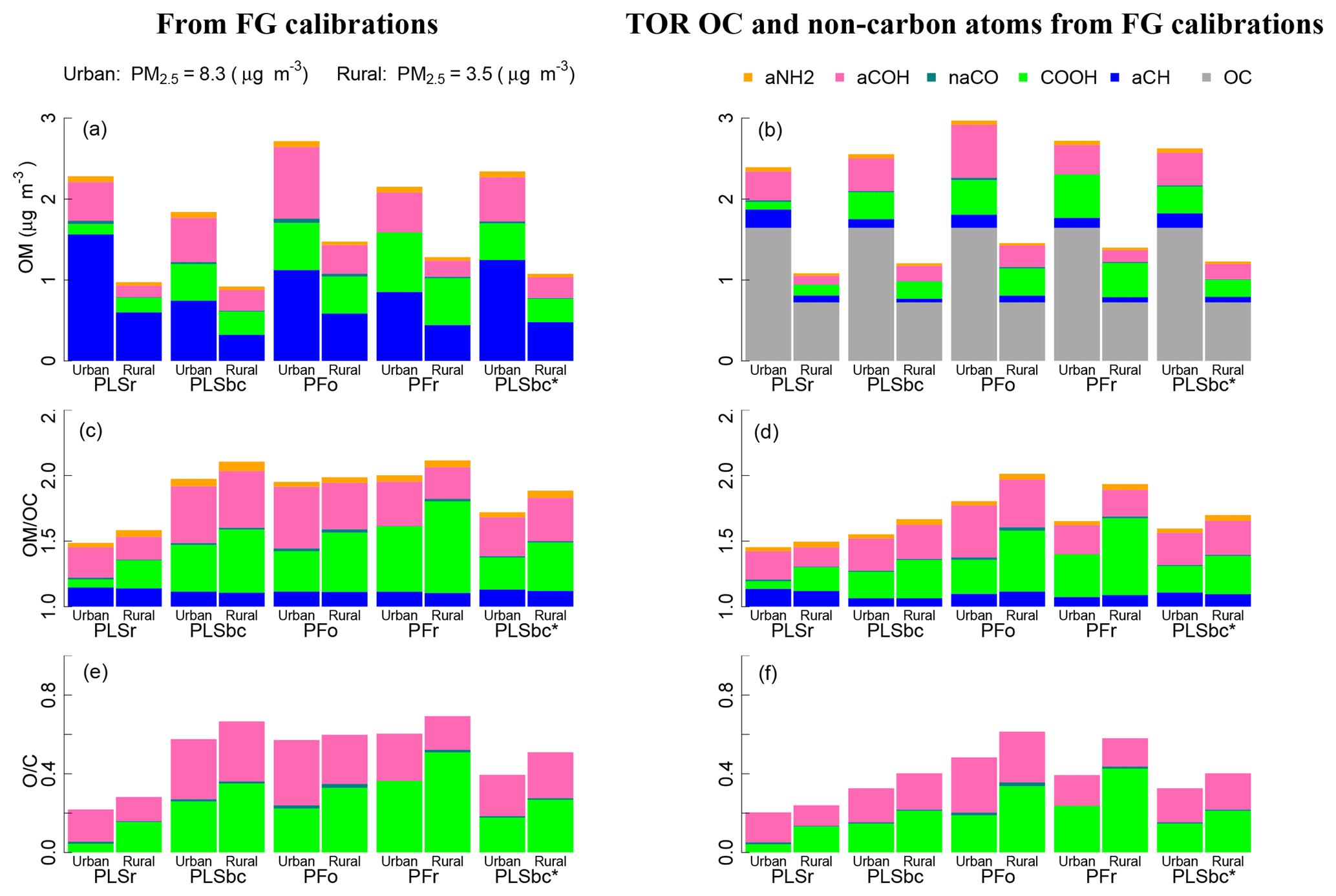
Figure 10(a, b) bar plots of OM mass fractions from quantified FGs. (c, d) bar plots of OM∕OC ratio and associated non-carbon atoms. (e, f) O∕C. In the left panels (a), (c), and (e) OM, OM∕OC and O∕C ratios use OC estimated by FG calibrations (FG OC). In the right panels (b), (d), and (f) the OM, OM∕OC and O∕C ratios use OC measured by TOR. PLSr and PLSbc refer to partial least square using raw and baseline-corrected spectra respectively. PFo and PFr refers to peak fitting using the original recalibrated absorption coefficients. PLSbc* is the same as PLSbc except that the number of LVs for aCH has been selected heuristically (Sect. 3.2).
The absolute magnitudes, however, require further consideration. The mean OM∕OC values estimated by PLSr (Ruthenburg et al., 2014) of 1.5 and 1.6 for urban and rural sites, respectively, are within range of values previously reported by GC-MS and AMS (Turpin and Lim, 2001; Aiken et al., 2008). However, the mean O∕C ratio of 0.25 for rural sites is particularly low and corresponds to values for hydrocarbon-like components derived from AMS PMF analysis (e.g., Aiken et al., 2008; de Gouw et al., 2009; Canagaratna et al., 2015). These results suggest that PLSr may be underestimating the oxygenated FGs (COOH and aCOH), especially for rural sites. The mean OM∕OC ratios for PLSbc, PFo and PFr are higher than PLSr and range from 2.0 (urban) up to 2.1 (rural), with O∕C ratios from 0.5 (urban) and 0.7 (rural). The surprisingly high values of OM∕OC and O∕C for urban samples can be attributed to an underestimation of FG OC, which inflates the OM∕OC estimates. However, the mass fractions of FGs (shown as conventional pie graphs in Fig. S10 in the Supplement) suggest relative proportions estimated by PFo, PFr, and PLSbc are similar to urban aerosol composition previously reported by Russell and co-workers (Russell et al., 2011; Takahama et al., 2013a). The proportion of aCH mass is estimated above 40 % and COOH and aCOH approximately one-quarter each; primary amine and carbonyl comprise the rest of the average OM mass for the urban samples (between 3 % and 6 %). In contrast, PLSr estimates the aCH fraction to be 71 % for urban samples and 64 % for rural (whereas the other models estimate between 35 % and 40 % for rural sites).
To improve these carbon-normalized metrics, the undetected carbon moieties can be corrected by incorporating an assumed carbon mass recovery fraction (Takahama and Ruggeri, 2017). Alternatively, an available OC reference measurement can instead be used for normalization – this can be TOR OC, which we use here, or TOR-equivalent OC estimated from FTIR spectra (Dillner and Takahama, 2015a; Reggente et al., 2016). This latter procedure leaves FTIR FG measurements to provide only the non-carbon atom content, which can be estimated with less uncertainty than the carbon content by using FG analysis (Sect. 2.6). The uncertainty in aCH abundance plays a critical role in estimation of carbon and OM mass, as nearly half of the total carbon is attributed to that associated with aCH. When using FG OC for normalization, contribution of this FG to the non-carbon portion of OM∕OC is 0.17 at most (Sect. S2), but this belies the substantial role in governing the overall magnitude of the ratio through its contribution to the OC estimate. However, if an external OC value is provided, the non-carbon contribution of aCH to OM is due to only hydrogen and the OM∕OC (and O∕C) is primarily dependent on estimates of the oxygenated fraction.
Figure 10 (right column) summarizes estimates of OM, OM∕OC, and O∕C obtained by using FTIR estimates for non-carbon atom abundance, and TOR OC for carbon content. The adjustments reflect the extent of underestimation of TOR OC by each of the models, and, predictably, the PLSr mean rural OM∕OC is reduced with respect to its urban counterpart while the mean urban OM∕OC is reduced with respect to the rural counterparts for the rest of the models. In the case of urban samples, the mean OM∕OC varies between 1.5 (PLSr) and 1.8 (PFo), and the mean O∕C varies between 0.20 (PLSr) and 0.48 (PFo). In the case of rural samples, the mean OM∕OC varies between 1.5 (PLSr) and 2.0 (PFo), and the mean O∕C varies between 0.21 (PLSr) and 0.61 (PFr).
When we heuristically adjust the PLSbc aCH model parameters to match TOR OC concentrations within 10 % on average (PLSbc* introduced in Sect. 3.2), estimated OM, OM∕OC, and O∕C values fall within the extremes spanned by the various models. While laboratory calibrations can generate models that give reasonable predictions for ambient samples (to the extent that they can be evaluated), this comparison underscores the challenge in selecting the most appropriate model for ambient samples based on laboratory data. More experience in evaluating different model selection criterion on extrapolation is necessary to improve the calibration strategy for FG estimation.
3.6 Anomalous samples
We examine and summarize in Fig. 11 a few of the anomalous clusters. Cluster 7 (first row in Fig. 11) samples have significant overprediction in both OC and ammonium for the calibration model using raw spectra (PLSr) but less in the baseline-corrected models. These samples are found in almost all sites and are primarily influenced by dust (Kuzmiakova, 2019). This conclusion is evidenced by the FTIR spectra having two sharp peaks above 3000 cm−1 and a broader peak between 950 and 1100 cm−1 indicative of Si–O bonds; resemblance of spectral features to hydroxyl groups from organic compounds or bound water in hydrates associated with dust is also observed. Accompanying XRF measurements also indicate high abundance of mineral dust elements in these samples. Larger atmospheric particles are likely to scatter infrared radiation, with increasing contributions above ∼200 nm (Signorell and Reid, 2010), and non-negligible contributions above 1 µm (Allen and Palen, 1989). While the primary purpose of the baseline correction is to remove the scattering from the PTFE fibers, it is also likely that there is a scattering contribution from the particles, which confers a positive artifact to the estimate of OC in the raw spectra calibration model. Baseline correction appears to reduce these artifacts through the removal of the particle scattering contribution to the observed absorbance.
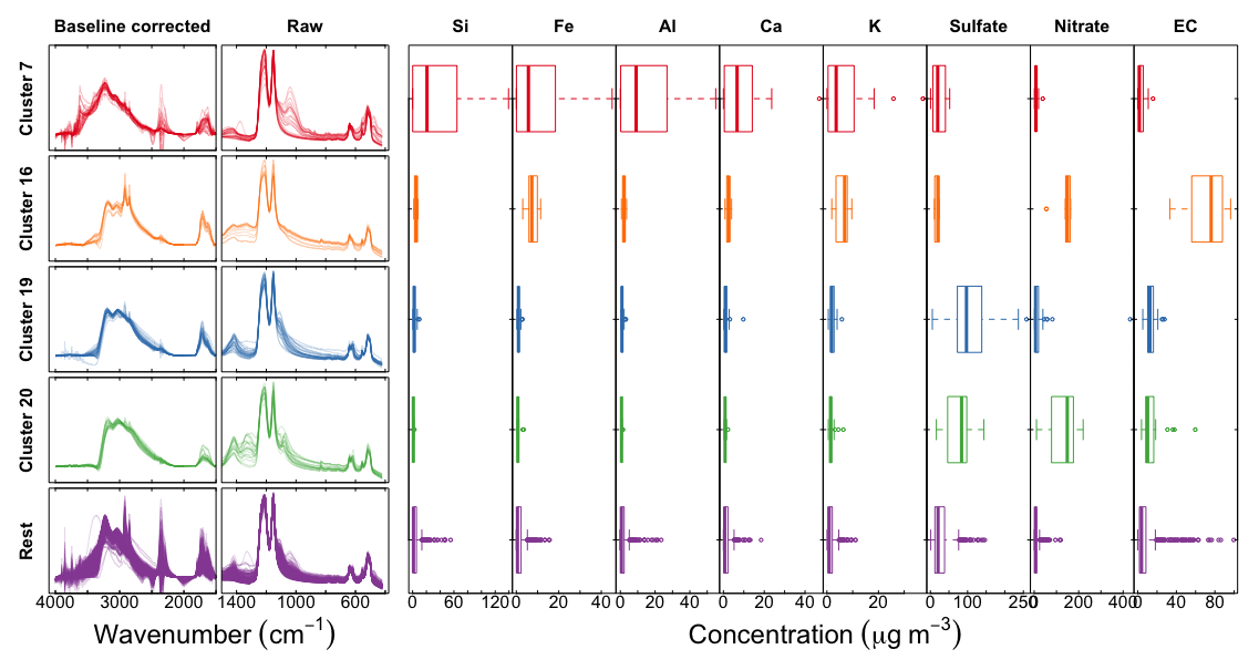
Figure 11Left column shows scaled baseline-corrected spectra between 4000 and 1500 cm−1; middle column shows scaled raw spectra below 1500 cm−1, and concentrations of PM constituents measured in the IMPROVE network: trace elements from X-ray fluorescence, inorganic ions (sulfate and nitrate) from ion chromatography, and elemental carbon from TOR analysis.
Cluster 16 (second row in Fig. 11) consists of wintertime Phoenix, AZ, samples which are associated with residential wood burning (Kuzmiakova, 2019). The consistent disagreement of the reference ammonium concentrations with all models suggests that the error may be attributed to the estimation of reference values rather than the calibrations. We expect gas–particle partitioning to favor the condensed phase for ammonium nitrate for wintertime temperatures in Phoenix, so an evaporation artifact from Teflon is not anticipated to be the most significant factor. However, potassium nitrate is a well-known product of biomass burning, and the offset in ammonium equivalently formulated in the magnitude of potassium matches the reported concentrations by XRF.
The atypical predictions for clusters 19 and 20 (third and fourth row in Fig. 11) are likely due to the abundance of large ammonium sulfate (cluster 19) and ammonium nitrate (cluster 20) particles in the samples, leading to anomalous transmission of infrared radiation (Christiansen peak effect) (Christiansen, 1885; Barnes and Bonner, 1936; Henry, 1948; Prost, 1973) through the sample (Fig. S15). The Christiansen peak effect occurs under two limiting conditions: the refractive index approaches that of the surrounding medium (air in this case), and the size of the particle(s) approaches the wavelength of the incident radiation. The refractive indices of ammonium sulfate and ammonium nitrate both exhibit a local minimum below 1.3 at 3.0 µm (3300 cm−1) (Jarzembski et al., 2003). PM2.5 can include some particles above 2.5 µm as the cut point corresponds to the median diameter of any particle efficiency curve of a size-selective inlet (cyclone for IMPROVE samples). However, another reason that the Christiansen effect plays a role in these samples is that its magnitude can still be significant for particles smaller than this diameter (Carlon, 1979). The result of this phenomenon is that the transmittance increases near this wavelength, though never approaching 100 % on account of co-absorbing substances and inhomogeneities in atmospheric particles (Shelyubskii, 1993; Pollard et al., 2007). The corresponding absorbance spectrum displays a sharp decrease at the Christiansen wavelength relative to its neighboring absorbances and spectral distortions in its vicinity. This optical artifact can affect both baseline correction and direct calibration (without baseline correction) if these effects are not taken into account, and our unexpected predictions can most certainly be attributed to this phenomenon. Remedies for this artifact may entail explicit modeling of the anomalous transmittance peak in the baseline correction or inclusion of samples which have this effect in the calibration samples. As both of these effects are nonlinear to absorbance, their treatment by a linear model may lead to a suboptimal representation of their contributions across multiple latent variables (including cross-over with contributions to the signal such as instrument noise; Zupan and Gasteiger, 1991). Nonetheless, the demonstrated performance of calibration models for TOR-equivalent OC prepared from the regression of FTIR spectra to collocated TOR OC measurements (Dillner and Takahama, 2015a) suggests that PLS can handle these irregularities (scattering, Christiansen effect) as long as samples which exhibit them are included in the calibration samples, with or without baseline correction.
In this work, we explore the diversity in FG predictions that can result from calibration models built with mid-IR spectra. In particular, we compare two prominent methods for estimation of functional groups (FGs) from mid-IR spectra used in atmospheric PM analysis: peak fitting (PF) and partial least squares (PLS) regression. PF is an approach using physically based absorption profiles to model spectral signals, and PLS is a statistical approach which is trained on relevant features from reference spectra. Using PF, we evaluated FG estimates using molar absorbance coefficients (model parameters) from previous studies (PFo) and calculated (PFr) using 238 laboratory standards from Ruthenburg et al. (2014). Using PLS, we evaluated FG estimations using raw spectra (PLSr, in which substrate PTFE interferences are present) and baseline-corrected spectra (PLSbc).
PFo and PFr require some assumptions: (i) structure of the PTFE signal; (ii) value of the molar absorbance coefficients; and (iii) apportionment rule to apportion carbonyl to carboxylic and non-acid contributions. Underestimation of OC in comparison to TOR (by as much as 50 %) and surprisingly high values of OM∕OC (greater than 1.8) for the urban site, Phoenix, is likely due to the underestimation of aCH. Using a different value of the absorption coefficient, particularly for aCH, within uncertainty bounds presented in this study can mitigate this discrepancy.
PLSr requires the least prior knowledge – e.g., how to model the baseline – and therefore brings an appealing approach to calibration. However, scattering contributions from larger ambient particles can lead to overprediction of organic FGs and ammonium in ambient samples with considerable dust impacts. As reported in previous studies (Ruthenburg et al., 2014; Takahama and Dillner, 2015) PLSr shows good agreement (correlation coefficients above 0.85 and regression slope close to 0.9) with external TOR OC measurements, especially for urban samples, and the OM∕OC values are also within range of expected values (1.4–1.8). However, the higher values of OM∕OC at the rural sites may be due to an underestimation of the oxygenated FGs, which leads to a lower estimate of carbon content and an artificial increase the OM∕OC. This bias is apparent when normalizing by TOR OC, as the OM∕OC ratios of rural sites become similar to the urban values. PLSbc reveals the most consistent estimates against PFr, and this is sensible as the two use the closest correspondence of laboratory standards and spectral preparation (baseline correction).
Both PLSbc and PLSr can quantify carboxylic acid and non-acid carbonyl groups directly by designating the target variable to COOH and naCO, and the models are trained on wavenumbers and LVs relevant for the two species. From this analysis, we conclude that almost all of the carbonyl for samples in the seven 2011 IMPROVE sites is associated with carboxylic rather than ketone or ester CO. In principle, it is also possible to define a fixed relationship between carboxylic cCOH and carbonyl CO such that COOH and the residual naCO can be determined in PF, but this requires additional assumptions to implement.
In summary, models built with laboratory standards and algorithms are able to extract relevant information from ambient FTIR sample spectra. Evaluation against external reference values (TOR OC and ammonium estimated from anion chromatography analysis) suggests moderately strong to strong correlation for this IMPROVE monitoring data set, and it is generally consistent with past studies that have also found high correlation with collocated measurements of TOR OC and AMS OM (e.g., Russell et al., 2009a; Gilardoni et al., 2009; Takahama and Russell, 2011; Corrigan et al., 2013). However, the overall magnitude of bias can vary substantially depending on the choice of models and parameters. While we should also not expect perfect agreement as each of the external measurements has its own artifacts, the sensitivity and resulting uncertainty in FG estimation due to available selection of parameters is apparent. Many parameters give validated predictions for laboratory standards, but each can give different results when applied to ambient samples (i.e., estimating concentrations in ambient samples is an ill-posed problem). Use of different absorption coefficients for PF and number of LVs for PLS that are still consistent within limits of the calibration standards in this work can offset apparent biases, but there are many parameters and their selection criteria are presently not sufficiently constrained. An example was shown where the overall magnitude in estimated FTIR OC can vary by 40 % (and effectively eliminating bias with respect to TOR OC) by adjusting the number of LVs for aCH used by the PLSbc model.
Reducing uncertainty in predictions derived from FTIR spectra can be envisioned by two means: further advancing our study of laboratory standards that mimic ambient samples more closely and by exploring mathematical solutions possible within a stricter set of constraints. Regarding the first point, Takahama et al. (2016) note that predictions from statistical calibration models (PLS and its variants) become less sensitive to model parameters as the samples in the calibration and prediction sets become more similar, and presumably this conclusion can be extended to the PF approach in its use of absorption profiles (both in intensity and shape).
Given that some differences will remain between key features in laboratory standards and ambient samples, the second point on algorithmic improvements can be formulated in several ways. One strategy is to explore the subset of solutions that are consistent with available external measurements (e.g., TOR OC, AMS OM, and other chemical information) to revise model selection criteria. While an example varying the number of LVs for aCH is shown in this work, a more formal approach to multi-parameter optimization is preferable for approaching this task. Targeting means to establish different relationships between spectra and FGs than considered in this work is also possible. For instance, the full range of available calibration samples or absorption coefficients are likely not the most appropriate for every sample. Diversity in sample composition – e.g., between urban and rural samples – can be incorporated in a multilevel modeling approach, whereby different model or model parameters can be used based on spectral shape or identified source contributions (e.g., using positive matrix factorization; Paatero and Tapper, 1994). Furthermore, models can be constrained to share a common representation to follow actual structure–spectra correlations more closely than when models for each FG are constructed independently – i.e., constraints on the internal representation of interferences toward organic FG quantification can be improved by concurrently developing our capability to model ammonium nitrate and ammonium sulfate using their discriminating bands. The same parameters (either absorption profiles in PF or LVs in PLS) that are able to accurately predict concentrations of these inorganic compounds would likely be able to model their interferences to organic FG absorption more correctly over a broader range of instances.
Finally, anticipating the mass fraction of OC that can be explained by FGs will continue to play an important role in estimating the overall OM, particularly for the OM∕OC ratio. There are few classes of carbon atoms in molecules that are not expected to be detected by FTIR (i.e., they are not associated with FGs for which calibrations are not built), and understanding the expected extent of underestimation of OC by FG reconstruction will provide better perspective on evaluation of FG OC by TOR OC and model selection methods. While the specific molecules in the aerosol mixture need not be enumerated for this purpose, the knowledge of the functionalized carbon types that are present in different sample types – which can be obtained through measurements and simulation (Takahama and Ruggeri, 2017) – is useful in this regard. In the meantime, continuing improvement in estimation of TOR-equivalent OC from direct calibration to collocated measurements (Dillner and Takahama, 2015a; Weakley et al., 2016) can enable estimation of carbon content from the same FTIR spectrum without imposing uncertainty from FG calibrations or requiring collocated TOR measurements.
FTIR spectroscopy remains a promising analytical technique to provide independent estimates of OM, OM∕OC, and O∕C based on molecular structure. Presently, a large number of calibration models can be generated based on selection of laboratory standards and algorithms, but further research is needed to develop a robust model selection process to reduce uncertainty in prediction when applied to ambient samples. Users should therefore note the existence of potential biases in current FTIR calibration models due to model or parameter sensitivity when performing comparisons against external measurements. However, further progress is being made toward development of calibration strategies.
Baseline correction (Kuzmiakova et al., 2016), Peak fitting (Takahama et al., 2013b) and multivariate calibration (Dillner and Takahama, 2015a, b) are implemented in an open platform with browser interface, accessible at http://airspec.epfl.ch (last access: 4 April 2019). Access to the software and their repositories are described in the companion paper (Reggente et al., 2019).
The IMPROVE network spectra will be made publicly available. TOR OC and PM2.5 can be downloaded from the US Federal Land Manager Environmental Database at http://views.cira.colostate.edu/fed/QueryWizard/Default.aspx (last access: 4 April 2019).
Table A1 includes pervasive abbreviations used in multiple sections.
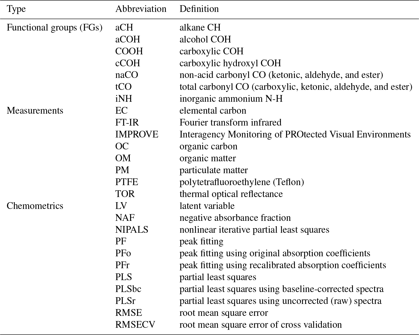
The supplement related to this article is available online at: https://doi.org/10.5194/amt-12-2287-2019-supplement.
MR and ST have performed the analysis, written the manuscript, and prepared the artwork. AD has provided the sample spectra and contributed in writing and revising the manuscript.
The authors declare that they have no conflict of interest.
The authors acknowledge funding from EPFL and the IMPROVE program with support from the US Environmental Protection Agency (National Park Service cooperative agreement Pl8AC01222). We also thank Christophe Delval for assistance in identification of the Christiansen peak species.
This paper was edited by Charles Brock and reviewed by two anonymous referees.
Aiken, A. C., Decarlo, P. F., Kroll, J. H., Worsnop, D. R., Huffman, J. A., Docherty, K. S., Ulbrich, I. M., Mohr, C., Kimmel, J. R., Sueper, D., Sun, Y., Zhang, Q., Trimborn, A., Northway, M., Ziemann, P. J., Canagaratna, M. R., Onasch, T. B., Alfarra, M. R., Prevot, A. S. H., Dommen, J., Duplissy, J., Metzger, A., Baltensperger, U., and Jimenez, J. L.: O∕C and OM∕OC ratios of primary, secondary, and ambient organic aerosols with high-resolution time-of-flight aerosol mass spectrometry, Environ. Sci. Technol., 42, 4478–4485, https://doi.org/10.1021/es703009q, 2008. a, b, c
Allen, D. T. and Palen, E.: Recent advances in aerosol analysis by infrared spectroscopy, J. Aerosol Sci., 20, 441–455, https://doi.org/10.1016/0021-8502(89)90078-5, 1989. a, b
Allen, D. T., Palen, E. J., Haimov, M. I., Hering, S. V., and Young, J. R.: Fourier-transform Infrared-spectroscopy of Aerosol Collected In A Low-pressure Impactor (LPI/FTIR) – Method Development and Field Calibration, Aerosol Sci. Technol., 21, 325–342, https://doi.org/10.1080/02786829408959719, 1994. a, b
Alsberg, B. K., Winson, M. K., and Kell, D. B.: Improving the interpretation of multivariate and rule induction models by using a peak parameter representation, Chemometr. Intell. Lab., 36, 95–109, https://doi.org/10.1016/S0169-7439(97)00024-5, 1997. a
Arlot, S. and Celisse, A.: A survey of cross-validation procedures for model selection, Stat. Surv., 4, 40–79, https://doi.org/10.1214/09-SS054, 2010. a
Atkins, P. and de Paula, J.: Physical Chemistry, W. H. Freeman and Company, New York, 2006. a
Ayres, B. R., Allen, H. M., Draper, D. C., Brown, S. S., Wild, R. J., Jimenez, J. L., Day, D. A., Campuzano-Jost, P., Hu, W., de Gouw, J., Koss, A., Cohen, R. C., Duffey, K. C., Romer, P., Baumann, K., Edgerton, E., Takahama, S., Thornton, J. A., Lee, B. H., Lopez-Hilfiker, F. D., Mohr, C., Wennberg, P. O., Nguyen, T. B., Teng, A., Goldstein, A. H., Olson, K., and Fry, J. L.: Organic nitrate aerosol formation via NO3 + biogenic volatile organic compounds in the southeastern United States, Atmos. Chem. Phys., 15, 13377–13392, https://doi.org/10.5194/acp-15-13377-2015, 2015. a
Barnes, R. B. and Bonner, L. G.: The Christiansen Filter Effect in the Infrared, Phys. Rev., 49, 732–740, https://doi.org/10.1103/PhysRev.49.732, 1936. a
Blando, J. D., Porcja, R. J., Li, T. H., Bowman, D., Lioy, P. J., and Turpin, B. J.: Secondary formation and the Smoky Mountain organic aerosol: An examination of aerosol polarity and functional group composition during SEAVS RID F-6148-2011, Environ. Sci. Technol., 32, 604–613, https://doi.org/10.1021/es970405s, 1998. a
Canagaratna, M. R., Jimenez, J. L., Kroll, J. H., Chen, Q., Kessler, S. H., Massoli, P., Hildebrandt Ruiz, L., Fortner, E., Williams, L. R., Wilson, K. R., Surratt, J. D., Donahue, N. M., Jayne, J. T., and Worsnop, D. R.: Elemental ratio measurements of organic compounds using aerosol mass spectrometry: characterization, improved calibration, and implications, Atmos. Chem. Phys., 15, 253–272, https://doi.org/10.5194/acp-15-253-2015, 2015. a
Carlon, H. R.: Christiansen effect in IR spectra of soil-derived atmospheric dusts, Appl. Opt., 18, 3610–3614, https://doi.org/10.1364/AO.18.003610, 1979. a
Chen, Q., Ikemori, F., Higo, H., Asakawa, D., and Mochida, M.: Chemical Structural Characteristics of HULIS and Other Fractionated Organic Matter in Urban Aerosols: Results from Mass Spectral and FT-IR Analysis, Environ. Sci. Technol., 50, 1721–1730, https://doi.org/10.1021/acs.est.5b05277, 2016. a
Chhabra, P. S., Ng, N. L., Canagaratna, M. R., Corrigan, A. L., Russell, L. M., Worsnop, D. R., Flagan, R. C., and Seinfeld, J. H.: Elemental composition and oxidation of chamber organic aerosol, Atmos. Chem. Phys., 11, 8827–8845, https://doi.org/10.5194/acp-11-8827-2011, 2011. a
Chow, J. C., Watson, J. G., Pritchett, L. C., Pierson, W. R., Frazier, C. A., and Purcell, R. G.: The dri thermal/optical reflectance carbon analysis system: description, evaluation and applications in U.S. Air quality studies, Atmos. Environ., 27, 1185–1201, https://doi.org/10.1016/0960-1686(93)90245-T, 1993. a
Chow, J. C., Watson, J. G., Chen, L.-W. A., Chang, M. O., Robinson, N. F., Trimble, D., and Kohl, S.: The IMPROVE_A Temperature Protocol for Thermal/Optical Carbon Analysis: Maintaining Consistency with a Long-Term Database, J. Air Waste Manage. Assoc., 57, 1014–1023, https://doi.org/10.3155/1047-3289.57.9.1014, 2007. a
Christiansen, C.: Untersuchungen über die optischen Eigenschaften von fein vertheilten Körpern, Ann. Phys.-Berlin, 260, 439–446, https://doi.org/10.1002/andp.18852600305, 1885. a
Corrigan, A. L., Russell, L. M., Takahama, S., Äijälä, M., Ehn, M., Junninen, H., Rinne, J., Petäjä, T., Kulmala, M., Vogel, A. L., Hoffmann, T., Ebben, C. J., Geiger, F. M., Chhabra, P., Seinfeld, J. H., Worsnop, D. R., Song, W., Auld, J., and Williams, J.: Biogenic and biomass burning organic aerosol in a boreal forest at Hyytiälä, Finland, during HUMPPA-COPEC 2010, Atmos. Chem. Phys., 13, 12233–12256, https://doi.org/10.5194/acp-13-12233-2013, 2013. a, b, c
Coury, C. and Dillner, A. M.: A method to quantify organic functional groups and inorganic compounds in ambient aerosols using attenuated total reflectance FTIR spectroscopy and multivariate chemometric techniques, Atmos. Environ., 42, 5923–5932, https://doi.org/10.1016/j.atmosenv.2008.03.026, 2008. a
Craig, R. L., Bondy, A. L., and Ault, A. P.: Surface Enhanced Raman Spectroscopy Enables Observations of Previously Undetectable Secondary Organic Aerosol Components at the Individual Particle Level, Anal. Chem., 87, 7510–7514, https://doi.org/10.1021/acs.analchem.5b01507, 2015. a
Cunningham, P. T., Johnson, S. A., and Yang, R. T.: Variations in chemistry of airborne particulate material with particle size and time, Environ. Sci. Technol., 8, 131–135, https://doi.org/10.1021/es60087a002, 1974. a
Day, D. A., Liu, S., Russell, L. M., and Ziemann, P. J.: Organonitrate group concentrations in submicron particles with high nitrate and organic fractions in coastal southern California, Atmos. Environ., 44, 1970–1979, https://doi.org/10.1016/j.atmosenv.2010.02.045, 2010. a
Decesari, S., Mircea, M., Cavalli, F., Fuzzi, S., Moretti, F., Tagliavini, E., and Facchini, M. C.: Source attribution of water-soluble organic aerosol by nuclear magnetic resonance spectroscopy, Environ. Sci. Technol., 41, 2479–2484, https://doi.org/10.1021/es061711l, 2007. a, b
de Gouw, J. A., Welsh-Bon, D., Warneke, C., Kuster, W. C., Alexander, L., Baker, A. K., Beyersdorf, A. J., Blake, D. R., Canagaratna, M., Celada, A. T., Huey, L. G., Junkermann, W., Onasch, T. B., Salcido, A., Sjostedt, S. J., Sullivan, A. P., Tanner, D. J., Vargas, O., Weber, R. J., Worsnop, D. R., Yu, X. Y., and Zaveri, R.: Emission and chemistry of organic carbon in the gas and aerosol phase at a sub-urban site near Mexico City in March 2006 during the MILAGRO study, Atmos. Chem. Phys., 9, 3425–3442, https://doi.org/10.5194/acp-9-3425-2009, 2009. a
Dillner, A. M. and Takahama, S.: Predicting ambient aerosol thermal-optical reflectance (TOR) measurements from infrared spectra: organic carbon, Atmos. Meas. Tech., 8, 1097–1109, https://doi.org/10.5194/amt-8-1097-2015, 2015a. a, b, c, d, e, f
Dillner, A. M. and Takahama, S.: Predicting ambient aerosol thermal-optical reflectance measurements from infrared spectra: elemental carbon, Atmos. Meas. Tech., 8, 4013–4023, https://doi.org/10.5194/amt-8-4013-2015, 2015b. a, b
Dron, J., El Haddad, I., Temime-Roussel, B., Jaffrezo, J.-L., Wortham, H., and Marchand, N.: Functional group composition of ambient and source organic aerosols determined by tandem mass spectrometry, Atmos. Chem. Phys., 10, 7041–7055, https://doi.org/10.5194/acp-10-7041-2010, 2010. a
Duyckaerts, G.: The infra-red analysis of solid substances, A review, Analyst, 84, 201–214, https://doi.org/10.1039/AN9598400201, 1959. a
Faber, P., Drewnick, F., Bierl, R., and Borrmann, S.: Complementary online aerosol mass spectrometry and offline FT-IR spectroscopy measurements: Prospects and challenges for the analysis of anthropogenic aerosol particle emissions, Atmos. Environ., 166, 92–98, https://doi.org/10.1016/j.atmosenv.2017.07.014, 2017. a
Fry, J. L., Draper, D. C., Zarzana, K. J., Campuzano-Jost, P., Day, D. A., Jimenez, J. L., Brown, S. S., Cohen, R. C., Kaser, L., Hansel, A., Cappellin, L., Karl, T., Hodzic Roux, A., Turnipseed, A., Cantrell, C., Lefer, B. L., and Grossberg, N.: Observations of gas- and aerosol-phase organic nitrates at BEACHON-RoMBAS 2011, Atmos. Chem. Phys., 13, 8585–8605, https://doi.org/10.5194/acp-13-8585-2013, 2013. a
Fu, D., Leng, C., Kelley, J., Zeng, G., Zhang, Y., and Liu, Y.: ATR-IR Study of Ozone Initiated Heterogeneous Oxidation of Squalene in an Indoor Environment, Environ. Sci. Technol., 47, 10611–10618, https://doi.org/10.1021/es4019018, 2013. a
Geladi, P. and Kowalski, B. R.: Partial least-squares regression: a tutorial, Anal. Chim. Acta, 185, 1–17, https://doi.org/10.1016/0003-2670(86)80028-9, 1986. a
Gilardoni, S., Russell, L. M., Sorooshian, A., Flagan, R. C., Seinfeld, J. H., Bates, T. S., Quinn, P. K., Allan, J. D., Williams, B., Goldstein, A. H., Onasch, T. B., and Worsnop, D. R.: Regional variation of organic functional groups in aerosol particles on four US east coast platforms during the International Consortium for Atmospheric Research on Transport and Transformation 2004 campaign, J. Geophys. Res.-Atmos., 112, D10S27, https://doi.org/10.1029/2006JD007737, 2007. a, b, c, d, e, f, g
Gilardoni, S., Liu, S., Takahama, S., Russell, L. M., Allan, J. D., Steinbrecher, R., Jimenez, J. L., De Carlo, P. F., Dunlea, E. J., and Baumgardner, D.: Characterization of organic ambient aerosol during MIRAGE 2006 on three platforms, Atmos. Chem. Phys., 9, 5417–5432, https://doi.org/10.5194/acp-9-5417-2009, 2009. a
Gowen, A. A., Downey, G., Esquerre, C., and O'Donnell, C. P.: Preventing over-fitting in PLS calibration models of near-infrared (NIR) spectroscopy data using regression coefficients, J. Chemometr., 25, 375–381, https://doi.org/10.1002/cem.1349, 2011. a
Griffiths, P. and Haseth, J. A. D.: Fourier Transform Infrared Spectrometry, 2nd edn., John Wiley & Sons, Hoboken, New Jersey, 2007. a, b
Haaland, D. M. and Thomas, E. V.: Partial least-squares methods for spectral analyses. 1. Relation to other quantitative calibration methods and the extraction of qualitative information, Anal. Chem., 60, 1193–1202, https://doi.org/10.1021/ac00162a020, 1988. a, b
Hallquist, M., Wenger, J. C., Baltensperger, U., Rudich, Y., Simpson, D., Claeys, M., Dommen, J., Donahue, N. M., George, C., Goldstein, A. H., Hamilton, J. F., Herrmann, H., Hoffmann, T., Iinuma, Y., Jang, M., Jenkin, M. E., Jimenez, J. L., Kiendler-Scharr, A., Maenhaut, W., McFiggans, G., Mentel, Th. F., Monod, A., Prévôt, A. S. H., Seinfeld, J. H., Surratt, J. D., Szmigielski, R., and Wildt, J.: The formation, properties and impact of secondary organic aerosol: current and emerging issues, Atmos. Chem. Phys., 9, 5155–5236, https://doi.org/10.5194/acp-9-5155-2009, 2009. a
Hamilton, J. F., Webb, P. J., Lewis, A. C., Hopkins, J. R., Smith, S., and Davy, P.: Partially oxidised organic components in urban aerosol using GCXGC-TOF/MS, Atmos. Chem. Phys., 4, 1279–1290, https://doi.org/10.5194/acp-4-1279-2004, 2004. a
Harris, D. C. and Bertolucci, M. D.: Symmetry and Spectroscopy: An Introduction to Vibrational and Electronic Spectroscopy, Dover Publications, New York, 1989. a
Hasegawa, T.: Quantitative Infrared Spectroscopy for Understanding of a Condensed Matter, https://doi.org/10.1007/978-4-431-56493-5, Springer, Japan, 2017. a
Hastie, T., Tibshirani, R., and Friedman, J.: The elements of statistical learning: data mining, inference, and prediction, Springer Verlag, New York, 2009. a
Hawkins, L. N. and Russell, L. M.: Oxidation of ketone groups in transported biomass burning aerosol from the 2008 Northern California Lightning Series fires, Atmos. Environ., 44, 4142–4154, https://doi.org/10.1016/j.atmosenv.2010.07.036, 2010. a
Henry, R. L.: The Transmission of Powder Films in the Infra-Red, J. Opt. Soc. Am., 38, 775–789, https://doi.org/10.1364/JOSA.38.000775, 1948. a
Hung, H.-M., Katrib, Y., and Martin, S. T.: Products and Mechanisms of the Reaction of Oleic Acid with Ozone and Nitrate Radical, J. Phys. Chem. A, 109, 4517–4530, https://doi.org/10.1021/jp0500900, 2005. a
Jarzembski, M. A., Norman, M. L., Fuller, K. A., Srivastava, V., and Cutten, D. R.: Complex refractive index of ammonium nitrate in the 2–20 µm spectral range, Appl. Opt., 42, 922–930, https://doi.org/10.1364/AO.42.000922, 2003. a
Jenkin, M. E., Saunders, S. M., and Pilling, M. J.: The tropospheric degradation of volatile organic compounds: a protocol for mechanism development, Atmos. Environ., 31, 81–104, https://doi.org/10.1016/S1352-2310(96)00105-7, 1997. a
Johnson, S. A., Graczyk, D. G., Kumar, R., and Cunningham, P. T.: Analytical Techniques for Ambient Sulfate Aerosols, Tech. Rep. ANL-81-12, http://www.osti.gov/scitech/biblio/6515722 (last access: 4 April 2019), Argonne National Lab, IL (USA), 1981. a
Kalafut-Pettibone, A. J. and McGivern, W. S.: Analytical Methodology for Determination of Organic Aerosol Functional Group Distributions, Anal. Chem., 85, 3553–3560, https://doi.org/10.1021/ac3028728, 2013. a
Kamruzzaman, M., Takahama, S., and Dillner, A. M.: Quantification of amine functional groups and their influence on OM∕OC in the IMPROVE network, Atmos. Environ., 172, 124–132, https://doi.org/10.1016/j.atmosenv.2017.10.053, 2018. a
Kelley, A. M.: Condensed-Phase Molecular Spectroscopy and Photophysics, John Wiley & Sons, Hoboken, 2013. a
Kidd, C., Perraud, V., and Finlayson-Pitts, B. J.: New insights into secondary organic aerosol from the ozonolysis of α-pinene from combined infrared spectroscopy and mass spectrometry measurements, Phys. Chem. Chem. Phys., 16, 22706–22716, https://doi.org/10.1039/C4CP03405H, 2014. a
Kroll, J. H. and Seinfeld, J. H.: Chemistry of secondary organic aerosol: Formation and evolution of low-volatility organics in the atmosphere, Atmos. Environ., 42, 3593–3624, https://doi.org/10.1016/j.atmosenv.2008.01.003, 2008. a
Kroll, J. H., Donahue, N. M., Jimenez, J. L., Kessler, S. H., Canagaratna, M. R., Wilson, K. R., Altieri, K. E., Mazzoleni, L. R., Wozniak, A. S., Bluhm, H., Mysak, E. R., Smith, J. D., Kolb, C. E., and Worsnop, D. R.: Carbon oxidation state as a metric for describing the chemistry of atmospheric organic aerosol, Nat. Chem., 3, 133–139, https://doi.org/10.1038/nchem.948, 2011. a
Krost, K. J. and McClenny, W. A.: FT-IR Transmission Spectroscopy for Quantitation of Ammonium Bisulfate in Fine-Particulate Matter Collected on Teflon Filters, Appl. Spectrosc., 48, 702–705, https://doi.org/10.1366/000370294774368983, 1994. a, b
Kulkarni, P., Baron, P. A., and Willeke, K.: Aerosol Measurement: Principles, Techniques, and Applications, John Wiley & Sons, Hoboken, 2011. a
Kuzmiakova, A., Dillner, A. M., and Takahama, S.: An automated baseline correction protocol for infrared spectra of atmospheric aerosols collected on polytetrafluoroethylene (Teflon) filters, Atmos. Meas. Tech., 9, 2615–2631, https://doi.org/10.5194/amt-9-2615-2016, 2016. a, b, c, d
Laskin, A., Laskin, J., and Nizkorodov, S. A.: Mass spectrometric approaches for chemical characterisation of atmospheric aerosols: critical review of the most recent advances, Environ. Chem., 9, 163–189, https://doi.org/10.1071/EN12052, 2012. a
Lim, H. J. and Turpin, B. J.: Origins of primary and secondary organic aerosol in Atlanta: Results' of time-resolved measurements during the Atlanta supersite experiment, Environ. Sci. Technol., 36, 4489–4496, https://doi.org/10.1021/es0206487, 2002. a
Lim, Y. B., Tan, Y., Perri, M. J., Seitzinger, S. P., and Turpin, B. J.: Aqueous chemistry and its role in secondary organic aerosol (SOA) formation, Atmos. Chem. Phys., 10, 10521–10539, https://doi.org/10.5194/acp-10-10521-2010, 2010. a
Liu, J.: Developing a soft sensor based on sparse partial least squares with variable selection, J. Process. Contr., 24, 1046–1056, https://doi.org/10.1016/j.jprocont.2014.05.014, 2014. a
Liu, S., Takahama, S., Russell, L. M., Gilardoni, S., and Baumgardner, D.: Oxygenated organic functional groups and their sources in single and submicron organic particles in MILAGRO 2006 campaign, Atmos. Chem. Phys., 9, 6849–6863, https://doi.org/10.5194/acp-9-6849-2009, 2009. a
Liu, S., Day, D. A., Shields, J. E., and Russell, L. M.: Ozone-driven daytime formation of secondary organic aerosol containing carboxylic acid groups and alkane groups, Atmos. Chem. Phys., 11, 8321–8341, https://doi.org/10.5194/acp-11-8321-2011, 2011. a, b
Liu, S., Ahlm, L., Day, D. A., Russell, L. M., Zhao, Y., Gentner, D. R., Weber, R. J., Goldstein, A. H., Jaoui, M., Offenberg, J. H., Kleindienst, T. E., Rubitschun, C., Surratt, J. D., Sheesley, R. J., and Scheller, S.: Secondary organic aerosol formation from fossil fuel sources contribute majority of summertime organic mass at Bakersfield, J. Geophys.-Res.-Atmos., 117, D00V26, https://doi.org/10.1029/2012JD018170, 2012. a
Liu, X., Martin-Calvo, A., McGarrity, E., Schnell, S. K., Calero, S., Simon, J.-M., Bedeaux, D., Kjelstrup, S., Bardow, A., and Vlugt, T. J. H.: Fick Diffusion Coefficients in Ternary Liquid Systems from Equilibrium Molecular Dynamics Simulations, Ind. Eng. Chem. Res., 51, 10247–10258, https://doi.org/10.1021/ie301009v, 2012. a
Mader, P. P., MacPhee, R. D., Lofberg, R. T., and Larson, G. P.: Composition of Organic Portion of Atmospheric Aerosols in the Los Angeles Area, Ind. Eng. Chem., 44, 1352–1355, https://doi.org/10.1021/ie50510a047, 1952. a
Maria, S. F., Russell, L. M., Turpin, B. J., and Porcja, R. J.: FTIR measurements of functional groups and organic mass in aerosol samples over the Caribbean, Atmos. Environ., 36, 5185–5196, https://doi.org/10.1016/S1352-2310(02)00654-4, 2002. a
Maria, S. F., Russell, L. M., Turpin, B. J., Porcja, R. J., Campos, T. L., Weber, R. J., and Huebert, B. J.: Source signatures of carbon monoxide and organic functional groups in Asian Pacific Regional Aerosol Characterization Experiment (ACE-Asia) submicron aerosol types, J. Geophys. Res.-Atmos., 108, 8637, https://doi.org/10.1029/2003JD003703, 2003. a, b, c, d, e
Martens, H. and Næs, T.: Multivariate Calibration, John Wiley & Sons, New York, 1991. a, b
Massart, D. L., Vandeginste, B. G. M., Deming, S. N., Michotte, Y., and Kaufman, L.: Chemometrics: A Textbook, Data Handling in Science and Technology, Elsevier Science, Amsterdam, 1988. a
McClenny, W. A., Childers, J. W., Rōhl, R., and Palmer, R. A.: FTIR transmission spectrometry for the nondestructive determination of ammonium and sulfate in ambient aerosols collected on teflon filters, Atmos. Environ., 19, 1891–1898, https://doi.org/10.1016/0004-6981(85)90014-9, 1985. a, b, c
Ng, N. L., Brown, S. S., Archibald, A. T., Atlas, E., Cohen, R. C., Crowley, J. N., Day, D. A., Donahue, N. M., Fry, J. L., Fuchs, H., Griffin, R. J., Guzman, M. I., Herrmann, H., Hodzic, A., Iinuma, Y., Jimenez, J. L., Kiendler-Scharr, A., Lee, B. H., Luecken, D. J., Mao, J., McLaren, R., Mutzel, A., Osthoff, H. D., Ouyang, B., Picquet-Varrault, B., Platt, U., Pye, H. O. T., Rudich, Y., Schwantes, R. H., Shiraiwa, M., Stutz, J., Thornton, J. A., Tilgner, A., Williams, B. J., and Zaveri, R. A.: Nitrate radicals and biogenic volatile organic compounds: oxidation, mechanisms, and organic aerosol, Atmos. Chem. Phys., 17, 2103–2162, https://doi.org/10.5194/acp-17-2103-2017, 2017. a
Nordlund, T. M.: Quantitative Understanding of Biosystems: An Introduction to Biophysics, CRC Press, Boca Raton, 2011. a
Paatero, P. and Tapper, U.: Positive Matrix Factorization – A Nonnegative Factor Model With Optimal Utilization of Error-estimates of Data Values, Environmetrics, 5, 111–126, 1994. a
Palen, E. J., Allen, D. T., Pandis, S. N., Paulson, S. E., Seinfeld, J. H., and Flagan, R. C.: Fourier-transform Infrared-analysis of Aerosol Formed In the Photooxidation of Isoprene and Beta-pinene, Atmos. Environ., 26, 1239–1251, https://doi.org/10.1016/0960-1686(92)90385-X, 1992. a
Pollard, M., Jaklevic, J., and Howes, J.: Fourier Transform Infrared and Ion-Chromatographic Sulfate Analysis of Ambient Air Samples, Aerosol Sci. Tech., 12, 105–113, https://doi.org/10.1080/02786829008959330, 1990. a
Pollard, M. J., Griffiths, P. R., and Nishikida, K.: Investigation of the Christiansen Effect in the Mid-Infrared Region for Airborne Particles, Appl. Spectrosc., 61, 860–866, https://doi.org/10.1366/000370207781540123, 2007. a
Presto, A. A., Hartz, K. E. H., and Donahue, N. M.: Secondary organic aerosol production from terpene ozonolysis, 2, Effect of NOx concentration, Environ. Sci. Technol., 39, 7046–7054, https://doi.org/10.1021/es050400s, 2005. a
Prost, R.: The influence of the Christiansen effect on IR spectra of powders, Clay. Clay Miner., 21, 363–368, 1973. a
Ranney, A. P. and Ziemann, P. J.: Microscale spectrophotometric methods for quantification of functional groups in oxidized organic aerosol, Aerosol Scie. Tech., 50, 881–892, https://doi.org/10.1080/02786826.2016.1201197, 2016. a
Reff, A., Turpin, B. J., Offenberg, J. H., Weisel, C. P., Zhang, J., Morandi, M., Stock, T., Colome, S., and Winer, A.: A functional group characterization of organic PM2.5 exposure: Results from the RIOPA study RID C-3787-2009, Atmos. Environ., 41, 4585–4598, https://doi.org/10.1016/j.atmosenv.2007.03.054, 2007. a
Reggente, M., Dillner, A. M., and Takahama, S.: Predicting ambient aerosol thermal-optical reflectance (TOR) measurements from infrared spectra: extending the predictions to different years and different sites, Atmos. Meas. Tech., 9, 441–454, https://doi.org/10.5194/amt-9-441-2016, 2016. a
Reggente, M., Höhn, R., and Takahama, S.: An open platform for Aerosol InfraRed Spectroscopy analysis – AIRSpec, Atmos. Meas. Tech., 12, 2313–2329, https://doi.org/10.5194/amt-12-2313-2019, 2019. a
Reinsch, C. H.: Smoothing by spline functions, Numer. Math., 10, 177–183, https://doi.org/10.1007/BF02162161, 1967. a
Rinnan, Å., Nørgaard, L., Berg, F. D. D., Thygesen, J., Bro, R., and Engelsen, S. B.: Chapter 2 – Data Pre-processing, in: Infrared Spectroscopy for Food Quality Analysis and Control, edited by: Sun, D.-W., 29–50, Academic Press, San Diego, 2009. a
Ripley, B. D. and Thompson, M.: Regression techniques for the detection of analytical bias, Analyst, 112, 377–383, https://doi.org/10.1039/AN9871200377, 1987. a
Rogge, W. F., Hildemann, L. M., Mazurek, M. A., Cass, G. R., and Simoneit, B. R. T.: Sources of Fine Organic Aerosol, 2. Noncatalyst and Catalyst-equipped Automobiles and Heavy-duty Diesel Trucks, Environ. Sci. Technol., 27, 636–651, https://doi.org/10.1021/es00041a007, 1993. a
Rollins, A. W., Browne, E. C., Min, K.-E., Pusede, S. E., Wooldridge, P. J., Gentner, D. R., Goldstein, A. H., Liu, S., Day, D. A., Russell, L. M., and Cohen, R. C.: Evidence for NOx Control over Nighttime SOA Formation, Science, 337, 1210–1212, https://doi.org/10.1126/science.1221520, 2012. a
Rollins, A. W., Pusede, S., Wooldridge, P., Min, K. . E., Gentner, D. R., Goldstein, A. H., Liu, S., Day, D. A., Russell, L. M., Rubitschun, C. L., Surratt, J. D., and Cohen, R. C.: Gas/particle partitioning of total alkyl nitrates observed with TD-LIF in Bakersfield, J. Geophys. Res.-Atmos., 118, 6651–6662, https://doi.org/10.1002/jgrd.50522, 2013. a
Rosipal, R. and Krämer, N.: Overview and Recent Advances in Partial Least Squares, in: Subspace, Latent Structure and Feature Selection, edited by: Saunders, C., Grobelnik, M., Gunn, S., and Shawe-Taylor, J., 3940, Lecture Notes in Computer Science, 34–51, https://doi.org/10.1007/11752790_2, Springer, Berlin Heidelberg, 2006. a
Ruggeri, G. and Takahama, S.: Technical Note: Development of chemoinformatic tools to enumerate functional groups in molecules for organic aerosol characterization, Atmos. Chem. Phys., 16, 4401–4422, https://doi.org/10.5194/acp-16-4401-2016, 2016. a, b
Ruggeri, G., Bernhard, F. A., Henderson, B. H., and Takahama, S.: Model-measurement comparison of functional group abundance in a-pinene and 1,3,5-trimethylbenzene secondary organic aerosol formation, Atmos. Chem. Phys., 16, 8729–8747, https://doi.org/10.5194/acp-16-8729-2016, 2016. a
Russell, L. M.: Aerosol organic-mass-to-organic-carbon ratio measurements, Environ.Sci. Technol., 37, 2982–2987, https://doi.org/10.1021/es026123w, 2003. a, b
Russell, L. M., Bahadur, R., Hawkins, L. N., Allan, J., Baumgardner, D., Quinn, P. K., and Bates, T. S.: Organic aerosol characterization by complementary measurements of chemical bonds and molecular fragments, Atmos. Environ., 43, 6100–6105, https://doi.org/10.1016/j.atmosenv.2009.09.036, 2009a. a, b, c, d, e, f, g, h
Russell, L. M., Takahama, S., Liu, S., Hawkins, L. N., Covert, D. S., Quinn, P. K., and Bates, T. S.: Oxygenated fraction and mass of organic aerosol from direct emission and atmospheric processing measured on the R/V Ronald Brown during TEXAQS/GoMACCS 2006, J. Geophys. Res.-Atmos., 114, D00F05, https://doi.org/10.1029/2008JD011275, 2009b. a, b
Russell, L. M., Hawkins, L. N., Frossard, A. A., Quinn, P. K., and Bates, T. S.: Carbohydrate-like composition of submicron atmospheric particles and their production from ocean bubble bursting, P. Natl. Acad. Sci. USA, 107, 6652–6657, https://doi.org/10.1073/pnas.0908905107, 2010. a, b, c, d, e
Russell, L. M., Bahadur, R., and Ziemann, P. J.: Identifying organic aerosol sources by comparing functional group composition in chamber and atmospheric particles, P. Natl. Acad. Sci. USA, 108, 3516–3521, https://doi.org/10.1073/pnas.1006461108, 2011. a, b, c, d, e
Russo, C., Stanzione, F., Tregrossi, A., and Ciajolo, A.: Infrared spectroscopy of some carbon-based materials relevant in combustion: Qualitative and quantitative analysis of hydrogen, Carbon, 74, 127–138, https://doi.org/10.1016/j.carbon.2014.03.014, 2014. a
Ruthenburg, T. C., Perlin, P. C., Liu, V., McDade, C. E., and Dillner, A. M.: Determination of organic matter and organic matter to organic carbon ratios by infrared spectroscopy with application to selected sites in the IMPROVE network, Atmos. Environ., 86, 47–57, https://doi.org/10.1016/j.atmosenv.2013.12.034, 2014. a, b, c, d, e, f, g, h, i, j, k, l, m, n, o, p, q, r, s
Saunders, S. M., Jenkin, M. E., Derwent, R. G., and Pilling, M. J.: Protocol for the development of the Master Chemical Mechanism, MCM v3 (Part A): tropospheric degradation of non-aromatic volatile organic compounds, Atmos. Chem. Phys., 3, 161–180, https://doi.org/10.5194/acp-3-161-2003, 2003. a
Schwartz, R. E., Russell, L. M., Sjostedt, S. J., Vlasenko, A., Slowik, J. G., Abbatt, J. P. D., Macdonald, A. M., Li, S. M., Liggio, J., Toom-Sauntry, D., and Leaitch, W. R.: Biogenic oxidized organic functional groups in aerosol particles from a mountain forest site and their similarities to laboratory chamber products, Atmos. Chem. Phys., 10, 5075–5088, https://doi.org/10.5194/acp-10-5075-2010, 2010. a
Shelyubskii, V. I.: Theory of a Christiansen filter composed of inhomogeneous particles (review), J. Appl. Spectrosc., 58, 319–327, https://doi.org/10.1007/BF00662864, 1993. a
Shurvell, H.: Spectra–Structure Correlations in the Mid- and Far-Infrared, in: Handbook of Vibrational Spectroscopy, https://doi.org/10.1002/0470027320.s4101, John Wiley & Sons, Ltd, Hoboken, 2006. a
Signorell, R. and Reid, J.: Fundamentals and Applications in Aerosol Spectroscopy, CRC Press, Boca Raton, 2010. a
Smith, J. D., Kroll, J. H., Cappa, C. D., Che, D. L., Liu, C. L., Ahmed, M., Leone, S. R., Worsnop, D. R., and Wilson, K. R.: The heterogeneous reaction of hydroxyl radicals with sub-micron squalane particles: a model system for understanding the oxidative aging of ambient aerosols, Atmos. Chem. Phys., 9, 3209–3222, https://doi.org/10.5194/acp-9-3209-2009, 2009. a
Takahama, S. and Dillner, A. M.: Model selection for partial least squares calibration and implications for analysis of atmospheric organic aerosol samples with mid-infrared spectroscopy, J. Chemometr., 29, 659–668, https://doi.org/10.1002/cem.2761, 2015. a, b, c, d, e
Takahama, S. and Ruggeri, G.: Technical note: Relating functional group measurements to carbon types for improved model-measurement comparisons of organic aerosol composition, Atmos. Chem. Phys., 17, 4433–4450, https://doi.org/10.5194/acp-17-4433-2017, 2017. a, b, c, d, e, f
Takahama, S. and Russell, L. M.: A molecular dynamics study of water mass accommodation on condensed phase water coated by fatty acid monolayers, J. Geophys. Res.-Atmos., 116, D02203, https://doi.org/10.1029/2010JD014842, 2011. a
Takahama, S., Schwartz, R. E., Russell, L. M., Macdonald, A. M., Sharma, S., and Leaitch, W. R.: Organic functional groups in aerosol particles from burning and non-burning forest emissions at a high-elevation mountain site, Atmos. Chem. Phys., 11, 6367–6386, https://doi.org/10.5194/acp-11-6367-2011, 2011. a
Takahama, S., Johnson, A., Morales, J. G., Russell, L. M., Duran, R., Rodriguez, G., Zheng, J., Zhang, R., Toom-Sauntry, D., and Leaitch, W. R.: Submicron organic aerosol in Tijuana, Mexico, from local and Southern California sources during the CalMex campaign, Atmos. Environ., 70, 500–512, https://doi.org/10.1016/j.atmosenv.2012.07.057, 2013a. a, b
Takahama, S., Johnson, A., and Russell, L. M.: Quantification of Carboxylic and Carbonyl Functional Groups in Organic Aerosol Infrared Absorbance Spectra, Aerosol Scie. Tech., 47, 310–325, https://doi.org/10.1080/02786826.2012.752065, 2013b. a, b, c, d, e, f, g, h, i, j, k, l, m, n, o, p, q, r, s, t
Takahama, S., Ruggeri, G., and Dillner, A. M.: Analysis of functional groups in atmospheric aerosols by infrared spectroscopy: sparse methods for statistical selection of relevant absorption bands, Atmos. Meas. Tech., 9, 3429–3454, https://doi.org/10.5194/amt-9-3429-2016, 2016. a, b, c, d
Turpin, B. J. and Lim, H. J.: Species contributions to PM2.5 mass concentrations: Revisiting common assumptions for estimating organic mass, Aerosol Sci. Tech., 35, 602–610, https://doi.org/10.1080/02786820152051454, 2001. a, b
van der Voet, H.: Comparing the predictive accuracy of models using a simple randomization test, Chemometr. Intell. Lab., 25, 313–323, https://doi.org/10.1016/0169-7439(94)85050-X, 1994. a
Ward Jr., J. H.: Hierarchical Grouping to Optimize an Objective Function, J. Am. Stat. Assoc., 58, 236–244, https://doi.org/10.1080/01621459.1963.10500845, 1963. a
Weakley, A. T., Takahama, S., and Dillner, A. M.: Ambient aerosol composition by infrared spectroscopy and partial least-squares in the chemical speciation network: Organic carbon with functional group identification, Aerosol Sci. Tech., 50, 1096–1114, https://doi.org/10.1080/02786826.2016.1217389, 2016. a
Wold, S., Martens, H., and Wold, H.: The Multivariate Calibration-problem In Chemistry Solved By the PLS Method, Lect. Notes Math, 973, 286–293, 1983. a
Wold, S., Ruhe, A., Wold, H., and Dunn III, W. J.: The Collinearity Problem in Linear Regression. The Partial Least Squares (PLS) Approach to Generalized Inverses, SIAM J. Sci. Stat. Comp., 5, 735–743, https://doi.org/10.1137/0905052, 1984. a
Yu, X., Song, W., Yu, Q., Li, S., Zhu, M., Zhang, Y., Deng, W., Yang, W., Huang, Z., Bi, X., and Wang, X.: Fast screening compositions of PM2.5 by ATR-FTIR: Comparison with results from IC and OC/EC analyzers, J. Environ. Sci., 71, 76–88, https://doi.org/10.1016/j.jes.2017.11.021, 2017. a
Zhang, Q., Jimenez, J. L., Canagaratna, M. R., Allan, J. D., Coe, H., Ulbrich, I., Alfarra, M. R., Takami, A., Middlebrook, A. M., Sun, Y. L., Dzepina, K., Dunlea, E., Docherty, K., DeCarlo, P. F., Salcedo, D., Onasch, T., Jayne, J. T., Miyoshi, T., Shimono, A., Hatakeyama, S., Takegawa, N., Kondo, Y., Schneider, J., Drewnick, F., Borrmann, S., Weimer, S., Demerjian, K., Williams, P., Bower, K., Bahreini, R., Cottrell, L., Griffin, R. J., Rautiainen, J., Sun, J. Y., Zhang, Y. M., and Worsnop, D. R.: Ubiquity and dominance of oxygenated species in organic aerosols in anthropogenically-influenced Northern Hemisphere midlatitudes, Geophys. Res. Lette., 34, L13801, https://doi.org/10.1029/2007GL029979, 2007. a
Ziemann, P. J.: Aerosol products, mechanisms, and kinetics of heterogeneous reactions of ozone with oleic acid in pure and mixed particles, Faraday Discuss., 130, 469–490, https://doi.org/10.1039/b417502f, 2005. a
Zupan, J. and Gasteiger, J.: Neural networks: A new method for solving chemical problems or just a passing phase?, Anal. Chim. Acta, 248, 1–30, https://doi.org/10.1016/S0003-2670(00)80865-X, 1991. a