NO<sub>2</sub> vertical profiles and column densities from MAX-DOAS measurements in Mexico City

Friedrich, Martina Michaela; Rivera, Claudia; Stremme, Wolfgang; Ojeda, Zuleica; Arellano, Josué; Bezanilla, Alejandro; García-Reynoso, José Agustín; Grutter, Michel

doi:https://doi.org/10.5194/amt-12-2545-2019

Articles | Volume 12, issue 4

https://doi.org/10.5194/amt-12-2545-2019

Articles | Volume 12, issue 4

Research article

02 May 2019

Research article |

| 02 May 2019

NO₂ vertical profiles and column densities from MAX-DOAS measurements in Mexico City

Martina Michaela Friedrich, Claudia Rivera, Wolfgang Stremme, Zuleica Ojeda, Josué Arellano, Alejandro Bezanilla, José Agustín García-Reynoso, and Michel Grutter

Abstract

We present a new numerical code, Mexican MAX-DOAS Fit (MMF), developed to retrieve profiles of different trace gases from the network of MAX-DOAS instruments operated in Mexico City. MMF uses differential slant column densities (dSCDs) retrieved with the QDOAS (Danckaert et al., 2013) software. The retrieval is comprised of two steps, an aerosol retrieval and a trace gas retrieval that uses the retrieved aerosol profile in the forward model for the trace gas. For forward model simulations, VLIDORT is used (e.g., Spurr et al., 2001; Spurr, 2006, 2013). Both steps use constrained least-square fitting, but the aerosol retrieval uses Tikhonov regularization and the trace gas retrieval optimal estimation. Aerosol optical depth and scattering properties from the AERONET database, averaged ceilometer data, WRF-Chem model data, and temperature and pressure sounding data are used for different steps in the retrieval chain.

The MMF code was applied to retrieve NO₂ profiles with 2 degrees of freedom (DOF = 2) from spectra of the MAX-DOAS instrument located at the Universidad Nacional Autónoma de México (UNAM) campus. We describe the full error analysis of the retrievals and include a sensitivity exercise to quantify the contribution of the uncertainties in the aerosol extinction profiles to the total error. A data set comprised of measurements from January 2015 to July 2016 was processed and the results compared to independent surface measurements. We concentrate on the analysis of four single days and additionally present diurnal and annual variabilities from averaging the 1.5 years of data. The total error, depending on the exact counting, is 14 %–20 % and this work provides new and relevant information about NO₂ in the boundary layer of Mexico City.

Download & links

Article (PDF, 4874 KB)

How to cite

How to cite.

Dates

Received: 10 Oct 2018 – Discussion started: 13 Dec 2018 – Revised: 15 Mar 2019 – Accepted: 27 Mar 2019 – Published: 02 May 2019

1 Introduction

Air pollution is a serious environmental problem due to its negative impacts on human health and ecosystems. Fast-growing urban and industrial centers are continuously affected by bad air quality, and in order to assess their current efforts to mitigate emissions and plan for more efficient strategies to lower the concentration levels of harmful contaminants, it is indispensable to have the proper tools to measure them not only at ground level but also throughout the boundary layer (García-Franco et al., 2018). The multi-axis differential optical absorption spectroscopy (MAX-DOAS) technique (e.g., Hönninger et al., 2004; Platt and Stutz, 2008) has rapidly developed in recent years and has proven extremely valuable in tropospheric chemistry and air pollution studies since it provides vertical distribution of trace gases with high temporal resolution.

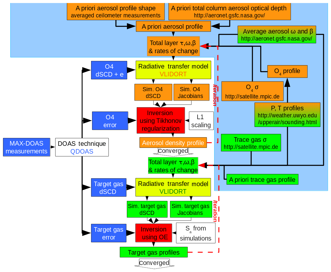
https://www.atmos-meas-tech.net/12/2545/2019/amt-12-2545-2019-f01

Figure 1Flowchart of the complete trace gas retrieval algorithm. Orange boxes belong to the aerosol retrieval and green boxes to trace gas retrieval. The light blue box encompasses forward model input calculation. The dark blue boxes are in- and outputs of QDOAS. The yellow boxes represent the forward modeling steps. The red boxes are the inversion steps, using Tikhonov regularization for aerosol retrieval and optical estimation (OE) for trace gas retrieval.

Download

This remote-sensing technique is based on the spectroscopically resolved measurement of scattered sunlight at different elevation angles, allowing for the retrieval of total column amounts of aerosols and trace gases with profiling capability. Powerful applications of this technique have been demonstrated to provide useful information about the vertical distribution of aerosols (Frieß et al., 2006; Wang et al., 2016) and photochemically relevant species such as nitrogen dioxide (NO₂), formaldehyde (HCHO), glyoxal (CHOCHO) and nitrous acid (HONO) among other gases (e.g., Wittrock et al., 2004; Wagner et al., 2011; Ortega et al., 2015; Hendrick et al., 2014).

Photochemical reactions involving NO₂ play an important role in the formation of O₃ (Finlayson-Pitts and Pitts, 2000). The Mexico City metropolitan area (MCMA) has been particularly affected since the 1990s by high-O₃ episodes threatening the population and forcing the authorities to impose strict restrictions on the usage of motor vehicles (Molina and Molina, 2002). Measurements have been performed in the region using fixed and mobile DOAS zenith-scattered sunlight (Melamed et al., 2009; Johansson et al., 2009; Rivera et al., 2013). In 2014, a MAX-DOAS network, initially consisting of four instruments, was established in the Mexico City metropolitan area (MCMA) and has been operating since (Arellano et al., 2016).

In this contribution, we describe the MMF (Mexican MAX-DOAS Fit) code that has been implemented to retrieve vertical distribution of aerosols and trace gases with emphasis on the errors and diagnostics of the results. An overview of the MAX-DOAS instruments is provided in Sect. 2 and the complete retrieval strategy from the measured spectra to vertical trace gas profiles is summarized in Fig. 1.

Radiative transfer simulations (constituting the forward model in MMF, yellow boxes in Fig. 1) are performed with VLIDORT (Spurr, 2013) to derive simulated differential slant column densities (dSCDs) at the middle of the corresponding wavelength interval used to derive dSCDs from measured spectra. The dSCD retrieval (blue boxes in Fig. 1) is performed with QDOAS (Danckaert et al., 2013) and is described briefly in Sect. 3. The orange parts in the figure refer to the aerosol retrieval while the green parts belong to the trace gas retrieval. Details on the forward model choice, the forward model input calculation (light blue box in Fig. 1) and processing of output quantities in the inversion algorithm are described in Sect. 4.

An error analysis has been included in Sect. 5, in particular investigating the effect of the aerosol retrieval on the NO₂ results. Some examples of the NO₂ variability are provided from one of the network's stations and compared to surface concentrations in Sect. 6, and a summary of the work and an outlook on planned improvements to the retrieval code are presented in Sect. 7.

2 Instruments

An instrument based on the MAX-DOAS technique was designed and developed by the Center for Atmospheric Sciences at the Universidad Nacional Autónoma de México (UNAM). It consists of two main parts: the scanner unit, which collects the scattered light, and the acquisition–control unit, containing a spectrometer and computer that record and store the measurements. The two components are connected by an optical fiber and a data connection cable. Both are described briefly in the following sections. For a more complete description and a map of the area with the station locations and their measurement orientation, we refer the reader to Arellano et al. (2016).

2.1 The scanner

The scanner is composed of a plastic enclosure (NEMA-rated type 3) resistant to sunlight and hermetically sealed to protect the inner parts from water and bugs. This is important in order to assure long measurement periods under harsh conditions (Hönninger et al., 2004; Galle et al., 2010; Arellano et al., 2016). The scattered light is collected by a plano-convex quartz lens (Edmund Optics, ∅=25.4 mm, f=100 mm), focusing it into the entrance of an optical fiber (Fibertech Optica, quartz, 6 m long, ∅=0.6 mm), which transfers the light into the acquisition–control unit. These optical parts are mounted inside a telescope housing constructed of Nylamid material. A shutter system is also installed within the telescope. It consists of a stepper motor (Mercury, 7.5^∘ by step) that rotates a metal circular plate to prevent the passage of light into the optical fiber and an optical switch which is used to indicate the position of the plate. The shutter is used to make measurements of dark spectra in between scans.

A stepper motor (Oriental Motors, PK266-02A) inside the enclosure allows the movement of the scanner unit in a range of 180^∘ with steps of 0.1^∘. A mechanical switch is used as a reference to indicate the starting position of each scan. The motor is controlled by an electronic board composed of an 8-bit microcontroller (AVR architecture), a RS-232 port for communication with the acquisition–control unit, a temperature sensor (Maxim 18B20, accuracy ±0.5 ^∘C) and a dual-axis accelerometer (Analog Devices, accuracy ±0.1^∘) that provides an accurate determination of the telescope's pointing elevation. The theoretical field of view (FOV) of the optical system is 0.31^∘.

2.2 The acquisition–control unit

The second part of the instrument consists of a metallic housing receiving the collected light through the optical fiber and sending it to the spectrometer (Ocean Optics, USB2000+). This commercial device has a crossed asymmetric Czerny–Turner configuration, diffraction grating (1800 lines mm⁻¹) and a slit size of 50 µm wide × 1 mm high, recording spectra in a wavelength range of 289–510 nm at a resolution of 0.69 nm (full width at half maximum). It uses a charge-coupled device (CCD) detector array (Sony ILX511B) of 2048 pixels with an integration time adjustable between 1 ms and 65 s.

Because changes in temperature can affect the wavelength ∕ pixel ratio and also modify the optical properties of the spectrometer like the alignment and the line shape (e.g., Carlson et al., 2010; Coburn et al., 2011), a temperature control system composed of a Peltier cell (Multicomp) and three temperature sensors (Maxim 18B20, accuracy ±0.5 ^∘C) controlled by an electronic board was implemented. The cooling side of the Peltier cell was placed on top of the spectrometer and the heating side was attached to a heat sink. The Peltier cell and the spectrometer were wrapped in a styrofoam box to keep the temperature insulated from the outside. The three temperature sensors were placed on the heat sink, the Peltier cell and the spectrometer to monitor temperature changes. The temperature control system was wrapped in an aluminum enclosure to prevent the heat spreading to other parts of the system and a fan was installed to extract the heat from the enclosure.

The electronic board for the temperature control is composed of an 8-bit microcontroller (AVR, architecture) and a RS-232 communication port. This board is responsible for obtaining the data from the sensors and adjusting the voltage in the Peltier cell to keep the temperature constant.

The acquisition–control unit has a laptop computer (Dell, Latitude 2021) with a Linux operating system contained within the enclosure. The program controlling the hardware is written in C++ using Qt libraries. A script is used to carry out the measurement sequence previously defined and to monitor the spectrometer temperature.

2.3 Measurement strategy

A complete scan consists of a sequence that begins with a measurement towards the zenith (90^∘ elevation angle), followed by tree measurements between elevation angles of 0 and 10^∘ towards the west (for UNAM station, this is an 85^∘ azimuth angle); then 12 measurements are taken with elevation angles between 10^∘ towards the west and 10^∘ towards the east (crossing the zenith, but without taking a measurement), followed by three measurements between 10 and 0^∘ elevation angle towards the east. The same sequence is then repeated but in reverse order. At the end of this cycle, a dark spectrum with the closed shutter is taken. With this setup, a complete scan takes about 7 min. The measurement sequence (90^∘ zenith, 0, 2, 6, 13, 23, 36, 50, 65, 82^∘ W, 82, 65, 50, 36, 23, 13, 6, 2, 0^∘ E) is likely to change in the future to use longer integration times but at the same time reduce the number of viewing directions in the range between a 10^∘ elevation angle towards the west and a 10^∘ elevation angle towards the east in order to keep the total scan time roughly constant.

All data presented in this paper use this setup, meaning that we include both westerly and easterly viewing directions in the same retrieval and hence the result represents an average. This strategy leads to larger fitting errors since this likely deviates further from the assumption of horizontal homogeneity. With our retrieval chain, it is possible to consider the easterly and westerly directions separately to investigate the differences in viewing directions, which is the subject of current investigation.

The output from the MAX-DOAS instruments consists of five files per complete scan: a file containing the metadata of each spectrum (e.g., accelerometer data for each measurement, time of the acquisition, temperatures within the acquisition unit), all the spectra in non-zenith directions, the dark spectrum measured with the shutter closed, a metafile for the dark spectrum and the first zenith reference measurement. These files are stored for further processing.

3 Differential slant column density (dSCD) retrieval

The spectra were evaluated using the QDOAS (version 2.105) software (Danckaert et al., 2013). As a preprocessing step before the QDOAS analysis, the dark signal was subtracted from each of the measurement spectra. A wavelength calibration was conducted in QDOAS by applying a nonlinear least-squares fit to a solar atlas (Kurucz et al., 1984).

For NO₂, the retrieval was conducted in the 405 to 465 nm wavelength range using the spectrum measured at the zenith position at the beginning of each of the measurement sequences as reference. Using a single zenith reference before the scan (both for NO₂ and O₄) instead of a linear interpolation of zenith measurements before and after the scan makes correct measurements during twilight problematic: since upper atmospheric contributions to the slant column density change rapidly during twilight, stratospheric NO₂ could falsely be attributed to the troposphere. Hence, in the study presented here, no twilight measurements are included. For the analysis, differential cross sections of NO₂ at 298 K (Vandaele et al., 1998), O₃ at 221 and 241 K (Burrows et al., 1999), and the oxygen dimer (Hermans et al., 1999) were convolved with the slit function of the spectrometer and a wavelength calibration file (created using a mercury lamp) and using the convolution tool of the QDOAS software. A Ring spectrum, generated at 273 K from a high-resolution Kurucz file using the Ring tool of the QDOAS software (Danckaert et al., 2013), was also included in the analysis.

For O₄, the retrieval was conducted in the 336 to 390 nm wavelength range. Differential cross sections of O₄ (Hermans et al., 1999), O₃ at 221 and 241 K (Burrows et al., 1999), NO₂ at 294 K (Vandaele et al., 1998), BrO at 298 K (Wilmouth et al., 1999), HCHO at 298 K (Meller and Moortgat, 2000), and a Ring spectrum were included in the analysis. A third-degree polynomial was used for the retrievals.

Figure 2 shows the dSCD retrieval error statistics for NO₂ as a function of elevation angle. The plot shows results of 31 448 scans from January to December 2016. Larger dSCD fitting errors are found for viewing angles closer to the horizon (smaller elevation angles), likely due to physical interferences during the measurements. As elevation angles approach the zenith, retrieval dSCD errors decrease considerably. The dSCD errors are the QDOAS calculated errors, a function of the fit residuals and the degree of freedom; see Danckaert et al. (2013) for details.

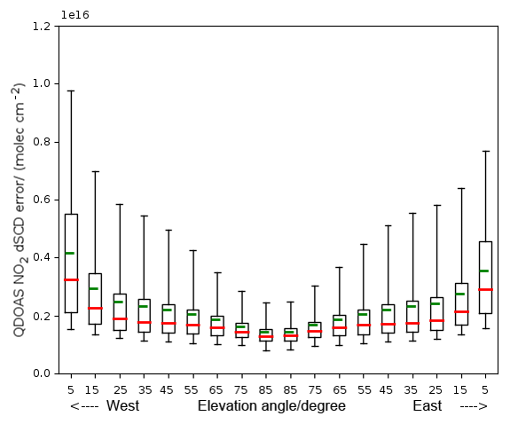
https://www.atmos-meas-tech.net/12/2545/2019/amt-12-2545-2019-f02

Figure 2The dSCD measurement error statistics for NO₂ at the UNAM station as a function of elevation angle for data taken in the year 2016. The box encloses the 25–75th percentiles, the whiskers are 5 %–95 %, and the green bar is the mean and the red bar the median.

Download

4 Mexican MAX-DOAS Fit

The method for the trace gas retrieval from slant column densities using the MMF code is comprised of two parts, an aerosol retrieval using the known O₄ profile, and the trace gas retrieval (e.g., Platt and Stutz, 2008). Both parts consist of the same steps: a forward model and an inversion algorithm.

In Sect. 4.1, details about the inversion strategy are given. Our choice of forward model, VLIDORT (e.g., Spurr et al., 2001; Spurr, 2006, 2013), and the input parameter calculation are detailed in Sect. 4.2. How forward model output quantities are processed for the inversion step is detailed in Sect. 4.3.

The retrieval time per aerosol and trace gas retrieval with the Mexico City setup is roughly half a minute for each scan, but highly dependent on the conditions.

4.1 Inversion theory

The inversion strategy relies on the fact that the problem is sufficiently linear so that in the iteration procedure, the new value for the quantity vector in question x (either the aerosol total extinction per layer or the trace gas optical depth per layer) can be calculated using a Gauss–Newton (GN) scheme¹ according to Eq. (1) (Rodgers, 2000). This step corresponds to the red box and arrows in Fig. 1.

\begin{array}{l} (1) & x_{i + 1} = & x_{a} + {(K_{i}^{T} S_{m}^{- 1} K_{i} + R)}^{- 1} K_{i}^{T} S_{m} \\ [(y - F (x_{i})) - K_{i} (x_{a} - x_{i})] \end{array}

Here, superscript “T” denotes transposed; superscript “−1” denotes the inverse. The index i is the iteration index; the subscript “a” indicates a priori values. S_m is the measurement error covariance matrix, and y denotes the vector of measured differential slant column densities. F(x_i) are the simulated differential slant column densities, calculated using the forward model with input profile x_i. Both y and F(x_i) are vectors of dimension, which is the number of telescope viewing angles. $K_{i} = \partial F (x)^{l} / \partial x_{n}$ is the Jacobian matrix at the ith iteration describing the change in simulated dSCD for viewing angle l when the profile x in layer n is varied.

In the case of optimal estimation (OE), the regularization matrix R is equal to the inverse of the a priori covariance matrix, $R = S_{a}^{- 1}$ . OE regularization is used for trace gas retrieval. Other regularization matrices are possible; see, e.g., Steck (2002).

For the aerosol retrieval used in this study, we use the L1 operator (R=L1^TαL1) where the scaling parameter α is set to a constant value of 20 and is supplied via an input script to limit the degrees of freedom (DOFs) to just slightly above 1. Different scalings for the upper layers and lower layers could be supplied, as well as a complete regularization matrix R.

4.2 Forward model

Several radiative transfer codes have been developed to serve as forward models for this kind of retrieval algorithms. For example, there are Monte Carlo (MC) codes, such as AMFTRAN (Marquard, 1998), TRACY (von Friedeburg et al., 2002; von Friedeburg, 2003) or PROMSAR (Palazzi et al., 2005). All these MC radiative transfer codes start with ejecting photons from the instrument and following the photon path backwards (see also, e.g., Perliski and Solomon, 1993; Marquard et al., 2000); hence they are sometimes somewhat confusingly referred to as backward models. The advantage of MC codes is their high accuracy; the disadvantage is the rather long calculation time. SCIATRAN (e.g., Buchwitz et al., 1998; Rozanov et al., 2014, 2017) combines multiple-scattering radiative transfer modeling using the Picard iterative approximation and a chemistry and an inversion code. It has been heavily used in NO₂ (e.g., Vidot et al., 2010) and ozone (e.g., Rahpoe et al., 2013 b, a) retrieval from satellite observations.

Another class of radiative transfer codes, such as VLIDORT and DISORT (Stamnes et al., 1988; Dahlback and Stamnes, 1991), uses the discrete ordinate algorithm. This finite difference method is based on finding solutions for an atmosphere consisting of a number of homogeneous layers using Gaussian quadrature approximations to the integrodifferential radiative transfer equation expressed using Legendre polynomials for the phase function and Fourier series for the intensity.

The big advantage of the second class of codes is their high speed. Another advantage of VLIDORT is that it calculates not only the intensity but also analytic Jacobians. The number of calls to the program is not equal to twice the number of layers (as it would need to be for finite difference approximation), but a single call is sufficient. MMF uses the intensity part of VLIDORT, version 2.7, released in August 2014. (V)LIDORT is configured to return intensity Jacobians with respect to gas absorption layer properties or aerosol total extinction layer properties.

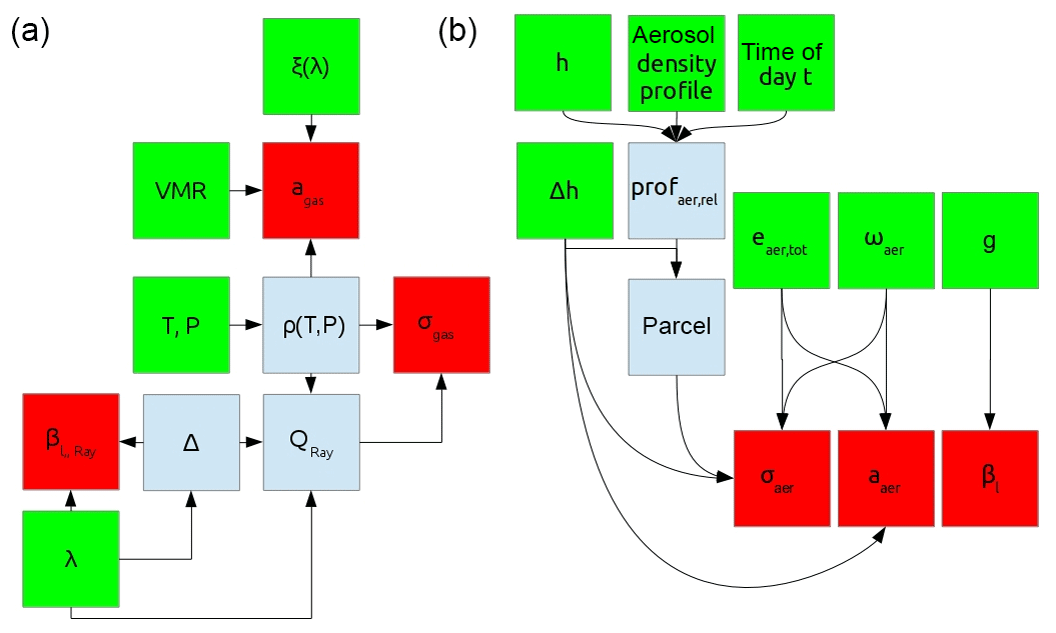
https://www.atmos-meas-tech.net/12/2545/2019/amt-12-2545-2019-f03

Figure 3Calculating the gas and air (a) and aerosol (b) contributions to the layer input parameters for VLIDORT. The green boxes are primary input to MMF, blue boxes are intermediate quantities and red boxes are final outputs that are combined for VLIDORT layer input. Here VMR denotes the a priori volume mixing ratio. Instead of a VMR, an a priori trace gas density can be supplied, too.

Download

In MMF, the simulation grid is supplied via an input file to the code together with the corresponding a priori values of the trace gas concentration and the aerosol profile. The retrieval can be performed on the whole simulation grid or only on the lower part of the simulation grid. In this study, the simulation grid is identical to the retrieval grid and the layer distribution of the retrieval grid is not equidistant. The grid consists of 22 layers up to 25 km. The layer thickness increases from 100 m at the lowest layer to 5 km in the uppermost layer. The exact height distribution can be seen in Fig. 5. The surface albedo used in this study was set to 0.07; this value can be passed to MMF in the configuration file. However, in practice the effect for downwelling intensity and hence for the dSCD calculation was found to be negligible.

For each simulated atmospheric layer, the following input needs to be supplied to VLIDORT²:

total layer optical depth, τ;
single-scattering albedo, ω;
phase function expansion coefficients, β.

Since Jacobians with respect to changes of quantity χ in each layer are required, the normalized derivatives of the total primary optical quantities, τ, ω and β, with respect to this quantity need to be supplied as well. In the case of trace gas retrieval, χ=a_gasΔh, and in the case of aerosol retrieval, $χ = (σ_{aer} + a_{aer}) Δ h$ . Here, a_gas and a_aer are the gaseous and aerosol absorption coefficients, respectively, and σ_aer is the aerosol scattering coefficient. Δh is the layer thickness. Hence, for each layer the following input is additionally required:

4.
normalized rate of change in τ with respect to χ,
5.
normalized rate of change in ω with respect to χ,
6.
normalized rate of change in β with respect to χ.

In order to calculate this input, we first need to calculate the separate properties for the trace gases and the aerosols. Afterwards, these quantities are combined to yield the total layer quantities.

The calculation of the contribution from the trace gas and the air density (through Rayleigh scattering) for the layer inputs (one to six) is presented in Sect. 4.2.1. The aerosol contribution calculation is outlined in Sect. 4.2.2. These two sections also contain information on the source of information for the respective a priori values, as well as, for gas, the error covariance matrix.

The calculation of the contributions from gas and aerosol to yield the VLIDORT inputs (one to six) is detailed in Sect. 4.2.3.

4.2.1 Input for gases

In Fig. 3a, the steps to calculate the contribution of the trace gas and the contribution from Rayleigh scattering in each layer are outlined. Red boxes represent the trace gas (and air) contribution to VLIDORT input quantities, green boxes are primary inputs to the inversion code and light blue boxes are intermediate quantities that are neither direct input to MMF nor final input for the forward model.

The a priori volume mixing ratio (VMR) profile and the covariance matrix for this study are calculated from simulations covering the year 2011 using WRF-Chem v3.6. The model domain covers Mexico and surrounding seas; the domain has 200-by-100 square grid cells with approximately 28 km width and 35 vertical layers. The following WRF parameterizations were used: WRF single-moment three-class scheme (mp_physics = 3), planetary boundary layer (PBL, bl_pbl_physics = 1), and cumulus option Grell 3-D ensemble scheme (cu_physics = 5). As a land-surface option, the unified Noah land use surface model (sf_surface_physics = 2) was used. The time-varying sea surface temperature parameter was set to “on”, the grid analysis nudging parameter was set to “on” and the urban canopy model was set to “off”. The emissions used were for the RADM2 mechanism and are from the National Emissions Inventory 2008.

MMF takes pressure and temperature profiles on a separate height grid; internal interpolation to the provided retrieval grid is performed. In the processing chain implemented in Mexico, the temperature and pressure profiles from radiosonde data for the specific day are downloaded from the University of Wyoming (http://weather.uwyo.edu/upperair/sounding.html, last access: 9 April 2019) from the Mexico City International Airport, station number 76679. These temperature and pressure profiles are linearly interpolated to the simulation grid used to calculate the dry air number density ρ; see Appendix B.

The absorption cross section ξ_λ is taken at a wavelength in the middle of the wavelength interval used for the QDOAS retrieval (see Sect. 3): for aerosol retrieval it is 361 nm and for NO₂ it is 414 nm. The same cross-section tables as for QDOAS dSCD retrievals (see Sect. 3) are used for NO₂ and O₄. However, since the cross section cancels out at the end of the calculation, its exact value is not too important.

There are analytical fits to the temperature dependence, using linear (e.g. Vandaele et al., 2003, for NO₂) or more complicated (e.g. Kirmse et al., 1997) temperature dependences, for example. For a comparison study of different fitting functions, see Orphal (2002). These could be implemented; however, the cross section is currently not temperature dependent, in agreement with the assumption made for defining dSCDs.

The trace gas absorption coefficient is calculated according to Eq. (2):

\begin{matrix} (2) & a_{gas} = VMR \cdot ξ_{λ} \cdot ρ . \end{matrix}

For the calculation of the depolarization ratio Δ, the main contributions are from N₂, CO₂, O₂ and Ar. Our implementation follows Bates (1984). Details are given in Appendix B. For the calculation of the Rayleigh cross section Q_Ray, we follow the implementation of Goody and Yung (1989) (their Eq. 7.37); see also Platt et al. (2007) (their Eq. 19.5). The air scattering coefficient can then be calculated according to Eq. (3):

\begin{matrix} (3) & σ_{air} = Q_{Ray} \cdot ρ, \end{matrix}

and the Rayleigh scattering expansion coefficients β_l (e.g., Spurr et al., 2001) can be calculated according to Eq. (4):

\begin{matrix} (4) & β_{air 0} = 1, β_{air, 1} = 0, β_{air, 2} = (1 - Δ) / (2 + Δ) . \end{matrix}

4.2.2 Input for aerosols

The (a priori) aerosol data for total optical depth, average single-scattering albedo ω and asymmetry parameter g (used to calculate the phase function moments) are time interpolated values from the co-located AERONET (Aerosol Robotic Network) station in Mexico City (V2, level 1.5 at http://aeronet.gsfc.nasa.gov, last access: 5 November 2018). They are also extra- and interpolated at the retrieval wavelength. The a priori shape of the profile is taken from hourly averaged ceilometer data (García-Franco et al., 2018), interpolated at the middle layer height h of each layer.

The first part of MMF, the aerosol retrieval, is limited to the aerosol density profile and the total aerosol optical depth. The average single-scattering albedo ω and asymmetry parameter g are not subject to retrieval and are assumed to be constant in all layers.

Figure 3b outlines the strategy how the aerosol contribution to the VLIDORT layer input parameters is calculated.

The hourly averages of (relative) aerosol density profiles in arbitrary units from ceilometer measurements between November 2009 and February 2013 are interpolated at measurement day time t and at retrieval grid middle heights h to provide a relative aerosol profile. This profile, turned into a partial optical depth per layer by multiplying with the layer thickness, is scaled to match the total aerosol extinction from AERONET τ_aer. The profile is then converted back into an intensive³ quantity by division by layer thickness, usually known as the aerosol extinction profile (extinction per unit length, AE). This is then used to calculate the aerosol scattering coefficient σ_aer in each layer by multiplying the layer aerosol extinction with the aerosol single-scattering albedo ω_aer.

The aerosol absorption coefficient a_aer is the layer aerosol extinction times (1−ω_aer), and the aerosol phase function coefficients β_aer,l can be calculated via the Henyey–Greenstein phase function and the asymmetry parameter g (see Eq. 5) e.g., Hess et al. (1998), where l denotes the moment,

\begin{matrix} (5) & β_{aer, l} = (2 l + 1) \cdot g^{l} . \end{matrix}

4.2.3 Calculating final VLIDORT input

As mentioned in the introduction to this section, the layer input parameters for VLIDORT are total optical depth τ and single-scattering albedo ω in the layer, as well as the phase function coefficients β_l. The quantities which have been calculated so far are the aerosol and air contributions to β_l and the air and aerosol scattering coefficients σ_air and σ_aer, as well as the absorption coefficients a_gas from the trace gas in question and a_aer from the aerosol in each VLIDORT input layer (red boxes in Fig. 3). These quantities need to be combined to total layer input parameters.

The total layer optical depth is simply the product of the layer thickness and the sum of all extinction and scattering coefficients; see Eq. (6):

\begin{matrix} (6) & τ = Δ h \cdot (σ_{air} + σ_{aer} + a_{gas} + a_{aer}) . \end{matrix}

The combined single-scattering albedo can be calculated as in Eq. (7):

\begin{matrix} (7) & ω = (σ_{air} + σ_{aer}) \cdot Δ h / τ . \end{matrix}

The combined expansion coefficients are calculated as in Eq. (8):

\begin{matrix} (8) & β_{l} = (β_{air, l} \cdot σ_{air} + β_{aer, l} \cdot σ_{aer}) / (σ_{air} + σ_{aer}) . \end{matrix}

Since Jacobians with respect to changes in quantity χ in each layer are required, the normalized derivatives of the total primary optical quantities, τ, ω and β, with respect to this quantity need to be supplied. In the case of trace gas retrieval, χ=a_gasΔh, and in the case of aerosol retrieval, $χ = σ_{aer} Δ h + a_{aer} Δ h$ . Therefore, what needs to be done is to calculate the normalized derivatives of Eqs. (6)–(8) with respect to these quantities. It should be remembered that β is a vector.

The three quantities for aerosol are calculated according to Eqs. (9)–(11).

\begin{array}{l} (9) & \frac{χ}{τ} \frac{d τ}{d χ} = & \frac{(σ_{aer} + a_{aer}) Δ h}{τ} \frac{d τ}{d (σ_{aer} + a_{aer}) Δ h} \\ = & \frac{σ_{aer} + a_{aer}}{e} \\ (10) & \frac{χ}{ω} \frac{d ω}{d χ} = & \frac{(σ_{aer} + a_{aer}) Δ h}{ω} \cdot [\frac{\partial ω}{\partial σ_{aer}} \\ \frac{d σ_{aer}}{d [(σ_{aer} + a_{aer}) Δ h]} + \frac{\partial ω}{\partial a_{aer}} \frac{d a_{aer}}{d [(σ_{aer} + a_{aer}) Δ h]}] \\ = \frac{σ_{aer} a_{gas} - a_{aer} σ_{air}}{ω e^{2}} \\ (11) & \frac{χ}{β} \frac{d β}{d χ} = & \frac{(σ_{aer} + a_{aer}) Δ h}{β} \frac{d β}{d (σ_{aer} + a_{aer}) Δ h} \\ = & \frac{σ_{aer}}{β} \frac{β_{aer} - β}{σ_{aer} + σ_{air}} \end{array}

Here, e is the total extinction coefficient: $e = τ / Δ h$

For the trace gas Jacobian calculation, the corresponding normalized derivatives are according to Eqs. (12)–(14).

\begin{array}{l} (12) & \frac{χ}{τ} \frac{d τ}{d χ} = \frac{a_{gas} Δ h}{τ} \frac{d τ}{d a_{gas}} = \frac{a_{gas}}{e} \\ (13) & \frac{χ}{ω} \frac{d ω}{d χ} = \frac{a_{gas} Δ h}{ω} \frac{ω}{a_{gas}} = - \frac{a_{gas}}{e} \\ (14) & \frac{χ}{β} \frac{d β}{d χ} = 0 \end{array}

4.3 Calculating dSCDs and weighting functions

The forward model outputs, intensities and intensity Jacobians need to be converted into differential slant column densities and corresponding Jacobians. For each set of dSCDs, we have to run the forward model two times: Once with the gas absorption included and once without the gas absorption. Each of these sets consists of simulations in the desired telescope directions and one simulation towards the zenith. Note that the output from VLIDORT is Kx; hence the immediate output from VLIDORT has to be divided by x in case of linear retrieval to give the Jacobian alone.

In the following, the intensity and Jacobian of the simulation towards the desired angles without gas absorption are denoted $I_{0}^{α}$ and $K_{0}^{α}$ , the intensity (Jacobian) with gas absorption towards the zenith $I_{g}^{z}$ ( $K_{g}^{z}$ ), the intensity (Jacobian) with gas absorption towards the desired angle $I_{g}^{α}$ ( $K_{g}^{α}$ ) and the intensity (Jacobian) without gas absorption towards the zenith $I_{0}^{z}$ ( $K_{0}^{z}$ ). The dSCD can be calculated as in Eq. (15).

\begin{matrix} (15) & {dSCD}^{α} = \ln (\frac{I_{0}^{α} \cdot I_{g}^{z}}{I_{g}^{α} \cdot I_{0}^{z}}) / ξ_{λ} \end{matrix}

The corresponding weighting function K is calculated as in Eq.16:

\begin{matrix} (16) & K^{α} = \frac{(K_{0}^{α} I_{g}^{z} I_{g}^{α} I_{0}^{z} + I_{0}^{α} K_{g}^{z} I_{g}^{α} I_{0}^{z} - I_{0}^{α} I_{g}^{z} K_{g}^{α} I_{0}^{z} - I_{0}^{α} I_{g}^{z} I_{g}^{α} K_{0}^{α})}{(I_{0}^{α} I_{g}^{z} I_{g}^{α} I_{0}^{z} ξ_{λ})} . \end{matrix}

5 Error analysis

The errors of gas profile retrievals in remote-sensing applications can be divided into the following four different types (Rodgers, 2000):

smoothing error, arising from the constraint of the NO₂ and aerosol profiles;
measurement noise error, arising from the noise in the spectra;
parameter error, including different parameters as aerosol profiles and cross sections; and the
forward model error, which originates from the simplification and uncertainties in the radiative transfer algorithm.

The gain matrix, as defined by Eq. (17), describes the change in retrieved x when measurement y changes. It can hence be used to map the uncertainty in measurement space to a state-vector uncertainty.

\begin{matrix} (17) & gain := \frac{\partial x}{\partial y} = {(K_{i}^{T} S_{m}^{- 1} K_{i} + R)}^{- 1} K_{i}^{T} S_{m} \end{matrix}

The error analysis in general produces an error pattern ϵ_y in the measurement space of vectors of the dSCDs retrieved by QDOAS and simulated by MMF. With help of the gain matrix, this error pattern is then mapped as ϵ_x into the space of the solution state.

5.1 Smoothing error

The retrieved atmospheric state vector x only represents a smoothed version of the true real state. The partial column averaging kernel matrix AK_pcol describes how a change in the true atmospheric state vector x_true is translated into changes in the retrieved state vector x, according to Eq. (18):

\begin{matrix} (18) & x - x_{a} = {AK}_{pcol} (x_{true} - x_{a}) + ϵ_{x} . \end{matrix}

The averaging kernel of the partial column and total column (AK_tot) describe how the retrieved solution profile depends on the real atmosphere x_true. They have to be taken into account if the profile and the column are used. The part which is not explained by AK_pcol is explained by the retrieval error ϵ_x.

As MMF uses constrained least-square fitting, the AK_pcol is calculated analytically by MMF itself for each scan according to Eq. (19):

\begin{matrix} (19) & {AK}_{pcol} := \underset{definition}{\underset{︸}{\frac{\partial x}{\partial x_{true}}}} = \underset{analytical calculation}{\underset{︸}{gain \cdot K}} . \end{matrix}

The averaging kernel matrix is in general asymmetrical. The columns represent response functions related to a perturbation in a certain layer. The rows of the matrix represent the sensitivity of the NO₂ partial column of a certain layer (or concentration in a certain layer) to all the different true partial columns or concentrations.

If AK_pcol is expressed in units of partial columns (as here indicated by the subscript “pcol”), the sum of the rows is the total column averaging kernel. It represents the sensitivity of the vertical column density (VCD) to the anomalies in different heights.

The change in averaging kernel under transformation of the units is expressed by two matrix multiplications: one by multiplying the diagonal matrix containing the partial air column in its diagonal U_aircols from the right with the averaging kernel and the other by multiplying the inverse of the diagonal matrix $U_{aircols}^{- 1}$ from the left side with the averaging kernel; see Eq. (20):

\begin{matrix} (20) & {AK}_{VMR} = U_{aircols}^{- 1} \cdot {AK}_{pcol} \cdot U_{aircols} . \end{matrix}

The trace of the AK_tot matrix represents the DOF, the number of independent pieces of information in the profile retrieval, which is around two for the NO₂ retrieval.

Equation (18) separates the smoothing effect described with AK matrices from the other errors. Before comparing the retrieved profiles of MMF with profiles from models or other measurements, such as satellite measurements, it is necessary to smooth the profile from the other source with the AK from MMF (Rodgers and Connor, 2003). Alternatively, a smoothing error S_smooth for the profile can be calculated according to Rodgers (2000) from the a priori covariance matrix S_a and the averaging kernel. The latter is describing how the true atmospheric state varies, as a best estimate. Equation (21) describes how sensitivity of the retrieved atmospheric state vector depends on the true atmospheric state:

\begin{matrix} (21) & AK = \frac{\partial x}{\partial x_{true}} . \end{matrix}

Both quantities can be given in different representations adjusted to the atmospheric state vector as a fraction of the a priori, the VMR (“VMR”), as number densities or as partial column profiles (“pcol”) as used above. Using AK_VMR, S_smooth can be calculated according to Eq. (22):

\begin{matrix} (22) & S_{smooth} = ({AK}_{VMR} - 1) S_{a}, VMR ({AK}_{VMR} - 1)^{T} . \end{matrix}

The smoothing error for the VCD is then calculated from the full covariance matrix of the smoothing error S_smooth using a total column operator; see Eq. (23):

\begin{matrix} (23) & σ_{smooth} = \sqrt{g^{T} \cdot \underset{︸}{({AK}_{pcol} - 1) S_{a,pcol} ({AK}_{pcol} - 1)^{T} S_{smooth}^{pcol} \cdot g}}, \end{matrix}

where g is the total column operator for partial column profiles: $g^{T} = (1, 1, 1, 1, 1, 1, 1, 1, 1, \dots 1)$ .

As described before, the NO₂ retrieval code uses a single a priori profile and covariance matrix taken from the chemical transport model WRF-Chem. This results in the sensitivities and smoothing errors represented in Fig. 4a.

The aerosol retrieval, however, uses a Tikhonov constraint and no covariance matrix is available. The a priori values for the aerosol extinction profile are reconstructed by the actual total aerosol optical depth reported by the daily AERONET measurements and the average vertical distribution, reconstructed from ceilometer measurements for each hour of the day. The covariance matrix for the aerosols S_{a, aerosol} is obtained by assuming a 100 % variability of the used a priori profile and an exponential correlation length of η=500 m between the different layers, as in the recent work by Wang et al. (2017); see Eq. (24):

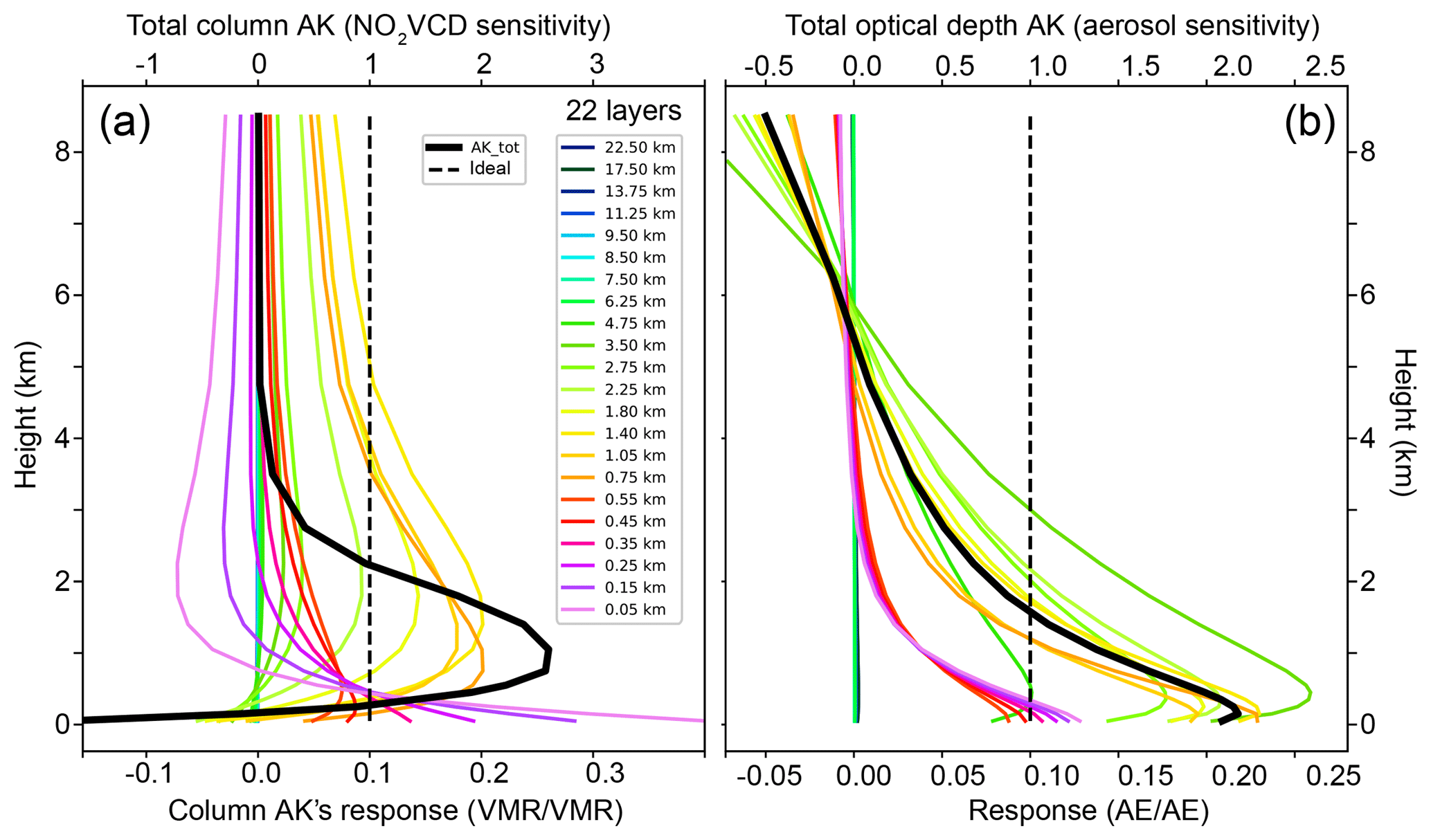
\begin{matrix} (24) & S_{a, aerosol} [i, j] = (100 % \cdot A E_{a} [i] \cdot A E_{a} [j]) \exp^{(- | z [i] - z [j] | / η)} . \end{matrix}

https://www.atmos-meas-tech.net/12/2545/2019/amt-12-2545-2019-f04

Figure 4Averaging kernel columns: (a) in VMR representation for NO₂ profile retrieval and (b) in the corresponding intensive quantity for the aerosol extinction (AE) profile. Each colored line shows the expected response on perturbation in a certain layer and belongs to the lower axis. The total column averaging kernel, (a) for the NO₂ VCD and (b) for the total optical depth, is given as a black line and belongs to the upper axis. The vertical dashed line in each panel indicates an ideal sensitivity of 1.0 at all altitudes.

Download

In the cases where no vertical aerosol extinction profile (AE profile) retrieval is available because the retrieval failed, or no O₄ dSCDs were available in the first place, a NO₂ profile can still be retrieved by using the a priori AE profile instead of the retrieved one. Since in that case no information of the O₄ absorption is used, the estimated smoothing error S_smooth is then directly given by the a priori covariance matrix S_a,aerosol for the AE profile. The a priori information about the optical properties described by the aerosol extinction profile is designed for cloud-free days and therefore the error analysis is just valid for such cloud-free days.

We have assumed a constant sensitivity AK and a constant a priori covariance matrix S_a for the calculation. The AK of the trace gas profile indeed depends strongly on the aerosol profile. It also depends slightly on the trace gas profile itself. The S_a covariance matrix of the aerosol extinction profile should be given for each hour as the a priori profile varies with time of day. Therefore, the estimation of the smoothing error as it is calculated here gives just a rough general idea about the size of the smoothing error.

5.2 Measurement noise

The measurement noise error can be calculated from the gain matrix and the measurement noise matrix (S_m) (Rodgers, 2000). The diagonal matrix (S_m) is already used in the optimal estimation of the profile retrieval to weight the different dSCDs of a scan according to the square of the errors from the QDOAS retrievals. The statistics of the measurement dSCD errors and its dependence on the elevation angle have been presented in Fig. 2.

The measurement noise error matrix for both (1) the NO₂ profile and (2) aerosol extinction profile are calculated directly during the retrieval and are available from the MMF output of each measurement sequence as a full covariance matrix S_noise, given in units of partial columns and partial optical depths. The NO₂ total column error is then calculated from this and the total column operator, and amounts to around 2.4 % of the VCD (see line 2 in Table 1). The errors in the profile are shown in Fig. 6.

Table 1Errors in NO₂ vertical column density as a fraction of a retrieved VCD of 3.2×10¹⁶ molec. cm⁻² measured at 13:58 on 20 May 2016 (UTC − 6). The total error is calculated as the square root of the sum of squares of different independent errors. Different total errors are calculated, by including or not including the algorithm error (Wang et al., 2017), considering the two cases: that an aerosol extinction profile is retrieved from O₄ absorption or just an a priori guess is used. For the assumed variability of the aerosol extinction, the error due to the uncertainty remaining after an aerosol extinction profile retrieval is 5.1 % instead of 9.8 %. However, if the algorithm error according to Wang et al. (2017) is included, the remaining error due to the uncertainty in the aerosol profile is slightly better: 9.3 % instead of the 9.8 % without O₄ retrieval.

Download Print Version | Download XLSX

5.3 Parameter errors

The parameter errors originate from all uncertainties in input parameters in the forward model that are not properly fitted. These are, for example, the cross sections and, for the NO₂ profile retrieval, also the used aerosol extinction profile.

5.3.1 Parameter error from spectroscopy

The error originating from an uncertainty in the cross section of 3 % (Wang et al., 2017) is also around 3.0 % in the vertical column (see line 3 in Table 1) and similar in the vertical profile. This error can be calculated using the generalized measurement error covariance matrix $S_{spectroscopic}^{y}$ in the measurement space assuming that all retrieved dSCDs are 3 % too high (or low) and using the outer product of the measurement state vector containing the retrieved dSCDs; see Eq. (25):

\begin{matrix} (25) & S_{spectroscopic}^{y} = (3.0 %)^{2} \cdot y y^{T} . \end{matrix}

Using the gain matrix (see Eq. 17), this can be translated into an error in the retrieval space, as demonstrated in Eq. (26):

\begin{matrix} (26) & S_{spectroscopic}^{x} = gain \cdot S_{spectroscopic}^{y} \cdot {gain}^{T} . \end{matrix}

From the $S_{spectroscopic}^{x}$ matrix, the error in the total column and profile is calculated as shown earlier in Sect. 5.1. As expected, the error for the total column is 3 % and the errors in the NO₂ VMR profile are shown in Fig. 6. The spectroscopic error is a purely systematic error and affects all retrievals in the same manner.

5.3.2 Parameter error from aerosol profile

The AE profile is crucial for the NO₂ profile retrieval because of its strong contribution to the air mass factor. The uncertainties in this vector of input parameters arise from errors in the aerosol extinction profile retrieved from the spectral signature of the O₄ dimer. For the propagation of the error of the O₄ AE retrieval into the NO₂ retrieval, we assume here that the total error in the AE profile depends on just the two contributions: (a) smoothing error and (b) measurement noise errors.

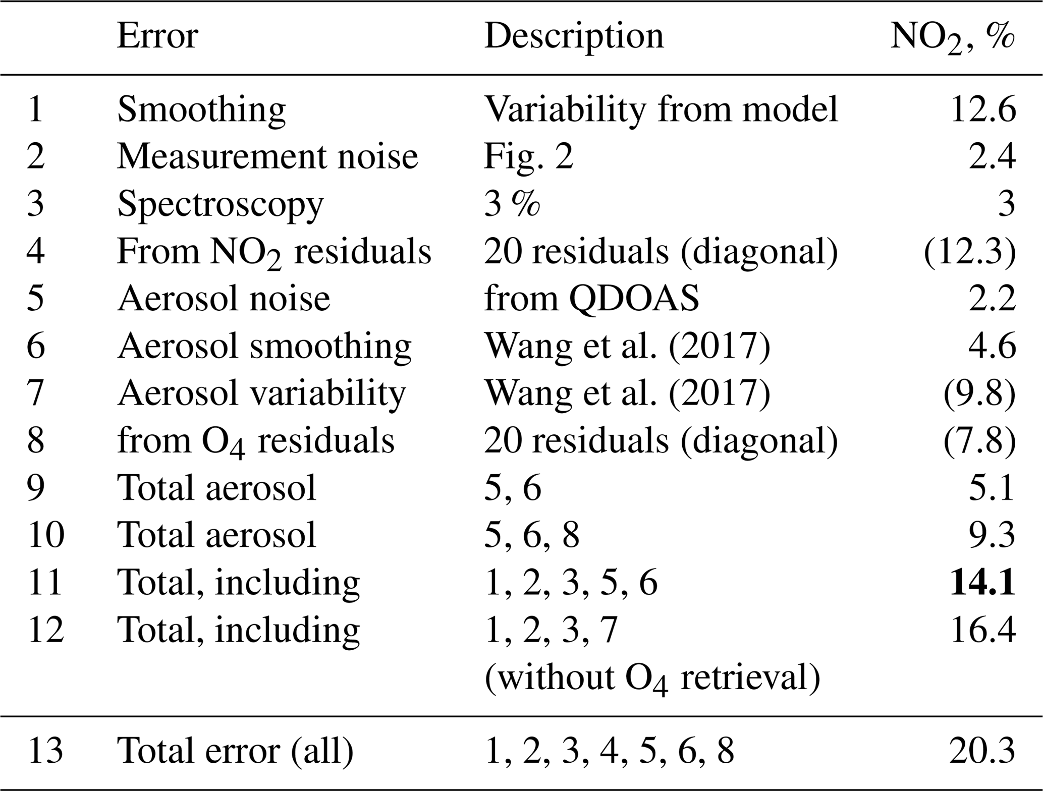
The effect of the assumed aerosol content in each layer on the retrieved NO₂ profile is calculated by a sensitivity study. For this, 22 NO₂ retrievals are performed for the same measurement sequence (dSCDs) using slightly modified aerosol extinction profiles. First, a normal retrieval with the best estimated aerosol extinction profile is retrieved. Then, the aerosol extinction profile is modified so that the partial extinction of the ith layer is increased by 1 % of the total optical depth with respect to the original aerosol extinction profile.

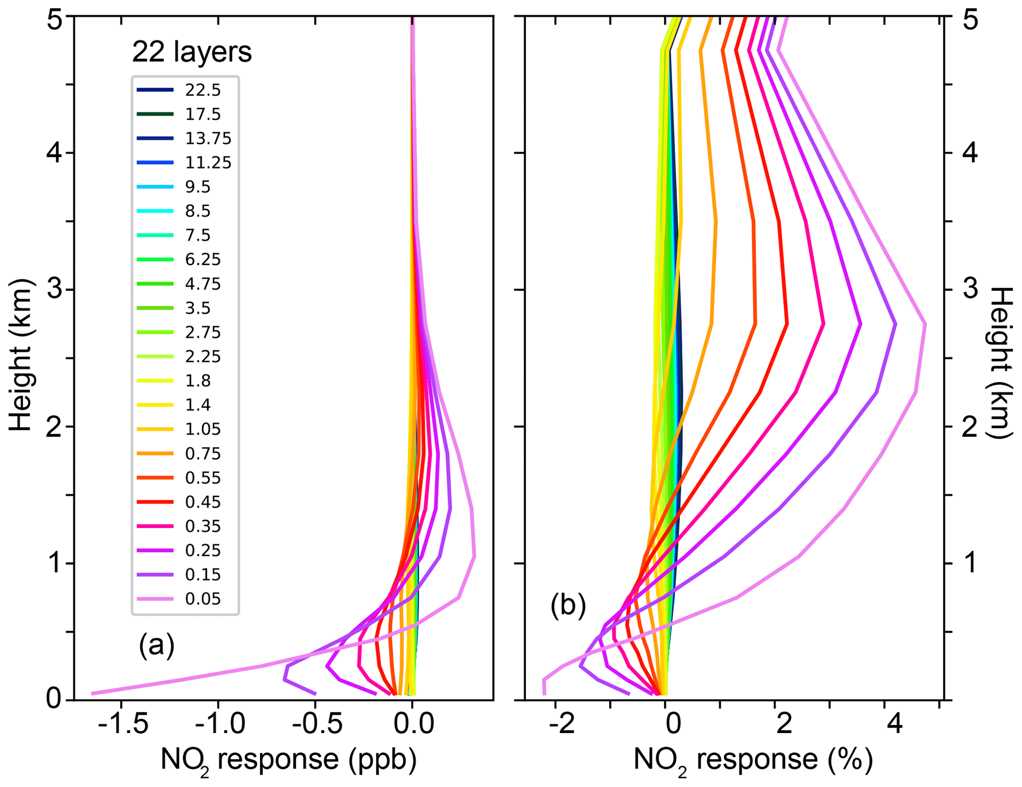
https://www.atmos-meas-tech.net/12/2545/2019/amt-12-2545-2019-f05

Figure 5Plots showing the results of how sensitive the NO₂ profile is to changes in the aerosol extinction profile. (a) Columns of the matrix D created to describe the response in the NO₂ VMR profile (the differences with respect to the original retrieval). (b) Same as (a) but the response to the perturbation in the aerosol profile is given as a fraction of the retrieved NO₂ profile.

Download

The difference between the perturbed and original NO₂ VMR profiles is combined into the matrix D, thus describing how the NO₂ VMR profile responds to changes in the aerosol at different heights. The result is presented in Fig. 5.

With the help of this matrix, D_VMR, the different errors in the aerosol extinction profile, as measurement noise (see Sect. 5.2), smoothing error (see Sect. 5.1) or even due to the algorithm error according to Wang et al. (2017), can be propagated to the NO₂ profile and its VCD. The uncertainty in aerosol, represented by its S_{a, aerosol} matrix (see Eq. 24), translates into an uncertainty in NO₂ VMR according to Eq. (27):

\begin{matrix} (27) & S_{{NO}_{2} - VMR}^{aerosol} = D_{VMR} S_{a,aerosol} D_{VMR}^{T} . \end{matrix}

Using the technique from Eq. (23) with the unit transformation for the AK as in Eq. (20), this translates into an error on the VCD as in Eq. (28).

\begin{array}{l} (28) & {Error}_{{NO}_{2} - VCD}^{aerosol} = \\ \sqrt{g^{T} U_{aircols} \cdot D_{VMR} \cdot S_{a,aerosol} \cdot {D_{VMR}}^{T} U_{aircols} \cdot g} \end{array}

The propagation of the smoothing and measurement noise errors of the O₄ retrieval into the NO₂ retrieval (separately resulting in 4.6 % and 2.2 %; see lines 6 and 5 in Table 1, respectively) results in a 5.1 % error in the NO₂ VCD (see line 9 in Table 1). If the algorithm error introduced by Wang et al. (2017) (7.8 %, line 8 in Table 1) is included in the error propagated to NO₂, the error in NO₂ VCD is 9.3 % (line 10 in Table 1). However the algorithm error is calculated from the resulting residual of the fit and is dependent on the other error sources as mentioned earlier.

If no O₄ retrieval is performed successfully, the aerosol a priori profile is used for the NO₂ retrieval. The error in this aerosol profile is estimated by its aforementioned assumed variability and S_a covariance matrix: a variability of 100 % of the a priori profile is assumed for calculating the diagonal elements and an exponential correlation length of 500 m is used for calculating the off-axis elements of the S_a matrix. The error in the NO₂ VCD would in this case be 9.8 % (see line 7 in Table 1).

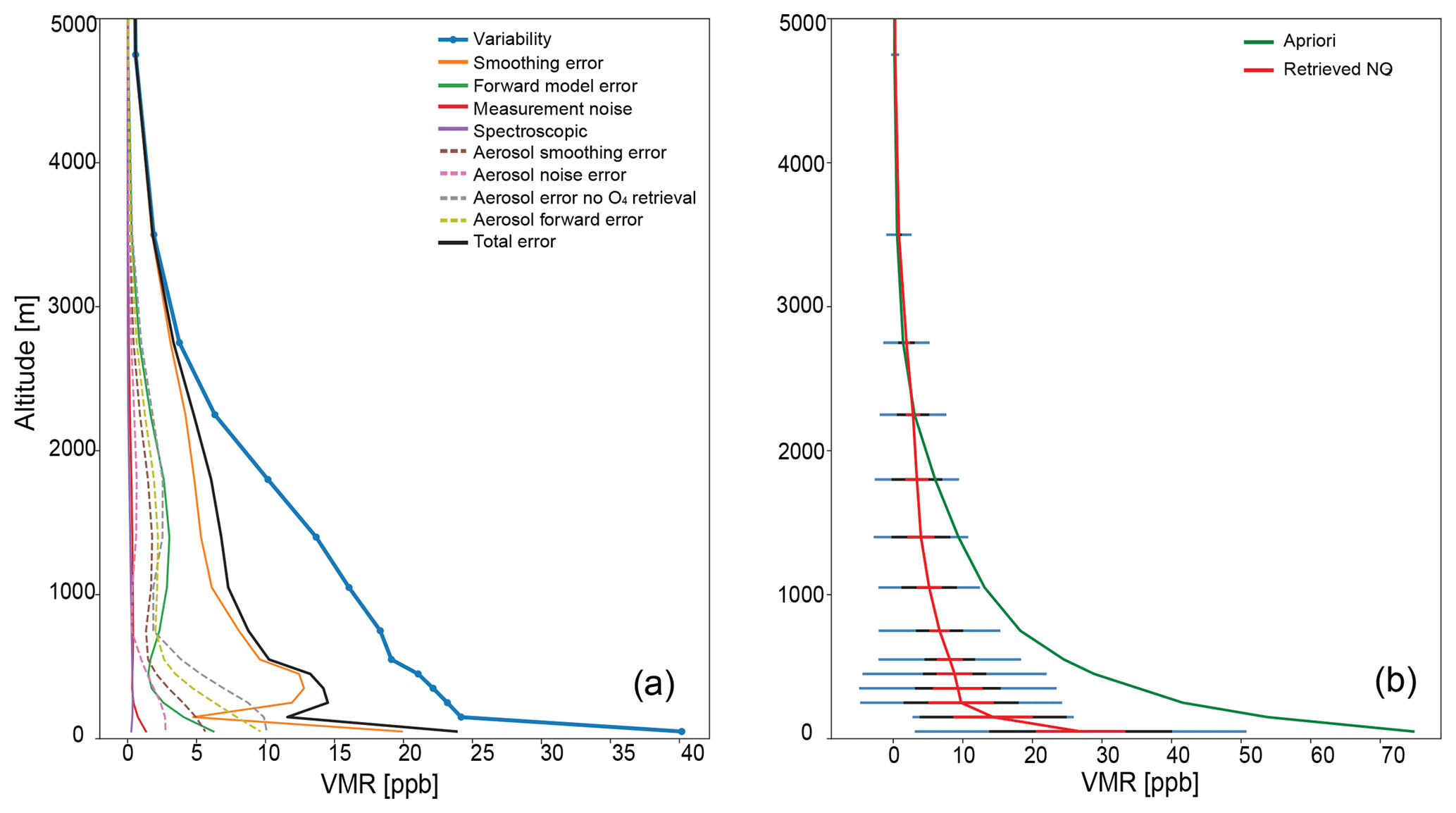
https://www.atmos-meas-tech.net/12/2545/2019/amt-12-2545-2019-f06

Figure 6Altitude-dependent errors in a NO₂ VMR profile measured at 13:58 on 20 May 2016 (UTC − 6). (a) The square root of the diagonal in the covariance matrix describing the individual error contributions in the VMR profile and (b) the retrieved NO₂ VMR profile with corresponding error bars (total error and variability). Panel (a) also includes the a priori profile in green.

Download

5.4 Forward model error

The forward model error could be evaluated if an improved forward model was available. However, this is not the case. Errors in the forward model would result in systematic structures in the residual and a larger residual than expected from the error calculated by QDOAS for the slant columns. The least supported simplification in the forward model is the assumption of a horizontal homogeneity of gas and aerosols. A horizontal inhomogeneity leads to a set of slant columns in a scan which cannot be simulated by VLIDORT and the residuals of measured minus calculated slant columns indicate this error. Following Wang et al. (2017), we calculate the variance in the residuals as a function of viewing angle and hence the algorithm error. But as all errors increase the residual the so-called algorithm error is not identical to the forward model error. However, it is maybe a good way to check empirically if there are important error contributions missing in the analytical analysis.

5.5 Total error

The results from the error estimations are summarized in Table 1. The overall error in the NO₂ VCD is estimated to be around 14.1 % (20.3 % including the algorithm errors for NO₂ and O₄ calculated from the residuals). The contributions are 12.5 % from smoothing, 2.4 % from measurement noise, 3 % from spectroscopy and 5.1 % from errors in the aerosol extinction profile. The algorithm errors are 12.3 % from the NO₂ retrieval itself and 7.8 % from the O₄ AE retrieval. These errors are similar to those reported by Wang et al. (2017).

The error in the vertical column is smaller than the errors in the VMR profile for almost all layers (Fig. 6). This can be explained by an anticorrelation in different partial column errors indicated by the full error covariance matrix. While the measurement noise seems to play a minor role, the smoothing and the aerosol profile are the main sources of error. Even though the error might seem large, the retrievals still provide new and relevant information of NO₂ within the boundary layer of Mexico City.

6 Results

In this section, we present results of the NO₂ variability measured at one of the stations comprising the MAX-DOAS network operated in Mexico City, and compare them with in situ measurements performed at the surface. The location of the MAX-DOAS station (see Arellano et al. (2016) for a map) coincides with the AERONET station and the location of the surface sensor (19.32^∘ N, 99.18^∘ W). The launch location of the radiosondes is close to the airport, around 15 km northeast from UNAM at 19.40^∘ N, 99.20^∘ W.

A data set from January 2015 to July 2016 (approx. 19 months) is considered in this study, in which both MAX-DOAS and in situ surface measurements were available. A total number of 2531 coincidences of hourly averages were found in this period, considering that at least six measurement sequences of the MAX-DOAS instrument in each reported hour needed to be available. The complete time series is presented in Fig. 7, showing hourly NO₂ averages of the in situ surface concentration in red, the total vertical column from the MAX-DOAS in blue and the average VMR of its first six layers closest to the surface in green. This plot includes all MAX-DOAS results regardless of the sky conditions.

https://www.atmos-meas-tech.net/12/2545/2019/amt-12-2545-2019-f07

Figure 7Hourly NO₂ averages of in situ surface concentrations (red) in parts per billion, total VCDs from the MAX-DOAS instrument (blue) in molecules per cubic centimeter and the average VMR of the first six layers (up to 550 m) in the retrieved MAX-DOAS profiles (green), also in parts per billion.

Download

Apart from the large data gaps in the beginning of 2016, the time series is quite complete and the fitted annual periodic functions (a Fourier series constrained to a fixed seasonal cycle shape) applied to the three data sets show a similar pattern. VMR values from the surface measurements are clearly higher than the VMRs detected in the lowest layers of the MAX-DOAS retrievals.

The 2531 coincidences were correlated averaging different numbers of layers starting from the ground and the resulting Pearson's coefficients (R) are plotted in Fig. 8a. Currently, the integration times in the spectra from which the O₄ dSCDs are calculated are not long enough to ensure an O₄ dSCD error resulting in DOF larger than 1 for the aerosol retrieval. Since we use a Tikhonov regularization for aerosol retrieval, this means that we can basically retrieve the total aerosol extinction. Due to the topographical circumstances in Mexico City, where the boundary layer rises steadily during the day, using an a priori profile that is calculated from hourly averages of ceilometer data will generally provide a good a priori profile shape. However, for days that likely have a very different aerosol profile from our a priori profile, the aerosol profile included in the trace gas forward model accounts for far more than the estimated error in Sect. 5.3.2 since this estimation uses a fixed percentage of the a priori profile in the S_a matrix. For cloudy days, for example, the form of the profile will look considerably different than the ceilometer averages. We are currently not able to retrieve such profiles. Hence, we limit our analysis to cloud-free days. Currently, the retrieval chain has no cloud-screening algorithm included. As an ad hoc solution, we use the presence of AERONET data on that day as an estimator for cloud-free days. For our entire data set, for about half of the coincident measurements (1270) there was at least one AERONET measurement available on that particular day while for the rest of our data (1261), no AERONET data were available on that day.

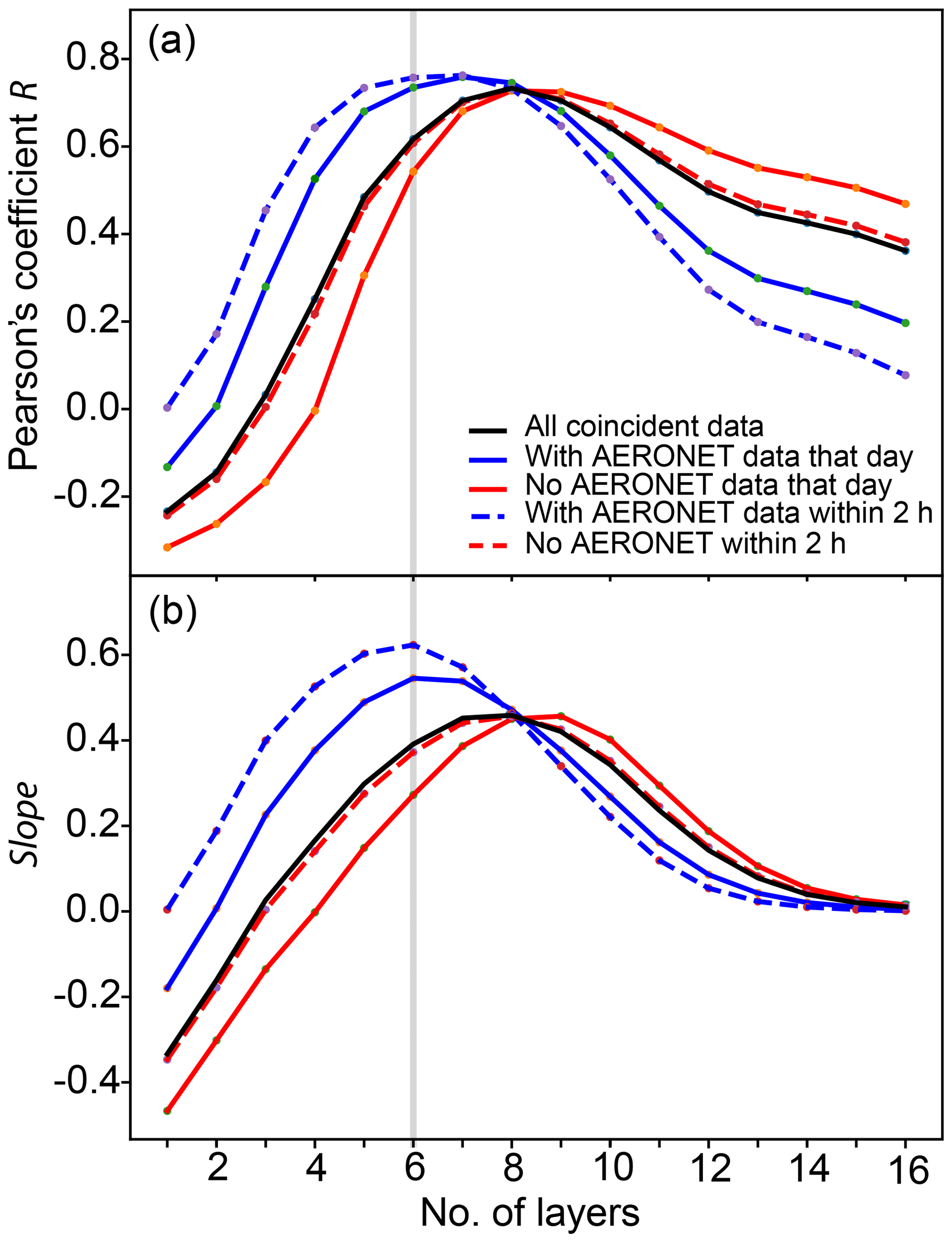
https://www.atmos-meas-tech.net/12/2545/2019/amt-12-2545-2019-f08

Figure 8Pearson's correlation coefficients (a) obtained from hourly surface and MAX-DOAS coincident measurements as a function of the number of layers considered in the VMR averages. The slopes obtained from the linear regressions, performed forcing the intercept to be at zero to the same data sets, are shown in (b). The layers below layer 6 are very likely inside the mixed boundary layer, while layers above layer 6 might be on the edge or above the boundary layer during some hours in the morning (García-Franco et al., 2018). The blue dashed lines only show data when AERONET data are available within 2 h of the scan and hence limit the measurements to cloud-free conditions. This selection criterion improves the correlation significantly.

Download

Generally, a better correlation is found when averaged MAX-DOAS VMRs are compared to in situ surface measurements. Average R values larger than 0.7 are obtained in all cases when the first six to eight layers are considered in the correlation. These correlations decrease rapidly when fewer layers are considered due to increased errors in the lowermost part of the profile. Naturally, the R value also decreases towards a larger number of layers averaged since different air masses are measured at higher altitudes. As expected, slightly larger correlations are obtained for MAX-DOAS retrievals using a measured aerosol input from AERONET (blue traces in Fig. 8), which corresponds to clear-sky conditions.

Linear regressions such as the ones shown in Fig. 9 were generated for each data set, in order to gain more information as to how the number of layers averaged relates to the VMR comparison with the in situ surface measurements. The slope of all coincident data using the first seven to eight layers is 0.45, and it can reach values above 0.6 considering the first six layers in clear-sky conditions (AERONET data available within ±1 h of the measurement time). We thus decide to use the six-layer VMR averages of our MAX-DOAS retrievals in this study, reaching a height of 550 m above the ground level; in the comparisons we present with surface concentrations.

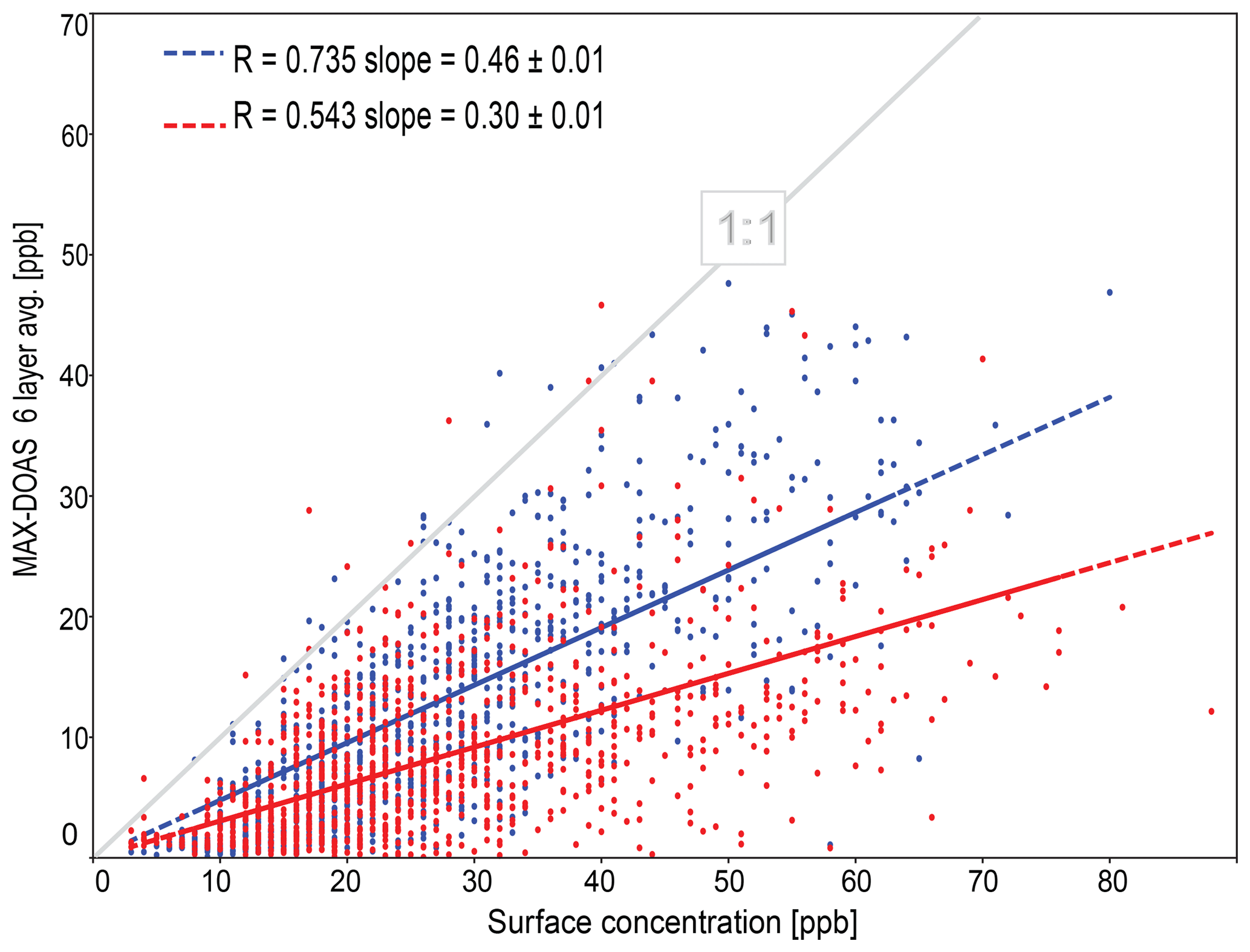
https://www.atmos-meas-tech.net/12/2545/2019/amt-12-2545-2019-f09

Figure 9Correlation plot of the MAX-DOAS six-layer VMR averages vs. the surface measurements shown separately for clear-sky measurements in which aerosol data on that day were available (blue) and for MAX-DOAS retrievals with no aerosol optical depth availability from AERONET, corresponding most likely to cloudy days (red).

Download

To investigate the difference in our data set between clear and cloudy days, a correlation plot is presented in Fig. 9 showing the linear regressions produced from the MAX-DOAS six-layer VMR averages for the retrievals with AERONET availability on that day in blue and those retrievals using a default aerosol a priori profile in red. A significant improvement in the correlation coefficient going from 0.54 to 0.74 is evident in the plot. When all the coincident data are considered, regardless of if the retrieval had data available from the AERONET instrument on that day or not, the R and slope values are 0.62 and 0.39, respectively.

Examples of how the averaged six-layer VMRs and VCD compare to the ground level concentrations on individual days are presented in Fig. 10. These examples were chosen to depict distinct diurnal patterns that occur in different times of the year. Again, the MAX-DOAS six-layer product is consistently lower than the NO₂ concentrations measured at the surface. These, together with the corresponding VCDs plotted on a different y axis, follow the pattern of the surface measurements quite well. The MAX-DOAS instrument captures the features observed at the surface but not without some interesting differences.

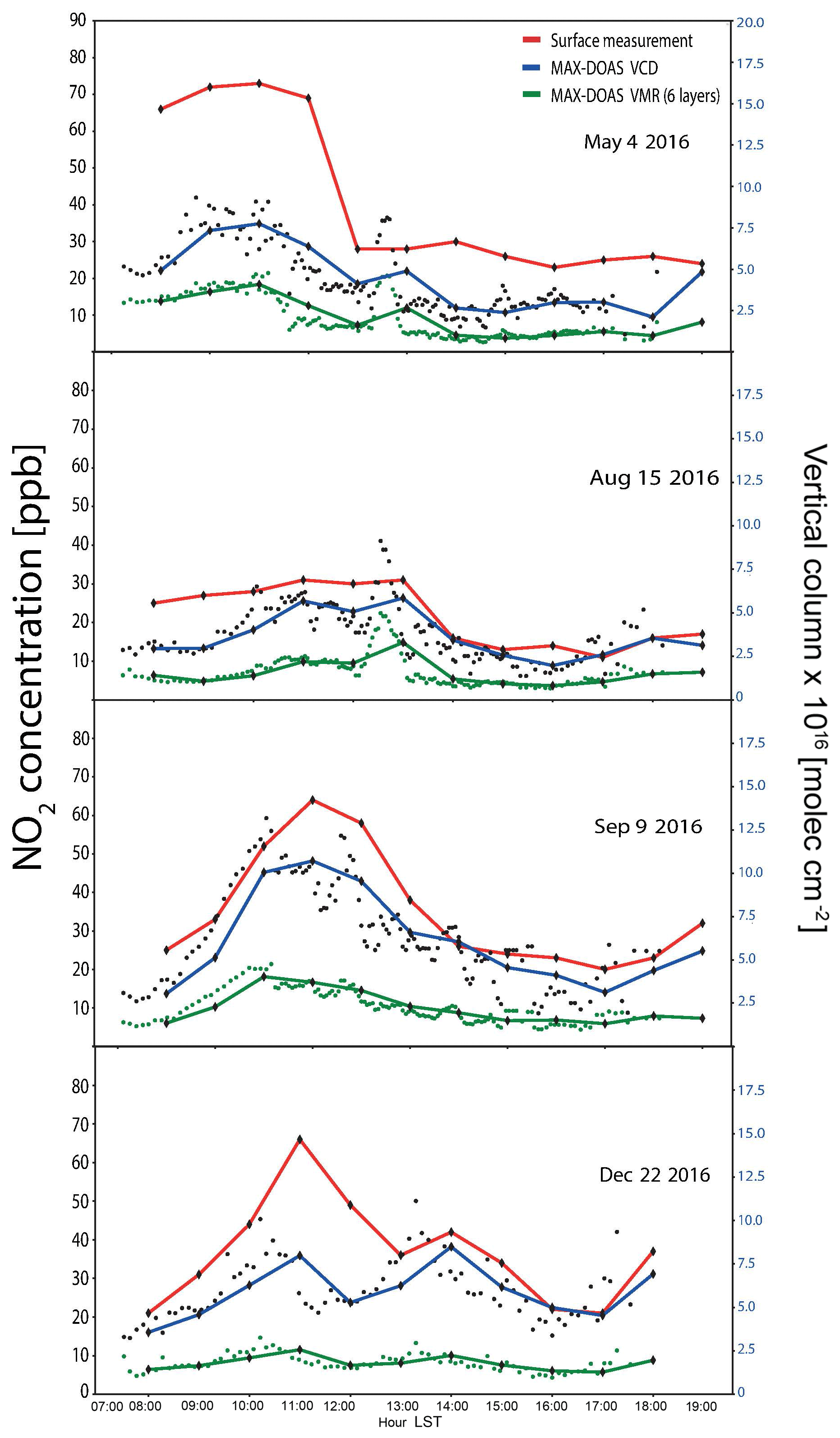
https://www.atmos-meas-tech.net/12/2545/2019/amt-12-2545-2019-f10

Figure 10Example days showing the NO₂ variability in both VMR from the MAX-DOAS (green, <550 m) and surface measurements (red), as well as the total vertical column densities (blue).

Download

https://www.atmos-meas-tech.net/12/2545/2019/amt-12-2545-2019-f11

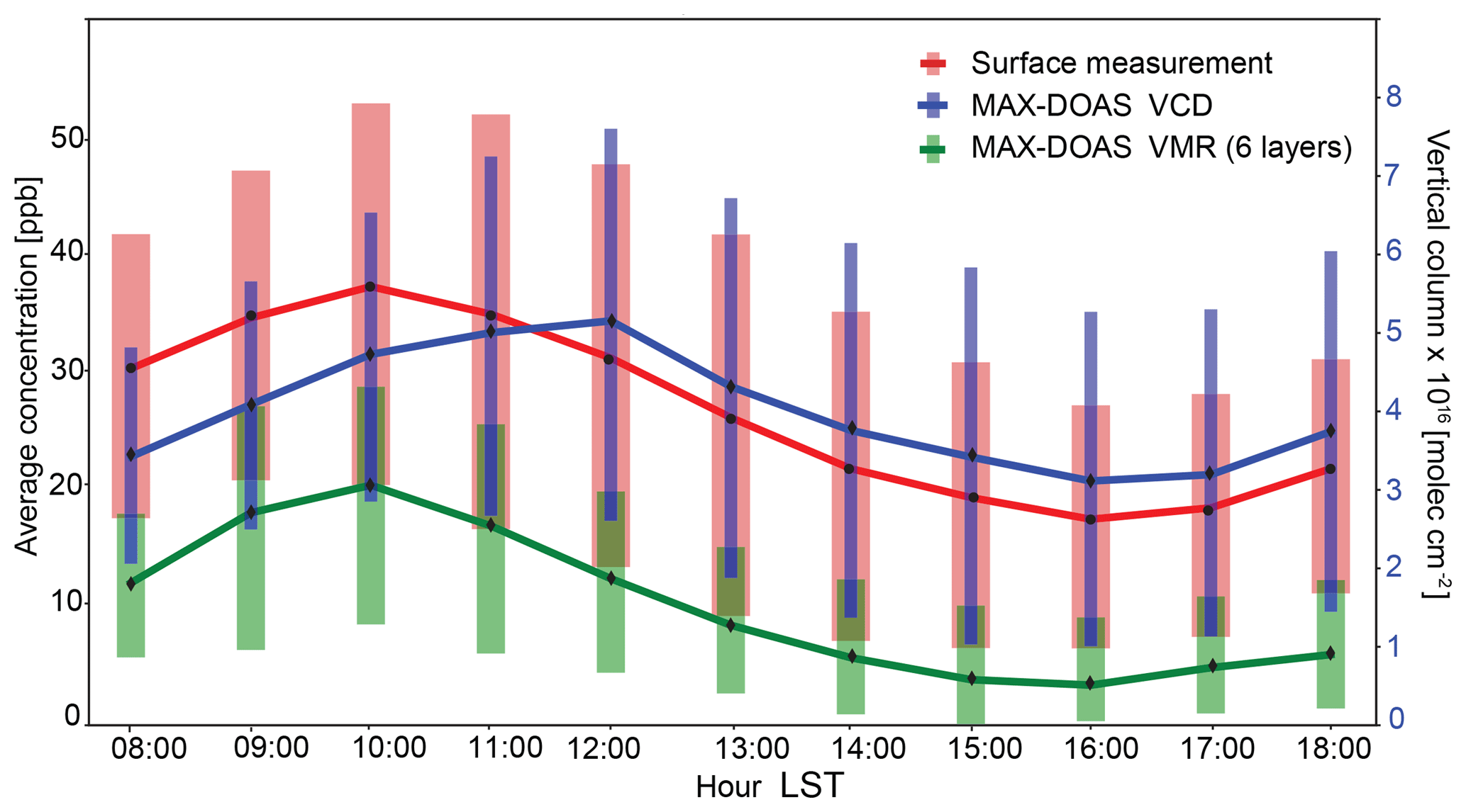
Figure 11Diurnal NO₂ variability from hourly means of the entire data set spanning from January 2015 to July 2016. Only the data with coincident surface and MAX-DOAS measurements are included for consistency in the comparison. Vertical bars correspond to the standard deviations.

Download

https://www.atmos-meas-tech.net/12/2545/2019/amt-12-2545-2019-f12

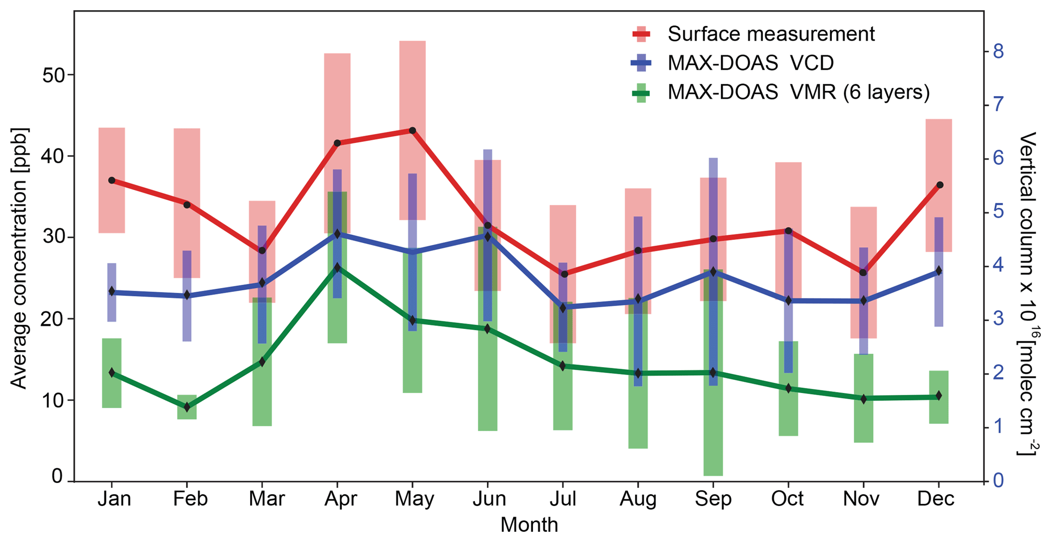
Figure 12Annual NO₂ variability resulting from the monthly mean coincident data (surface and MAX-DOAS) between January 2015 and July 2016. The standard deviations are given in vertical bars.

Download

The data of 4 May 2016 was in the middle of a high-pollution episode in Mexico City, in which a restriction on the use of private vehicles was declared for 4 d. Ozone had surpassed, at least in one of the stations from the monitoring network operated by the city government, the 165 ppb 1 h average concentration. It is interesting to see in the 4 May plot that indeed the surface concentrations of nitrogen dioxide were high in the morning, a condition favoring ozone production, but there is a large NO₂ peak just after noon in the MAX-DOAS VCD and six-layer product data which is not detected at the surface. This is more evident from the individual measurements shown as dots than from the hour averages.

Other differences have to do with the evolution of the mixed layer height, which has been shown to have a rapid growth in the late morning, strongly influencing the surface concentrations (García-Franco et al., 2018). This is for example evident in the 22 December plot, where a peak is observed at 11 h and a second one at 14 h. This peak is strongest at 11 h in the case of the surface measurement, but the total column shows the peak at 14 h to be dominant. The mixed layer has grown in the mean time so that the registered 14 h surface concentration is lower despite there being more NO₂ molecules in the atmosphere.

In order to see the diurnal and seasonal patterns from both MAX-DOAS and surface measurements, all coincident measurements between January 2015 and July 2016 including days with clouds were averaged to a specific hour or month. For consistency, only the coincident 1 h data were considered in order to make the data sets comparable. The mean diurnal evolution with standard deviations as vertical bars is shown in Fig. 11. The maxima of both surface and MAX-DOAS six-layer products are at around 10 h, while that of the vertical column is shifted towards noon. This is expected from what is known from the emissions, growing mixed layer and ventilation patterns in Mexico City (e.g., García-Franco et al., 2018). Despite the fact that the offset in the curves for surface- and MAX-DOAS measurements appears to be nearly constant throughout the day, it would be interesting to investigate further how this offset varies in different seasons, particularly when vertical mixing is not favored.

Figure 12, however, presents the compiled data considered in this study as monthly means in order to observe the seasonal variability and compare the data sets from these two measurement techniques. The three data products coincide in having the highest monthly mean values between April and June. A difference which is probably interesting to note is during December and January, when the concentrations from the surface measurements are relatively higher than those from the MAX-DOAS products. This might have to do with the fact that during these winter months the mixed layer is shallower than during the rest of the year, and the sensitivity of the MAX-DOAS instrument is reduced for the lowest layers as described above.

7 Conclusions

In this contribution we describe the methodology used to analyze the data produced by the network of MAX-DOAS instruments (Arellano et al., 2016) operating in the Mexico City metropolitan area. In general terms, MMF is a retrieval code developed to process the data acquired by the instruments converting the measured spectra together with other input parameters to vertical profiles of aerosols and certain trace gases. We have tested the performance of the code for NO₂ at one of the stations and present some diagnostics and a full error analysis of the results. In the case of NO₂, all error sources amount to about 14.1 %, the smoothing error being the dominating one (12.5 %) followed by the error due to the uncertainties in the aerosol extinction profile (5.1 %).

Both the resulting total vertical column densities and a product consisting of the average VMR in the first six layers (<550 m above the ground level) were compared to ground level NO₂ concentrations. Good correlations were obtained between the six-layer product and the values from the surface measurements, with R values between 0.6 and 0.7. However, the MAX-DOAS systematically underestimates the ground level concentrations by a factor of about 0.6. This is consistent with the total column averaging kernels and variability S_a reported in Sect. 5.1, meaning that the MAX-DOAS instrument has a significantly lower sensitivity near the surface and is most sensitive at a height of around 1 km. It is shown, however, that this underestimation is less for clear-sky conditions as suggested from comparing data when aerosol optical depths were available from independent measurements.

Although results are shown only from one instrument located in the southern part of the city (UNAM), several years of data are available from three other stations at different locations within the metropolitan area (Acatlán, Vallejo and Cuautitlán) that are being analyzed and used for studying the spatial and temporal variability of NO₂ in conjunction with several satellite products.

In this work we present a new and competitive retrieval code which has been developed for retrieving trace gas profiles from MAX-DOAS measurements. Since this study, it has been further improved to perform retrievals in logarithmic space to avoid unphysical negative partial columns and oscillations; it uses the more stable Levenberg–Marquardt iteration scheme and decouples the retrieval and simulation grids⁴.

Further efforts include the improvement in the measurement noise by increasing the integration times during spectral acquisition. This will allow us to improve the retrieval of other gases such as formaldehyde (HCHO) and other weak absorbers. It will also enable us to use OE as a retrieval strategy for aerosol retrieval and possibly increase the DOF to comparable values as for the NO₂ retrieval. This, together with an inclusion of a cloud-screening algorithm in the retrieval chain, will make the retrieval less dependent on the availability of AERONET data.

Data availability

The MAX-DOAS data from the UNAM station can be accessed via http://www.epr.atmosfera.unam.mx/maxdoas_data/no2/nidforval/ (last access: 9 April 2019, Rivera et al., 2019). Data from other stations, with other versions or periods measured within Mexico City's MAX-DOAS network, should be requested from Claudia Rivera (claudia.rivera@atmosfera.unam.mx). Measurements from the surface monitor (CCA station) are performed by Mexico City's Automatic Monitoring Network and can be accessed via http://www.aire.cdmx.gob.mx/ (last access: 9 April 2019).

Appendix A

In a recent update of the code, implemented after the analysis presented here (i.e., not used for obtaining the results here), the retrieval space was changed from linear space to logarithmic retrieval space. This means that the retrieval works in a linear (dSCD measurement) and logarithmic (profile retrieval) space now. This enhances the nonlinearity of the problem and requires a change of iteration scheme. The GN iteration scheme (Eq. 1) is replaced by a slightly slower but more stable Levenberg–Marquardt (LM) iteration scheme; i.e., Eq. (1) is replaced by Eq. (A1) for more nonlinear inversion problems (Rodgers, 2000).

\begin{array}{l} (A1) & x_{i + 1} = & x_{i} + {[(1 + γ) R + K_{i}^{T}] S_{m}^{- 1} K_{i}]}^{- 1} \\ [K_{i}^{T} S_{m}^{- 1} (y - F (x_{i})) - R (x_{i} - x_{a})] \end{array}

The symbols mean the same as in Eq. (1): superscript “T” denotes transposed, superscript “−1” denotes the inverse and subscript “a” indicates a priori values. S_m is the measurement error covariance matrix, y denotes the vector of measured differential slant column densities, F(x_i) denotes the simulated differential slant column densities at iteration i, calculated using the forward model with input profile x_i, and K_i is the Jacobian matrix at the ith iteration.

The new x_i+1 in Eq. (A1) is only accepted if the cost function in Eq. (A2) decreases with respect to the cost function of the previous iteration.

\begin{array}{l} (A2) & cost = & \sum_{k}^{angles} \sum_{j}^{angles} (y - F (x))_{k} {S_{m}^{- 1}}^{k j} (y - F (x))_{j} \\ + \sum_{k}^{layers} \sum_{j}^{layers} (x - x_{a})_{k} S {a^{- 1}}^{k j} (x - x_{a})_{j} \end{array}

If this is the case, x_i+1 is accepted and if (1+γ) is not yet equal to 1, the factor (1+γ) is halved for the next iteration. If, however, the cost function increases, the newly calculated x_i+1 is discarded and the ith calculation repeated with a factor (1+γ) increased by a factor of 16.

In order to counteract the slowdown of the retrieval, more restrictions were placed on the observation geometry for a single scan: a single relative azimuth angle and a single solar zenith angle per scan. This means in particular that two different viewing directions cannot be treated as a single scan any longer. Also, it is no longer necessary to have the full simulation grid as the retrieval grid. The retrieval can be limited to the lower part of the simulation grid. Although the former change (with respect to observation geometry) means a significant cut in flexibility, it results in a retrieval time speed up of a factor of 4, and a more typical retrieval time per scan and per constituent (i.e., for both aerosol and trace gas) is around 5 s.

Tests using the logarithm of the partial layer vertical column density (for NO₂ retrieval) or layer extinction profile (for aerosol retrieval) motivated the change to the LM iteration scheme due to the increased nonlinearity when working in a semi-log space as state-measurement space. With this new configuration, MMF has been participating in the round robin comparison of different retrieval codes for the FRM₄DOAS project (Frieß et al., 2018). It has also participated in the profile retrieval from dSCD from the CINDI-2 campaign, both for NO₂ and HCHO (Tirpitz et al., 2019).

If the retrieval is to be performed in log space, i.e., to work with ln (x) instead of with x as the retrieval parameter, K in Eq. (16) is multiplied by x (since the raw output from VLIDORT is Kx, no division by x is necessary because the quantity needed in logarithmic space is Kx) and the uncertainty covariance matrix S_a in Eq. (A1) needs to be left and right multiplied by 1∕x.

The LM scheme of Eq. (A1) has currently only been tested with OE and not with Tikhonov regularization; i.e., the aerosol retrieval was also performed using OE.

Appendix B: Calculations for dry air density

In this appendix, we outline the calculation of Z, the molar mass of air M_a and the depolarization ratio Δ. We follow Ciddor (1996). If T is given in kelvin (temperature in degrees Celsius is denoted as T_C), σ the wavenumber per micrometer, pressure P in pascals and volume mixing ratio of CO₂ in parts per million, the constants in Eqs. (B1)–(B14) have the following values.

\begin{array}{llr} k_{0} & = & 238.0185 \\ a_{0} & = & 1.58123 \times 10^{- 6} \\ b_{0} & = & 5.707 \times 10^{- 6} \\ w_{0} & = & 295.235 \\ k_{1} & = & 5792105.0 \\ a_{1} & = & - 2.9331 \times 10^{- 8} \\ b_{1} & = & - 2.051 \times 10^{- 8} \\ w_{1} & = & 2.6422 \\ k_{2} & = & 57.362 \\ a_{2} & = & 1.1043 \times 10^{- 10} \\ c_{0} & = & 1.9898 \times 10^{- 4} \\ w_{2} & = & - 0.03238 \\ k_{3} & = & 167917.0 \\ α & = & 1.00062 \\ c_{1} & = & - 2.376 \times 10^{- 6} \\ w_{3} & = & 0.004028 \\ d & = & 1.83 \times 10^{- 11} \\ β & = & 3.14 \times 10^{- 8} \\ A & = & 1.2379 \times 10^{- 5} \\ C & = & 33.937 \\ e & = & - 0.765 \times 10^{- 8} \\ γ & = & 5.6 \times 10^{- 7} \\ B & = & - 1.912 \times 10^{- 2} \\ D & = & - 6.343 \times 10^{3} \end{array}

First, the saturation vapor pressure 𝒮 is calculated according to Eq. (B1), then the enhancement factor for water vapor in air, ℱ, is calculated according to Eq. (B2) and with this, the molar fraction of water vapor in moist air x_w is calculated according to Eq. (B3), where P_w is partial water vapor pressure in pascals.

\begin{array}{l} (B1) & S = \exp (A T^{2} + B T + C + D / T) \\ (B2) & F = α + β P + γ T_{C}^{2} \\ (B3) & x_{w} = F P_{w} / P \end{array}

The air density in dry air $n_{air, dry, 450}$ (0 % humidity) at standard conditions (15 ^∘C, 101.325 Pa, xCO₂=450 ppm) can be calculated as in Eq. (B4) and from this the dry air density at xCO₂ is calculated according to Eq. (B5).

\begin{matrix} (B4) & (n_{air, dry, 450} - 1) \times 10^{8} = \frac{k_{1}}{k_{0} - σ^{2}} + \frac{k_{3}}{k_{2} - σ^{2}} \end{matrix}

\begin{array}{l} (B5) & (n_{air, dry, {x CO}_{2}} - 1) = & (n_{air, dry, 450} - 1) \times 10^{8} \\ (1.0 + 0.534 \times 10^{- 6} \cdot (x {CO}_{2} - 450.0)) \end{array}

The equivalent quantity for water vapor, n_wv, is calculated as follows:

\begin{matrix} (B6) & n_{wv} = 1.022 \cdot (w_{0} + w_{1} σ^{2} + w_{2} σ^{4} + w_{3} σ^{6}) . \end{matrix}

The molar mass of dry air, M_a, with xCO₂ is calculated as

\begin{matrix} (B7) & M_{a} = 10^{- 3} (28.9635 + 12.011 \times 10^{- 6} (x {CO}_{2} - 400.0)) . \end{matrix}

The compressibility of dry air, Z_a, and pure water vapor, Z_w, are calculated as

\begin{array}{l} (B8) & Z_{a} = & 1.0 - \frac{101325.0}{288.15} (a_{0} + 15 a_{1} + 225 a_{2}), \\ (B9) & Z_{w} = & 1.0 - \frac{1333.0}{293.15} (a_{0} + 20 a_{1} + 400 a_{2} + b_{0} \\ + 20 b_{1} + c_{0} + 20 c_{1}) + {(\frac{1333.0}{293.15})}^{2} (d + e) . \end{array}

Using Eq. (B10) once with the values for Z, R and T for standard water vapor and once with the values for standard air, one can calculate ρ_ws and ρ_axs, respectively.

\begin{matrix} (B10) & ρ = (p M_{a} / (Z R_{gas} T) (1 - x_{w} (1 - M_{mwv} / M_{a})) \end{matrix}

Here, R_gas=8.3144621 J mol⁻¹ K⁻¹ is the gas constant and M_mwv=0.018015 kg mol⁻¹ is the molar mass of water vapor. Z, the compressibility of moist air at T, x_w and P can be calculated as

\begin{array}{l} (B11) & Z = & 1.0 - (P / T) (a_{0} + a_{1} T_{C} + a_{2} T_{C}^{2} + (b_{0} + b_{1} T_{C}) x_{w} \\ + (c_{0} + c_{1} T_{C}) x_{w}^{2}) + (P / T)^{2} (d + e x_{w}^{2}) . \end{array}

Using again Eq. (B10), with the actual values for P, x_w and Z, the density of the dry air component can be calculated according to Eq. (B12) and the density of the water vapor component can be calculated according to Eq. (B13).

\begin{array}{l} (B12) & ρ_{dryair} = P M_{a} (1 - x_{w}) / (Z R_{gas} T) \\ (B13) & ρ_{wv} = P M_{mwv} x_{w} / (Z R_{gas} T) \end{array}

Finally, the number density of the air ρ and the refractive index n are calculated as

\begin{array}{l} (B14) & ρ = \frac{ρ_{dryair}}{M_{a}} Av, \\ (B15) & n = \frac{ρ_{dryair}}{ρ_{axs}} (n_{air,dry, x {CO}_{2}} - 1) + \frac{ρ_{wv}}{ρ_{ws}} (n_{wv} - 1) . \end{array}

Here, $Av = 6.02214129 \times 10^{23}$ is the Avogadro number.

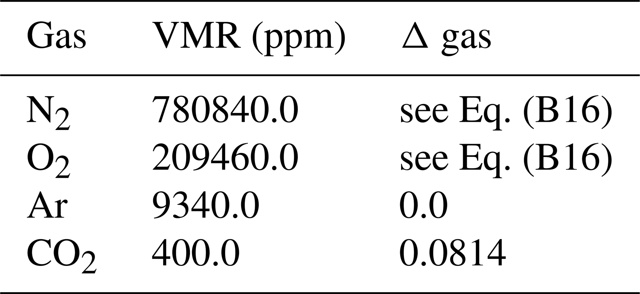
We use the N₂, O₂ and CO₂ depolarization factors from Bates (1984) and fixed VMR as summarized in Table B1 and calculate the wavelength-dependent depolarization factor via Eq. (B16), where F is the so-called King factor and is calculated for N₂ (λ in micrometers) and O₂ according to Eqs. (B18) and (B19), respectively. The complete depolarization factor is then calculated according to Eq. (B19).

Table B1Depolarization ratios and VMR for main air constituents

Download Print Version | Download XLSX

\begin{array}{l} (B16) & Δ = 6.0 \cdot (1 - F) / (- 7 F - 3) \\ (B17) & F (N_{2}) = 1.034 + 3.17 \times 10^{- 4} / λ^{2} \\ (B18) & F (O_{2}) = 1.096 + 1.385 \times 10^{- 3} / λ^{2} \\ + 1.448 \times 10^{- 4} / λ^{4} \\ (B19) & Δ = \sum (Δ_{i} {VMR}_{i}), i = N_{2}, O_{2}, Ar, {CO}_{2} \end{array}

For the Rayleigh scattering cross section, we implement Eq. (7.37) from Goody and Yung (1989) and Eq. (19.5) from Platt et al. (2007); see Eq. (B20).

\begin{matrix} (B20) & Q_{Ray} = \frac{24 π^{3} (n^{2} - 1)^{2}}{λ^{4} ρ^{2} (n^{2} + 2)^{2}} \frac{6 + 3 Δ}{6 - 7 Δ} \end{matrix}

Author contributions

MMF is responsible for the retrieval code development and testing, the retrieval chain setup from spectra to profiles, and the retrieval parameter choices for MMF and software support. In terms of text contributions, MMF wrote Sect. 4, Appendix A and B and part of the abstract and Sect. 1. MMF produced Figs. 1–3. CR is responsible for the QDOAS retrieval setup and parameter choices. CR wrote Sect. 3 and parts of Sect. 2. WS and ZO are responsible for the data analysis and interpretation, as well as for the sensitivity tests and the error analysis. They wrote Sect. 5 and parts of Sects. 6 and 7. They produced Figs. 4–12. JA constructed and installed the instruments and was responsible for their maintenance. JA wrote Sect. 2. AB provided technical support for instruments and data management. JAGR provided the WRF-Chem simulations that serve as a priori data for NO₂ retrieval. JAGR wrote parts of Sect. 4.2.1. MG was involved in the data analysis and interpretation and wrote Sect. 7 and parts of Sects. 1 and 6.

Competing interests

The authors declare that they have no conflict of interest.

Acknowledgements

We would like to thank the financial support provided by CONACYT (grants 275239 and 290589) and DGAPA-UNAM (grants IN107417, IN111418, and IA100716 and Martina M. Friedrich's postdoctoral fellowship). SEDEMA is acknowledged for providing the in situ surface concentrations from their monitoring network (RAMA) as well for partially supporting the MAX-DOAS network, and Arne Krueger, Alfredo Rodríguez, Hector Soto and Delibes Flores are thanked for their technical assistance. We thank Caroline Fayt (caroline.fayt@aeronomie.be), Michel Van Roozendael (michelv@aeronomie.be) and Thomas Danckaert for the free use of the QDOAS software and we thank Robert Spurr for free use of the VLIDORT radiative transfer code package. We thank the Mexican Solarimetric Service for their effort in establishing and maintaining the AERONET Mexico City site. We thank the University of Wyoming Department of Atmospheric Science for providing the sounding data on http://weather.uwyo.edu/upperair/sounding.html (last access: 9 April 2019).

This research has been supported by the CONACYT (grant no. 275239), the CONACYT (grant no. 290589), the DGAPA-UNAM (grant no. IN107417), the DGAPA-UNAM (grant no. IN111418) and the DGAPA-UNAM (grant no. IA100716).

Review statement

This paper was edited by Lok Lamsal and reviewed by three anonymous referees.

References

Arellano, J., Krüger, A., Rivera, C., Stremme, W., Friedrich, M., Bezanilla, A., and Grutter, M.: The MAX-DOAS network in Mexico City to measure atmospheric pollutants, Atmosfera, 29, 157–167, 2016. a, b, c, d, e

Bates, D. R.: Rayleigh scattering by air, Planet. Space Sci., 32, 785–790, https://doi.org/10.1016/0032-0633(84)90102-8, 1984. a, b

Buchwitz, M., Rozanov, V. V., and Burrows, J. P.: Development of a correlated-k distribution band model scheme for the radiative transfer program GOMETRAN/SCIATRAN for retrieval of atmospheric constituents from SCIMACHY/ENVISAT-1 data, Proc. SPIE, 3495, Satellite Remote Sensing of Clouds and the Atmosphere III, https://doi.org/10.1117/12.332681, 1998. a

Burrows, J. P., Richter, A., Dehn, A., Deters, B., Himmelmann, S., Voigt, S., and Orphal, J.: Atmospheric remote-sensing reference data from GOME. 2. Temperature dependent absorption cross sections of O₃ in the 231-794 nm range, J. Quant. Spectrosc. Ra., 61, 509–517, https://doi.org/10.1016/S0022-4073(98)00037-5, 1999. a, b

Carlson, D., Donohoue, D., Platt, U., and Simpson, W. R.: A low power automated MAX-DOAS instrument for the Arctic and other remote unmanned locations, Atmos. Meas. Tech., 3, 429–439, https://doi.org/10.5194/amt-3-429-2010, 2010. a

Ciddor, P. E.: Refractive index of air: new equations for the visible and near infrared, Appl. Opt., 35, 1566, https://doi.org/10.1364/AO.35.001566, 1996. a

Coburn, S., Dix, B., Sinreich, R., and Volkamer, R.: The CU ground MAX-DOAS instrument: characterization of RMS noise limitations and first measurements near Pensacola, FL of BrO, IO, and CHOCHO, Atmos. Meas. Tech., 4, 2421–2439, https://doi.org/10.5194/amt-4-2421-2011, 2011. a

Dahlback, A. and Stamnes, K.: A new spherical model for computing the radiation field available for photolysis and heating at twilight, Planet. Space Sci., 39, 671–683, https://doi.org/10.1016/0032-0633(91)90061-E, 1991. a

Danckaert, T., Fayt, C., Van Roozendael, M., De Smedt, I., Letocart, V., Merlaud, A., and Pinardi, G.: QDOAS Software user manual, Belgian Institute for Space Aeronomy, 2013. a, b, c, d, e

Finlayson-Pitts, B. J. and Pitts, J. N.: Chemistry of the upper and lower atmosphere: theory, experiments, and applications, Academic Press, San Diego, CA, 2000. a

Frieß, U., Monks, P. S., Remedios, J. J., Rozanov, A., Sinreich, R., Wagner, T., and Platt, U.: MAX-DOAS O₄ measurements: A new technique to derive information on atmospheric aerosols: 2. Modeling studies, J. Geophys. Res.-Atmos., 111, D14203, https://doi.org/10.1029/2005JD006618, 2006. a

Frieß, U., Beirle, S., Alvarado Bonilla, L., Bösch, T., Friedrich, M. M., Hendrick, F., Piters, A., Richter, A., van Roozendael, M., Rozanov, V. V., Spinei, E., Tirpitz, J.-L., Vlemmix, T., Wagner, T., and Wang, Y.: Intercomparison of MAX-DOAS Vertical Profile Retrieval Algorithms: Studies using Synthetic Data, Atmos. Meas. Tech. Discuss., https://doi.org/10.5194/amt-2018-423, in review, 2018. a

Galle, B., Johansson, M., Rivera, C., Zhang, Y., Kihlman, M., Kern, C., Lehmann, T., Platt, U., Arellano, S., and Hidalgo, S.: Network for Observation of Volcanic and Atmospheric Change (NOVAC) A global network for volcanic gas monitoring: Network layout and instrument description, J. Geophys. Res., 115, D05304, https://doi.org/10.1029/2009JD011823, 2010. a

García-Franco, J., Stremme, W., Bezanilla, A., Ruiz-Angulo, A., and Grutter, M.: Variability of the Mixed-Layer Height Over Mexico City, Bound.-Lay. Meteorol., 167, 493–507, https://doi.org/10.1007/s10546-018-0334-x, 2018. a, b, c, d, e

Goody, R. M. and Yung, Y. L.: Atmospheric radiation: theoretical basis, Oxford University Press, 1989. a, b

Hendrick, F., Müller, J.-F., Clémer, K., Wang, P., De Mazière, M., Fayt, C., Gielen, C., Hermans, C., Ma, J. Z., Pinardi, G., Stavrakou, T., Vlemmix, T., and Van Roozendael, M.: Four years of ground-based MAX-DOAS observations of HONO and NO2 in the Beijing area, Atmos. Chem. Phys., 14, 765–781, https://doi.org/10.5194/acp-14-765-2014, 2014. a

Hermans, C., Vandaele, A. C., Carleer, M., Fally, S., Colin, R., Jenouvrier, A., Coquart, B., and Mérienne, M. F.: Absorption cross-sections of atmospheric constituents: NO₂, O₂, and H₂O, Environ. Sci. Pollut. Res., 6, 151–158, 1999. a, b

Hess, M., Koepke, P., and Schult, I.: Optical Properties of Aerosols and Clouds: The Software Package OPAC., B. Am. Meteorol. Soc., 79, 831–844, https://doi.org/10.1175/1520-0477(1998)079<0831:OPOAAC>2.0.CO;2, 1998. a

Hönninger, G., Bobrowski, N., Palenque, E. R., Torrez, R., and Platt, U.: Reactive bromine and sulfur emissions at Salar de Uyuni, Bolivia, J. Geophys. Res. Lett., 31, L04101, https://doi.org/10.1029/2003GL018818, 2004. a, b

Johansson, M., Rivera, C., de Foy, B., Lei, W., Song, J., Zhang, Y., Galle, B., and Molina, L.: Mobile mini-DOAS measurement of the outflow of NO₂ and HCHO from Mexico City, Atmos. Chem. Phys., 9, 5647–5653, https://doi.org/10.5194/acp-9-5647-2009, 2009. a

Kirmse, B., Delon, A., and Jost, R.: NO₂ absorption cross section and its temperature dependence, J. Geophys. Res., 102, 16089–16098, https://doi.org/10.1029/97JD00075, 1997. a

Kurucz, R. L., Furenlid, I., Brault, J., and Testerman, L.: Solar flux atlas from 296 to 1300 nm, National Solar Observatory Atlas No. 1, 1984. a

Marquard, L.: Modellierung des Strahlungstransports in der Erdatmosphäre für absorptionsspektroskopische Messungen im ultravioletten und sichtbaren Spektralbereich, Logos Verlag, Berlin, ISBN 3897220520, 1998. a

Marquard, L. C., Wagner, T., and Platt, U.: Improved air mass factor concepts for scattered radiation differential optical absorption spectroscopy of atmospheric species, J. Geophys. Res., 105, 1315–1327, https://doi.org/10.1029/1999JD900340, 2000. a

Melamed, M. L., Basaldud, R., Steinbrecher, R., Emeis, S., Ruíz-Suárez, L. G., and Grutter, M.: Detection of pollution transport events southeast of Mexico City using ground-based visible spectroscopy measurements of nitrogen dioxide, Atmos. Chem. Phys., 9, 4827–4840, https://doi.org/10.5194/acp-9-4827-2009, 2009. a

Meller, R. and Moortgat, G. K.: Temperature dependence of the absorption cross sections of formaldehyde between 223 K and 323 K in the wavelength range 225–375 nm, J. Geophys. Res., 105, 7089–7101, 2000. a

Molina, L. T. and Molina, M. J.: Air quality in the Mexico megacity: an integrated assessment, Kluwer Academic Publishers, Dordrecht, Boston, 2002. a

Orphal, J.: A critical review of the absorption cross-sections of O₃ and NO₂ in the ultraviolet and visible, J. Photoch. Photobio. A, 157, 185–209, https://doi.org/10.1016/S1010-6030(03)00061-3, 2002. a

Ortega, I., Koenig, T., Sinreich, R., Thomson, D., and Volkamer, R.: The CU 2-D-MAX-DOAS instrument – Part 1: Retrieval of 3-D distributions of NO₂ and azimuth-dependent OVOC ratios, Atmos. Meas. Tech., 8, 2371–2395, https://doi.org/10.5194/amt-8-2371-2015, 2015. a

Palazzi, E., Petritoli, A., Giovanelli, G., Kostadinov, I., Bortoli, D., Ravegnani, F., and Sackey, S. S.: PROMSAR: A backward Monte Carlo spherical RTM for the analysis of DOAS remote sensing measurements, Adv. Space Res., 36, 1007–1014, https://doi.org/10.1016/j.asr.2005.05.017, 2005. a

Perliski, L. M. and Solomon, S.: On the evaluation of air mass factors for atmospheric near-ultraviolet and visible absorption spectroscopy, J. Geophys. Res., 98, 10363, https://doi.org/10.1029/93JD00465, 1993. a

Platt, U. and Stutz, J.: Differential Optical Absorption Spectroscopy, Springer-Verlag Berlin Heidelberg, https://doi.org/10.1007/978-3-540-75776-4, 2008. a, b

Platt, U., Pfeilsticker, K., and Vollmer, M.: Radiation and Optics in the Atmosphere, Springer Handbook of Lasers and Optics, p. 1165, https://doi.org/10.1007/978-0-387-30420-5_19, 2007. a, b

Rahpoe, N., von Savigny, C., Weber, M., Rozanov, A. V., Bovensmann, H., and Burrows, J. P.: Error budget analysis of SCIAMACHY limb ozone profile retrievals using the SCIATRAN model, Atmos. Meas. Tech., 6, 2825–2837, https://doi.org/10.5194/amt-6-2825-2013, 2013a. a

Rivera, C., Barrera, H., Grutter, M., Zavala, M., Galle, B., Bei, N., Li, G., and Molina, L. T.: NO₂ fluxes from Tijuana using a mobile mini-DOAS during Cal-Mex 2010, Atmos. Environ., 70, 532–539, https://doi.org/10.1016/j.atmosenv.2012.12.026, 2013. a

Rivera, C., Stremme, W., Ojeda, Z., Bezanilla, A., Arellano, J., Friedrich, M. M., and Grutter, M.: NO₂ profiles from MAXDOAS measurements at UNAM station, available at: http://www.epr.atmosfera.unam.mx/maxdoas_data/no2/nidforval/, last access: 9 April 2019. a

Rodgers, C. D.: Inverse Methods for Atmospheric Sounding: Theory and Practice, Series on Atmospheric, Oceanic and Planetary Physics, Vol. 2, World Scientific Publishing Co, 256 pp., https://doi.org/10.1142/3171, 2000. a, b, c, d, e

Rodgers, C. D. and Connor, B. J.: Intercomparison of remote sounding instruments, J. Geophys. Res.-Atmos., 108, 4116, https://doi.org/10.1029/2002JD002299, 2003. a

Rozanov, V. V., Rozanov, A. V., Kokhanovsky, A. A., and Burrows, J. P.: Radiative transfer through terrestrial atmosphere and ocean: Software package SCIATRAN, J. Quant. Spectrosc. Ra., 133, 13–71, https://doi.org/10.1016/j.jqsrt.2013.07.004, 2014. a

Rozanov, V. V., Dinter, T., Rozanov, A. V., Wolanin, A., Bracher, A., and Burrows, J. P.: Radiative transfer modeling through terrestrial atmosphere and ocean accounting for inelastic processes: Software package SCIATRAN, J. Quant. Spectrosc. Ra., 194, 65–85, https://doi.org/10.1016/j.jqsrt.2017.03.009, 2017. a

Spurr, R.: VLIDORT: A linearized pseudo-spherical vector discrete ordinate radiative transfer code for forward model and retrieval studies in multilayer multiple scattering media, J. Quant. Spectrosc. Ra., 102, 316–342, 2006. a, b

Spurr, R.: User's Guide VLIDORT Version 2.6, RT Solutions, Inc., 2013. a, b, c

Spurr, R. J. D., Kurosu, T. P., and Chance, K. V.: A linearized discrete ordinate radiative transfer model for atmospheric remote-sensing retrieval, J. Quant. Spectrosc. Ra., 68, 689–735, https://doi.org/10.1016/S0022-4073(00)00055-8, 2001. a, b, c

Stamnes, K., Tsay, S.-C., Jayaweera, K., and Wiscombe, W.: Numerically stable algorithm for discrete-ordinate-method radiative transfer in multiple scattering and emitting layered media, Appl. Opt., 27, 2502–2509, https://doi.org/10.1364/AO.27.002502, 1988. a

Steck, T.: Methods for determining regularization for atmospheric retrieval problems, Appl. Opt., 41, 1788–1797, https://doi.org/10.1364/AO.41.001788, 2002. a

Tirpitz, J.-L., Frieß, U., Hendrick, F., Alberti, C., Allaart, M., Apituley, A., Bais, A., Beirle, S., Benavent, N., Berkhout, S., Bösch, T., Bognar, K., Bruchkouski, I., Chan, K. L., Chengxin, Z., den Hoed, M., Donner, S., Drosoglou, T., Friedrich, M. M., Frumau, A., Gast, L., Gomez, L., Gielen, C., Hao, N., Hensen, A., Henzing, B., Hoque, S., Irie, H., Jin, J., Koenig, T. K., Kreher, K., Kuhn, J., Kumar, V., Lampel, J., Li, A., Liu, C., Ma, J., Merlaud, A., Mishra, A., Nieto, D., Peters, E., Pinardi, G., Piters, A., Pöhler, D., Postylyakov, O., Richter, A., van Roozendael, M., Schmitt, S., Sinha, V., Spinei, E., Stein, D., Swart, D., Tack, F., Vlemmix, T., van der Hoff, R., Vonk, J., Wagner, T., Wang, S., Wang, Y., Wang, Z., Wenig, M., Wiegner, M., Wittrock, F., Xie, P., Xing, C., Xu, J., and Zhao, X.: DOAS Vertical Profile Retrieval Algorithms: Studies on Field Data from the CINDI-2 Campaign, Atmos. Meas. Tech., in preparation, 2019. a

Vandaele, A. C., Hermans, C., Simon, P. C., Carleer, M., Colin, R., Fally, S., Mérienne, M. F., Jenouvrier, A., and Coquart, B.: Measurements of the NO₂ absorption cross-section from 42 000 cm⁻¹ to 10 000 cm⁻¹ (238–1000 nm) at 220 K and 294 K, J. Quant. Spectrosc. Ra., 59, 171–184, 1998. a, b

Vandaele, A. C., Hermans, C., Fally, S., Carleer, M., Merienne, M.-F., Jenouvrier, A., Coquart, B., and Colin, R.: Absorption cross-sections of NO₂: simulation of temperature and pressure effects, J. Quant. Spectrosc. Ra., 76, 373–391, https://doi.org/10.1016/S0022-4073(02)00064-X, 2003. a

Vidot, J., Jourdan, O., Kokhanosvky, A. A., Szczap, F., Giraud, V., and Rozanov, V. V.: Retrieval of tropospheric NO₂ columns from satellite measurements in presence of cirrus: A theoretical sensitivity study using SCIATRAN and prospect application for the A-Train, J. Quant. Spectrosc. Ra., 111, 586–601, 2010. a

von Friedeburg, C.: Derivation of Trace Gas Information combining Differential Optical Absorption Spectroscopy with Radiative Transfer Modelling, PhD thesis, Ruperto-Carola University of Heidelberg, Germany, 2003. a

von Friedeburg, C., Wagner, T., Geyer, A., Kaiser, N., Vogel, B., Vogel, H., and Platt, U.: Derivation of tropospheric NO₃ profiles using off-axis differential optical absorption spectroscopy measurements during sunrise and comparison with simulations, J. Geophys. Res.-Atmos., 107, 4168, https://doi.org/10.1029/2001JD000481, 2002. a

Wagner, T., Beirle, S., Brauers, T., Deutschmann, T., Frieß, U., Hak, C., Halla, J. D., Heue, K. P., Junkermann, W., Li, X., Platt, U., and Pundt-Gruber, I.: Inversion of tropospheric profiles of aerosol extinction and HCHO and NO₂ mixing ratios from MAX-DOAS observations in Milano during the summer of 2003 and comparison with independent data sets, Atmos. Meas. Tech., 4, 2685–2715, https://doi.org/10.5194/amt-4-2685-2011, 2011. a

Wang, S., Cuevas, C. A., Frieß, U., and Saiz-Lopez, A.: MAX-DOAS retrieval of aerosol extinction properties in Madrid, Spain, Atmos. Meas. Tech., 9, 5089–5101, https://doi.org/10.5194/amt-9-5089-2016, 2016. a

Wang, Y., Lampel, J., Xie, P., Beirle, S., Li, A., Wu, D., and Wagner, T.: Ground-based MAX-DOAS observations of tropospheric aerosols, NO₂, SO₂ and HCHO in Wuxi, China, from 2011 to 2014, Atmos. Chem. Phys., 17, 2189–2215, https://doi.org/10.5194/acp-17-2189-2017, 2017. a, b, c, d, e, f, g, h

Wilmouth, D. M., Hanisco, T. F., Donaue, N. M., and Anderson, J. G.: Fourier Transform Ultraviolet Spectroscopy of the $A^{2} \prod_{3 / 2} \leftarrow X^{2} \prod_{3 / 2}$ , J. Phys. Chem. A, 103, 8935–8945, 1999. a

Wittrock, F., Oetjen, H., Richter, A., Fietkau, S., Medeke, T., Rozanov, A., and Burrows, J. P.: MAX-DOAS measurements of atmospheric trace gases in Ny-Ålesund – Radiative transfer studies and their application, Atmos. Chem. Phys., 4, 955–966, https://doi.org/10.5194/acp-4-955-2004, 2004. a

In a recent update, the GN scheme was replaced by the more stable Levenberg–Marquardt (LM) iteration scheme; more details on recent changes can be found in Appendix A.

We only use the LIDORT part of VLIDORT, meaning that we only consider the total intensity and not the polarization.

Bulk property that does not change when changing the size of the system.

⁴

Details can be found in Appendix A.

Articles

Short summary

We present a new numerical code to retrieve NO₂ vertical column densities (VCDs) and concentrations from previously retrieved slanted columns from spectroscopic measurements in the visible and ultraviolet spectral ranges in different vertical viewing directions. We use this code on 1.5 years of data from a measurement station located in the south of Mexico City and compare daily and monthly averages to averages of in situ measurements. We show daily NO₂ VCD time series for a few example days.

NO2 vertical profiles and column densities from MAX-DOAS measurements in Mexico City

2.1 The scanner

2.2 The acquisition–control unit

2.3 Measurement strategy

4.1 Inversion theory

4.2 Forward model

4.2.1 Input for gases

4.2.2 Input for aerosols

4.2.3 Calculating final VLIDORT input

4.3 Calculating dSCDs and weighting functions

5.1 Smoothing error

5.2 Measurement noise

5.3 Parameter errors

5.3.1 Parameter error from spectroscopy

5.3.2 Parameter error from aerosol profile

5.4 Forward model error

5.5 Total error

NO₂ vertical profiles and column densities from MAX-DOAS measurements in Mexico City