Our goal is to construct a model that emulates a first-principles RTM using precalculated outputs generated by that RTM for a representative set of atmospheric, geometric, and surface states. More formally, we aim to model the RTM function F(x)→y that maps a set of m distinct state parameters $\mathit{\{}{p}_j{\mathit{\}}}_{j=\mathrm{1}}^m$ with values captured in a state vector x∈ℝ^m to a vector y∈ℝⁿ of observed at-sensor radiances for k channels centered at wavelengths $\mathit{\lambda }=\mathit{\{}{\mathit{\lambda }}_{\mathrm{1}},\mathrm{\dots },{\mathit{\lambda }}_k\mathit{\}}$. We use italics to signify scalar values, boldface italics to signify vectors, and boldface capital letters to signify matrices.

We exploit two features of the problem to simplify F(x). First, we leverage the fact that the observed radiance at any given channel is fully specified by the observation geometry, atmospheric state, and the surface reflectance in that channel. In statistical terms, absent any prior distribution that couples neighboring wavelengths, the channelwise radiances become conditionally independent of each other given the atmosphere and observation geometry. This permits an exact decomposition of F(x) into monochromatic functions $F\left(\mathit{x}\right)=\mathit{\left\{}{f}_i\right(x){\mathit{\}}}_{i=\mathrm{1}}^k$, where each f_i(x)→y_i represents the RTM function for the channel centered at wavelength λ_i. Given this decomposition, we construct a neural RTM emulator using a set of k channelwise subnetworks, where each subnetwork is trained to model a single f_i. Figure 1 shows the topology of one of the channelwise subnetworks in the neural RTM. A side benefit of this approach is that the partial derivatives of radiance channels with respect to their surface reflectances are independent of each other, which simplifies calculations of analytical Jacobians during iterative gradient descent inversions (Thompson et al., 2018c).

Second, we reduce the radiance spectrum analytically to the top-of-atmosphere reflectance, written ρ_obs, and solar illumination components. The top of atmosphere reflectance is defined as ${\mathit{\rho }}_{\mathrm{obs}}=\mathit{y}\mathit{\pi }/{\mathit{\varphi }}_o{e}_o$, where ϕ_o is the cosine of the solar zenith angle and e_o the extraterrestrial solar irradiance. ρ_obs is normalized for solar illumination and, absent extreme glint, resides conveniently in the [0,1] interval, making it an easier target for function approximation. For any given observing geometry, the known values of ϕ_o and e_o can be used to infer the corresponding radiances.

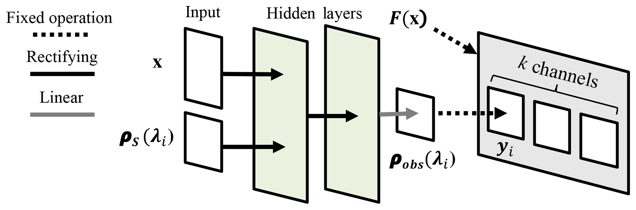
Figure 1Illustration of a single subnetwork in the neural RTM emulator. Each subnetwork predicts the top-of-atmosphere reflectance ρ_obs(λ_i) for a single channel centered at wavelength λ_i provided state parameters x and surface reflectance ρ_s(λ_i). Collecting the predictions generated by k subnetworks, each modeling distinct channels, and converting those predictions from ρ_obs to radiance emulates the RTM function F(x)→y for the selected channels.

Download

Constructing a robust neural RTM emulator from precomputed RTM outputs faces two fundamental modeling challenges. First, the precomputed RTM outputs must provide sufficient coverage of the state space to represent the distribution of spectral responses in each channel. Second, the subnetworks must accurately predict RTM outputs for intermediate state parameter values within the bounds of the state space for all channels. Intuitively, modeling channels whose spectral responses vary substantially with respect to small changes in state is more challenging than modeling more stable channels. For instance, small variations in the concentration of atmospheric water vapor can produce complex, nonlinear changes in spectral responses in the water absorption bands, while other wavelengths remain relatively unchanged. Accurately modeling unstable channels may require generating additional RTM outputs at increased sampling density to highlight distinct responses that are poorly represented in the existing precomputed outputs, and additional computational resources may be required to fine-tune the appropriate subnetworks to capture those distinctions.

To ensure each subnetwork reliably models its corresponding channel, we measure prediction accuracy on a test set of precalculated RTM outputs excluded from the training process. In our initial experiments, we used both traditional randomized cross-validation and bootstrap sampling to construct the training and test sets, but after we observed that the main sources of variability in the state space emerged from interactions among a small number of state parameter values, we concluded that randomized sampling of the state space without an informed sample stratification yields optimistic or inconsistent estimates of test accuracy and/or convergence time in cross-validation. Ultimately, we concluded that validation using a fixed and bounded subset of the state parameter values would provide a more informative assessment of model performance. Using a bounded subset also permitted direct comparison to lookup-table-based approaches, as they require upper and lower bounds on each variable to generate intermediate values via interpolation. We describe this approach in more detail later in this work.

We can also improve model accuracy and reduce computational demands by exploiting characteristics of the state space in tandem with RTM modeling assumptions. One means we use to achieve this is through a process of weight propagation. Rather than initializing the weights for each subnetwork from scratch, we use the converged weights of the subnetwork modeling the previous channel to initialize the weights for the subnetwork modeling the current channel, which are then fine-tuned to minimize the prediction error for that channel. Using weight propagation often yields a substantial reduction in training time in comparison to training each subnetwork from scratch, and can also improve prediction accuracy for channels whose RTM outputs are relatively stable with respect to the state space. An additional side benefit is that weight propagation provides an approximate means to account for channelwise coupling for instruments whose spectral response functions partially overlap for adjacent channels.

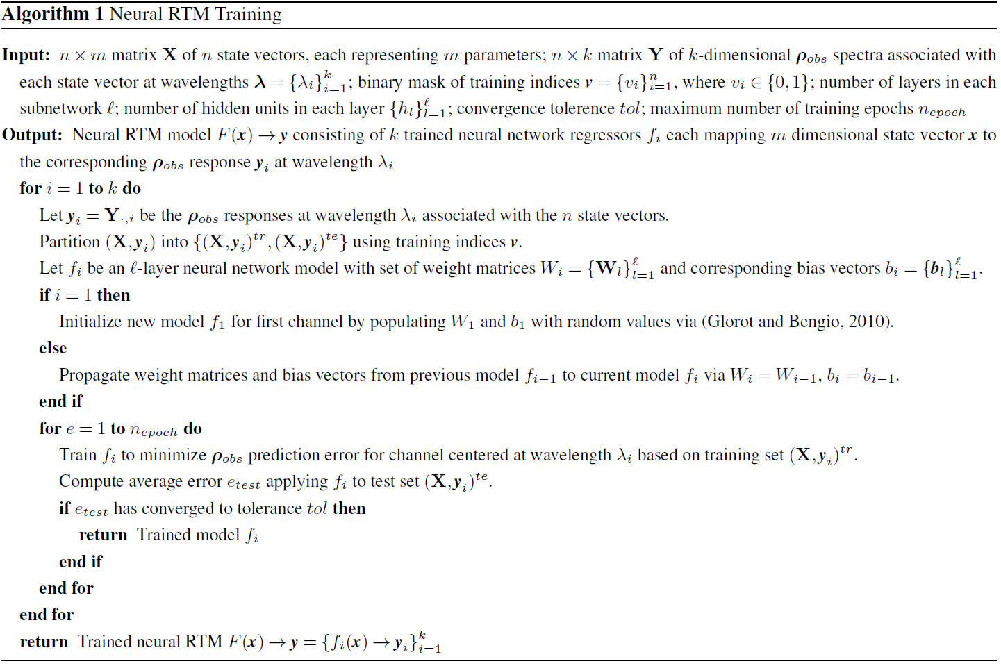
Algorithm 1 describes the procedure to train the neural RTM emulator provided n samples from the m-dimensional state space and their corresponding ρ_obs outputs, each spanning k channels. The output of the algorithm is a trained neural RTM that takes a state vector x of m parameters as input and outputs a k-dimensional prediction vector y, which we convert to radiance with respect to ϕ_o and e_o. The prediction vector is the concatenated output of the trained subnetworks $\mathit{\{}{f}_i{\mathit{\}}}_{i=\mathrm{1}}^k$ for each of the k channels.

Our goal is to train each subnetwork f_i to generate accurate predictions for states explicitly included in X and more importantly for intermediate states not explicitly included in X but within the bounds of the state space. To achieve this, we employ a sampling strategy that partitions the state space in a manner that helps to guide each subnetwork to accurately predict intermediate states. Specifically, we partition X and Y into disjoint training (X,Y)^tr and test (X,Y)^te sets such that X^tr contains all state vectors containing the boundary values {min(p_j),max(p_j)} of all state parameters. This partitioning ensures the training set contains the convex hull of the Euclidean subspace of ℝ^m defined by the state parameters and also that all test states in X^te represent intermediate states within the hull. To capture the internal structure of the state space within the hull, the training set should also contain one or more intermediate state vectors for each p_j satisfying $\min \left(p_j\right)<{\mathit{x}}_j^{\mathrm{tr}}<\max \left(p_j\right)$. Given the training and test partitions, we train each subnetwork to model the function f_i by minimizing the L²-regularized mean-squared error (MSE) between the predicted and the observed values of the n^tr training samples (X,y_i)^tr representing the ρ_obs responses for the ith channel.

Each subnetwork uses a feed-forward architecture with two hidden layers. The hidden layers use rectifying linear activation functions, which have been shown to be more robust than the sigmoid or tanh activations used in traditional neural networks (Nair and Hinton, 2010), and the output layer uses a linear activation function. We use the method proposed by Glorot and Bengio (2010) to initialize any subnetwork weights that are not initialized via weight propagation, and use the widely used error back propagation algorithm (Werbos, 1982) with adaptive moment estimation (Kingma and Ba, 2014) to optimize the weights via gradient descent. We train each subnetwork until we reach the maximum number of epochs n_epoch, stopping early if the mean absolute error (MAE) between the true and predicted outputs for each channel converges to within 0.1 %. This level of accuracy is sufficient to make the approximation error a smaller contributor to total uncertainty than other unknowns in the measurement system. For example, it is generally a similar magnitude to relative calibration error of different focal plane array elements, which can vary slightly due to drift between calibrations (Thompson et al., 2018a).

We define a case study to demonstrate the capabilities of our RTM emulator using data acquired by the PRISM imaging spectrometer (Mouroulis et al., 2008, 2014). PRISM uses a push-broom design and observes a cross-track angular field of view spanning approximately 30^∘, and is designed to observe coastal ocean environments in the 350–1050 nm spectral range at approximately 3 nm spectral sampling. The instrument was mounted onboard a high-altitude ER-2 aircraft which overflew Santa Monica, USA, in October 2015 at 20 km above sea level (Thompson et al., 2018b; Trinh et al., 2017). At this altitude, the instrument measured the scene through nearly all of Earth's atmospheric scattering and absorption, providing a challenging test case with relevance to future orbital instruments.

Table 1State parameters values used in libRadtran model runs to generate ρ_obs spectra to train and validate the neural RTM. State vectors containing the median value of each auxiliary parameter (indicated by bold text) are held out for testing, while the remaining state vectors are used for training the channelwise subnetworks.

Download Print Version | Download XLSX

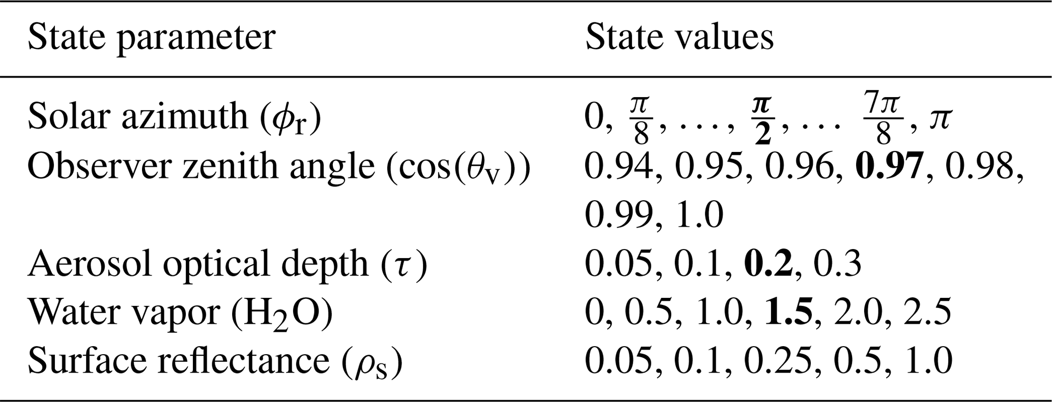
We consider a state space consisting of a single free parameter per instrument channel for the surface reflectance ρ_s, along with four m=4 state parameters that vary independently for every spectrum in a given flight line, which include the atmospheric aerosol optical depth at the surface, τ; the atmospheric water vapor content of the column in grams per square centimeter, H₂O; the cosine of the observer zenith angle, cos (θ_v); and the relative azimuth angle between the observer and the Sun, written ϕ_r. Each of these free parameters varies independently for every spectrum in a given flight line. Naturally, alternative parameterizations are possible, including mixture models, continuum-absorption models, and others. However, these could be mapped to our representation without loss of generality.

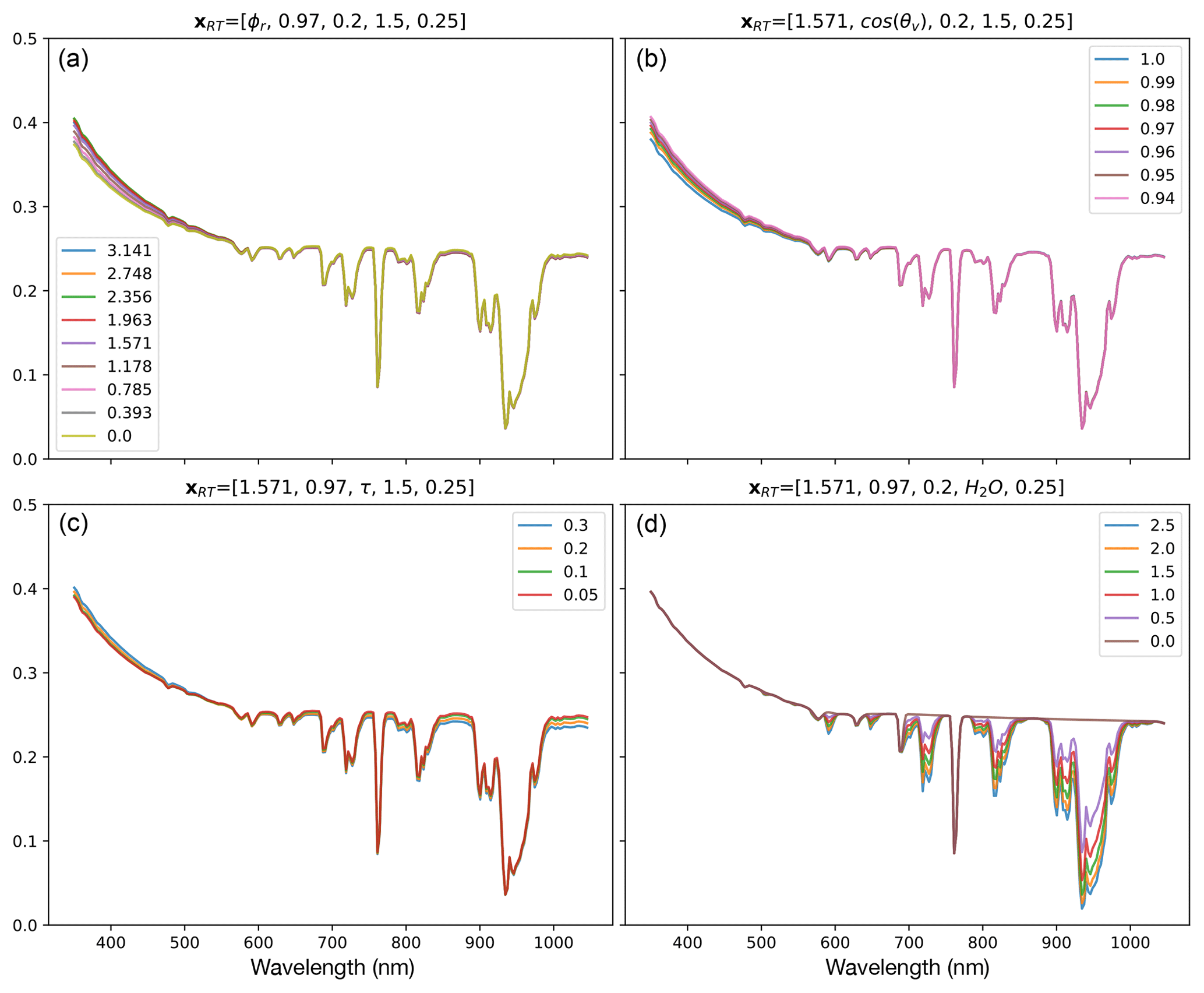
Figure 2ρ_obs spectra for ρ_s=0.25 spanning the range of the ϕ_r (a), cos (θ_v) (b), τ (c), and H₂O (d) parameters with respect to the validation grid values.

Download

We identified a set of values for each state parameter that covered the conditions anticipated during the flight campaign, and provided those values in Table 1. We generated RTM outputs using the libRadtran radiative transfer code (Emde et al., 2016; Mayer and Kylling, 2005) for a midlatitude summer atmosphere appropriate to the PRISM flight line we considered¹. Generating ρ_obs spectra for every combination of state parameter values yielded n=9072 total ρ_obs output spectra, each of k=7101 dimensions spanning the range of the PRISM instrument wavelengths with 0.1 nm spacing. Our test data consist of all state vectors containing the median value of each state parameter (shown in bold text in Table 1) and the ρ_obs spectra associated with those states. The remaining states and their corresponding ρ_obs spectra form our training set.

Figure 2 depicts the changes in the ρ_obs spectra with respect to parameters ϕ_r (panel a), cos (θ_v) (panel b), τ (panel c), and H₂O (panel d), while holding the other parameters fixed at their median values. Unsurprisingly, the most visibly dramatic changes occur as absorption features appear with increased H₂O vapor concentrations. Of the remaining parameters, only aerosol optical depth τ has an observable effect on spectral shape across the visible and near-infrared wavelengths. Changes induced by varying ϕ_r and θ_v are comparatively small and predominantly observable in the visible range.

For this case study, we focused on modeling F(x) based on libRadtran outputs resampled to the PRISM instrument channels. This dramatically reduced the computation required to construct the neural RTM, as we only needed to train a total of 245 subnetworks representing each of the PRISM channels with 2.83 nm spacing, rather than the 7101 channels at 0.1 nm spacing generated by libRadtran. We note that convolving the libRadtran spectra to the lower-resolution PRISM spectral response function (SRF) means the ρ_obs values are no longer strictly monochromatic. However, channelwise coupling is not a significant concern as the instrument channels are well-separated. In future work, we plan to construct a more general neural RTM that generates ρ_obs predictions at 0.1 nm spacing, can be subsequently convolved to the spectral response function associated with a particular sensor.

We observed experimentally that subnetworks consisting of two hidden layers with 50 units each and a training cycle of at most 500 epochs (where one epoch consists of a full pass of gradient updates over the training set) with batch sizes ranging from 100 to 200 training samples was sufficient for each subnetwork to converge to our error requirements for the state space parametrized by values in Table 1. Single-layer subnetworks were typically inadequate to model channels whose ρ_obs responses changed in a highly variable and/or nonlinear manner with respect to small changes in the state parameters (for instance, the water absorption bands). We set the initial learning rate to 0.001 with the following adaptive moment estimation parameters $\mathit{\{}{\mathit{\beta }}_{\mathrm{1}}=\mathrm{0.9},{\mathit{\beta }}_{\mathrm{2}}=\mathrm{0.999},\mathit{ϵ}={\mathrm{10}}^{-\mathrm{10}}\mathit{\}}$ and set the L² regularization penalty term α to 10⁻⁴ for each subnetwork. A longer training cycle or additional hidden units can be used to match the RTM output more precisely and would likely be necessary to model more complex state parameter spaces.

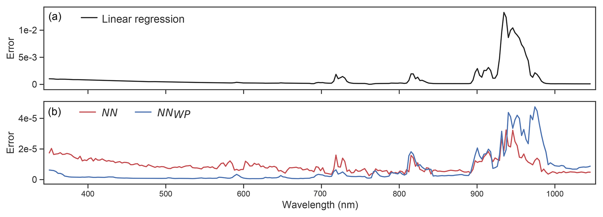
Figure 3(a) ρ_obs test prediction error per channel using channelwise linear regressors (black line). (b) Neural network test prediction error per channel using subnetworks trained from scratch (NN, red line) versus subnetworks trained with weight propagation (NN_WP, blue line).

Download

As a baseline comparison, we used the channelwise training samples ((X,y_i)^tr in Algorithm 1) to train a least-squares linear regressor on the ρ_obs responses for each channel, and applied each regressor to generate predictions on the associated test samples ((X,y_i)^te in Algorithm 1). The channelwise test errors of the linear regressors provide an upper bound on the piecewise, locally linear interpolation error incurred using lookup tables to infer ρ_obs responses for intermediate states. Figure 3 compares the ρ_obs test prediction error using the channelwise linear regressors (panel a, black line) to the error produced by the channelwise subnetworks trained from scratch (NN, blue line) versus channelwise subnetworks initialized with weight propagation (NN_WP, red line). The channelwise subnetworks yield an order of magnitude reduction in prediction error on all channels in comparison to the linear regressors, and demonstrates potentially significant issues with lookup-table-based approaches. Weight propagation provides an average reduction of 64 % in channelwise error, but also yields systematically higher errors in the H₂O absorption range between 890 and 1000 nm where the ρ_obs responses vary rapidly for adjacent channels.

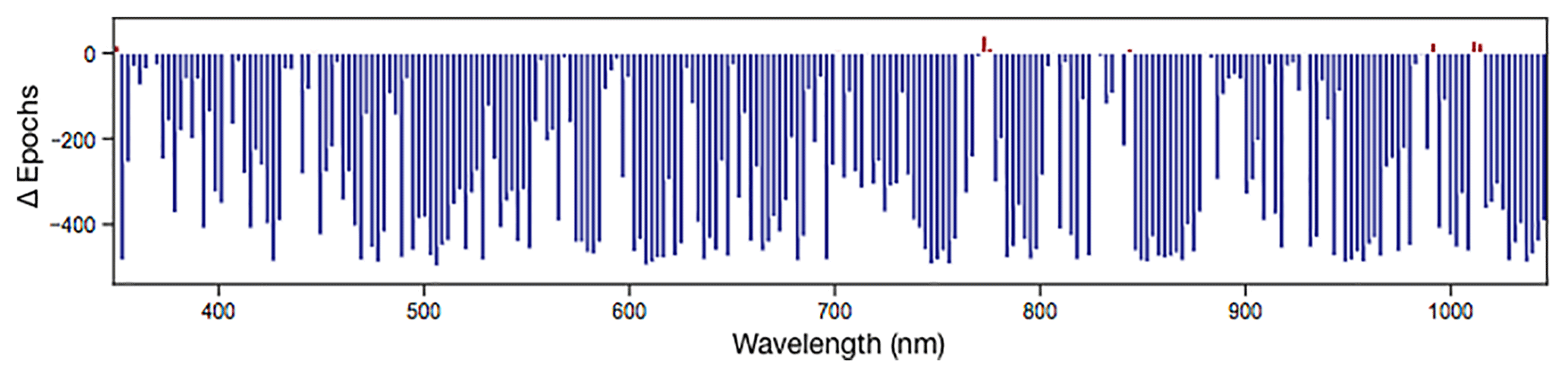
Figure 4Difference in training epochs to converge to 0.1 % validation error. Negative values (blue bars) show channelwise subnetworks that converged faster using weight propagation, while positive values (red bars) indicate channels whose subnetworks converged more quickly when trained from scratch.

Download

Figure 4 compares the number of epochs required to converge for channelwise subnetworks trained from scratch versus subnetworks initialized with weight propagation. Over the set of all PRISM instrument channels, weight propagation permits convergence in ≈70 % fewer epochs over subnetworks not leveraging weight propagation. In terms of raw compute time, our scikit-learn (Pedregosa et al., 2011) implementation requires 2–3 min to train a single monochromatic subnetwork from scratch on a single processor core, while subnetworks initialized with weight propagation typically require less than 30 s to converge. However, we note that the channelwise subnetworks trained with weight propagation converge as quickly in the 925–975 nm range – where their most significant prediction errors occur – as in the remaining channels. While it is unsurprising that the H₂O absorption wavelengths are challenging to model, the fact that the two weight initialization schemes yield distinct error distributions suggests that the subnetworks modeling those channels may not have converged.

Investigating further, we measured the average root-mean-square error (RMSE) on the test set with respect to the pairwise interactions between ρ_s and the four state parameters, and show the resulting error surfaces in Fig. 5. Relatively small errors for the majority of the parameter space indicate that the ρ_obs spectra vary smoothly with respect to most state parameter values, with the most significant variability emerging from a small range of values in the ${\mathit{\rho }}_{\mathrm{s}}\in [\mathrm{0.4},\mathrm{0.8}]$ and ${\mathrm{H}}_{\mathrm{2}}\mathrm{O}\in [\mathrm{1.0},\mathrm{2.0}]$ regions of the state space. The relatively high error in this regime is consistent with our earlier observation that small changes in the atmospheric water vapor parameter yield considerably different ρ_obs spectra, as shown in Fig. 2, and the comparatively high prediction errors for the H₂O absorption bands shown in Fig. 3.

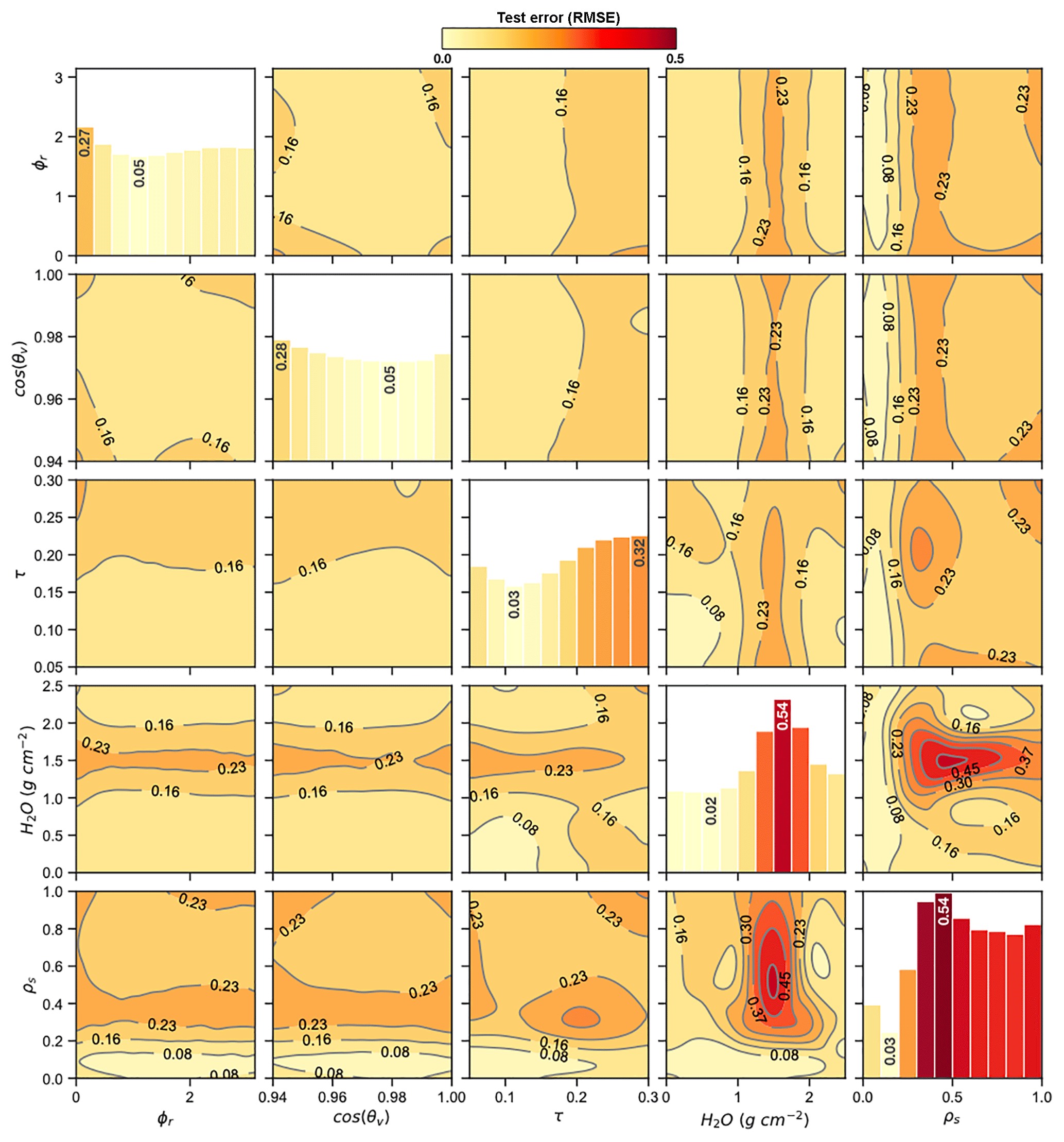
Figure 5Pairwise contour plots showing the ρ_obs test prediction error (RMSE) surfaces with respect to the state parameter values specified in Table 1. Contour labels on the off-diagonal subplots give the error levels associated with each contour. Diagonal subplots show the average RMSE in 10 uniformly spaced bins spanning the (x axis) range of each parameter. Vertical labels on the diagonal subplots indicate the minimum and maximum error values for each parameter and their corresponding bins.

Download

We now evaluate the neural RTM emulator in the context of a surface–atmosphere retrieval problem, retrieving surface reflectance for comparison to known surface materials. To that end, we fused the optimal estimation (OE) formalism of Rodgers (2000), following the specific approach of Thompson et al. (2018c) for application to imaging spectroscopy. The OE method estimates the atmosphere and surface state vector by an iterative least-squares optimization of the forward model's match to the measured radiances. Cost terms related to observation error and prior probabilities of state vector elements ensure rigorous propagation of uncertainties in the retrieval.

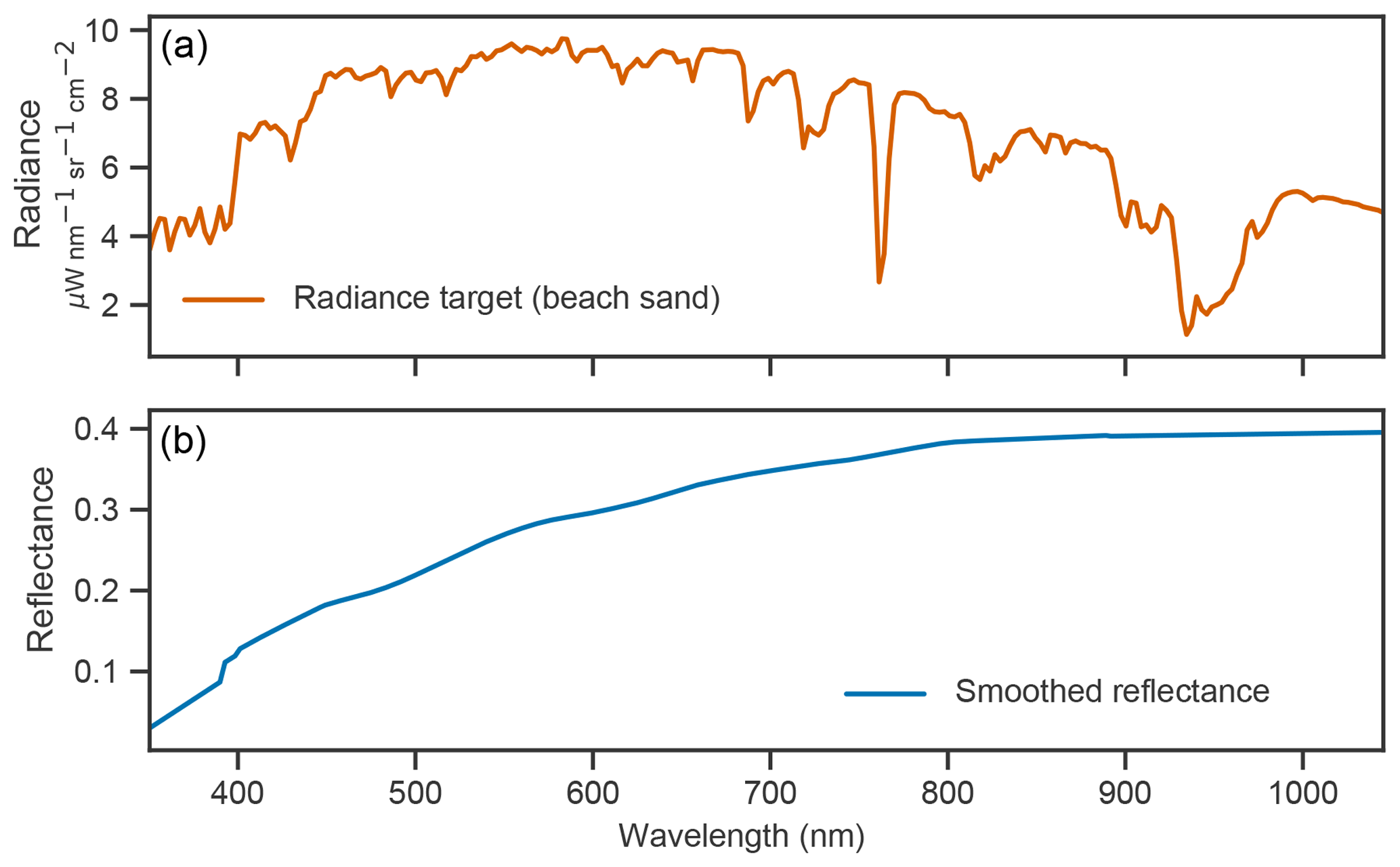
Figure 6PRISM radiance spectrum (a) and the resulting smoothed reflectance (b) spectrum for the beach sand target used in the vicarious calibration procedure.

Download

Continuing our case study, we begin by computing radiometric calibration factors for the PRISM flight line via vicarious calibration. This procedure, similar to standard practice calibration for imaging spectrometers (Thompson et al., 2018a), projects the residual error in retrieved surface reflectance back into radiance space where it becomes a multiplicative correction factor applied independently to each channel. We generate a “standardized” surface reflectance target by performing a first-principles retrieval for a beach sand radiance spectrum manually selected from the target PRISM image. We smooth the resulting surface reflectance spectrum to suppress significant atmospheric features, and use the smoothed spectrum to generate radiometric correction factors appropriate to our flight line. Applying the resulting factors fine tunes the calibration for optimal results and suppresses residual errors caused by uncertainty in spectral response or RTM inaccuracy. For reference, the beach sand radiance spectrum and the resulting smoothed surface reflectance spectrum are shown in Fig. 6.

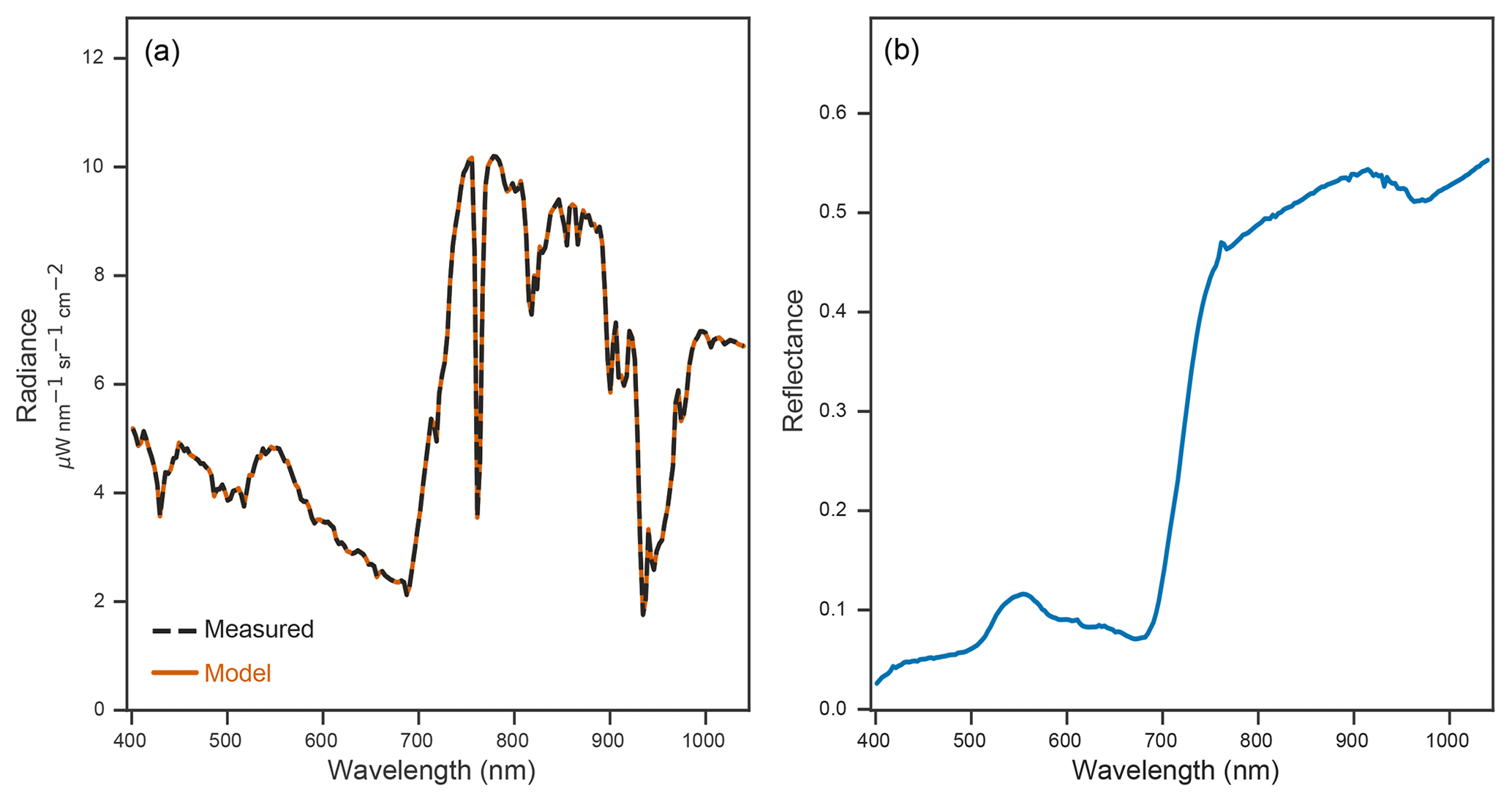
Figure 7Example surface reflectance retrieval for a PRISM vegetation spectrum. Panel (a) shows the measured (black dashed spectrum) versus predicted (orange spectrum) radiance spectra. Panel (b) shows the retrieved surface reflectance spectrum (blue spectrum).

Download

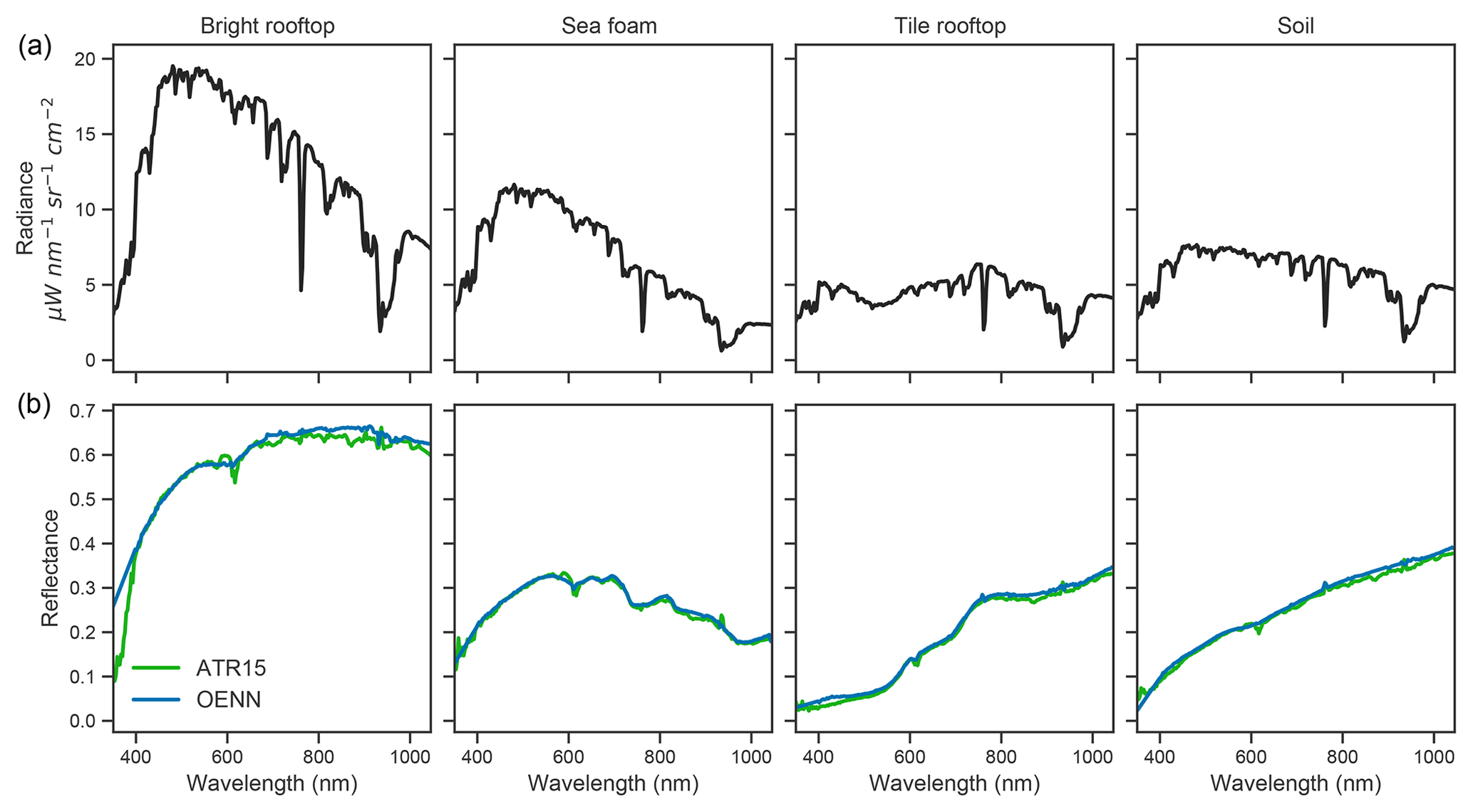
Figure 8Selected radiance spectra (a) and corresponding surface reflectance retrievals (b) using the ATREM-based atmospheric correction approach of Thompson et al. (2015) (ATR15, green spectra) versus optimal estimation equipped with our neural network RTM emulator as the forward model (OENN, blue spectra).

Download

We applied the atmospheric correction procedure to a set of radiance spectra from the PRISM flight line representing a diverse range of surface materials including grass, rooftop materials, soil, and seafoam. Figure 7 shows a successful retrieval result for a radiance spectrum representing grass on a golf course fairway. The inversion (orange line) perfectly matches the measured radiance (black dashed line) in Fig. 7a. In Fig. 7b, the estimated surface reflectance (blue line) is an extremely smooth and faithful estimate of a dark vegetation spectrum. Figure 8 shows additional radiance spectra (panel a) and their corresponding surface reflectance retrievals (panel b). The high-quality surface reflectance estimates – evidenced by the lack of residual bumps caused by atmospheric absorption and the flat, low surface reflectance profiles in the aerosol-dominated interval from 400 to 450 nm – provide additional confidence in the network's value for atmospheric correction. Our neural RTM emulator runs in less than 5 ms per PRISM spectrum (about 0.02 ms per channel). This represents a reduction of several orders of magnitude in runtime in comparison to analogous first-principles RTMs (i.e., monochromatic RTMs that solve the coupled scattering–absorption problem in a computationally exact manner, such as DISORT), which typically required over 10 min to generate a spectrum at 0.1 nm spacing (about 0.15 s per channel).

The Python source code used to train and apply the neural RTM for optimal-estimation-based atmospheric correction is available at https://github.com/dsmbgu8/isofit (last access: April 2019). The data used to train the RTM emulator, including the input state vectors and corresponding ρ_obs spectra resampled to PRISM instrument wavelengths, are also available in the examples/20151026_SantaMonica subdirectory at the above URL.

The supplement related to this article is available online at: https://doi.org/10.5194/amt-12-2567-2019-supplement.

Authors BDB and DRT conceived, implemented, and described the methodology and experiments described in this paper, and are the primary contributors to this work. SD contributed model analysis and RTM data collection during a Caltech Summer Undergraduate Research Fellowship (SURF) internship at JPL in summer 2017. ME and ROG provided expertise in the theory and application of imaging spectroscopy and atmospheric correction methods. VN provided expertise in radiative transfer modeling along with software and guidance for future efforts. TM contributed analysis and generated RTM outputs during a Caltech SURF internship at JPL in summer 2018. MP provided support and guidance for TM.

The authors declare that they have no conflict of interest.

This paper was edited by Lars Hoffmann and reviewed by two anonymous referees.