the Creative Commons Attribution 4.0 License.
the Creative Commons Attribution 4.0 License.
 | 07 May 2019
A segmentation algorithm for characterizing rise and fall segments in seasonal cycles: an application to XCO2 to estimate benchmarks and assess model bias
Leonardo Calle
Benjamin Poulter
Prabir K. Patra
There is more useful information in the time series of satellite-derived column-averaged carbon dioxide (XCO2) than is typically characterized. Often, the entire time series is treated at once without considering detailed features at shorter timescales, such as nonstationary changes in signal characteristics – amplitude, period and phase. In many instances, signals are visually and analytically differentiable from other portions in a time series. Each rise (increasing) and fall (decreasing) segment in the seasonal cycle is visually discernable in a graph of the time series. The rise and fall segments largely result from seasonal differences in terrestrial ecosystem production, which means that the segment's signal characteristics can be used to establish observational benchmarks because the signal characteristics are driven by similar underlying processes. We developed an analytical segmentation algorithm to characterize the rise and fall segments in XCO2 seasonal cycles. We present the algorithm for general application of the segmentation analysis and emphasize here that the segmentation analysis is more generally applicable to cyclic time series.
We demonstrate the utility of the algorithm with specific results related to the comparison between satellite- and model-derived XCO2 seasonal cycles (2009–2012) for large bioregions across the globe. We found a seasonal amplitude gradient of 0.74–0.77 ppm for every 10∘ of latitude in the satellite data, with similar gradients for rise and fall segments. This translates to a south–north seasonal amplitude gradient of 8 ppm for XCO2, about half the gradient in seasonal amplitude based on surface site in situ CO2 data (∼19 ppm). The latitudinal gradients in the period of the satellite-derived seasonal cycles were of opposing sign and magnitude (−9 d per 10∘ latitude for fall segments and 10 d per 10∘ latitude for rise segments) and suggest that a specific latitude (∼2∘ N) exists that defines an inversion point for the period asymmetry. Before (after) the point of asymmetry inversion, the periods of rise segments are lesser (greater) than the periods of fall segments; only a single model could reproduce this emergent pattern. The asymmetry in amplitude and the period between rise and fall segments introduces a novel pattern in seasonal cycle analyses, but, while we show these emergent patterns exist in the data, we are still breaking ground in applying the information for science applications. Maybe the most useful application is that the segmentation analysis allowed us to decompose the model biases into their correlated parts of biases in amplitude, period and phase independently for rise and fall segments. We offer an extended discussion on how such information about model biases and the emergent patterns in satellite-derived seasonal cycles can be used to guide future inquiry and model development.
- Article
(3415 KB) -
Supplement
(2029 KB) - BibTeX
- EndNote


Most of our understanding about atmospheric CO2 dynamics has come from CO2 sampled by in situ flask samples or eddy flux towers on the Earth's surface (Ciais et al., 2014). While these data streams have proved incredibly useful, the transient dynamics of fluxes simulated by global-scale terrestrial models have only been compared to relatively few locations on Earth. In contrast to surface CO2 samples, which sample CO2 concentrations in the planetary boundary layer, satellite observations of CO2 are made by downward-looking Fourier spectrometers from the top of the atmosphere and represent an integrated estimate of CO2 concentrations in a full column of atmosphere, hereafter “XCO2” (Wunch et al., 2011; Crisp et al., 2012). Although fluxes from the surface have a large influence on the total column CO2, the vertical and horizontal transport of air masses in higher atmospheric layers, each with different concentrations of CO2, also influence the CO2 concentrations in the total column (Belikov et al., 2017), including that of the stratosphere (Saito et al., 2012).
The synoptic coverage and integrated nature of XCO2 means that surface fluxes from around the globe impart information into the seasonal dynamics and interannual variability of regional seasonal cycles, which is both a confounding and useful property for evaluating large-scale models. The integrated nature of the data also means that even a few years of data will be sufficient to evaluate the simulated dynamics of global-scale models. We propose that if models can reasonably simulate the timing and magnitude of terrestrial surface fluxes in all bioregions, then we would expect that the simulated XCO2 would match reasonably well with the seasonal dynamics from the benchmark satellite data. Such demonstrated ability could strengthen confidence in regional-to-global model simulations.
To gain insight into seasonal cycle dynamics of satellite XCO2 and individual model behavior, we demonstrate a novel approach to extract more information from the seasonal cycle than is typically characterized. In evaluations of model performance, traditional performance statistics (root-mean-square error, correlation, standard deviation) are used to quantify bias in phase and amplitude of the seasonal cycle against a benchmark signal (Coupled Model Intercomparison Project Earth system models in Glecker et al., 2008; Dynamic Global Vegetation Models, DGVMs, in Anav et al., 2015). In almost all applications, however, the entire time series is treated at once without considering detailed features at shorter timescales, such as nonstationary changes in amplitude, magnitude, period or phase (Fig. 1). We suggest that traditional performance statistics be applied to categories of unique patterns in the seasonal cycle and not to the entire time series, thereby characterizing the error structure in a manner that can relate temporal dynamics (amplitude, magnitude, phase) with unique underlying processes.

Figure 1Conceptual diagram for the segmentation analysis. (a) Interannual variation in seasonal cycle amplitudes (vertical, solid colored lines) and periods (horizontal, dashed colored lines); such interannual variation may also differ among rise and fall segments. (b) A reference cycle (black) and a modeled seasonal cycle (red) are compared using the root-mean-square error (RMSE), which is taken as the difference in magnitude at the same exact time in reference and modeled seasonal cycles. In out-of-phase signals, the RMSE misrepresents bias. The segmentation approach matches segments in the reference and modeled seasonal cycles, rise to rise and fall to fall, so that the errors in magnitude and phase can be decomposed and directly represented (c).
We extend and apply a time series segmentation method (Ehret and Zehe, 2011) to extract the rise and fall segments in seasonal cycles of satellite-derived and simulated XCO2, based on a suite of terrestrial ecosystem models. The advantage of the segmentation approach is that it allows an error structure to be accurately characterized by separately calculating the errors in amplitude, period and phase for each segment type (rise, fall). For example, in a graph of a multiyear seasonal cycle of XCO2 (Fig. 1), each increasing and decreasing segment is visually discernable and analytically differentiable from other portions in the seasonal cycle; hereafter, rise refers to increasing segments and fall refers to decreasing segments in a seasonal cycle. The rise and fall segments largely result from seasonal differences in the onset and cessation of terrestrial ecosystem production (Keeling et al., 1995), which means that a segment's signal characteristics (i.e., amplitude, period, phase) are likewise influenced by different stages of terrestrial ecosystem activity. By segmenting the time series into similar component signals, we can then test for differences in the signal characteristics of rise and fall patterns and provide insight into a model's ability to recreate these features of the seasonal cycle over multiple years.
Our first aim was to simply characterize the satellite-derived XCO2 seasonal cycles in terms of rise- and fall-type segment variation. Secondly, we evaluated if signal characteristics and model biases differed or were correlated among rise and fall segments, which would help provide information in the missing parts of the satellite-based time series (i.e., at high latitudes during boreal winter and in the tropics during the wet season), which we demonstrate is possible. We also evaluated if model biases between rise and fall segments differed enough to provide information about the underlying model representation of terrestrial dynamics, which we underscore as possible, but discuss the limits for inference in this regard. Lastly, we explored how a single modeled process (land use and land cover change, LUC) manifests in the different signal characteristics and biases in rise and fall segments. We offer discussion on how the segment-based model biases and emergent patterns in satellite-derived seasonal cycles can be used to guide future inquiry and model development.
2.1 Satellite XCO2 data
Satellite observations of XCO2 were obtained from the Greenhouse gases Observing SATellite (GOSAT; v.7.3). Onboard the satellite, a Fourier Transform spectrometer measures the thermal and near-infrared absorption spectra of the constituent atmospheric gases within the footprint of observation (∼10 km). Satellite data were freely obtained and analyzed only for 2009–2012 because they corresponded to the overlapping timeframe of available simulation data. The data were downloaded from NASA Goddard Earth Sciences (GES) Data and Information Services Center (DISC) online repository (https://oco2.gesdisc.eosdis.nasa.gov/data/GOSAT_TANSO_Level2/ACOS_L2_Lite_FP.7.3/; last access: 25 April 2018). We used the Level 2 Lite data products, which include only high-quality and bias-adjusted data points, based on the Atmospheric CO2 Observations from Space (ACOS) retrieval algorithm v.7.3 (Crisp et al., 2012; O'Dell et al., 2012).
Note that satellite data have uncertainties of their own based on instrument noise, the version of retrieval algorithm used to filter atmospheric effects and averaging kernels (Yoshida et al., 2011; Lindqvist et al., 2015). We made the assumption that averaging kernels have a minimal effect on extracted seasonal cycles, and we did not apply the averaging kernels to the simulation data in this study. A full quantification of uncertainty in satellite-derived seasonal cycles is beyond the scope of this study, but such an analysis could be useful for benchmarking purposes, as models continue to reduce large biases (≫1.0 ppm). Nevertheless, we make the assumption that lower biases are generally indicative of better model performance.
2.2 Simulated terrestrial fluxes from DGVMs
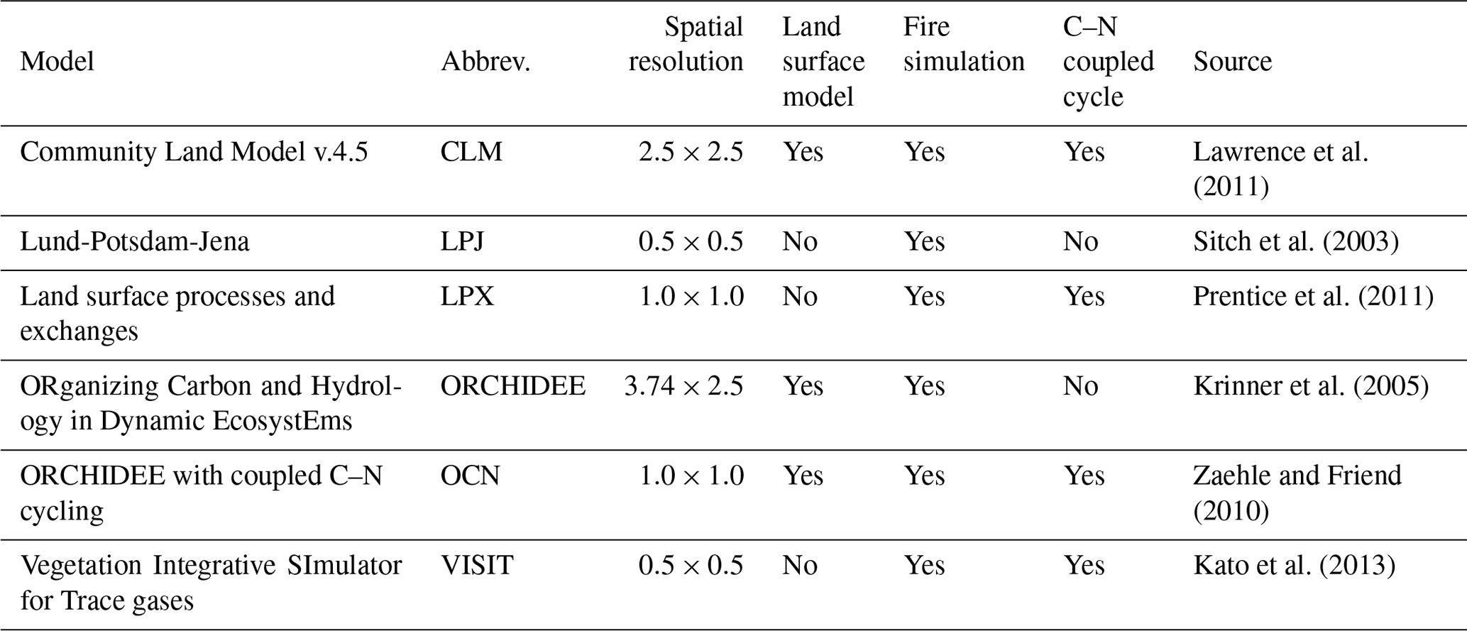
The net biome exchange (NBP) from the land to the atmosphere was simulated by six terrestrial ecosystem models (Table 1) that were part of the TRENDY model intercomparison project v.2 (Sitch et al., 2015, http://dgvm.ceh.ac.uk/, last access: 24 April 2019). We use the atmospheric convention and make fluxes to the atmosphere positive and fluxes to the land negative. We assumed that the primary modes of seasonal variability in terrestrial NBP at large scales are described by three terms: net ecosystem production (net primary production and heterotrophic respiration), fluxes from fire and land use change (LUC). The protocol for the DGVM intercomparison standardized the (i) forcing data – gridded (0.5∘) climate data (air temperature, short- and long-wave radiation, cloud cover, relative humidity, and precipitation) and global annual mean CO2 – and the (ii) initial conditions for time-varying simulations for the past century (1860–2012). We used simulated NBP for two sets of model simulations, one where land use (natural vegetation, crop and pasture fractional cover) is fixed at values from the year 1860 (“S2” scenario described in Sitch et al., 2015) and another where land use change is simulated according to the HistorY Database of the global Environment (HYDE v3.1; Goldewijk et al., 2011) (“S3” scenario as described in Sitch et al., 2015); both simulation types were forced with time-varying climate and CO2.
Table 1Terrestrial ecosystem models from the TRENDY v.2 model intercomparison used to simulate terrestrial net ecosystem exchange. All models simulate carbon (C) cycles, whereas some models also include nitrogen (N) cycles, identified as C–N coupled models.
2.3 Fossil fuel and ocean fluxes
The modes of variability (trend, seasonality, intra-annual and interannual variability) in XCO2 are also influenced by fluxes from oceanic exchange, fossil fuel consumption and cement production. We used a simplified model of oceanic CO2 exchanges from Takahashi et al. (2009) and monthly mean fossil fuel emissions from the European Commission's Emissions Database for Global Atmospheric Research (EDGAR v.4.2) based on country-level reporting and emissions factors and the Fossil Fuel Data Assimilation System (http://edgar.jrc.ec.europa.eu/, last access: 24 April 2019).
2.4 Simulated XCO2 using an atmospheric model
Simulations of atmospheric CO2 were conducted for the period of 2009–2012 using the land, ocean and fossil fuel fluxes. We used the Center for Climate Systems Research/National Institute for Environmental Studies/Frontier Research Center for Global Change (CCSR/NIES/FRCGC) chemistry transport model (ACTM) based on an atmospheric general circulation model (Patra et al., 2009). The ACTM was run at a horizontal resolution of T106 () and 32 sigma-pressure vertical levels. The simulated XCO2 values were obtained by taking the sum of the pressure-weighted CO2 concentrations over all vertical layers, equivalent to the column-averaged observations. We then used “collocation” sampling of the ACTM XCO2 data to match the location and timeframe (13:00 local time) of observations: ±5 d to account for sub-weekly transport errors (i.e., by averaging; Guerlet et al., 2013). We obtained the simulated XCO2 for each component flux (land, fossil fuel, ocean) and finally summed the components to get the XCO2 used in bias evaluations.
2.5 Extraction of XCO2 seasonal cycles
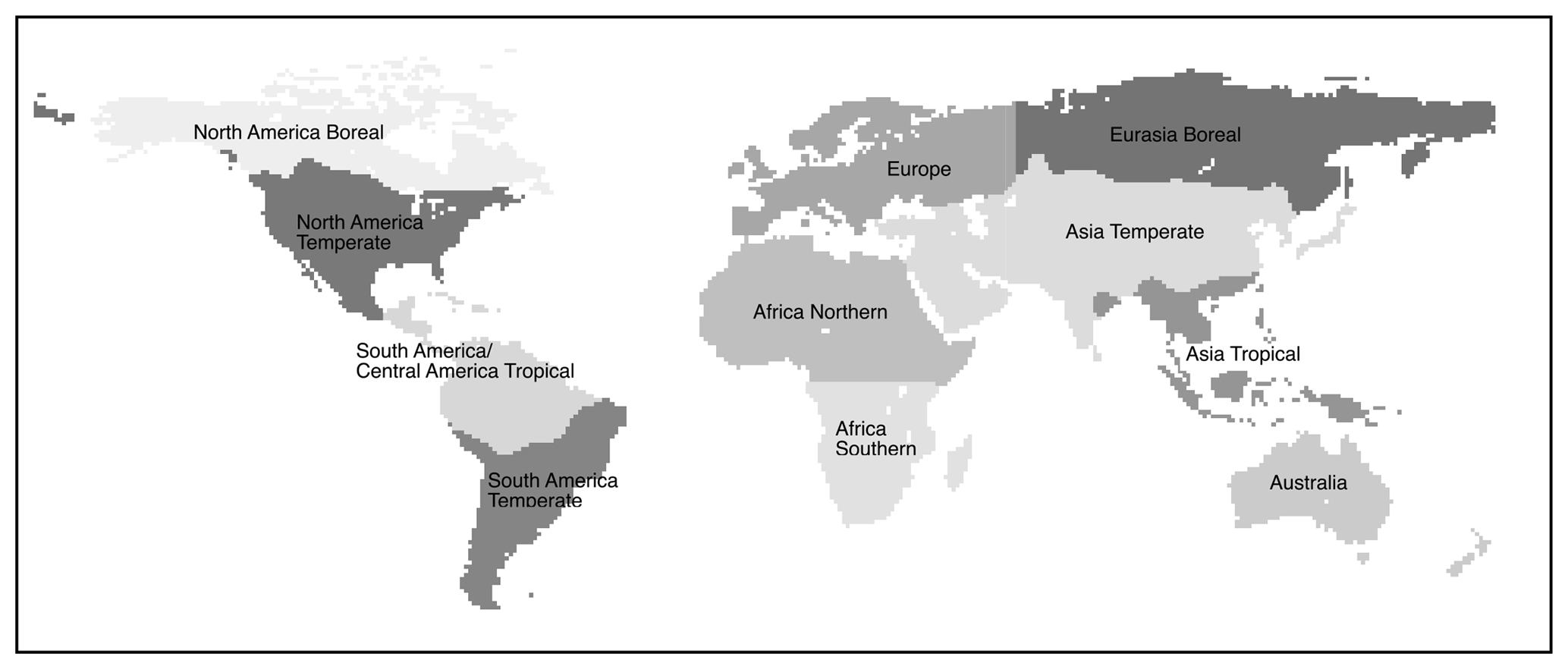
We first estimated the mean of daily XCO2 values by averaging gridded values within each of the 11 TransCom regions (Fig. 2) for both the observed and modeled XCO2. This procedure was as straightforward as written above, and the accompanying computer code (software: R) is provided in the Supplement. We then applied a digital filtering algorithm (ccgcrv, by Thoning et al., 1989; https://www.esrl.noaa.gov/gmd/ccgg/mbl/crvfit/crvfit.html, last access: 24 April 2019) to the mean time series to extract the long-term trends and seasonal cycles, fitted as a two-term polynomial (linear growth rate was used because the time series spanned only 3 years) and a four-term harmonic function to account to seasonal asymmetry. Temporal data gaps were linearly interpolated by the algorithm. After subtracting the long-term trend and seasonal cycle, the ccgcrv algorithm filters the residuals in the frequency domain using a Fast Fourier Transform (FFT) algorithm to retain short- and long-term interannual variation (additional details in Nakazawa et al., 1997; Pickers and Manning, 2015). The cutoff for the short-term filter was set at the recommended value of 80 d (Thoning et al., 1989). The short-term cutoff of 80 d retains data variations that are evident or maintained for the timescale of 3–4 months (4.56 cycles yr−1). The cutoff for the long-term filter was set to a large number (3000), which is longer than the number of days in our time series (365 d yr−1 × 3 years = 1095 d) because, with such a short time series, we needed to force the estimation of a linear trend with no interannual variation; otherwise, the algorithm would be too sensitive and derive variation in the trend without practical justification. For all analyses in the following, we combined the seasonal cycle with the digitally filtered short-term variation and used the derived data points along the smoothed seasonal cycle curves for analysis.
2.6 Technical description of algorithm: segmentation of seasonal cycles
The purpose of this section is to describe the technical algorithms used in the analysis. These algorithms are based on concepts put forth by Ehret and Zehe (2011), translated herein into the R computing language (R Development Core Team, 2008). Where Ehret and Zehe (2011) focused on single hydrological events, we modify and restructure the algorithm to accommodate much longer nonstationary cyclic time series for general application to seasonal cycle analyses. An R package for the segmentation algorithm is freely available at the GitHub repository (https://github.com/lcalle/segmentTS, last access: 24 April 2019) . A permanent version of the code is available in the Dryad Digital Repository (https://doi.org/10.5061/dryad.vk8ms62). The computer code is annotated and provides data used in this study with demonstrations for applying the algorithm to remove local minima or maxima and the categorization of seasonal cycle segments.
2.6.1 Categorizing segments and isolating seasonal rise and fall cycles
We first determine the first derivatives numerically. The ccgcrv signal decomposition algorithm outputs a daily time series in the form of a multidimensional array, but we focus on a subset of the array – the two-dimensional rectangular matrix representing points along the detrended seasonal cycle:
where the first column is the row index, the second column is made up of dates, the third column is the detrended XCO2 ppm with the short-term variation added back in and the rows are the triplets of the index: time in the x direction and magnitude (XCO2 ppm) in the y direction.
We can numerically determine the first derivative in the y direction at each point via differencing:
We then classify each row in first column () into one of the following categories below and expand B to an n×4 matrix to store the classified values. The main objective is to classify the endpoints (trough, peak) of the rise and fall segments:
We then take the subset of endpoints (S) in the classified matrix B,
where S retains the dimensions of the B. A unique segment (s) is defined as a set of two consecutive endpoints (rows) in S that alternate in their classification of trough or peak, meeting the following condition:
We identify local minima and maxima that are deviations in otherwise longer (seasonal) and more general rise and fall patterns based on two criteria below, and then reclassify the segments based on the class of the segment with the largest amplitude. The amplitude of a segment (as) is defined as follows:
where s1,2 is the first endpoint in the second column (XCO2 ppm), either a trough or a peak, and s2,2 is the second endpoint for the specific segment, where, by definition, the first endpoint must be classified (s1,4) as one of peaks or troughs and must not have the same classification as the second endpoint (s2,4).
The first criterion sets a minimum threshold for the amplitudes, redefining the set of endpoints defining the segments as follows:
Segments that represent local minima or maxima that are not of interest to the user can be identified through a comparison of amplitudes of consecutive segments, dropping the segment with the lowest amplitude as follows:
This procedure results in a new subset of segment endpoints with consecutive elements that have a similar classification (e.g., ), which needs to be rectified. We keep the endpoints with the lowest trough value and the largest peak value:
where s[t] is a unique segment in the set of s segments, s[t+1] is the following consecutive segment, and are the segment first and last endpoints, respectively, and s[t]* is the updated segment with new endpoints and , while segments s[t] and s[t+1] have been removed from the set of segments (s).
A (subjective) limit can also be set to exclude or include segments based on temporal proximity. For example, consecutive minima (minima–maxima–minima) should not be considered local minima if separated by 365 d; these are probably real local minima driven by processes unique to different seasons. By contrast, local minima separated by 60 d may represent signals within the overall seasonal rise and fall pattern (e.g., due to fire). For this study, we are more interested in assessing the general seasonal patterns. We therefore estimate the temporal distance, in “days” (Ds), between the first endpoints of consecutive segments and evaluate the condition as follows:
where is the endpoint date in the x direction, and the minimum threshold for distance between endpoints is set at a conservative 250 d (∼8 months), ensuring that only the main rise and fall patterns within a given year are captured. This conditional evaluation also results in a new subset of segments (s*) with consecutive elements that have a similar classification, as above, but Eq. (9) can be reapplied to select the endpoints, which represent general rise and fall patterns.
Additional criteria can be applied to automate the removal of local minima and maxima that are not relevant to the user, but we caution that visual inspection of the signal is important to avoid unwanted reclassification of segments in the time series.
2.6.2 Human-assisted pattern recognition via visual inspection
The procedure outline in Sect. 2.6.1 is applied to both the reference (R) and modeled (M) seasonal cycle time series. In the best of cases, the procedure would result in matrices for R and M, each with an equal number of segments and the same sequence of endpoint classes (trough–peak–trough–peak, etc.). In practice, however, the number and sequence of segments in M will not always equal the number or sequence of segments in R. When variability in the modeled seasonal cycle results in many local minima (maxima), and therefore many short rise (fall) segments, there can be a mismatch between the indices of segments, wherein smaller and shorter segments in M are matched to much larger and longer segments in R; this is simply an artifact from the automation of the procedure outlined previously. Although we have implemented automated procedures in the algorithm that reconcile these types of mismatches, we found that it was considerably quicker to (i) conduct a “blind” run of the algorithm on the data, (ii) visually inspect the automated graphical plots of the seasonal cycles for mismatching segments (Fig. S1 in the Supplement), (iii) identify the index of the mismatching endpoints in M and then finally (iv) rerun the algorithm specifying the index of the endpoint in M for removal.
2.6.3 Segment signal characteristics and error statistics
The amplitude (Eq. 6) and period (p in days) for all segments are first characterized, with the period defined as follows:
where sn and s0 are the end and start dates of a segment, respectively. Then, for each segment in M and R, a complementary vector Mx and Rx is created in the x direction with a fixed number of equally spaced dates,
Each element in Mx corresponds, by index, to an element in Rx, such that a matching pair exists. Similarly, the complementary vectors My and Ry are created in the y direction, with the length of the vector matching the length of the vector in the x direction (k). For each element in My and Ry, we perform a linear interpolation of the values of XCO2 ppm in B () for the indices given by the dates in Mx and Rx; fortunately, the linear interpolation is automated by the approx function in R, which makes this procedural step straightforward. The end result is, for every segment in M and R, four vectors of equal length in Mx, My and Rx, Ry, with the timing of the data and values of XCO2 ppm that follow the corresponding seasonal cycles in B. We can then decompose the corresponding errors in phase and magnitude along the time series.
Although in this paper we focus only on errors in amplitude, period and phasing of the segments, the time series of errors in timing and magnitude are an additional level of detail in the error structure that is evaluated by the segmentation algorithm.
2.7 Statistical summaries
For each of the rise and fall segments within a region, we summarized the characteristics by averaging the amplitude (ppm), period (days) and phase, which we estimated in two ways based on the day of year for the first and last endpoint of the corresponding segment (DOY start, DOY end, respectively). For model biases, we used the total sum of the component tracers (land and fossil fuel and ocean) and we summarized model biases as the region average of segment-to-segment differences between model and observation. Although we aggregate the biases among segment types, and therefore lose information, we do this to demonstrate that there are distinct general patterns in the rise and fall segments, regardless of region. Of course, one might be more interested in one bioregion over another, and while this is indeed possible and suggested, such analysis is not the intent of this paper.
The latitudinal variation in amplitude and period length for rise and fall segments was evaluated by comparing the regionally averaged metrics against the average latitude of each TransCom region. We sought to evaluate a model's ability to reproduce the north to south gradient in seasonal cycle characteristics. We also use data from in situ CO2 flask samples for 2005–2015 (NOAA/ESRL/GMD CCGG cooperative air sampling network; https://www.esrl.noaa.gov/gmd/ccgg/flask.php, last access: 1 May 2018) as a check for evaluating latitudinal variations in surface site seasonal amplitudes. Surface sites were selected if they had a minimum of 5 years of data between 2005 and 2015, with at least one flask sample per month. The peak–trough amplitude was then taken from monthly averaged data. Linear correlations were deemed statistically significant at levels of p=0.05.
The amplitude and period length asymmetries between rise and fall segments were calculated as in the following example. Given a sequence of data with segments of type {Fall_1, Rise_1, Fall_2, Rise_2}, representing seasonal cycles over 2 years, three asymmetries in amplitude and period length would be calculated for the sequence of segments, as (i) Fall_1 − Rise_1, (ii) Fall_2 − Rise_1 and (iii) Fall_2 − Rise_2. The asymmetries are referenced to fall segments such that, for example, negative asymmetries mean that the amplitude (or period length) is greater in the rise segment. The reason we calculated asymmetries between segments immediately before and after the fall segments is because we assumed that there is some degree of autocorrelation in the relational values that is both real and could provide useful information, but the underlying causal mechanisms are speculative at this point.
2.8 Application of approach
We applied the approach to evaluate the effect of LUC on XCO2 by using the segment characteristics setting the S2 scenario as the reference time series and then following procedures outlined in Sect. 2.6 to match corresponding rise and fall segments in the S3 and S2 simulations. We then calculated the difference in the amplitude, period and phase between matching segments, hereafter defined as the “LUC effect”. To evaluate the relative influence of the LUC effect on changes in amplitude, period and phase, we transformed the LUC effect to percentages by (a) dividing the LUC effect in amplitude by region-specific average amplitudes and (b) dividing the LUC effect in the period length and phase (DOY start, DOY end) by the region-specific average period lengths. We then pooled the absolute values of the standardized LUC effects for all regions by model; the absolute values of the LUC effect were used because we were more interested in any significant change, rather than a directional change in the metric values. We conducted an analysis of variance to test for significant differences among models and types of LUC effects (amplitude, period and phase), in terms of the percent LUC effect, also setting significant differences at p=0.05. In this manner, we were able to determine the relative importance of the LUC effect by these metrics and compare amongst the models.
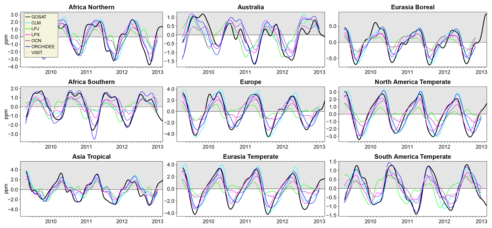
Figure 3Detrended XCO2 seasonal cycles by TransCom region. Simulated seasonal cycles are the sum of transported fluxes from DGVM, fossil fuel and ocean, but only the DGVM model name is listed.
3.1 Satellite coverage and XCO2 seasonal cycles
The satellite data coverage had sufficient temporal density to extract smooth seasonal cycles (Fig. 3), except during boreal winter at high latitudes (>50∘ N) and during the wet season in tropical Asia, where there was clear evidence of linear interpolation over large data gaps (Figs. S2–S4). We had to exclude North America Boreal and South America Tropical regions from all analyses because the data were too sparse and seasonal cycles could not be derived. The mean number of satellite retrievals per day in 5∘ bins was greater than 1 when averaged over a season, but the spatial distribution of the retrievals by month (Figs. S2–S4) showed that only portions of the TransCom regions were being represented with satellite observations. The lack of a complete representative sample of satellite observations in a region suggests that the derived seasonal cycle will be biased towards the XCO2 observations in those subregions with greater coverage. We take this finding as a caveat but also demonstrate below that the derived seasonal cycles are a good representation of the general seasonal dynamics in the data.
There were noticeable deviations (local minimums) from otherwise consistent rise and fall patterns during a season (for example in North Africa in Fig. 3). We compared the seasonal cycles derived from DGVM XCO2 collocated with GOSAT retrievals against DGVM seasonal cycles using all simulated XCO2 and complete coverage (no collocation). For the single DGVM studied in this side analysis, the local deviations were still evident in the seasonal cycles that used data with complete coverage (Fig. S5). We believe that these deviations are not artifacts of the spatial distribution of satellite retrievals but instead are true patterns in the XCO2 seasonal cycle. However, the collocation sampling did appear to have a greater effect on the amplitudes and periods in Southern Hemisphere regions, whereas the effect of collocation sampling was less influential in Northern Hemisphere regions.
The magnitude of the GOSAT seasonal cycle residual error, averaged over all regions, was 0.15±1.02 ppm, which was not a small fraction relative to the average amplitudes when taking into account the standard deviation. However, the residuals were normally and randomly distributed around zero (Fig. S6), which we took to suggest that there was no systematic bias, that the daily spatial variation in data coverage averaged out and that what we derived was a realistic estimate of seasonal variation in XCO2.
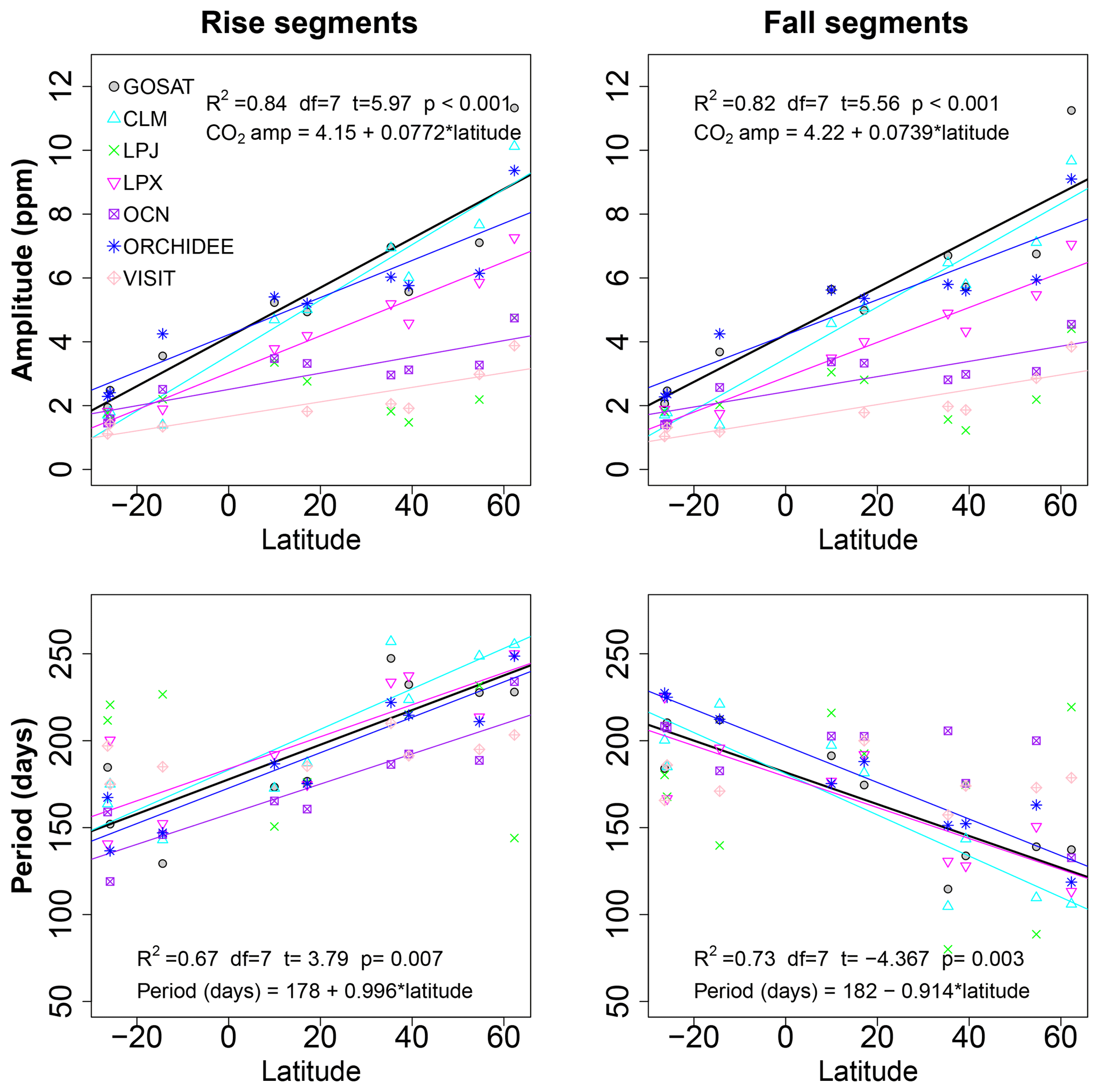
Figure 4Latitudinal variation in amplitude and period in rise and fall segments among TransCom regions, using the average latitude for each region. Linear regressions are shown when significant (p<0.05). Regression statistics and equation are only given for GOSAT.
3.2 Latitudinal variation in XCO2 seasonal cycle amplitudes
Seasonal amplitude varied predictably with latitude (Fig. 4). Latitude explained between 82 % and 84 % of the variation in seasonal amplitudes in GOSAT, with the range taken from linear models of rise and fall segments (Fig. 4). There was an increase in amplitude of 0.74±0.13 ppm (μ ± SE, standard error) for rise segments and 0.77±0.13 ppm for fall segments for every 10∘ latitude for GOSAT. Whereas the XCO2 amplitudes exhibited a linear relationship with latitude, in situ flask samples of CO2 exhibited a log-linear relationship with latitude (Fig. 5; R2=0.90, df = 45, p<0.001), which indicates larger amplitude gradients at higher latitudes than at lower latitudes. The difference results in a latitudinal range (Equator to 70∘ N) in seasonal amplitude of ∼7 ppm for XCO2 (taken as ], as the largest possible amplitude gradient in XCO2; SE) and ∼17 ppm for surface CO2. The dampened gradient in XCO2 amplitude suggests substantial north–south atmospheric mixing, which is consistent with a previous study on the meridional vs. zonal contribution to XCO2 via atmospheric transport (Keppel-Aleks et al., 2012). In addition, the in situ sampling stations are located in such a way that they sample the “background” atmosphere, which reduces the influence of local to regional terrestrial fluxes, and instead they provide seasonal cycles representative of hemispheric and continental scales. The contrast between the latitudinal gradient in amplitude between XCO2 in this study and in situ surface samples may therefore be even greater than reported here (Olsen and Randerson, 2004; Sweeney et al., 2015).
Only LPX was able to simulate the GOSAT-derived latitudinal gradient (slope) in amplitude, but, even in this model, the magnitudes of the amplitudes were consistently lower than GOSAT by ∼1.5 ppm (Fig. 4). ORCHIDEE simulated the latitudinal gradient in amplitude reasonably well and CLM simulated a marginally stronger north–south gradient, whereas the gradient was much weaker in two models (OCN, VISIT) and there was no statistically detectable amplitude gradient in LPJ. The evidently enhanced meridional mixing of total column CO2 complicates an interpretation of the finding that most models simulated a weaker gradient in XCO2 seasonal amplitude (Fig. 4). It makes it difficult to determine why models do not reproduce the latitudinal gradient in amplitude very well. For example, are the magnitudes of the fluxes in certain regions too low or too high, such that they offset the seasonal amplitudes in the region of interest after atmospheric transport? We offer suggestions in the Discussion that might help answer these questions.

Figure 5Latitudinal variation in the amplitude for detrended in situ surface CO2 samples. Data are the average of peak–trough amplitudes for 2005–2015, only including sites with a minimum of 5 years of data. Points are labeled according to the three-letter code of the sampling station. The South Pole (spo), Mauna Loa (mlo) and Barrow Island (brw) sites are highlighted in red for reference, as they are commonly referenced in literature. The latitudinal range in surface site CO2 seasonal amplitudes (∼19 ppm) is more than 2 times the latitudinal range in seasonal amplitudes of XCO2.
3.3 Latitudinal variation in XCO2 seasonal cycle period
The period lengths of GOSAT XCO2 seasonal cycles also varied predictably with latitude (Fig. 5), and there was no significant difference in the magnitude of the latitudinal gradients between rise and fall segments, although the direction of the gradient was positive for rise segments and negative for fall segments (Fig. 4). Latitude explained between 67 % and 73 % of the latitudinal variation in period lengths of GOSAT seasonal cycles. From south to north, the period lengths of rise segments increased by 10 d per 10∘ latitude for GOSAT. From south to north, the period lengths of fall segments had negative gradient and decreased by −9 d per 10∘ latitude for GOSAT. The opposite gradient in the period lengths of rise and fall segments implies that around 2∘ N the periods of rise and fall segments are of equal duration. North of this point of inversion in asymmetry, the period lengths of rise segments are greater than in fall segments, with an increasing asymmetry as latitude increases. We hypothesize that the latitude at the point of inversion of period asymmetry is a characteristic indicator of global atmospheric dynamics and biosphere productivity. Our rationale is that if (i) the primary driver of the period of drawdown (fall) or release (rise) in XCO2 seasonal cycles is the terrestrial biosphere, and (ii) DGVMs themselves simulate the terrestrial biosphere, then variation in the simulated point of inversion of asymmetry by different DGVMs suggests a strong influence of biosphere activity on this emergent pattern. The most obvious driver affecting the period is plant phenology. Furthermore, we already know that seasonal cycle in XCO2 is dominated by flux seasonality in land biosphere, while ocean and fossil fuel emission seasonality plays only a secondary role. Nevertheless, a north or south shift in the latitude of inversion (i.e., 2∘ N) would indicate that long-range transport of atmospheric signals, such as the poleward transport of southerly signals (Parazoo et al., 2016), has changed substantially. In which case, the relative contribution of long-range signals from southerly locations to seasonal cycle anomalies (in phase or amplitude) in northerly locations might be greater or lesser than expected. As of yet, however, it is unclear if this point of inversion is relatively stable over time or if, instead, the point shifts in latitude among years or decades depending on the relative influence of source–sink dynamics in biospheres in the Northern Hemisphere and Southern Hemisphere.
Most models correctly simulated the satellite-derived latitudinal gradient in the period, but LPJ and VISIT did not simulate statistically significant gradients in either rise or fall segments, and LPX could only reproduce the gradient for rise segments but not for fall segments (Fig. 4). For CLM, OCN and ORCHIDEE, the simulated gradients were statistically similar to GOSAT, although the absolute period lengths differed by up to 25 d. The latitudinal gradient in the period of XCO2 seasonal cycles is emergent from the underlying timing and duration of biosphere productivity, and, as such, it serves as a high-level constraint on simulated dynamics. It may therefore be possible to add this emergent pattern as a benchmark to evaluate models that attempt to reproduce more direct indicators of biosphere activity, such as seasonal patterns in leaf area (Richardson et al., 2012) or primary production (Forkel et al., 2014).
Table 2Signal characteristics for rise and fall segments of the GOSAT-derived XCO2 seasonal cycles (2009–2012) by TransCom region. The timeframe of one rise plus one fall segment approximately equates to 1 year. North America Boreal and South America Tropical regions were excluded for lacking the observations required to derive signals for rise or fall segments.
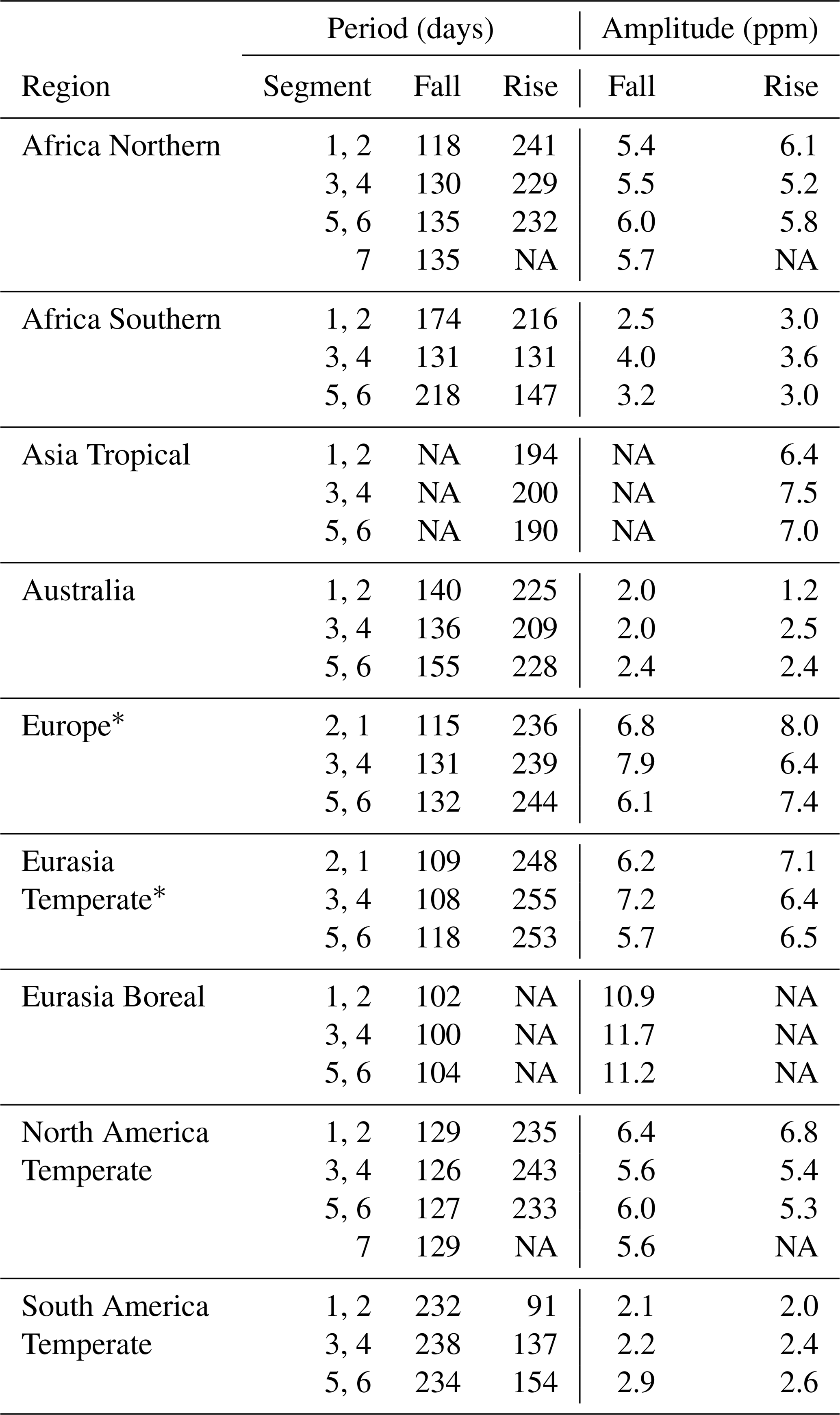
* The first differentiable segment is a rise segment, starting approximately d after the first segment in other regions because the initial drawdown (fall segment) in the region is a partial or incomplete segment. NA indicates that data are not available.

Figure 6Period asymmetries (a) and amplitude asymmetries (b) in GOSAT XCO2 seasonal cycles. The bars represent differences in amplitude or period for consecutive fall (F) and rise (R) segments, taking the fall segment as reference. For example, if the time series follows the sequence F1, R1, F2, R2, F3, R3 (i.e., three seasonal cycles), then the difference between the first segment (F1) and the second segment (R2) is calculated as “F1–R2”; a zero value would indicate that the metrics (amplitude or period) were equal, whereas an asymmetry would be indicated by a positive (F1 > R2) or negative (F1 < R2) value. By definition, consecutive segments cannot be categorized as F–F or R–R. Asymmetry statistics are not traditional summaries, but, nevertheless, they are characteristic and, in some regions, persistent patterns of the seasonal cycle that are undoubtedly influenced by biosphere activity.
3.4 GOSAT asymmetries in period and amplitude
The period asymmetry between rise and fall segments (Table 2) is clearer when comparing the periods of consecutive rise and fall segments (Fig. 6), taking the fall segment as reference, as described in Sect. 2.7. The period asymmetries were in the same direction except for the Africa Northern, Africa Southern and South America Temperate regions (Fig. 6a). The asymmetries exhibit stable patterns of consistent direction within many regions, and they also display quite a bit of interannual variation in the magnitude (or direction in some cases) of the asymmetries themselves (Fig. 6a and b). For example, the standard deviation in period asymmetry averaged 11 % of the region-averaged periods for GOSAT seasonal cycles, and it was greatest for the Africa Southern region (42 %). For context, a 10 % change amounts to a change in period asymmetry of 5–29 d and as much as 73 d in the Africa Southern regions, which is certainly a remarkable change in the atmospheric signal. The period asymmetries can provide insight into the underlying terrestrial dynamics, for example, from interannual variation in the duration of the carbon uptake period (Xia et al., 2015; Fu et al., 2017), but it is yet unclear how changes in carbon uptake period manifest to affect these patterns of asymmetry. Furthermore, one DGVM (ORCHIDEE) was able to simulate period asymmetries, consistent in direction, with that of the GOSAT record when using collocation sampling. However, the magnitude of the period asymmetry for ORCHIDEE was about half that of GOSAT, but it does suggest that the surface fluxes from this DGVM were more realistic in timing and magnitude. All other models had greater interannual variation in the direction of the asymmetry, with no other model reproducing the direction of asymmetry in all regions.
The amplitude asymmetries between consecutive rise and fall segments were more variable in the direction of the asymmetry for GOSAT (Fig. 6b). There was no consistent pattern in the direction or magnitude of the amplitude asymmetries within or among regions, but we did not investigate if there were annual patterns that were consistent among all regions. No model successfully reproduced the direction of asymmetry in amplitude across all regions in all years. As of yet, the relevance of interannual variation in the asymmetries is speculative, but we do know that such variation is not simply due to data coverage (Fig. S5) so there may be more insightful information in the signal.
3.5 Correlated biases between rise and fall segments
The correlations of model biases differed more between the Northern Hemisphere and Southern Hemisphere (NH and SH, respectively) than among regions, so we present the following analyses not by region but by NH and SH. The NH regions were comprised of Africa Northern, Europe, Eurasia Temperate, North America Temperate; the SH regions were comprised of Africa Southern, Australia and South America Temperate. These analyses required data on both rise and fall segments, which eliminated the Asia Tropical and Eurasia Boreal regions from these analyses.
Among rise and fall segments and among all models and regions, the model biases in amplitude were nearly perfectly correlated (NH, R2=0.99, df = 28, t=64.63, p<0.001; SH, R2=0.99, df = 16, t=65.02, p<0.001; Fig. 7a and e). Other than ORCHIDEE and CLM, which exhibited the smallest amplitude biases, the other models all had amplitudes that were too low. In the SH, there was a similar pattern of negative amplitude biases (Fig. 7e), with the exception of CLM, which simulated amplitudes that were too large in two of three SH regions. The strong correlations suggest that knowing the amplitude biases in one part of the seasonal cycle is sufficient to gain information about amplitudes in the missing part of the seasonal cycle. This might be particularly useful for constraining estimates of XCO2 seasonal cycle patterns during timeframes that have poor satellite coverage (boreal winter, tropical wet season). Furthermore, it is revealing that models, which simulate amplitudes that are too low, do so almost equally for both rise and fall segments, which is suggestive of a systematic bias in the sensitivity of the models to seasonal changes in climate. Such systematic biases can be due to simulated fluxes that are overall lower in magnitude or due to a pattern of spatiotemporal fluxes that end up offsetting or canceling each other in the atmospheric domain, but we cannot definitively attribute the bias of individual models to one of these possible causes yet.
The average period biases of rise and fall segments were also strongly correlated, with a greater strength of correlation in the NH (R2=0.77, df = 22, , p<0.001) than in the SH (R2=0.82, df = 21, , p<0.001). In the NH, almost all models simulated periods that were too short in rise segments and too long in fall segments in approximately equal and opposing amounts (Fig. 7b). In the SH, the period biases spanned both positive and negative values for both of the fall and rise segments but also in approximately equal and opposing amounts of bias (Fig. 7f). There were only a few data points where the periods within a region were either biased (i) too short for rise segments and also too short for fall segments or (ii) where the rise segment was biased too long and the fall segment was also biased too long. These patterns are suggestive of underlying constraints that compensate for biases in periods, such that situation (i) and (ii) rarely occur. Such constraints are likely associated with the underlying drivers of the period of rise and fall segments. For instance, models that simulate growing seasons that are too long will likely simulate fall segment periods that are also too long, and, as a consequence, the dormant season will be shortened, as will the periods of associated rise segments. Within a given model, the magnitude of compensating biases varied by region, so it is possible that biases in biosphere activity varied similarly by region. To incorporate such insights will require direct manipulation of the phenology represented by models, but improving the emergent patterns in the period to better match the satellite-derived XCO2 seasonal cycles will bolster confidence in the model's ability to represent both fine-scale dynamics and the emergent large-scale atmospheric patterns.
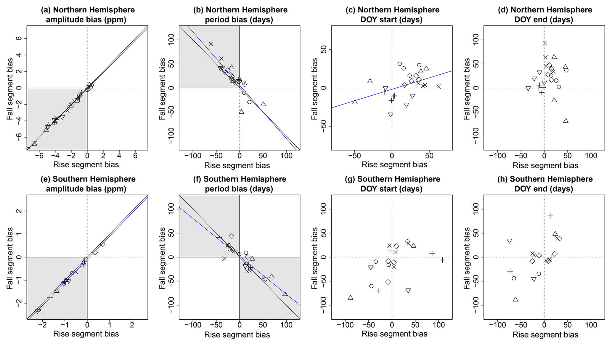
Figure 7Emergent correlations among biases for rise (x axes) and fall (y axes) segment model biases, using GOSAT XCO2 as a reference, for TransCom regions in the Northern Hemisphere (a–d) and Southern Hemisphere (e–h). Data points are the average bias by model (unique symbols, not shown) for a particular region. Data for the Eurasia Boreal and Asia Tropical regions were excluded for lack of data in both rise and fall segments. Diagonal black lines are the 1 : 1 correspondence lines; blue lines are significant linear correlations.
3.6 Application of approach: LUC effects on amplitude, period and phase metrics were nontrivial
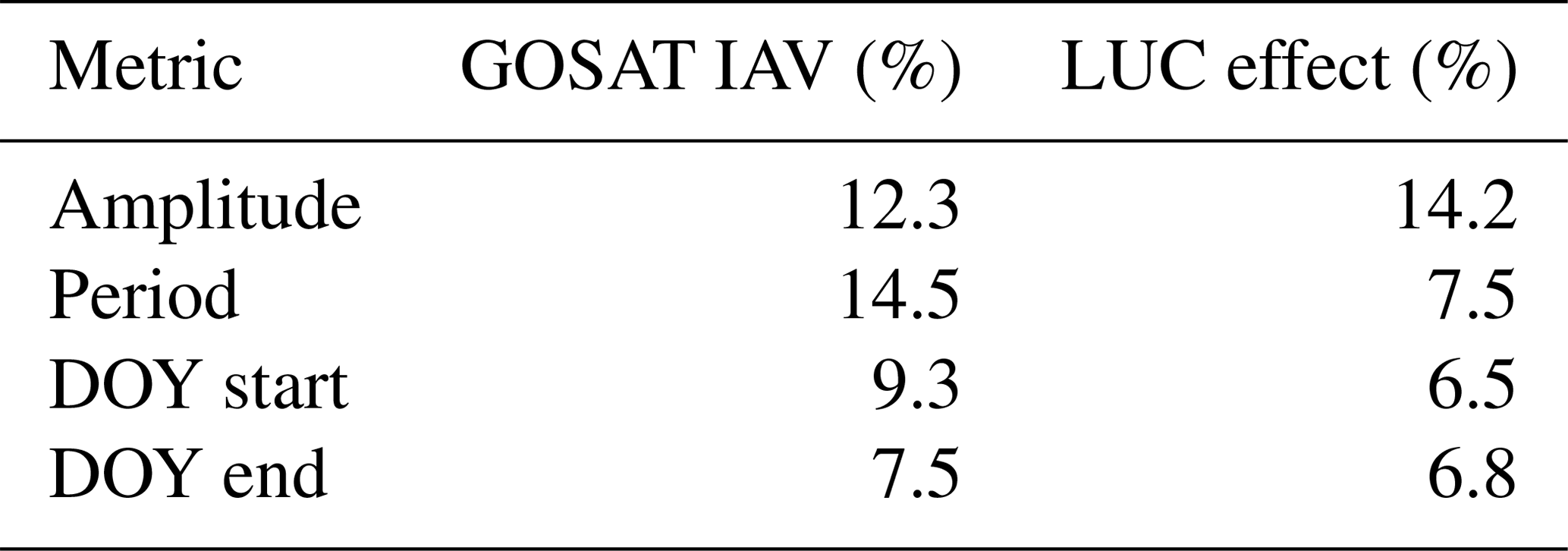
We describe the LUC effect as the percent change in the rise and fall segment amplitude, period and phase (DOY start, DOY end) when LUC processes are included in model simulations, relative to seasonal cycle metrics when LUC was not included in simulations. Among all models and rise and fall segments, the average LUC effect was largest on amplitude (mean 13.4 % or 0.37 ppm), but there were also nontrivial changes in the period (7.2 % or 13.2 d) and phase metrics of the DOY end (6.5 % or 11.4 d) and DOY start (6.2 % or 11.4 d). An analysis of variance suggested that the LUC effects did not significantly differ between rise and fall segments (F=0.006, df = 1, p=0.941), the specific model explained 16% of the variation (F=15.183, df = 5, p<0.001), and the metric explained only 5 % of the variation (F=7.815, df = 3, p<0.001). LPJ was an outlier in that it simulated larger LUC effects in every metric (mean LUC effect = 18 %), approximately 8 % greater than other models. The remaining variation in LUC effect was explained by the larger LUC effect on amplitude in LPX and VISIT (Fig. 8), whereas OCN simulated only marginally greater LUC effects than CLM and ORCHIDEE. The LUC effects were of similar magnitudes to the baseline interannual variation for these metrics, in terms of percent change, or greater in the case of the LUC effect on amplitude (Table 3).
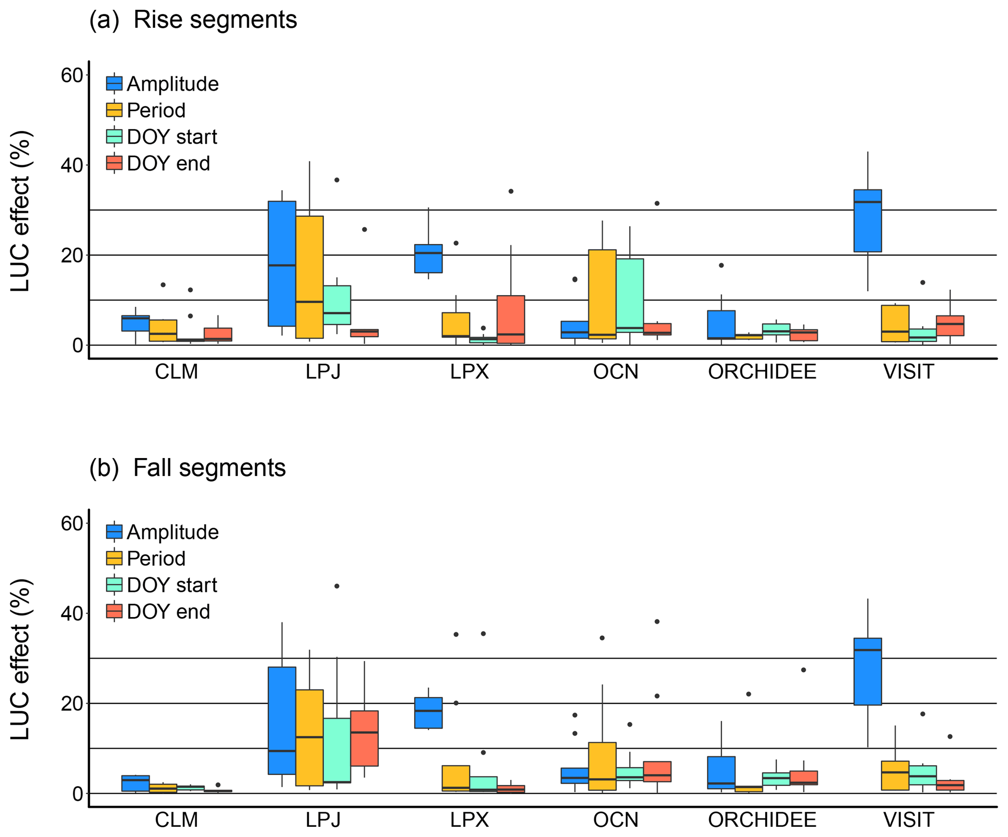
Figure 8Land use change effect on amplitude, period and day of year (DOY). The percentages were calculated from the difference in the metrics between simulations (S3–S2), scaled relative to amplitude and period of rise and fall segments for each region and model. DOY was scaled against the period.
The importance of the LUC effect on the amplitude of rise and fall segments was somewhat expected because LUC directly affects the type of land cover simulated in the models, for example by converting forest to pasture or pasture to forest and thereby influencing the magnitude of surface fluxes directly (Arneth et al., 2017). However, the effect of LUC on the temporal metrics of the seasonal cycle (period, phase) is typically understated in the literature. The LUC effects on period and phase are of the same relative magnitude as is observed in 2 decades of advancement in the start and end dates of the carbon uptake period, based on atmospheric inversion studies (Fu et al., 2017). It should not be a surprise then that LUC can affect the timing of surface fluxes, but this facet is often overlooked when the focus is solely on variability on annual or decadal timescales. At the very least, this work shows that land surface modelers should consider the impact of LUC on the timing and duration of surface fluxes, in addition to its effect on the magnitude of the fluxes.
Table 3The interannual variation (IAV) in XCO2 seasonal cycle metrics, presented as the relative standard deviation (i.e., RSD or coefficient of variation) and the LUC effect, defined as the change in the XCO2 seasonal cycle metrics when land use change is included in simulations, relative to simulations with only natural vegetation. The values for IAV and the LUC effect presented below are first calculated for each region and segment type (rise, fall) and then averaged over all regions and models (for the LUC effect). The values for the phasing metrics (day of year, DOY) are calculated using the period as the divisor.
4.1 Utility of a segment analysis for analyzing cyclic time series
We demonstrated that a segmentation analysis of satellite-derived XCO2 seasonal cycles can generate direct estimates of amplitude, period and phase at global and hemispheric scales. In addition, it can reveal stable patterns in the metrics, which can be used as benchmarks to evaluate simulation models. There is obvious value in using standard statistics (RMSE, SD, R2, etc.) to characterize a time series and evaluate it against simulated reproductions (e.g., “Taylor diagrams”; Taylor, 2001; Fig. S7). We do this too, but we argue that applying statistical measures of goodness of fit over the entire time series misses an opportunity to extract valuable information from observational data and provide more direct measures of bias. Studies that have evaluated amplitude and period biases directly have been based on the mean harmonic of the seasonal cycle (Peng et al., 2015), which lacks interannual variation, and therefore does not fully represent the modeled biases. Furthermore, the metrics for the asymmetric rise and fall patterns in seasonal cycles are not typically estimated or evaluated for bias. In the Europe region, for example, the interannual variation in amplitude (1.25 ppm) and period (25 d) is certainly not trivial (Fig. S8) and if excluded in evaluations it would cause a biased assessment of what the models can and cannot do well, limiting the potential of such assessments to inform potential improvements.
Our study focused on the rise and fall segments in XCO2 seasonal cycles, corresponding to periods when terrestrial ecosystems generally release and uptake carbon dioxide, respectively. Other studies might be more interested in shorter-term, pulse-type signals, such as the ability of models to simulate the effect of large-scale fires or volcano eruptions in an atmospheric time series. In either case, the segmentation algorithm could help standardize and decompose model bias into its component parts of amplitude, period and phase biases.
4.2 Asymmetries provide new insights into the interannual variation in atmospheric signals
By definition, the asymmetries (Fig. 6) are not anomalies, but, similarly, the amplitude asymmetries are directly related to underlying processes generating the imbalance in the amplitude and period between rise and fall segments. Most likely, the asymmetries reflect the difference in the magnitude or in the timing of fluxes during the growing season for fall segments and phenological dormancy for rise segments (Randerson et al., 1997). Whereas the signature of the terrestrial biosphere may be a more dominant driver of the period asymmetries, the amplitude asymmetries may also be influenced by processes that the models simply do not simulate well – or in any sufficient manner in some cases – such as sub-seasonal representation of fire and LUC (Earles et al., 2012) or volcano eruptions (Jones and Cox, 2001). The interannual variation in XCO2 period and amplitude asymmetries are directly related the activity of terrestrial ecosystems, but questions remain – are the annual asymmetries in amplitudes or periods evidence of a global response to large-scale climate phenomena, such as the El Niño–Southern Oscillation? Do some regions dominate and influence the signal more than others? To what degree do the asymmetries in one region provide information about asymmetries in other regions, and can we infer dynamics in Boreal regions, for example, by analyzing atmospheric signals in regions where satellite coverage is more complete? The asymmetries offer a new level of information on atmospheric dynamics that is ripe for exploring.
4.3 The effect of LUC on seasonal cycles is in addition to the effect on the long-term trend
Much focus has been put on accurately characterizing component fluxes from land use and land cover change simulated by DGVMs (Pongratz et al., 2014; Calle et al., 2016), but we also show that LUC influences the atmospheric seasonal cycle period and phase at a level that is comparable to the reference rates of interannual variation in those metrics (Table 3). This underscores the complex problem of trying to simultaneously resolve the contribution of LUC fluxes to the long-term trend in atmospheric CO2 (Le Quéré et al., 2018) and also to represent realistic LUC effects on seasonal-scale biosphere activity (Betts et al., 2013; Bagley et al., 2014). For instance, when land is converted from forest to pasture, the dominant land cover will affect the duration and timing of the surface fluxes (Fleischer et al., 2016) and this seems obvious. However, DGVMs were not developed during the era of satellite XCO2 observations, and thus the main issue of trying to resolve the effect of large-scale changes in land use for both the long-term trend and seasonal cycle dynamics is not easily solved. But now that these data are available, perhaps a new approach is necessary to take advantage of these large-scale benchmarks.
The inclusion of LUC in the simulations, after including the contribution from fossil fuels and ocean, resulted in a combined long-term trend estimate that was too large, by 0.07 to 1.72 ppm yr−1, compared to the long-term trend of GOSAT XCO2 (2.16±0.01 ppm yr−1) (Fig. S9). The GOSAT estimate is comparable to an independent estimate of the long-term trend of XCO2 from SCIAMACHY for the 2000s (1.95±0.05 ppm yr−1; Schneising et al., 2014). If we assume that this study's simulated long-term trends of fossil fuel fluxes (4.44±0.008 ppm yr−1) and those of the ocean ( ppm yr−1) are better constrained than the trends from the land fluxes, then according to the GOSAT benchmark, the simulated land sink is too weak. Despite the possibility that these simulated LUC fluxes are too high, the DGVM versions applied in this study do not simulate a suite of land management processes (shifting cultivation, wood harvesting, pasture harvest, agriculture management) that have been shown to increase the annual LUC flux by 20 %–60 % (Arneth et al., 2017), further pointing to a simulated land sink that is too weak. DGVM-based estimates of the terrestrial land sink have been compared against a residual term in the global carbon budget that is taken as the average flux over a decade (Le Quéré et al., 2018), but perhaps we are overlooking something here. The cumulative fluxes simulated by the models in this study (from 2002 to 2012) resulted in a long-term trend that is at odds with the satellite record, and it is unclear why. We must therefore attempt to reconcile biases in both the long-term trend and seasonal cycle dynamics if we are to use XCO2 or other integrated atmospheric measurements to constrain model dynamics and not simply assess these patterns independently.
4.4 Caveats, limitations and ways forward
The XCO2 gradient in amplitude is approximately half the gradient in amplitude of in situ surface CO2. The dampened XCO2 gradient suggests the presence of strong meridional mixing, which complicates accurate attribution of model biases to any specific bioregion. In effect, the XCO2 seasonal cycle is comprised of the fluxes from all regions to varying degrees (Olsen and Randerson, 2004; Sweeney et al., 2015; Lan et al., 2017). Given this, simulating the atmospheric transport of the surface fluxes from all regions at once would allow us to both (i) obtain useable estimates of model bias and (ii) to provide attribution to those biases. Indeed, the model biases were fully described but only in terms of XCO2, not in terms of terrestrial surface fluxes themselves. An approach for attribution of model bias in XCO2 might be laid out similar to Liptak et al. (2017), wherein the surface fluxes from each region (by year) undergo independent atmospheric transport. In a framework similar to this study, such simulations might prove instrumental in determining the fractional contribution of each region's fluxes to XCO2 seasonal cycle characteristics while also providing better guidance for model development.
Model evaluations also showed that few models have low bias in all seasonal cycle metrics of amplitude, period and phasing of simulated XCO2. An inherent requirement for reproducing the XCO2 signal is that the land-to-atmosphere fluxes are reasonable in magnitude, duration and timing in all land regions or, at the very least, in land regions with large vegetative areas that might disproportionately dominate the signal. Even though such requirements may be necessary to simulate the amplitude asymmetries, this is an extreme level of proficiency that the models simply do not currently exhibit.
Lastly, the relative contribution of land, ocean and fossil fuel fluxes to the seasonal cycle differs by region, latitude and time period (Randerson et al., 1997). This poses some concerns because fossil fuel and cement fluxes are considered to have low uncertainty, but they may be biased too high in some regions (Saeki and Patra, 2017), affecting our interpretation of the contribution of simulated land fluxes to the seasonal cycle amplitudes, especially if the fossil fuel seasonal cycle signal is additive to (or offsets) the signal from the land fluxes. Other land uncertainties were not addressed in this study as it was not our intent to determine which DGVM had zero bias. Instead, we sought to extract unique patterns in the observed signals so that they may inform model development and subsequent evaluations in the future. Model improvements in the representation of important land processes, such as forest demography, wetland and permafrost dynamics, agriculture and land management, and a greater diversity of functional plant diversity, are all on the horizon (Pugh et al., 2016; Fisher et al., 2018) and may further improve simulated atmospheric signals. The patterns in XCO2 seasonal cycles are emergent from surface fluxes over the globe, and we foresee a segment-based analysis of atmospheric seasonal cycles as a way of extracting emergent patterns in the reference data to help guide future development and gain an improved understanding of the terrestrial biosphere.
Data used in the analysis and code for the segmentation algorithm are freely available from the GitHub repository (https://github.com/lcalle/segmentTS, last access: 2 May 2019, Calle, 2018). The permanent version of the algorithm is archived and freely available at the Dryad Digital Repository (https://doi.org/10.5061/dryad.vk8ms62).
The supplement related to this article is available online at: https://doi.org/10.5194/amt-12-2611-2019-supplement.
LC, BP and PKP conceived the study. PKP conducted the atmospheric simulations. LC prepared and analyzed simulated and satellite data. LC developed the code for the segmentation algorithm. LC prepared the manuscript with contributions from all coauthors.
The authors declare that they have no conflict of interest.
This article is part of the special issue “The 10th International Carbon Dioxide Conference (ICDC10) and the 19th WMO/IAEA Meeting on Carbon Dioxide, other Greenhouse Gases and Related Measurement Techniques (GGMT-2017) (AMT/ACP/BG/CP/ESD inter-journal SI)”. It is a result of the 10th International Carbon Dioxide Conference, Interlaken, Switzerland, 21–25 August 2017.
We thank Ehret and Zehe (2011) for their initial foray into alternative approaches to automating pattern matching in time series, which inspired this study. We thank the TRENDY v.2 DGVM modeling community for their extensive efforts in continuing to advance model representation and making simulation data freely available. We acknowledge the developers at NOAA ESRL that have maintained the C program of the ccgcrv algorithm and made it freely available. Leonardo Calle was supported by a National Aeronautics and Space Administration Earth and Space Science Fellowship (NASA ESSF 2016-2019). Prabir K. Patra acknowledges support from the Tougou (Theme B) project of the Japanese Ministry of Education, Culture, Sports, Science and Technology.
This research has been supported by the National Aeronautics and Space Administration Earth and Space Science Fellowship (grant no. NNX16AP86H).
This paper was edited by Brigitte Buchmann and reviewed by Nicholas Parazoo and one anonymous referee.
Anav, A., Friedlingstein, P., Beer, C., Ciais, P., Harper, A., Jones, C., Murray-Tortarolo, G., Papale, D., Parazoo, N. C., Peylin, P., Piao, S., Sitch, S., Viovy, N., Wiltshire, A., and Zhao, M.: Spatiotemporal patterns of terrestrial gross primary production – a review, Rev. Geophys., 53, 785–818, https://doi.org/10.1002/2015RG000483, 2015.
Arneth, A., Sitch, S., Pongratz, J., Stocker, B. D., Ciais, P., Poulter, B., Bayer, A. D., Bondeau, A., Calle, L., Chini, L. P., Gasser, T., Fader, M., Friedlingstein, P., Kato, E., Li, W., Lindeskog, M., Nabel, J. E. M. S., Pugh, T. A. M., Robertson, E., Viovy, N., Yue, C., and Zaehle, S.: Historical carbon dioxide emissions caused by land-use changes are possibly larger than assumed, Nat. Geosci., 10, 79–84, https://doi.org/10.1038/NGEO2882, 2017.
Bagley, J. E., Desai, A. R., Harding, K. J., Snyder, P. K., and Foley, J. A.: Drought and deforestation – Has land cover change influence recent precipitation extremes in the Amazon?, J. Climate, 27, 345–361, https://doi.org/10.1175/JCLI-D-12-00369.1, 2014.
Belikov, D. A., Maksyutov, S., Ganshin, A., Zhuravlev, R., Deutscher, N. M., Wunch, D., Feist, D. G., Morino, I., Parker, R. J., Strong, K., Yoshida, Y., Bril, A., Oshchepkov, S., Boesch, H., Dubey, M. K., Griffith, D., Hewson, W., Kivi, R., Mendonca, J., Notholt, J., Schneider, M., Sussmann, R., Velazco, V. A., and Aoki, S.: Study of the footprints of short-term variation in XCO2 observed by TCCON sites using NIES and FLEXPART atmospheric transport models, Atmos. Chem. Phys., 17, 143–157, https://doi.org/10.5194/acp-17-143-2017, 2017.
Betts, A. K., Desjardins, R., Worth, D., and Cerkowniak, D.: Impact of land use change on the diurnal cycle climate of the Canadian Prairies, J. Geophys. Res.-Atmos., 188, 996–12011, https://doi.org/10.1002/2013JD020717, 2013.
Calle, L.: segmentTS, version 0.0.0.90002018, GitHub, available at: https://github.com/lcalle/segmentTS (last access: 2 May 2019), 2018.
Calle, L., Canadell, J. G., Patra, P. K., Ciais, P., Ichii, K., Tian, H., Kondo, M., Piao, S., Arneth, A., Harper, A. B., Ito, A., Kato, E., Koven, C., Sitch, S., Stocker, B. D., Vivoy, N., Wiltshire, A., Zaehle, S., and Poulter, B.: Regional carbon fluxes from land use and land cover change in Asia, 1980–2009, Environ. Research Lett., 11, 074011, https://doi.org/10.1088/1748-9326/11/7/074011, 2016.
Ciais, P., Dolman, A. J., Bombelli, A., Duren, R., Peregon, A., Rayner, P. J., Miller, C., Gobron, N., Kinderman, G., Marland, G., Gruber, N., Chevallier, F., Andres, R. J., Balsamo, G., Bopp, L., Bréon, F.-M., Broquet, G., Dargaville, R., Battin, T. J., Borges, A., Bovensmann, H., Buchwitz, M., Butler, J., Canadell, J. G., Cook, R. B., DeFries, R., Engelen, R., Gurney, K. R., Heinze, C., Heimann, M., Held, A., Henry, M., Law, B., Luyssaert, S., Miller, J., Moriyama, T., Moulin, C., Myneni, R. B., Nussli, C., Obersteiner, M., Ojima, D., Pan, Y., Paris, J.-D., Piao, S. L., Poulter, B., Plummer, S., Quegan, S., Raymond, P., Reichstein, M., Rivier, L., Sabine, C., Schimel, D., Tarasova, O., Valentini, R., Wang, R., van der Werf, G., Wickland, D., Williams, M., and Zehner, C.: Current systematic carbon-cycle observations and the need for implementing a policy-relevant carbon observing system, Biogeosciences, 11, 3547–3602, https://doi.org/10.5194/bg-11-3547-2014, 2014.
Crisp, D., Fisher, B. M., O'Dell, C., Frankenberg, C., Basilio, R., Bösch, H., Brown, L. R., Castano, R., Connor, B., Deutscher, N. M., Eldering, A., Griffith, D., Gunson, M., Kuze, A., Mandrake, L., McDuffie, J., Messerschmidt, J., Miller, C. E., Morino, I., Natraj, V., Notholt, J., O'Brien, D. M., Oyafuso, F., Polonsky, I., Robinson, J., Salawitch, R., Sherlock, V., Smyth, M., Suto, H., Taylor, T. E., Thompson, D. R., Wennberg, P. O., Wunch, D., and Yung, Y. L.: The ACOS CO2 retrieval algorithm – Part II: Global X data characterization, Atmos. Meas. Tech., 5, 687–707, https://doi.org/10.5194/amt-5-687-2012, 2012.
Earles, J. M., Yeh, S., and Skog, K. E.: Timing of carbon emissions from global forest clearance, Nat. Clim. Change, 2, 682–685, https://doi.org/10.1038/NCLIMATE1535, 2012.
Ehret, U. and Zehe, E.: Series distance – an intuitive metric to quantify hydrograph similarity in terms of occurrence, amplitude and timing of hydrological events, Hydrol. Earth Syst. Sci., 15, 877–896, https://doi.org/10.5194/hess-15-877-2011, 2011.
Fisher, R. A., Koven, C. D., Anderegg, W. R. L., Christoffersen, B. O., Dietze, M. C., Farrior, C. E., Holm, J. A., Hurtt, G. C., Knox, R. G., Lawrence, P. J., Lichstein, J. W., Longo, M., Matheny, A. M., Medvigy, D., Muller-Landau, H. C., Powell, T. L., Serbin, S. P., Sato, H., Shuman, J. K., Smith, B., Trugman, A. T., Viskari, T., Verbeeck, H., Wang, E., Xu, C., Xu, X., Zhang, T., and Moorcroft, P. R.: Vegetation demographics in Earth System Models – A review of progress and priorities, Global Change Biol., 24, 35–54, https://doi.org/10.1111/gcb.13910, 2018.
Fleischer, E., Khashimov, I., Hölzel, N., and Klemm, O.: Carbon exchange fluxes over peatlands in Western Siberia – possible feedback between land-use change and climate change, Sci. Total Environ., 545–546, 424–433, https://doi.org/10.1016/j.scitotenv.2015.12.073, 2016.
Forkel, M., Carvalhais, N., Schaphoff, S., v. Bloh, W., Migliavacca, M., Thurner, M., and Thonicke, K.: Identifying environmental controls on vegetation greenness phenology through model–data integration, Biogeosciences, 11, 7025–7050, https://doi.org/10.5194/bg-11-7025-2014, 2014.
Fu, Z., Dong, J., Zhou, Y., Stoy, P. C., and Niu, S.: Long term trend and interannual variability of land carbon uptake – the attribution and processes, Environ. Research Lett., 12, 014018, https://doi.org/10.1088/1748-9326/aa5685, 2017.
Glecker, P. J., Taylor, K. E., and Doutriaux, C.: Performance metrics for climate models, J. Geophys. Res.-Atmos., 113, D06104, https://doi.org/10.1029/2007/JD008972, 2008.
Goldewijk, K. K., Beusen, A., van Drecht, G., and de Vos, M.: The HYDE 3.1 spatially explicit database of human-induced global land-use change over the past 12,000 years, Global Ecol. Biogeogr., 20, 73–86, https://doi.org/10.1111/j.1466-8238.2010.00587.x, 2011.
Guerlet, S., Butz, A., Schepers, D., Basu, S., Hasekamp, O. P., Kuze, A., Yokota, T., Blavier, J. F., Deutscher, N. M., Grif- fith, D. W. T., Hase, F., Kyro, E., Morino, I., Sherlock, V., Sussmann, R., Galli, A., and Aben, I.: Impact of aerosol and thin cirrus on retrieving and validating XCO2 from GOSAT shortwave infrared measurements, J. Geophys. Res.-Atmos., 118, 4887–4905, https://doi.org/10.1002/jgrd.50332, 2013.
Jones, C. D. and Cox, P. M.: Modeling the volcanic signal in the atmospheric CO2 record, Global Biogeochem. Cy., 15, 452–465, 2001.
Kato, E., Kinoshita, T., Ito, A., Kawamiya, M., and Yamagata, Y.: Evaluation of spatially explicit emission scenario of land-use change and biomass burning using a process-based biogeochemical model, J. Land Use Sci., 8, 104–122, https://doi.org/10.1080/1747423X.2011.628705, 2013.
Keeling, C. D., Whorf, T. P., Wahlen, M., and van der Plicht, J.: Interannual extremes in the rate of rise of atmospheric carbon dioxide since 1980, Nature, 375, 666–670, 1995.
Keppel-Aleks, G., Wennberg, P. O., Washenfelder, R. A., Wunch, D., Schneider, T., Toon, G. C., Andres, R. J., Blavier, J.-F., Connor, B., Davis, K. J., Desai, A. R., Messerschmidt, J., Notholt, J., Roehl, C. M., Sherlock, V., Stephens, B. B., Vay, S. A., and Wofsy, S. C.: The imprint of surface fluxes and transport on variations in total column carbon dioxide, Biogeosciences, 9, 875–891, https://doi.org/10.5194/bg-9-875-2012, 2012.
Krinner, G., Viovy, N., de Noblet-Ducoudré, N., Ogeé, J., Polcher, J., Friedlingstein, P., Ciais, P., Sitch, S., and Prentice, I. C.: A dynamic global vegetation model for studies of the coupled atmosphere–biosphere system, Global Biogeochem. Cy., 19, GB1015, https://doi.org/10.1029/2003GB002199, 2005.
Lan, X., Tans, P., Sweeney, C., Andrews, A., Jacobson, A., Crotwell, M., Dlugokencky, E., Kofler, J., Lang, P., Thoning, K., and Wolter, S.: Gradients of column CO2 across North America from the NOAA Global Greenhouse Gas Reference Network, Atmos. Chem. Phys., 17, 15151–15165, https://doi.org/10.5194/acp-17-15151-2017, 2017.
Lawrence, D. M., Oleson, K. W., Flanner, M. G., Thornton, P. E., Swenson, S. C., Lawrence, P. J., Zeng, X., Yang, Z. L., Levis, S., Sakaguchi, K., Bonan, G. B., and Slater, A. G.: Parameterization improvements and functional and structural advances in version 4 of the Community Land Model, J. Adv. Model. Earth Sy., 3, M03001, https://doi.org/10.1029/2011MS000045, 2011.
Le Quéré, C., Andrew, R. M., Friedlingstein, P., Sitch, S., Pongratz, J., Manning, A. C., Korsbakken, J. I., Peters, G. P., Canadell, J. G., Jackson, R. B., Boden, T. A., Tans, P. P., Andrews, O. D., Arora, V. K., Bakker, D. C. E., Barbero, L., Becker, M., Betts, R. A., Bopp, L., Chevallier, F., Chini, L. P., Ciais, P., Cosca, C. E., Cross, J., Currie, K., Gasser, T., Harris, I., Hauck, J., Haverd, V., Houghton, R. A., Hunt, C. W., Hurtt, G., Ilyina, T., Jain, A. K., Kato, E., Kautz, M., Keeling, R. F., Klein Goldewijk, K., Körtzinger, A., Landschützer, P., Lefèvre, N., Lenton, A., Lienert, S., Lima, I., Lombardozzi, D., Metzl, N., Millero, F., Monteiro, P. M. S., Munro, D. R., Nabel, J. E. M. S., Nakaoka, S.-I., Nojiri, Y., Padin, X. A., Peregon, A., Pfeil, B., Pierrot, D., Poulter, B., Rehder, G., Reimer, J., Rödenbeck, C., Schwinger, J., Séférian, R., Skjelvan, I., Stocker, B. D., Tian, H., Tilbrook, B., Tubiello, F. N., van der Laan-Luijkx, I. T., van der Werf, G. R., van Heuven, S., Viovy, N., Vuichard, N., Walker, A. P., Watson, A. J., Wiltshire, A. J., Zaehle, S., and Zhu, D.: Global Carbon Budget 2017, Earth Syst. Sci. Data, 10, 405–448, https://doi.org/10.5194/essd-10-405-2018, 2018.
Lindqvist, H., O'Dell, C. W., Basu, S., Boesch, H., Chevallier, F., Deutscher, N., Feng, L., Fisher, B., Hase, F., Inoue, M., Kivi, R., Morino, I., Palmer, P. I., Parker, R., Schneider, M., Sussmann, R., and Yoshida, Y.: Does GOSAT capture the true seasonal cycle of carbon dioxide?, Atmos. Chem. Phys., 15, 13023–13040, https://doi.org/10.5194/acp-15-13023-2015, 2015.
Liptak, J., Keppel-Aleks, G., and Lindsay, K.: Drivers of multi-century trends in the atmospheric CO2 mean annual cycle in a prognostic ESM, Biogeosciences, 14, 1383–1401, https://doi.org/10.5194/bg-14-1383-2017, 2017.
Nakazawa, T., Ishizawa, M., Higuchi, K., and Trivett, N. B. A.: Two curve fitting methods applied to CO2 flask data, Environmetrics, 8, 197–218, 1997.
O'Dell, C. W., Connor, B., Bösch, H., O'Brien, D., Frankenberg, C., Castano, R., Christi, M., Eldering, D., Fisher, B., Gunson, M., McDuffie, J., Miller, C. E., Natraj, V., Oyafuso, F., Polonsky, I., Smyth, M., Taylor, T., Toon, G. C., Wennberg, P. O., and Wunch, D.: The ACOS CO2 retrieval algorithm – Part 1: Description and validation against synthetic observations, Atmos. Meas. Tech., 5, 99–121, https://doi.org/10.5194/amt-5-99-2012, 2012.
Olsen, S. C. and Randerson, J. T. Differences between surface and column atmospheric CO2 and implications for carbon cycle research, J. Geophys. Res., 109, D02301, https://doi.org/10.1029/2003JD003968, 2004.
Parazoo, N. C., Commane, R., Wofsy, S. C., Koven, C. D., Sweeney, C., Lawrence, D. M., Lindaas, J., Chang, R. Y.-W., and Miller C. E.: Detecting regional patterns of changing CO2 flux in Alaska, P. Natl. Acad. Sci. USA, 113, 7733–7738, https://doi.org/10.1073/pnas.1601085113, 2016.
Patra, P. K., Takigawa, M., Dutton, G. S., Uhse, K., Ishijima, K., Lintner, B. R., Miyazaki, K., and Elkins, J. W.: Transport mechanisms for synoptic, seasonal and interannual SF6 variations and “age” of air in troposphere, Atmos. Chem. Phys., 9, 1209–1225, https://doi.org/10.5194/acp-9-1209-2009, 2009.
Peng, S., Ciais, P., Chevallier, F., Peylin, P., Cadule, P., Sitch, S., Piao, S., Ahlström, A., Huntingford, C., Levy, P., Li, X., Liu, Y., Lomas, M., Pouler, B., Viovy, N., Wang, T., Wang, X., Zaehle, S., Zeng, N., Zhao, F., and Zhao, H.: Benchmarking the seasonal cycle of CO2 fluxes simulated by terrestrial ecosystem models, Global Biogeochem. Cy., 29, 46–64, https://doi.org/10.1002/2014GB004931, 2015.
Pickers, P. A. and Manning, A. C.: Investigating bias in the application of curve fitting programs to atmospheric time series, Atmos. Meas. Tech., 8, 1469–1489, https://doi.org/10.5194/amt-8-1469-2015, 2015.
Pongratz, J., Reick, C. H., Houghton, R. A., and House, J. I.: Terminology as a key uncertainty in net land use and land cover change carbon flux estimates, Earth Syst. Dynam., 5, 177–195, https://doi.org/10.5194/esd-5-177-2014, 2014.
Prentice, I. C., Kelley, D. I., Foster, P. N., Friedlingstein, P., Harrison, S. P., and Bartlein, P. J.: Modeling fire and the terrestrial carbon balance, Global Biogeochem. Cy., 25, GB3005, https://doi.org/10.1029/2010GB003906, 2011.
Pugh, T. A. M., Müller, C., Arneth, A., Haverd, V., and Smith, B.: Key knowledge and data gaps in modelling the influence of CO2 concentration on the terrestrial carbon sink, J. Plant Physiol., 203, 3–15, 2016.
Randerson, J. T., Thompson, M. V., Conway, T. J., Fung, I. Y., and Field, C. B.: The contribution of terrestrial sources and sinks to trends in the seasonal cycle of atmospheric carbon dioxide, Global Biogeochem. Cy., 11, 535–560, 1997.
R Development Core Team: A language and environment for statistical computing, R Foundation for Statistical Computing, Vienna, Austria, ISBN 3-900051-07-0, http://www.R-project.org (last access: 24 April 2019), 2008.
Richardson, A. D., Anderson, R. S., Arain, M. A., Barr, A. G., Bohrer, G., Chen, G., Chen, J. M., Ciais, P., Davis, K. J., Desai, A. R., Dietze, M. C., Dragnoi, D., Garrity, S. R., Gough, C. M., Grant, R., Hollinger, D. Y., Margolis, H. A., McCaughey, H., Migliavacca, M., Monson, R. K., Munger, J. W., Poulter, B., Raczka, B. M., Ricciuto, D. M., Sahoo, A. K., Schaefer, K., Tian, H., Vargas, R., Verbeeck, H., Xiao, J., and Xue, Y.: Terrestrial biosphere models need better representation of vegetation phenology – results from the North American Carbon Program site synthesis, Global Change Biol., 18, 566–584, https://doi.org/10.1111/j.1365-2486.2011.02562.x, 2012.
Saeki, T. and Patra, P. K.: Implications of overestimated anthropogenic CO2 emissions on East Asian and global land CO2 flux inversion, Geosci. Lett., 4, 9, https://doi.org/10.1186/s40562-017-0074-7, 2017.
Saito, R., Patra, P. K., Deutscher, N., Wunch, D., Ishijima, K., Sherlock, V., Blumenstock, T., Dohe, S., Griffith, D., Hase, F., Heikkinen, P., Kyrö, E., Macatangay, R., Mendonca, J., Messerschmidt, J., Morino, I., Notholt, J., Rettinger, M., Strong, K., Sussmann, R., and Warneke, T.: Technical Note: Latitude-time variations of atmospheric column-average dry air mole fractions of CO2, CH4 and N2O, Atmos. Chem. Phys., 12, 7767–7777, https://doi.org/10.5194/acp-12-7767-2012, 2012.
Schneising, O., Reuter, M., Buchwitz, M., Heymann, J., Bovensmann, H., and Burrows, J. P.: Terrestrial carbon sink observed from space: variation of growth rates and seasonal cycle amplitudes in response to interannual surface temperature variability, Atmos. Chem. Phys., 14, 133–141, https://doi.org/10.5194/acp-14-133-2014, 2014.
Sitch, S., Smith, B., Prentice, I. C., Arneth, A., Bondeau, A., Cramer, W., Kaplan, J. O., Levis, S., Lucht, W., Sykes, M. T., Thonicke, K., and Venevsky, S.: Evaluation of ecosystem dynamics, plant geography and terrestrial carbon cycling in the LPJ dynamic global vegetation model, Global Change Biol., 9, 161–185, 2003.
Sitch, S., Friedlingstein, P., Gruber, N., Jones, S. D., Murray-Tortarolo, G., Ahlström, A., Doney, S. C., Graven, H., Heinze, C., Huntingford, C., Levis, S., Levy, P. E., Lomas, M., Poulter, B., Viovy, N., Zaehle, S., Zeng, N., Arneth, A., Bonan, G., Bopp, L., Canadell, J. G., Chevallier, F., Ciais, P., Ellis, R., Gloor, M., Peylin, P., Piao, S. L., Le Quéré, C., Smith, B., Zhu, Z., and Myneni, R.: Recent trends and drivers of regional sources and sinks of carbon dioxide, Biogeosciences, 12, 653–679, https://doi.org/10.5194/bg-12-653-2015, 2015.
Sweeney, C., Karion, A., Wolter, S., Newberger, T., Guenther, D., Higgs, J. A., Andrews, A. E., Lang, P. M., Neff, D., Dlugokencky, E., Miller, J. B., Montzka, S. A., Miller, B. R., Masarie, K. A., Biraud, S. C., Novelli, P. C., Crotwell, M., Crotwell, A. M., Thoning, K., and Tans, P. P.: Seasonal climatology of CO2 across North America from aircraft measurements in the NOAA/ESRL Global Greenhouse Gas Reference Network, J. Geophys. Res.-Atmos., 120, 5155–5190, https://doi.org/10.1002/ 2014JD022591, 2015.
Taylor, K. E.: Summarizing multiple aspects of model performance in a single diagram, J. Geophys. Res.-Atmos., 106, 7183–7192, 2001.
Thoning, K. W., Tans, P. P., and Komhyr, W. D.: Atmospheric carbon dioxide at Mauna Loa Observatory, 2. Analysis of the NOAA CMCC data, 1974–1985, J. Geophys. Res., 94, 8549–8565, 1989.
Wunch, D., Wennberg, P. O., Toon, G. C., Connor, B. J., Fisher, B., Osterman, G. B., Frankenberg, C., Mandrake, L., O'Dell, C., Ahonen, P., Biraud, S. C., Castano, R., Cressie, N., Crisp, D., Deutscher, N. M., Eldering, A., Fisher, M. L., Griffith, D. W. T., Gunson, M., Heikkinen, P., Keppel-Aleks, G., Kyrö, E., Lindenmaier, R., Macatangay, R., Mendonca, J., Messerschmidt, J., Miller, C. E., Morino, I., Notholt, J., Oyafuso, F. A., Rettinger, M., Robinson, J., Roehl, C. M., Salawitch, R. J., Sherlock, V., Strong, K., Sussmann, R., Tanaka, T., Thompson, D. R., Uchino, O., Warneke, T., and Wofsy, S. C.: A method for evaluating bias in global measurements of CO2 total columns from space, Atmos. Chem. Phys., 11, 12317–12337, https://doi.org/10.5194/acp-11-12317-2011, 2011.
Xia, J., Niu, S., Ciais, P., Janssens, I. A., Chen, J., Ammann, C., Arain, A., Blanken, P. D., Cescatti, A., Bonal, D., Buchmann, N., Curtis, P. S., Chen, S., Dong, J., Flanagan, L. B., Frankenberg, C., Georgiadis, T., Gough, C. M., Hui, D., Kiely, G., Li, J., Lund, M., Magliulo, V., Marcolla, B., Merbold, L., Montagnani, L, Moors, E. J., Olesen, J. E., Piao, S., Raschi, A., Roupsard, O., Suyker, A. E., Urbaniak, M., Vaccari, F. P., Varlagin, A., Vesala, T., Wilkinson, M., Weng, E., Wohlfahrt, G., Yan, L., and Luo, Y.: Joint control of terrestrial gross primary production by plant phenology and physiology, P. Natl. Acad. Sci. USA, 112, 2788–2793, https://doi.org/10.1073/pnas.1413090112, 2015.
Yoshida, Y., Ota, Y., Eguchi, N., Kikuchi, N., Nobuta, K., Tran, H., Morino, I., and Yokota, T.: Retrieval algorithm for CO2 and CH4 column abundances from short-wavelength infrared spectral observations by the Greenhouse gases observing satellite, Atmos. Meas. Tech., 4, 717–734, https://doi.org/10.5194/amt-4-717-2011, 2011.
Zaehle, S. and Friend, A. D.: Carbon and nitrogen cycle dynamics in the O-CN land surface model: 1. Model description, site-scale evaluation, and sensitivity to parameter estimates, Global Biogeochem. Cy., 24, GB1005, https://doi.org/10.1029/2009GB003521, 2010.