the Creative Commons Attribution 4.0 License.
the Creative Commons Attribution 4.0 License.
 | 10 May 2019
The SPARC water vapour assessment II: profile-to-profile comparisons of stratospheric and lower mesospheric water vapour data sets obtained from satellites
Farahnaz Khosrawi
Michael Kiefer
Kaley A. Walker
Jean-Loup Bertaux
Laurent Blanot
James M. Russell
Ellis E. Remsberg
John C. Gille
Takafumi Sugita
Christopher E. Sioris
Bianca M. Dinelli
Enzo Papandrea
Piera Raspollini
Maya García-Comas
Gabriele P. Stiller
Thomas von Clarmann
Anu Dudhia
William G. Read
Gerald E. Nedoluha
Robert P. Damadeo
Joseph M. Zawodny
Katja Weigel
Alexei Rozanov
Faiza Azam
Klaus Bramstedt
Stefan Noël
John P. Burrows
Hideo Sagawa
Yasuko Kasai
Joachim Urban
Patrick Eriksson
Donal P. Murtagh
Mark E. Hervig
Charlotta Högberg
Dale F. Hurst
Karen H. Rosenlof
Within the framework of the second SPARC (Stratosphere-troposphere Processes And their Role in Climate) water vapour assessment (WAVAS-II), profile-to-profile comparisons of stratospheric and lower mesospheric water vapour were performed by considering 33 data sets derived from satellite observations of 15 different instruments. These comparisons aimed to provide a picture of the typical biases and drifts in the observational database and to identify data-set-specific problems. The observational database typically exhibits the largest biases below 70 hPa, both in absolute and relative terms. The smallest biases are often found between 50 and 5 hPa. Typically, they range from 0.25 to 0.5 ppmv (5 % to 10 %) in this altitude region, based on the 50 % percentile over the different comparison results. Higher up, the biases increase with altitude overall but this general behaviour is accompanied by considerable variations. Characteristic values vary between 0.3 and 1 ppmv (4 % to 20 %). Obvious data-set-specific bias issues are found for a number of data sets. In our work we performed a drift analysis for data sets overlapping for a period of at least 36 months. This assessment shows a wide range of drifts among the different data sets that are statistically significant at the 2σ uncertainty level. In general, the smallest drifts are found in the altitude range between about 30 and 10 hPa. Histograms considering results from all altitudes indicate the largest occurrence for drifts between 0.05 and 0.3 ppmv decade−1. Comparisons of our drift estimates to those derived from comparisons of zonal mean time series only exhibit statistically significant differences in slightly more than 3 % of the comparisons. Hence, drift estimates from profile-to-profile and zonal mean time series comparisons are largely interchangeable. As for the biases, a number of data sets exhibit prominent drift issues. In our analyses we found that the large number of MIPAS data sets included in the assessment affects our general results as well as the bias summaries we provide for the individual data sets. This is because these data sets exhibit a relative similarity with respect to the remaining data sets, despite the fact that they are based on different measurement modes and different processors implementing different retrieval choices. Because of that, we have by default considered an aggregation of the comparison results obtained from MIPAS data sets. Results without this aggregation are provided on multiple occasions to characterise the effects due to the numerous MIPAS data sets. Among other effects, they cause a reduction of the typical biases in the observational database.
- Article
(23753 KB) -
Supplement
(7493 KB) - BibTeX
- EndNote


Water vapour in the stratosphere and lower mesosphere is important for a number of reasons. In the lower stratosphere, water vapour is the most important greenhouse gas. As such, it strongly affects global warming at the Earth's surface (Riese et al., 2012; Dessler et al., 2013). In addition, water vapour plays a decisive role for ozone chemistry (e.g. Solomon, 1999; Brasseur and Solomon, 2005). On one hand, water vapour is an essential component of polar stratospheric clouds (PSCs). The heterogenous chemistry occurring on the surfaces of the cloud particles causes the severe ozone depletion in the lower stratosphere during winter- and springtime. On the other hand, water vapour is the primary source of hydrogen radicals (i.e. OH, H, HO2). These radicals destroy ozone within autocatalytic cycles and dominate the ozone budget in the lower stratosphere and above about 1 hPa. Beyond that, water vapour is a particularly suitable trace gas to diagnose dynamical processes in the stratosphere such as the Brewer–Dobson circulation and the overturning circulation in the mesosphere (e.g. Brewer, 1949; Remsberg et al., 1984; Mote et al., 1996; Pumphrey and Harwood, 1997; Seele and Hartogh, 1999).
In the stratosphere and lower mesosphere water vapour has two major sources. One is the transport of water vapour from the troposphere into the stratosphere, for which several pathways exist (Holton et al., 1995; Moyer et al., 1996; Fueglistaler et al., 2009; Sioris et al., 2016). The primary pathway is the slow ascent through the cold tropical tropopause layer, typically accompanied by large horizontal motions. The cold-point temperature along the air parcel trajectories controls the amount of water vapour entering the stratosphere. Another pathway is the convective lofting of ice. Once the ice particles reach the stratosphere they evaporate and correspondingly increase the amount of water vapour. A third pathway is the transport along isentropic surfaces that span both the troposphere and stratosphere. Occasionally water vapour is directly injected into the stratosphere by volcanic eruptions. Overall, the stratospheric entry mixing ratios typically amount to 3.5 to 4.0 ppmv, on an annual average (Kley et al., 2000). The other major source is the in situ oxidation of methane. The importance of this process for the water vapour budget increases with altitude and typically maximises in the upper stratosphere (Le Texier et al., 1988; Frank et al., 2018). In the lower mesosphere the methane abundances are small, so that its oxidation can no longer contribute significantly to the water vapour production. Above that, the oxidation of molecular hydrogen is a minor source of water vapour in the upper stratosphere and lower mesosphere (Sonnemann et al., 2005; Wrotny et al., 2010). The major sink of water vapour in the stratosphere is the reaction with O(1D). With increasing altitude, photodissociation becomes increasingly important as a sink and plays the dominant role in the mesosphere. Dehydration, the permanent removal of water due to the sedimentation of PSC particles in the polar vortices, is another sink. However, its importance is limited in space and time (Kelly et al., 1989; Fahey et al., 1990). Leaving this last sink process aside, the volume mixing ratio of water vapour generally increases with altitude in the stratosphere due to the dominant role of methane oxidation. Usually, around the stratopause, a maximum in the vertical distribution is found. Higher up, the volume mixing ratio of water vapour typically decreases since a major source is missing.
Satellite observations of water vapour in the stratosphere and lower mesosphere have been made since the second half of the 1970s, with a few gaps. The first sensible results could be derived from observations of the LIMS (Limb Infrared Monitor of the Stratosphere; Remsberg et al., 1984) and SAMS (Stratospheric and Mesospheric Sounder; Munro and Rodgers, 1994) instruments. Both were deployed on the Nimbus-7 satellite that was launched in October 1978. The LIMS observations of stratospheric water vapour lasted until May 1979, while the SAMS observations yielded results in the upper half of the stratosphere and lower mesosphere from 1979 to 1981. In the 1980s observations of the SAGE II (Stratospheric Aerosol and Gas Experiment II; Rind et al., 1993; Taha et al., 2004) and the ATMOS (Atmospheric Trace Molecule Spectroscopy; Gunson et al., 1990) instruments provided stratospheric water vapour information. The SAGE II instrument was carried by the Earth Radiation Budget Satellite (ERBS) and operated for almost 21 years from October 1984 to August 2005. In contrast, the first ATMOS observations covered only a short period of time from late April to early May in 1985. The instrument was part of the European Space Agency's (ESA) Spacelab 3 laboratory module carried by the Space Shuttle. In September 1991 the Upper Atmosphere Research Satellite (UARS) was launched. It carried four instruments that measured water vapour in the stratosphere and lower mesosphere, i.e. CLAES (Cryogenic Limb Array Etalon Spectrometer; Roche et al., 1993), HALOE (Halogen Occultation Experiment, Harries et al., 1996 or Kley et al., 2000), ISAMS (Improved Stratospheric and Mesospheric Sounder; Goss-Custard et al., 1996) and MLS (Microwave Limb Sounder; Lahoz et al., 1994). The HALOE observations lasted until November 2005, providing many new insights into stratospheric and mesospheric water vapour. The observations of the other instruments were much more short lived. The CLAES and ISAMS observations ceased in May 1993 and July 1992, respectively. The MLS instrument operated longer; however the water vapour channel already ceased to function in April 1993. In March–April 1992, April 1993 and November 1994 the ATMOS instrument performed more measurements, again aboard the Space Shuttle. During all these three missions, the MAS (Millimeter-wave Atmospheric Sounder; Bevilacqua et al., 1996) instrument also obtained information on stratospheric and lower mesospheric water vapour. In addition, on the last of these three Space Shuttle flights water vapour observations by the CRISTA (Cryogenic Infrared Spectrometers and Telescopes for the Atmosphere; Offermann et al., 2002) and the MARSHI (Middle Atmosphere High Resolution Spectrograph Investigation; Summers et al., 2001) instruments were also carried out. In August 1997 CRISTA and MARSHI were put on a second Space Shuttle mission. From October 1996 to June 1997, the Improved Limb Atmospheric Sounder (ILAS; Kanzawa et al., 2002) aboard the Advanced Earth Observing Satellite (ADEOS) made observations of stratospheric water vapour at high latitudes. Similar coverage was obtained by the POAM III (Polar Ozone and Aerosol Measurement III; Nedoluha et al., 2002) instrument that was carried by the French SPOT 4 (Satellite Pour l'Observation de la Terre). The satellite was launched in March 1998 and POAM III delivered data until December 2005.
In 2000, within the framework of the first SPARC water vapour assessment (Kley et al., 2000), many of these satellite data sets (i.e. LIMS, SAGE II, ATMOS, HALOE, MLS, MAS, ILAS, POAM III) were evaluated. The comparisons indicated a reasonable degree of consistency among the data sets in the stratosphere. On average, the majority of them showed biases of less than ±10 % (see Sect. 2.4, Fig. 2.72 and Tables 2.5 to 2.7 of Kley et al., 2000) relative to the HALOE data set, which was used as the reference. The differences were typically larger in the altitude range between 100 hPa and 60 hPa than in the stratosphere higher up.
Since this first assessment a wealth of new satellite data sets focusing on stratospheric and lower mesospheric water vapour has been obtained. In 2001 the Odin, TIMED (Thermosphere-Ionosphere-Mesosphere Energetics and Dynamics) and Meteor-3M satellites were launched. Aboard they carried the SMR (Sub-Millimetre Radiometer; Urban et al., 2007), the SABER (Sounding of the Atmosphere using Broadband Emission Radiometry; Feofilov et al., 2009) and the SAGE III (Thomason et al., 2010) instruments, respectively. While the SMR and SABER instruments still make observations of stratospheric and mesospheric water vapour to this day, the SAGE III observations in the stratosphere ceased like those of POAM III in December 2005. In March 2002 Envisat (Environmental Satellite) was launched, carrying three instruments making water vapour observations in the stratosphere and lower mesosphere, namely GOMOS (Global Ozone Monitoring by Occultation of Stars; Montoux et al., 2009), MIPAS (Michelson Interferometer for Passive Atmospheric Sounding; Payne et al., 2007; Wetzel et al., 2013 and von Clarmann et al., 2009) and SCIAMACHY (Scanning Imaging Absorption Spectrometer for Atmospheric Chartography, Noël et al., 2010; Azam et al., 2012; Weigel et al., 2016). The observations of all three instruments ceased in April 2012, when contact with the satellite was lost. Aboard ADEOS-II the successor of ILAS, i.e. ILAS II (Griesfeller et al., 2008), was also sent into orbit in 2002. As for ILAS, the observations were short-lived, effectively covering the time period from April to October 2003. The same year the Canadian SCISAT (or SCISAT-1) was launched. The satellite carries the ACE-FTS (Atmospheric Chemistry Experiment – Fourier Transform Spectrometer; Nassar et al., 2005) and MAESTRO (Measurement of Aerosol Extinction in the Stratosphere and Troposphere Retrieved by Occultation; Sioris et al., 2010) instruments that make observations to the present day. The ACE-FTS observations yield water vapour information in the stratosphere and mesosphere, while those by MAESTRO cover the lower stratosphere. To this day also a new version of the MLS instrument make observations of water vapour in the stratosphere and mesosphere (Waters et al., 2006). The instrument is deployed on the Aura satellite that was launched in July 2004. Aboard Aura there is a second instrument that was capable of observing water vapour in the lower stratosphere, i.e. HIRDLS (High Resolution Dynamics Limb Sounder; Gille et al., 2013). Its operations ceased in March 2008 after an instrumental failure. Since April 2007 the SOFIE (Solar Occultation for Ice Experiment; Rong et al., 2010) instrument carried by the AIM (Aeronomy of Ice in the Mesosphere) satellite has made observations, focusing on high latitudes. The penultimate addition to the observational database regarding lower stratospheric water vapour came from the SMILES (Superconducting Submillimeter-Wave Limb-Emission Sounder; Baron et al., 2011) instrument that was mounted on the International Space Station (ISS) in 2009. The observations by this instrument lasted until April 2010. Finally, in February 2017 an almost exact replica of the SAGE III instrument flown on the Meteor-3M satellite was carried to the ISS from where this new instrument makes observations of stratospheric water vapour.
Many of the satellite water vapour data sets obtained since the new millennium have been validated individually in the last years. Prominent examples can be found in the works of Carleer et al. (2008), Milz et al. (2009), Noël et al. (2010), Rong et al. (2010), Sioris et al. (2010), Thomason et al. (2010), Azam et al. (2012) and Weigel et al. (2016). Within the framework of the second SPARC water vapour assessment (WAVAS-II), satellite observations of stratospheric and lower mesospheric water vapour obtained between 2000 and 2014 are collectively evaluated with respect to a multitude of parameters, like biases, drifts or variability characteristics (Lossow et al., 2017; Nedoluha et al., 2017; Khosrawi et al., 2018). The aim is to gain a contemporary overview of the typical uncertainties in the observational database. As part of this programme, here we present profile-to-profile comparisons of more than 30 satellite data sets of stratospheric and lower mesospheric water vapour. The advantage of this approach is that it reduces the sampling error relative to comparisons of binned data sets, e.g. zonal or monthly means as used in the works of Hegglin et al. (2013), Lossow et al. (2017) and Khosrawi et al. (2018). Unlike the first SPARC water vapour assessment, we do not invoke a specific reference data set (which was HALOE) but compare all possible combinations of data sets. Besides biases we focus on drifts among the data sets. The aim of this work is two-fold. On one hand, we want to provide a general overview of the typical biases and drifts in the observational database. On the other hand we also want to give an account of data-set-specific characteristics that could be valuable in the analysis of individual data sets. The outline of this work is as follows. In the next section we provide a very brief overview of the data sets considered and their handling. The comparison approach is described in detail in Sect. 3. The results are presented in Sects. 4 and 5. The former section focuses on biases and the latter section on drifts between the different data sets. Conclusions from this work are provided in Sect. 6. Additional results are presented in the Supplement, complementing those of the main paper.
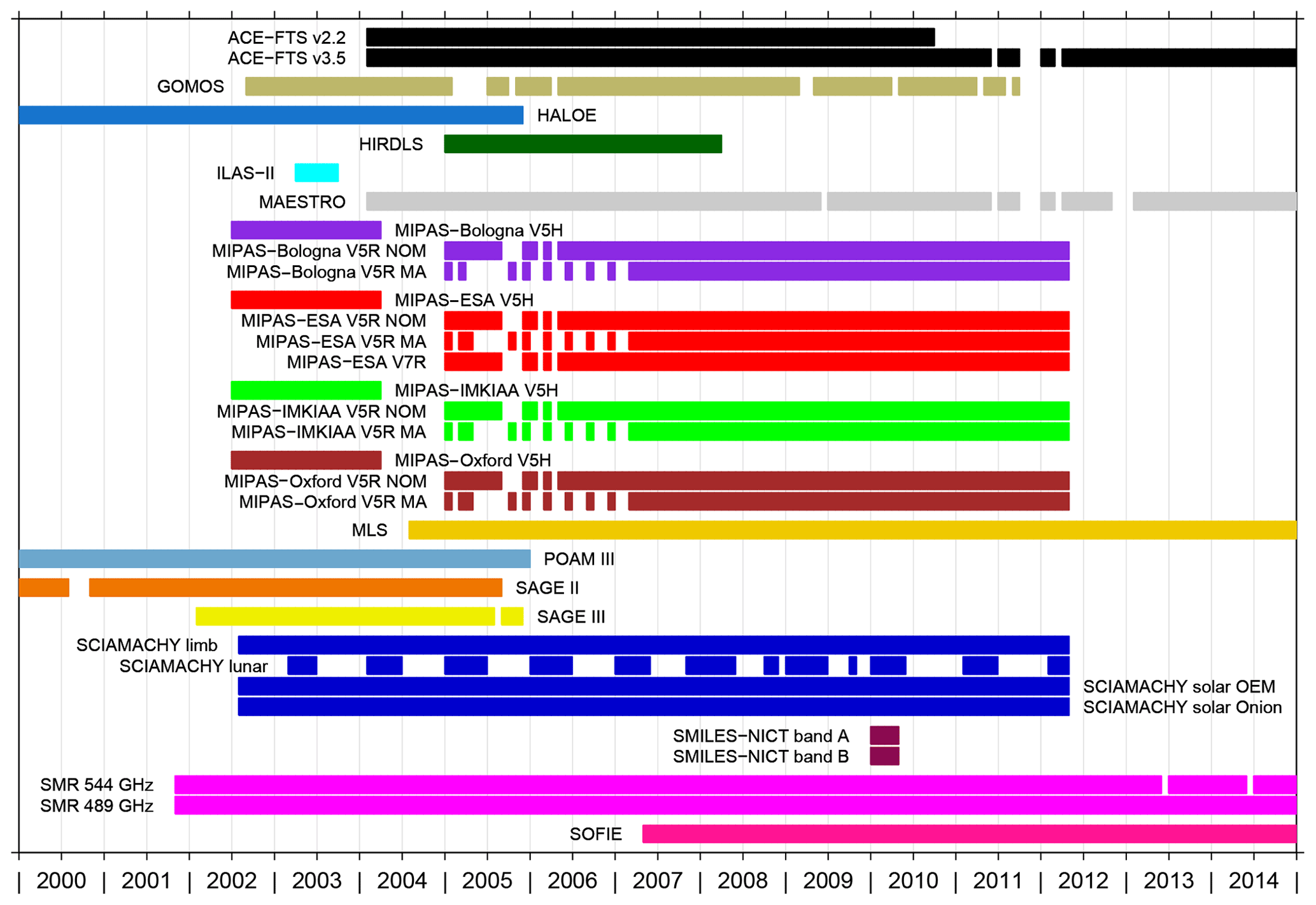
Figure 1The data sets that were included in the comparisons and their corresponding time coverage on a monthly basis. Only data obtained since 2000 are considered.
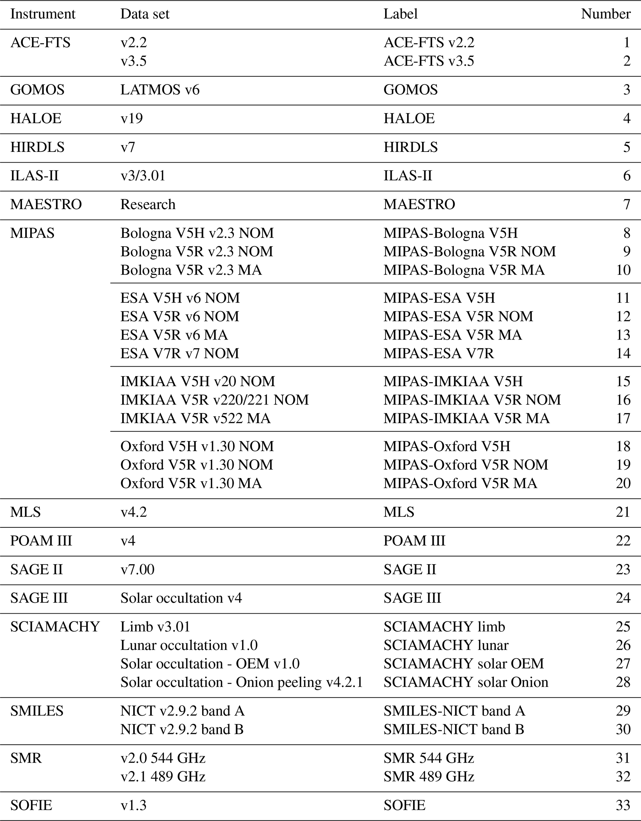
In the present comparisons 33 data sets from 15 individual satellite instruments are considered overall. Table 1 lists them alphabetically with respect to the instrument name. In case of multiple data sets from one instrument, the data sets have been sorted alphabetically (e.g. MIPAS-Bologna data sets before MIPAS-ESA data sets), chronologically (e.g. ACE-FTS v2.2 before ACE-FTS v3.5) or by using a combination of both. The table also lists the corresponding data set labels and numbers that are used in the figures. In addition, Fig. 1 provides a visual overview of the temporal coverage of the individual data sets to give an indication of when coincident observations between two data sets were possible. A complete description of the individual data sets is provided in the WAVAS-II data set overview paper by Walker and Stiller (2019). The focus of the present comparisons is on observations that were acquired since the previous millennium as a follow-up to the last WAVAS report in 2000 (Kley et al., 2000). HALOE, POAM III and SAGE II have provided data in the old millennium but correspondingly those were not considered here. While the SABER observations cover almost the entire time period considered in the assessment no data set has become available and thus they are not part of WAVAS-II. Also, the SAGE III observations from the ISS are not considered as they only commenced in 2017.
Table 1Overview of the water vapour data sets from satellites used in this study.
In a first step we screened the data sets according to the recommendations provided by the individual data set teams. Those screening criteria are listed in full detail in the WAVAS-II data set overview paper (Walker and Stiller, 2019). In addition, we excluded profiles from the comparison that exhibited volume mixing ratios below −20 ppmv or above 50 ppmv anywhere at altitudes above 70 hPa. This wide interval was chosen to reject obvious outliers that might influence the comparisons in an undesirable way and that were not removed by the earlier screening. For many data sets this affected only a handful profiles. In absolute numbers, most profiles were affected for the GOMOS, HIRDLS, MIPAS-Bologna V5R NOM, MIPAS-Oxford and SMR 544 GHz data sets. For the GOMOS data set this meant that about 3.5 % of the profiles were discarded; for the other data sets the percentage was in the per mille range. As a last step we sorted the individual observations of a given data set chronologically.
3.1 Determination of coincident observations
Principally, we considered observations from two data sets as coincident when the following criteria were satisfied:
-
a maximum temporal separation of 24 h
-
a maximum spatial separation of 1000 km
-
a maximum latitude separation of 5∘
-
a maximum equivalent latitude separation of 5∘
When different versions of the ACE-FTS, MIPAS, SCIAMACHY solar occultation and the SMILES data sets were compared with each other these coincidence criteria were not invoked. In these cases the exact same observations were compared. For SMR the different data sets are obtained on different measurement days, so that this exception does not apply. The same is true for MIPAS observations in the nominal mode (NOM) and the middle atmosphere (MA) mode. Also, the different SCIAMACHY observation geometries did not provide simultaneous measurements among them.
To apply the equivalent latitude criterion a scalar value was assigned to every observation. This value was based on an average of equivalent latitudes within the altitude range from 425 to 2000 K potential temperature, which essentially covers the entire stratosphere. The equivalent latitude information was derived from MERRA (Modern Era Retrospective-Analysis for Research and Applications, Rienecker et al., 2011) reanalysis data of potential vorticity.
To determine the coincidences we went through the individual observations of the first data set and determined the observations of the second data set that fulfilled the coincidence criteria. If multiple coincidences were found we chose the coincidence closest in spatial distance. This choice is optimised for the stratosphere, where the diurnal variation is small (Haefele et al., 2008). Close to the tropopause and towards the middle mesosphere the diurnal variation in water vapour becomes more relevant. Once an observation of the second data set was determined to be a coincidence it was not considered any further as a possible coincidence for other observations of the first data set. Inherent in this approach is that the final coincidence pairs are dependent on the choice of the first data set: comparing ACE-FTS and HALOE, for example, can result in different coincidences than when comparing HALOE and ACE-FTS. To avoid inconsistent results based on this aspect, we only derived coincidences for the lower half of the data set comparison matrix and used those results for the upper half of that matrix. According to the sorting of the data sets in Table 1, the ACE-FTS v2.2 data set has been used as first data set in all comparisons. The SMR 489 GHz data set was considered as first data set only in the comparison with the SOFIE data set, while the latter never served as the first data set. We investigated the influence of the first data set choice based on test comparisons with the HALOE, ACE-FTS v2.2 and MIPAS-IMKIAA V5H data sets. Typically the differences in the biases were smaller than 0.05 ppmv or 1 % in absolute and relative terms, respectively. Larger deviations were mostly found at the lower-altitude limits of the comparisons.
3.2 Consideration of different vertical resolutions
The data sets considered in our comparisons have different vertical resolutions. A summary figure and a description of how the resolutions have been estimated is provided in the data set overview paper by Walker and Stiller (2019). Differences in the vertical resolution only play a role for the comparisons at altitudes where the vertical distribution exhibits distinct structures; elsewhere the data sets can be compared directly regardless of the resolution differences. In our work this concerns first and foremost the hygropause region in the lowermost stratosphere. To decide in which comparisons a consideration of differences in the vertical resolution is necessary, we categorised the data sets into various classes according to their vertical resolution dz around the hygropause, using some reasonably selected resolution intervals. These classes are given by the first four columns in Table 2. The lower the class number, the better the vertical resolution of the data sets around the hygropause. The differences in the vertical resolution were considered in those comparisons where the two data sets were in different classes. The data set in the lower class was degraded to the vertical resolution of the data set in the higher class. In the table columns some data sets have been marked by an asterisk, indicating that these data sets have a limited observational coverage of the hygropause. Some retrieved profiles will include the hygropause, while others do not. Hence, some comparisons to these data sets may not necessarily need the consideration of differences in the vertical resolution in this altitude range. Yet, they have been taken into account for completeness.
Table 2The convolution classes. Based on these differences in the vertical resolution were considered in the comparisons of the data sets. The first four classes consider resolution differences around the hygropause, while class V addresses differences at the stratopause and lower mesosphere. Data sets marked by a asterisk have a limited coverage of the hygropause. The consideration of differences in the vertical resolution in comparisons to these data sets may be not necessary but has been made just in case.
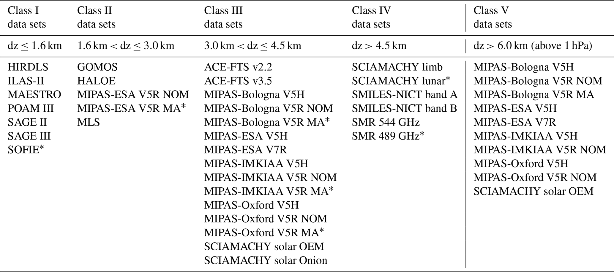
The water vapour maximum in the vicinity of the stratopause is relatively broad and can accordingly be considered less problematic. Yet, some data sets exhibit a strong degradation of their vertical resolution in this altitude region, in particular in the lower mesosphere. To check any influence of this degradation we considered a fifth convolution class that includes data sets with a vertical resolution exceeding 6 km anywhere above 1 hPa in the resolution summary figure presented by Walker and Stiller (2019). The differences in the vertical resolution are considered in the comparisons to those data sets that are not part of this convolution class and which cover altitudes up to at least 1 hPa. The GOMOS, HIRDLS, MAESTRO, SCIAMACHY limb, SMILES-NICT band A, SMILES-NICT band B and SMR 544 GHz data sets do not fulfil the latter criterion.
Due to the focus on differences in the vertical resolution in two different altitude regions, hybrid cases are possible, i.e. comparisons between data sets where one data set is better vertically resolved around the hygropause but worse than the other data set at high altitudes and vice versa. In total there have been 19 such cases in which we made two comparisons considering the differences around the hygropause and at high altitudes individually. The results will be presented later as a combination of these two comparisons. Up to 10 hPa, data from the comparison considering the differences in the vertical resolution around the hygropause are taken into account. Above, the results from the comparison focusing on the resolution differences at the stratopause and the lower mesosphere are used.
The degradation of the higher vertically resolved data sets followed the approach by Connor et al. (1994). Using the averaging kernel A and the a priori profile xa priori of the lower-resolved profile, which we denote collectively as convolution data, the degradation of the higher-resolved profile xhigh can be achieved as follows:
The degraded profile xdeg can then be compared directly to the lower vertically resolved data set. According to the equation the degradation is performed on the grid of the lower-resolved profile. The regridding of the higher-resolved profile to this grid follows the work of Stiller et al. (2012a). For some data sets the averaging kernel considers the log space, i.e. A=Aln, based on a different retrieval approach. In these cases Eq. (1) has to be adapted to (e.g. Stiller et al., 2012a):
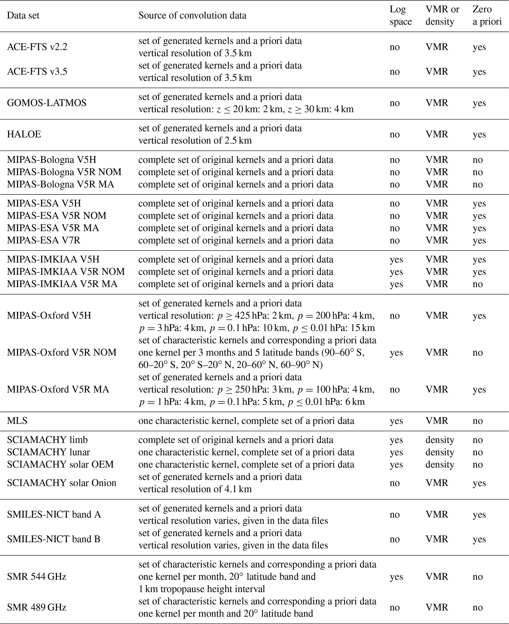
The third column of Table 3, which lists the sources and characteristics of the convolution data employed in our comparisons, indicates the data sets for which this aspect had to be considered. Please note that this is specific to the convolution data employed here. For example, the retrievals of the MIPAS-Oxford V5H and V5R MA data sets are performed in log space. But for these data sets we had to generate the convolution data ourselves (as described below, see the second column of Table 3), which simply assumed a linear space. The degradation of the vertically higher-resolved data sets has been performed in the natural domain of the lower-resolved data sets, as specified in the fourth column of Table 3. Most data sets have volume mixing ratio (VMR) as a natural domain, and only some SCIAMACHY data sets use number density. Again this is specific to the convolution data used in this work. The retrievals of the GOMOS and SCIAMACHY solar Onion data sets, for example, use number density as the natural domain, but once more we needed to generate the corresponding convolution data which assumed volume mixing ratio as the natural domain. Temperature and pressure data for the conversion between volume mixing ratio and number density have been provided by all data set teams, either retrieved from the same set of measurements or from an auxiliary data source as reanalysis. Walker and Stiller (2019) provide a comprehensive summary of the retrieval spaces and domains of the individual data sets as well as the sources of the additional temperature and pressure information.
Table 3Sources and characteristics of the convolution data used in the comparisons.
Another aspect is that the convolution data often exceed the altitude range covered by the particular profile to be degraded. This can be handled by either reducing the altitude range of the convolution data or extending the altitude range of the profile to be degraded. For that, a priori or other climatological data as well as model simulations can be employed. In practice the latter approach is often the better choice, leading to more reasonable results at the vertical boundaries of the degraded profile. After the degradation the extension data are removed again. Here, we utilised offset-corrected, climatological data from HAMMONIA (Hamburg Model of the Neutral and Ionized Atmosphere, Schmidt et al., 2006) as a function of month and latitude.
The second column of Table 3 lists the sources of the convolution data that have been employed in the comparisons. For most MIPAS data sets and the SCIAMACHY limb data set, the complete set of averaging kernels and the corresponding a priori data were available. A single characteristic averaging kernel and observation-dependent a priori data were provided for the MLS, SCIAMACHY lunar and solar OEM data sets. For the MIPAS-Oxford V5R NOM data set and both SMR data sets, collections of characteristic averaging kernels were supplied. They are dependent on time and latitude band. For the SMR 544 GHz data set there is also a dependency on the tropopause altitude. This data set only covers the upper troposphere and lower stratosphere, and the tropopause altitude is the main source of kernel variability. Since for the SMR data sets the convolution data are not saved by default, we re-retrieved the convolution data from at least 20 (50) observations that fell into the individual bins (monthly and 20∘ latitude; see Table 3) for the 544 GHz (489 GHz) data set. For those bins where overall fewer observations exist we re-retrieved all of them. From this set we selected the convolution data for which the averaging kernel minimised the following quantity as being the most representative:
Here, Ad denotes the averaging kernel diagonal that has been interpolated on a regular altitude grid prior to the analysis. is the average averaging kernel diagonal over the entire set of re-retrieved data for a particular bin and j is the index over the altitude levels lstart, …, lend that were considered. For the 544 GHz data set we took into account the altitude range between 10 and 25 km, while for the 489 GHz data set the altitude range between 15 and 50 km was considered.
For the remaining data sets averaging kernels are typically not part of their retrieval or were not provided to us. The latter applies to the MIPAS-Oxford V5H and V5R MA data sets. In these cases we generated averaging kernels ourselves based on Gaussian functions, using volume mixing ratio as the natural domain (as noted above) and kept the a priori constant at zero. The averaging kernel row Ar(j) for a given altitude index j was calculated as follows:
with
In the equation na represents the number of altitudes contained in the altitude vector z. Accordingly z(j) is the altitude for which the averaging kernel row is calculated and dz(j) describes the vertical resolution at this altitude. The vertical resolutions that have been used to generate the averaging kernels of the individual data sets are also given in the second column of Table 3. For the MIPAS-Oxford V5H and V5R MA data sets the vertical resolutions have been assumed, while for the other data sets they are typically based on the field of view. The only exceptions are the GOMOS and the SCIAMACHY solar Onion data sets. For the latter the vertical resolution is based on the smoothing of the absorption profiles, while the estimate for the GOMOS data set relied on actual averaging kernels. As altitude vector we considered the altitudes given in the data files for the individual observations. For the ACE-FTS data sets we used the data files with the tangent altitude grid and not those with the interpolated regular 1 km grid. When generating the averaging kernel for a given observation we set rows to zero for those altitudes where data were missing, either due to a lack of coverage or screening.
3.3 Derivation of biases between the data sets
The comparisons essentially followed the approach outlined by Dupuy et al. (2009), which compared various ozone data sets. The bias between two coincident data sets for a given time period t and latitude band ϕ and for a specific altitude z has been calculated as
where denotes the corresponding number of coincident measurements and are the individual differences between them. These differences were considered both in absolute,
and relative terms
where are the individual water vapour abundances of the first data set and are the abundances of the second data set. As reference for the relative bias, several options were possible, like the first data set, the second data set in a comparison or the mean of the two data sets. In our work we used the last option. A reason for the decision was that satellite observations can have larger uncertainties and thus the mean may be a more appropriate choice (Randall et al., 2003; Dupuy et al., 2009). Another aspect was simply convenience. For a specific comparison there is no need to know which data set acted as reference. Eventual inconsistencies based on the combination of which data set was chosen to be the first data set in the comparison (see Sect. 3.1) and which one was used as reference can be avoided. Finally, we also wanted to intentionally avoid any preference towards using a certain data set as reference but to compare all data sets on equal terms. Accordingly, the relative biases presented here are not comparable to those shown in the first SPARC water vapour assessment (Kley et al., 2000), where the HALOE data set was always used as reference. In general, any a posteriori attempt to relate the relative bias to the first or the second data set (instead of the mean among the data sets) is not meaningful nor appropriate, because there is some non-intuitive behaviour involved according to Eq. (8). A simple example for that is provided in the Appendix.
Before the mean bias was derived we performed an additional screening on the individual biases using the median and median absolute deviation (MAD, e.g. Jones et al., 2012). After screening profiles with data points outside a reasonable abundance range, as described in Sect. 2, this is a second attempt to ensure meaningful bias estimates. We preferred this method over a screening using the mean and standard deviation due to its superior robustness with respect to larger outliers. Individual biases outside the interval 〈median[] ± 10 × MAD[]〉, with i=1, …, , were discarded. For a normally distributed set of data, 10 × MAD corresponds roughly to 7.5 standard deviations. Hence this has not been a very strict screening, aiming to remove the most prominent outliers of individual biases .
As indicated by Eqs. (6)–(8) the biases were calculated for various sets of coincidences covering different time periods t and latitude bands ϕ as listed below:
-
time t: MAM, JJA, SON, DJF and all seasons together
-
latitude ϕ: 90–60∘ S (also referred to as Antarctic), 60–30∘ S, 30∘ S – Equator, 15∘ S–15∘ N (also referred to as tropics), Equator – 30∘ N, 30–60∘ N, 60–90∘ N (also referred to as Arctic) and 90∘ S–90∘ N (also referred to as global).
The comparisons were performed on pressure as altitude scale and biases have been derived in the volume mixing ratio space. For this all data sets were interpolated on a common grid with 32 levels per pressure decade. Tropospheric data were intentionally removed using MERRA tropopause information. Comparisons in the troposphere will be presented by Read et al. (2019). Due to the finite vertical resolution of the individual data sets the removal of tropospheric data has not been perfect and at the lower boundary volume mixing ratios still remain that are associated with tropospheric conditions. In comparisons where differences in the vertical resolution among the data sets had to be considered, the tropospheric data were removed after the convolution to obtain optimal results. In the following figures, we only show bias results that are based on at least 20 coincidences to avoid spurious results. This primarily targets the lower and upper vertical limits of the comparisons, where typically the smallest numbers of coincidences tend to occur.
Given the large number of data sets, this work yields a large number of comparisons. Even though every comparison is unique, some sort of combination is needed to be able to present the results in a reasonable way. To summarise the bias results for a given data set considering a specific time and latitude band, we chose the median over all available comparisons (with an aggregation of the MIPAS results as described later in Sect. 3.5). We tested other approaches but the median appeared to be the optimal choice for multiple reasons. It provides robust statistics in the presence of outliers (avoiding the need for additional screening) and it does not require any assumption of a certain probability distribution or a specific weighting of the individual comparisons.
3.4 Drift analysis
Besides the bias estimation we performed an analysis of drifts among the different data sets. Unlike for the bias comparisons, we do not separate the drift comparisons by season. The drift analysis was based on monthly averaged biases derived from a minimum of five coincidences. Drifts were only calculated if the overlap period between the two data sets compared was at least 36 months. This period is defined as the time between the first and the last month where sufficient coincidences were found between the two data sets. The estimation of the drifts was done with a regression model that contained an offset, a single linear term for the drift as well as terms for the semi-annual (SAO), annual (AO) and quasi-biennial oscillation (QBO):
In the equation, represents the fit of the regressed bias time series ; however here t describes all months in which the data sets that are compared have sufficient overlap (i.e. five coincidences; see above). C are the regression coefficients of the individual model components and Cdrift describes the drift that is sought. The SAO and AO are parameterised by orthogonal sine and cosine functions, while for the QBO the normalised winds at 50 hPa (QBO1) and 30 hPa (QBO2) observed over Singapore (1∘ S, 104∘ E) are used. These winds are closely orthogonal and have been compiled by Freie Universität Berlin (web page: http://www.geo.fu-berlin.de/met/ag/strat/produkte/qbo/qbo.dat, last access: 16 April 2019). pSAO and pAO represent the time periods of the semi-annual (0.5 years) and annual variation (1 year), respectively. The regression coefficients were derived following the method by von Clarmann et al. (2010) using the standard mean error of the monthly averaged biases as statistical weights. In the regression autocorrelation effects and empirical errors are also considered, using the same approach as outlined by Stiller et al. (2012b).
In our work we consider drifts as statistically significant when they exceed the 2σ uncertainty level. σ is defined as the absolute ratio between the drift estimate Cdrift and its uncertainty ϵdrift:
3.5 Aggregation of the MIPAS results
The previous WAVAS-II papers (Lossow et al., 2017; Nedoluha et al., 2017; Khosrawi et al., 2018) often received comments on the large number of MIPAS data sets (here 13 out of 33; see Table 1 for example) included in the assessment. As described in these publications the different MIPAS data sets are based on different measurement modes (with different vertical sampling) and, more prominently, are derived by four different processors with varying retrieval choices, as microwindows, vertical grid regularisation, spectroscopic database or a priori, for example. Here, we want to provide general results in the form of percentiles and histograms using all comparison results as well as summaries of data-set-specific biases as described at the last paragraph of Sect. 3.3. In general such results will always depend on the data sets that are considered. One of the WAVAS-II goals was to involve as many data sets as possible to provide a complete and realistic picture. There are, however, limits. For example, if all data sets in such an assessment were experimental (i.e. test or research versions), any general result derived from the combination of them would be rather meaningless. Also, the large number of MIPAS data sets in our assessment may be such a limit. Accordingly, we asked ourselves if our intended results may be influenced or skewed by the large number of MIPAS data sets. The typical biases among the different MIPAS data sets are significantly smaller than among the non-MIPAS data sets. They amount to roughly 0.1 ppmv (0.5 ppmv) for the MIPAS (non-MIPAS) data sets, considering large parts of the stratosphere. A similar picture is found in terms of typical drifts. In the stratosphere they are approximately 0.1 ppmv decade−1 for the MIPAS data sets, while for the non-MIPAS data sets they correspond to 0.3 ppmv decade−1. This indicates a relative similarity among the different MIPAS data sets in contrast to the non-MIPAS data sets. This can clearly affect our intended general results based on all comparison results. In addition, the summary biases (based on the median over all comparisons to the other data sets; see Sect. 3.3) for any randomly picked MIPAS data set will be small because this data set is compared with many relatively similar ones. In contrast, a single non-MIPAS data set has to be compared with the bulk of the MIPAS data sets. If these comparisons disagree, the summary biases for this non-MIPAS data set will be large. Given these considerations we decided to aggregate the MIPAS results. For percentiles, histograms and full matrix plots, the aggregation has been performed as follows:
-
All MIPAS comparison results to a given non-MIPAS data set are combined using the median.
-
Comparison results between different MIPAS data sets are not considered (in the calculation of the aggregated quantities).
For the summary bias of a given data set, described in Sect. 3.3 and shown in Figs. 8 and 9 in the main paper as well as in Fig. S9 in the Supplement, the following approach has been chosen:
- (a)
For a non-MIPAS data set, like HALOE
where represents all biases of the HALOE data set to the remaining non-MIPAS data sets and describes the HALOE biases relative to all MIPAS data sets.
- (b)
For a given MIPAS data set, like MIPAS-Bologna V5R NOM
where are all the biases to non-MIPAS data sets and represents the biases of the MIPAS-Bologna V5R NOM data set to the remaining MIPAS data sets.
In numerous figures we supply as auxiliary information the number of comparisons or data points contributing to the results presented. Even when the MIPAS results are aggregated we still count the contributing results individually and do not condense them into a single contribution. For example, in Fig. 9 the bias summaries for the ACE-FTS v3.5 data set are presented. This data set could be compared with all 13 MIPAS data sets if coincidences at all seasons and latitudes are considered. Hence the number of comparisons contributing to these summary biases given in that figure (i.e. 31) includes these 13 comparisons.
We will show some results with and without the aggregation of the MIPAS results for the sake of comparison. In the main paper this concerns Figs. 4, 5 and 11. In the Supplement, Figs. S2, S5 and S10 show percentiles and histograms without the aggregation of the MIPAS results that correspond to Figs. 6, 7 and 12 in the main paper which take this aggregation into account. The two ACE-FTS and SCIAMACHY solar occultation data sets are also based on the same set of measurements. Therefore an aggregation of these results could also be considered. However, due to the small number of the data sets concerned (in relation to the MIPAS data sets), this has not further been pursued.
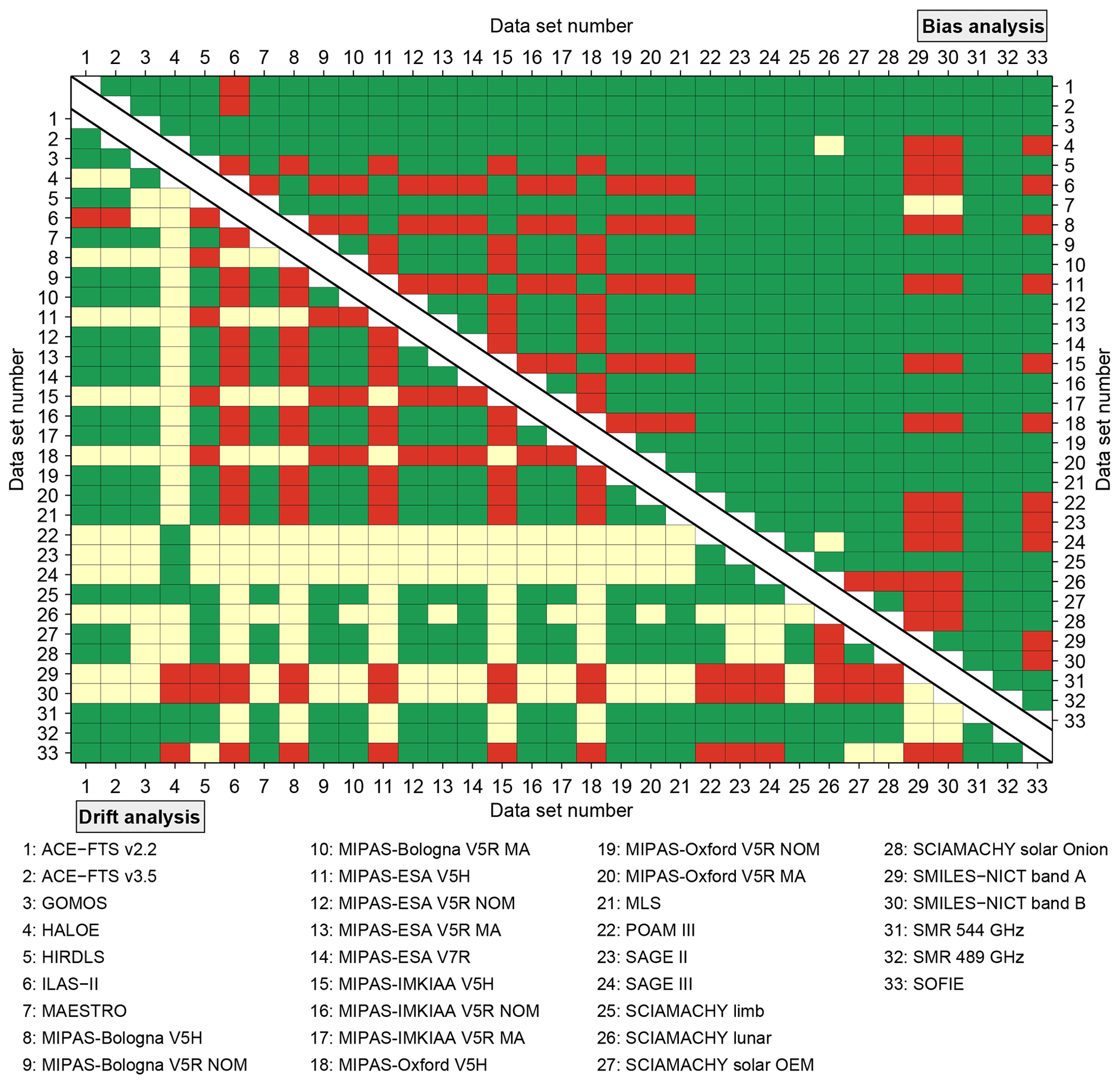
Figure 2Overview which data sets were compared with each other in terms of biases (upper triangle) and drifts (lower triangle). Green means that comparisons were performed, while red indicates that this was not the case. Yellow means that comparisons were performed but the results were not considered any further since they did not meet the minimum criteria we defined in Sect. 3. For the bias comparisons this concerns the minimum number of coincidences (i.e. 20; see Sect. 3.3), while for the drift comparisons this involves the minimum overlap period (i.e. 36 months; see Sect. 3.4).
The presentation of the bias results is split into three parts. We start with an example to provide a first impression of the analyses. Then, we focus on a general, data-set-independent assessment of the biases. This aims to provide a picture of the typical bias characteristics found in the observational database. In the last part of this section, specific results for individual data sets are presented.
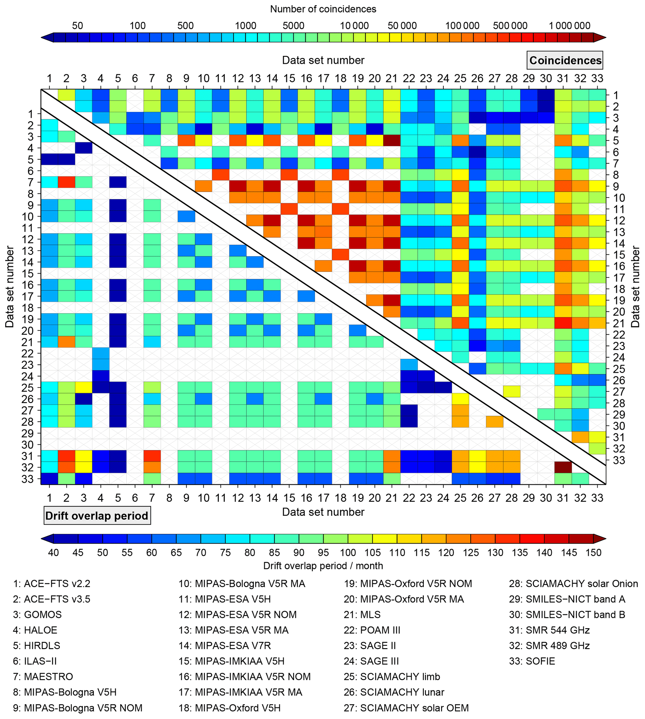
Figure 3Overview of the number of coincidences (upper triangle) and the drift overlap period (lower triangle) between the compared data sets. All numbers consider the comparisons that take into account coincidences during all seasons and at all latitudes. White boxes with grey crosses indicate that no comparison results are available (either yellow or red in Fig. 2).
The upper triangle of Fig. 2 provides a quick overview of which data sets were compared in terms of biases for any of the time–latitude bins considered (see Sect. 3.3). The presentation uses a traffic light system:
-
Green means comparisons were made.
-
Yellow means comparisons were made. However, the minimum criterion of at least 20 coincidences (as defined in Sect. 3.3) was not met at any considered altitude. This concerns four comparisons, namely the comparisons of the HALOE and SAGE II data sets with the SCIAMACHY lunar data set and the comparisons of the MAESTRO data set with both SMILES data sets.
-
Red means no comparison could be made as the data sets do not overlap.
Complementary to this, Fig. 3 shows the number of coincident observations among the data sets (considering all seasons and latitude bands). The HIRDLS and MLS data sets yield more than 3 million coincidences according to our criteria, the largest number found in our comparisons. The comparisons among the different MIPAS V5R NOM data sets comprise more than 1.7 million coincidences. On the opposite end, less than 100 coincident observations are found in the comparisons of the following data sets: ACE-FTS vs. SMILES, GOMOS vs. SCIAMACHY occultation (both lunar and solar), GOMOS vs. SMILES, HALOE vs. MIPAS V5R MA, ILAS vs. SCIAMACHY lunar, MAESTRO vs. SCIAMACHY lunar as well as SAGE II vs. SCIAMACHY lunar.
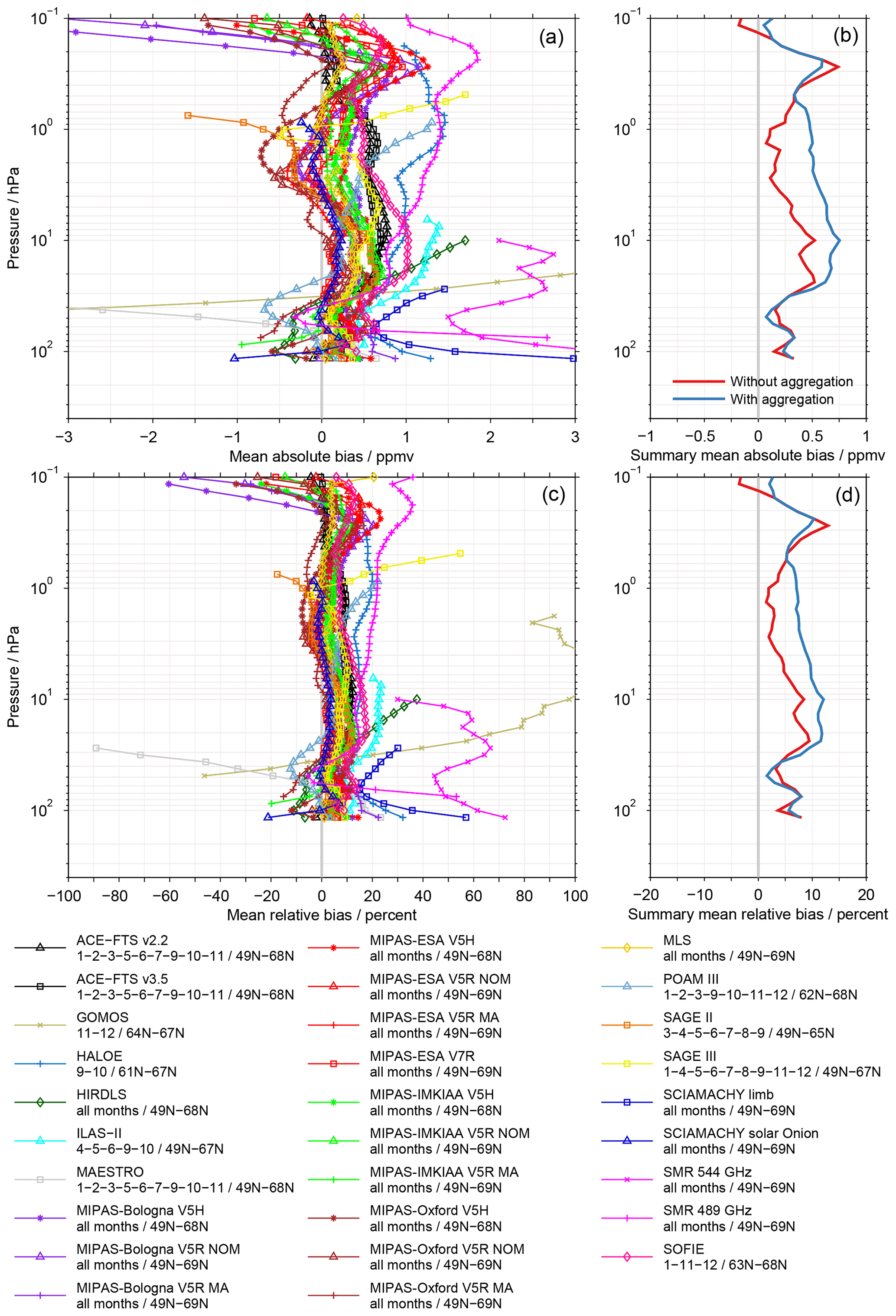
Figure 4Biases of the SCIAMACHY solar OEM data set in absolute (a, b) and relative terms (c, d). These example results are based on coincident observations during all seasons and at all latitudes. Panels (a), (c) show the mean biases to the individual data sets, as listed in the legend. In addition, the legend provides information on the temporal and spatial coverage of the individual comparisons. Panels (b), (d) provide a summary of the bias results. The red profile is based on the median over all comparisons, while the blue profile considers the aggregation of MIPAS results as described in Sect. 3.5. The latter profile is used in Sect 4.3 and in the Supplement to summarise the bias results for the individual data sets. For better visibility only results at every second altitude are plotted (see Sect. 3.3).
4.1 Example
Figure 4 shows exemplarily biases of the SCIAMACHY solar OEM data set, considering coincident observations during all seasons and at all latitudes. The upper row considers biases in absolute terms, while the lower row focuses on biases in relative terms. Figure 4a and c show the biases to the individual data sets (i.e. SCIAMACHY solar OEM minus the other data set; see Sect. 3.3). Figure 4b and d shows the corresponding summary biases. The red profile is based on the median over all comparisons (see Sect. 3.3). The blue profile, additionally, considers the aggregation of MIPAS results as described in Sect. 3.5 and is also used for the summary of the data-set-specific results presented later in Sect. 4.3 and the Supplement. The legend provides information on the actual temporal and spatial coverage of the individual comparisons as a complement. Even though all latitudes are considered in the analysis, the comparisons are limited to the latitude range between 49 and 69∘ N according to the coverage of the SCIAMACHY solar OEM data set.
The comparisons indicate biases of the SCIAMACHY solar OEM data set that are typically within ±1 ppmv or ±20 % in relative terms. In most cases the biases are positive, but in some comparisons also negative biases are found. These negative biases are visible in the lower (roughly between 100 and 50 hPa) and upper stratosphere (between 3 and 1 hPa) as well as in the lower mesosphere (roughly above 0.2 hPa). In the uppermost altitude range this behaviour is systematically observed in comparisons to the MIPAS-Bologna data sets derived from the nominal mode observations, i.e. MIPAS-Bologna V5H and MIPAS-Bologna V5R NOM. For the other altitude ranges no such data-set-specific behaviour is observed. Beyond that, these example biases indicate more issues with specific data sets that will be presented more comprehensively in Sect. 4.3 and the Supplement.

Figure 5(a, c) Bias results for the full matrix of comparisons considering coincidences during all seasons and at all latitudes. Panel (a) shows the absolute biases; panel (c) shows the relative biases. The grey profiles do not consider the aggregation of the MIPAS results, while the light blue profiles do. (b, d) The 50 % (median), 80 % and 95 % percentiles derived from the positive part of the biases shown in (a, c), with and without the aggregation of the MIPAS results.
In accordance with the individual bias results presented in Fig. 4a and c, the summary profiles shown in Fig. 4b and d generally indicate positive biases for the SCIAMACHY solar OEM data set compared with the other data sets. From the summary biases we find that the results are clearly influenced by the summary approach in the altitude range between 30 and 0.6 hPa. Here, the median over all comparisons yields consistently lower biases than the median considering the aggregation of the MIPAS results. Differences between these two profiles become as large as 0.4 ppmv, corresponding to 6 % in relative terms. This highlights the influence that the large number of MIPAS data sets can have in the comparisons, as discussed in Sect. 3.5. The summary profiles considering the aggregation of the MIPAS results exhibit the smallest biases below 25 hPa (around 0.25 ppmv or 5 %) and at 0.1 hPa (about 0.1 hPa or 2 %–3 %). At 10 hPa, and more prominently at 0.25 hPa, the biases maximise. At 10 hPa the bias amounts to 0.75 ppmv or 12 %, while the maximum in the lower mesosphere (also notable in the summary profiles without aggregation) exhibits smaller values (0.6 ppmv or 10 %). On average, the biases amount to 0.5 ppmv (about 8 %) in the stratosphere.
4.2 General results
Figure 5a and c show the biases from the full matrix of comparisons. Here, the comparisons that include coincident observations during all seasons and at all latitudes are considered. Figure 5a and b show the results for the absolute biases. In Fig. 5c and d the results for the relative biases are given. Based on our comparison approach (see Sect. 3.1) the results for the full matrix are symmetric around zero. In grey the comparison results without the aggregation of the MIPAS results are shown. With 33 data sets, theoretically comparisons (of which 528 are unique) are possible. But since not all data sets overlap with each other the actual number decreases to 862 comparisons (of which 431 are unique; see Fig. 2). For eight comparisons (four unique) the biases are based on less than 20 coincidences at all altitudes and were thus not considered any further (see Sect. 3.3 or description of Fig. 2 in the beginning of this section). Hence, the unaggregated results are effectively based on 854 comparisons (427 unique). In blue the comparison results considering the aggregation of the MIPAS results are shown. As described in Sect. 3.5 the aggregation omits comparisons among the MIPAS data sets, reducing the amount of available comparisons to 770. After combining all MIPAS results in comparisons to non-MIPAS data sets, 348 comparisons remain for the full matrix.
Overall, the left column of Fig. 5 provides a good first impression of the typical envelope of biases in the observational database. Above 30 hPa the biases are typically within ±2 ppmv (or ±40 %). Below this altitude the biases can get significantly larger and even exceed ±5 ppmv or ±100 % on some occasions.
Based on the positive biases shown in (a, c) of Fig. 5, (b, d) show the corresponding 50 % (i.e. median, blue), 80 % (green) and 95 % (red) percentiles without (lighter colours) and with (darker colours) the aggregation of the MIPAS results. In general, the 50 % and 80 % percentiles are quite constant above 70 hPa, while the 95 % percentile shows much more variation in this altitude range. At altitudes below there is a distinct increase in the corresponding values. In addition, the percentiles considering the aggregation of the MIPAS results are larger than without this aggregation. At stratospheric altitudes the differences amount to 0.1 ppmv (2 %) for the 50 % percentile, 0.2 ppmv (5 %) for the 80 % percentile and 0.5 ppmv (7 %) for the 95 % percentile. Prominent exceptions from this behaviour are observed close to 0.1 hPa, below 200 hPa (except for 50 % percentile of the absolute biases) or between 2 and 1 hPa for the 95 % percentile of the absolute biases. In the following description we focus on percentiles considering the aggregation of the MIPAS results. The 50 % percentile is around 0.5 ppmv above 100 hPa and minimises at 60 hPa with 0.35 ppmv. Below 200 hPa the 50 % percentile exceeds 2 ppmv. In relative terms, the 50 % percentile is smaller than 10 % around 60 hPa and between 25 and 0.3 hPa. From 100 to 250 hPa the 50 % percentile increases from 12 % to 40 %. Below, the percentile actually decreases again to reach a pronounced minimum of 23 % at about 340 hPa. The 80 % percentile, considering the absolute biases, averages to 1.1 ppmv for altitudes above 100 hPa. A distinct minimum is again observed at 60 hPa (0.8 ppmv). Also, in the altitude range between 10 and 3 hPa, as well as around 0.5 and 0.1 hPa, pronounced minima of about 1 ppmv are visible. At 100 hPa the 80 % percentile amounts to 1.5 ppmv. With decreasing altitude it quickly increases and exceeds 5 ppmv slightly below 200 hPa. For the relative biases the 80 % percentile varies between 20 % and 35 % in the altitude range between 100 hPa and 10 hPa. Higher up, it is below 20 % with a few exceptions. Below 200 hPa the 80 % percentile ranges from 50 % to 70 %. Again a pronounced minimum is observed close to 370 hPa, similar to that observed for the 50 % percentile. The 95 % percentile is generally smaller than 2 ppmv with three noticeable exceptions. One concerns the altitude range below 70 hPa, in a similar fashion to that observed for the other two percentiles. Another exception is observed around 30 hPa, where a localised maximum of more than 5 ppmv is found. This behaviour can be attributed to the MAESTRO data set that is close to its upper boundary and exhibits high positive biases at these altitudes. The third exception is visible at 0.7 hPa, primarily attributed to the two SAGE data sets. In relative terms, the 95 % percentile ranges from 20 % to almost 80 % above 70 hPa. Below 100 hPa there are large variations and the values exceed 100 % occasionally.
To provide a more quantitative statement on how variable these percentiles are we applied a jackknife approach (Efron, 1979). Randomly we left out five data sets and recalculated the percentiles. We repeated this until every data set had been left out at least once. This approach yields a set of results (typically about 25 for the non-aggregated data and a dozen for the aggregated data) for a given percentile. From this set of results a standard deviation can be calculated. Given our random approach many different sets of results (and corresponding standard deviations) are possible. One characteristic realisation is shown in the Supplement in Fig. S1. Overall, standard deviations are in general around 0.05 ppmv (1 %) for the 50 % percentile without the aggregation of the MIPAS results. With this aggregation the standard deviations are typically twice as large in the stratosphere. Close to 0.1 hPa standard deviations around 0.25 ppmv (4 %) are observed. For the 80 % percentile the standard deviations amount roughly to 0.1 ppmv (1 %–5 %) and 0.2 ppmv (2 %–10 %) without and with the aggregation of the MIPAS results, respectively. For the 95 % percentile the standard deviations vary typically between 0.05 and 0.5 ppmv (2 %–10 %) when no aggregation of the MIPAS results is considered. If the aggregation is taken into account a larger variation is observed with peak values exceeding 1 ppmv (20 %).
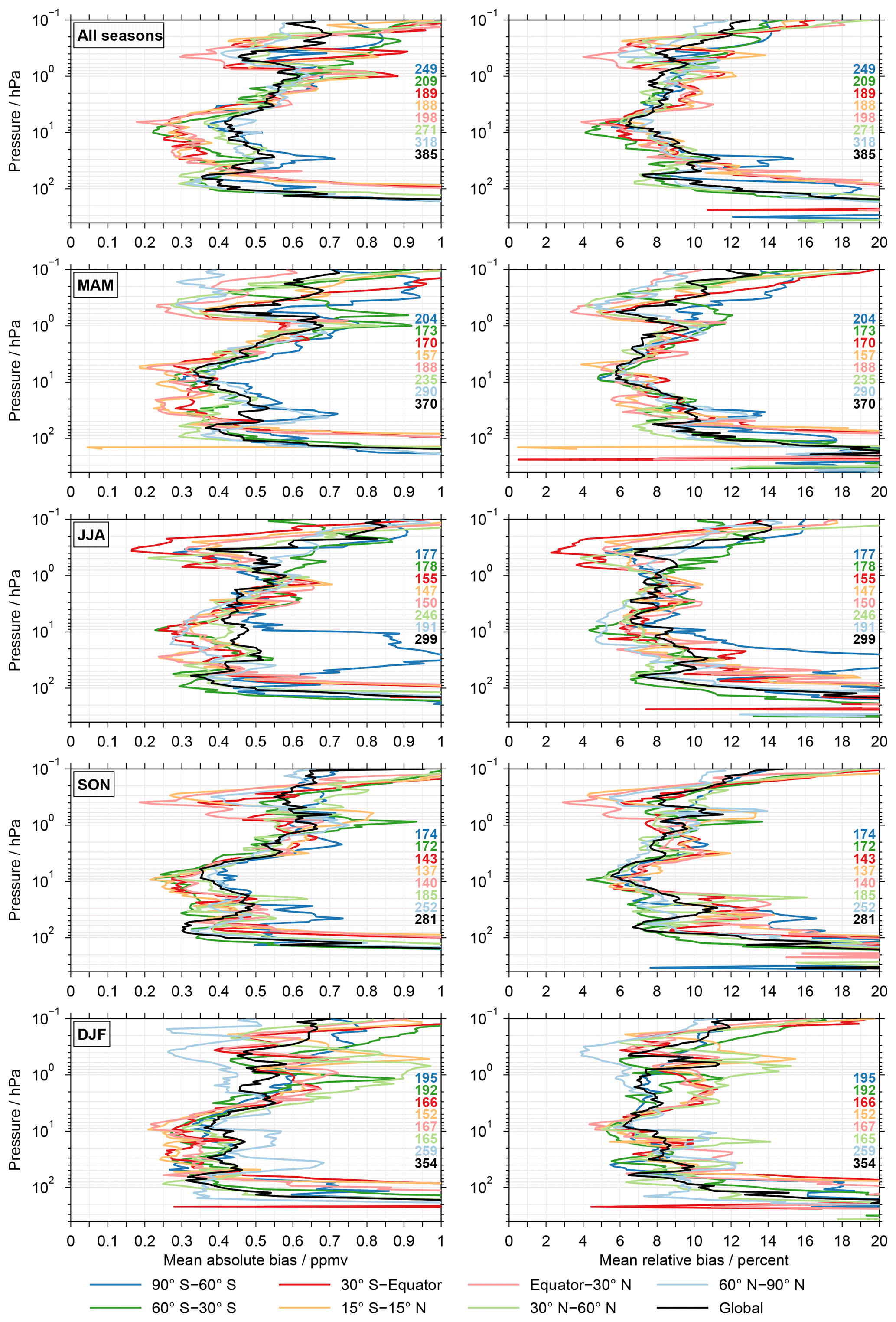
Figure 6The 50 % percentile (median) of the biases from all available comparisons for different times and latitude bands, considering the aggregation of the MIPAS results. The left column considers the absolute biases, the right column the relative biases. The different rows focus on individual seasons or their combination. The results for the different latitude bands are colour coded. On the right-hand side of the individual panels the number of comparisons contributing to the results are indicated. Here, the comparisons with the different MIPAS data sets are counted individually and not combined into a single comparison.
In Fig. 6 the characterisation of the typical biases is extended by considering the 50 % percentile (median) for different seasons and latitude bands. These results take into account the aggregation of the MIPAS results and are again based on the positive biases only, as the percentile results shown in the previous figure. The left column of the figure considers the absolute biases, the right column focuses on the relative biases. The different rows focus on different seasons or their combination. The results for the different latitude bands are colour coded. On the right side of the individual panels the number of (unique) comparisons contributing to the results are given. As described in Sect. 3.5, the comparisons to the different MIPAS data sets are counted individually. In general, the 50 % percentiles exhibit a rather common altitude dependence for the different seasons and latitude bands. Below about 70 hPa the 50 % percentiles increase considerably and the highest values are observed in the tropics and subtropics. Below 200 hPa the values are typically beyond the upper limits of the x axes considered here, i.e. 1 ppmv in absolute terms and 20 % in relative terms. The 50 % percentiles are typically lowest in the altitude range from roughly 70 to 5 hPa. The values here vary between 0.25 and 0.5 ppmv in absolute terms and between 5 % and 10 % in relative terms. In this altitude region, the lowest values generally occur outside the polar regions. Higher up, there is a distinct increase of the 50 % percentiles, i.e up to about 1 hPa. At this altitude the 50 % varies approximately between 0.6 and 0.8 ppmv (roughly 8 % to 12 %). In JJA the values are a bit smaller, while in DJF there is a much larger variation among the latitude bands (percentiles minimise for the Arctic and maximise for the latitude band from 30 and 60∘ N). Higher up, the 50 % percentiles vary considerably with altitude and among the latitude bands, comprising values from 0.3 to 1 ppmv (4 % to 20 %). The smallest values are typically observed between 0.5 and 0.4 hPa. In MAM, SON and all seasons combined, the latitude band from the Equator to 30∘ N stands for these minimum values. In DJF this occurs prominently in the Arctic. The largest values are observed at 0.1 hPa, with pronounced variations among seasons and latitude bands.

Figure 7Histograms of the absolute (left column) and relative biases (right column) considering results from the entire altitude range. As in the previous figure the different rows consider different seasons, while the different latitude bands are colour coded in the individual panels. Also, these histograms take into consideration the aggregation of the MIPAS results. The increase at the right end of the panes comes from the integration over all biases larger than 3 ppmv and 50 %, respectively.
Figure S2 in the Supplement shows the results corresponding to Fig. 6 without the aggregation of the MIPAS results. Overall, the altitude dependence is quite similar to the results shown here. However, without the aggregation, the values for the 50 % percentiles are smaller (like in Fig. 5), as is the variation among the different latitude bands and seasons (a prominent exception occurs at 0.1 hPa). To further complement Fig. 6, the results for the 80 % and 95 % percentiles, again considering the aggregation of the MIPAS results, are shown in the Supplement (Figs. S3 and S4). For these larger percentiles the altitude dependence is somewhat different, in particular for the 95 % percentile, where less pronounced differences between stratospheric and lower mesospheric values are visible. Pronounced differences among the latitude bands occur in the lower stratosphere rather than the lower mesosphere.
For a last characterisation of the biases in the observational database we use histograms, as shown in Fig. 7. These results again use the positive biases only, consider data from all altitudes and take into account the aggregation of the MIPAS results. The histograms for the absolute biases (left column) use bins of 0.1 ppmv. For the relative biases (right column), bins of 2 % are considered. As in the previous figure the different panels consider different seasons or their combination. The different latitude bands are again colour coded. On the right side of the individual panels the number of data points contributing the results are given (again comparisons to different MIPAS data sets are counted individually; see Sect. 3.5). Overall, the histograms exhibit a similar picture for the different seasons and latitude bands. The occurrence rates typically maximise within the first bin that ranges from 0 to 0.1 ppmv (between 11 % and 13 %). The decrease in occurrence towards larger biases (up to 0.8 ppmv) is steepest in DJF. For biases around 1 ppmv the occurrence has dropped to 2.5 % to 4.5 %. Biases beyond 3 ppmv occur in 2 % to 7 % of the comparisons. The lowest occurrences for these biases are observed in the Antarctic and tropics. In relative terms the occurrence of biases within the first bin from 0 % and 2 % varies between 10 % and 14 % depending on season and latitude band. A bias of 10 % occurs in about 6 % to 9 % of the comparisons. For biases beyond 50 % the occurrence is typically between 2 % and 8 %. The lower limit is observed for the latitude band between 30∘ S and the Equator in JJA. In contrast, the upper limit occurs in the Antarctic in DJF.
As for the previous figure we present the results without the aggregation of the MIPAS results, corresponding to Fig. 7, in the Supplement (Fig. S5). The results without the aggregation exhibit larger occurrence rates for the smallest biases (between 14 % and 19 %). Besides that, the variation among the different latitude bands is smaller. In addition, in the Supplement we present histograms that focus separately on data in the altitude ranges 100–10 hPa, 10–1 hPa and 1–0.1 hPa (see Figs. S6, S7 and S8), again considering the aggregation of the MIPAS results. The picture in the altitude range from 100 to 10 hPa is relatively similar to that observed in Fig. 7. In the altitude range from 10 to 1 hPa, the maximum occurrence rates occur over a larger bias range (roughly up to 0.5 ppmv or 10 %). Occasionally there are pronounced peaks in the occurrence rate, often involving data in the tropics and subtropics. Biases beyond 3 ppmv or 50 % occur more rarely than in the altitude range from 100 to 10 hPa. This behaviour is even more obvious in the altitude range from 1 to 0.1 hPa. Here, the histograms exhibit a pronounced variation among the different latitude bands. The smallest biases often show very high occurrence rates. Within the next bins a steep decrease in the occurrence rates is observed. Pronounced secondary maxima in the occurrence rates occur for biases beyond 0.5 ppmv or 10 %, depending on season and latitude.
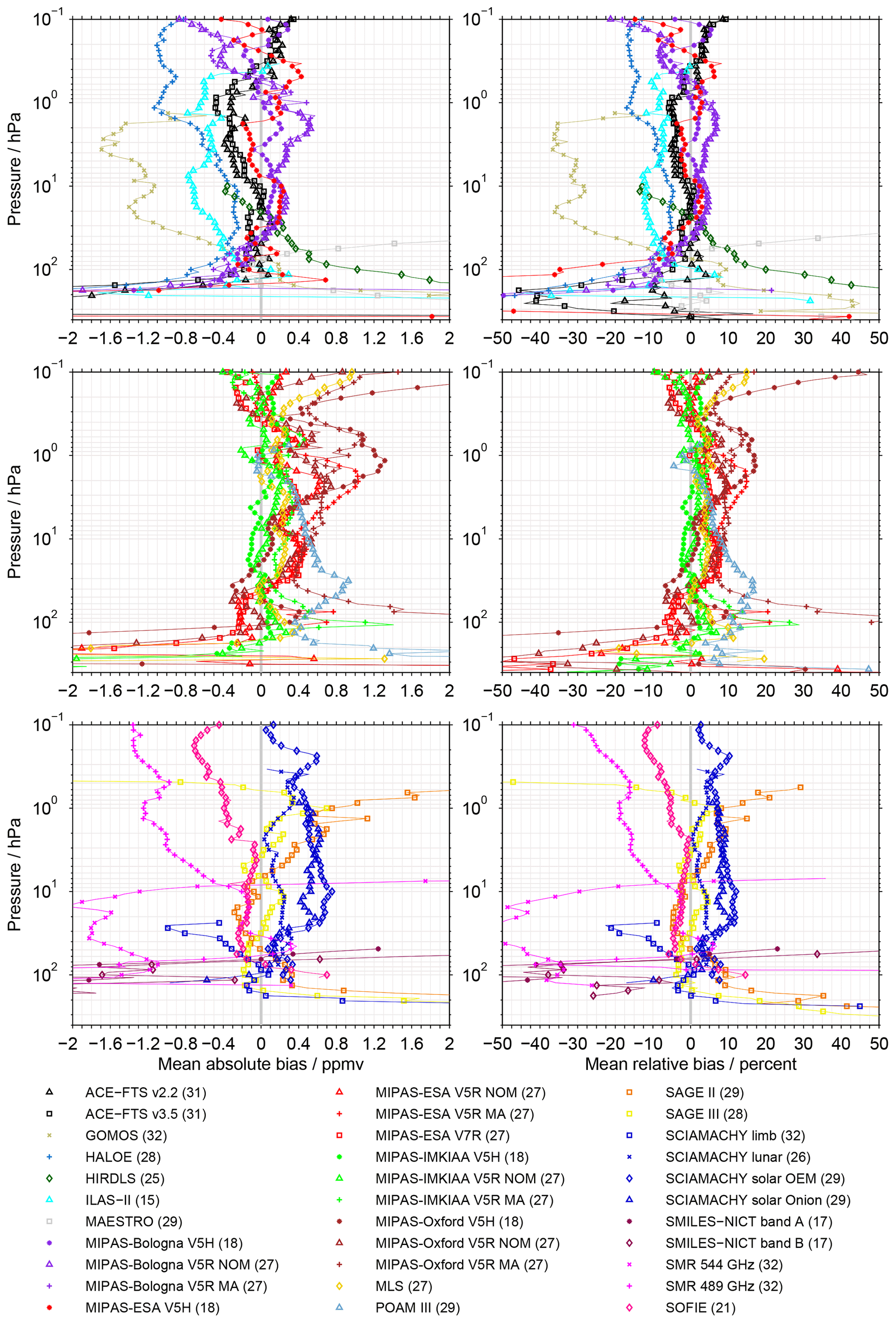
Figure 8A bias summary for all data sets. This summary is based on the comparisons that considers coincidences during all seasons and at all latitudes and takes into account the aggregation of the MIPAS results (see Sect. 3.5). Absolute biases are shown in the left column, relative biases in the right column. For the sake of better visibility the results have been split among three rows. The separation is also reflected by the legend columns. In the legend the number of comparisons contributing to the summary for the individual data sets is also indicated.
Finally, we want to note that the consideration of differences in the vertical resolution among the data sets, as done in this work (see Sect. 3.2), yields an improvement of the biases in 55 % of the comparisons (all data sets, times, latitude bands and altitudes). This primarily concerns altitudes above 70 hPa, and pronounced improvements are visible around 30 hPa in the stratopause and above 0.2 hPa. They can reach several tenths of a ppmv (or a few percent) in these altitude regions. Below 70 hPa there are both improvements and deteriorations, but with a clear tendency to the latter and as large as 100 % in relative terms. This indicates that differences in the vertical resolution are not the primary cause of the pronounced biases in this altitude region.
4.3 Data-set-specific results
In this section an overview of data-set-specific results is presented. Figure 8 shows the summary biases for all data sets, based on the comparisons that consider coincidences during all seasons and at all latitudes. The absolute biases are given in the left column and the relative biases in the right column. For the sake of better visibility the results have been split into three panels. In the legend this separation is also reflected by the columns. In addition, the legend contains the information on the number of comparisons contributing to the individual summary biases (using the aggregation of the MIPAS results). As described in Sect. 3.5 these results consider the aggregation of the MIPAS results. Overall the smallest biases are observed in the middle and upper stratosphere. The largest biases occur below 100 hPa (larger than ±2 ppmv or ±50 %). On occasion pronounced summary biases are also visible in the lower mesosphere close to 0.1 hPa.
The first row comprises the results for the ACE-FTS, GOMOS, HALOE, HIRDLS, ILAS-II, MAESTRO and some MIPAS data sets (Bologna and one from ESA). Here, the biases are relatively small with ±0.4 ppmv, corresponding to relative biases of ±10 %. Larger (negative) biases are found for the GOMOS, HALOE (above 2 hPa) and ILAS-II data sets. Among them, the GOMOS data set shows the absolute largest biases. The GOMOS biases get more negative with increasing altitude above 75 hPa and reach values of −1.4 ppmv at 20 hPa. Up to 2 hPa the biases of the GOMOS data set vary between −1.7 and −1.1 ppmv (roughly −35 % to −25 %). Above 2 hPa the biases decrease again in size; however this is close to the upper limit at which water vapour information can be retrieved from the GOMOS observations. The biases for the ILAS-II data set generally do not exceed −0.8 ppmv, corresponding to less than −15 % in relative terms. For the HALOE data sets the biases vary between −0.5 and −0.2 ppmv (−5 % to −10 %) in the altitude range from 70 to 5 hPa. Towards the lower mesosphere the biases increase in size, where they are around −1 ppmv (−15 %). At 0.1 hPa the biases for the data sets shown in the first panel range from −0.9 (−20 %) to 0.4 ppmv (10 %). Below 100 hPa the absolute biases increase significantly in size. All data sets exhibit biases larger than ±2 ppmv at some altitude. Also, in relative terms, a large variation is observed; however the biases for ACE-FTS v2.2 and MAESTRO data sets remain largely within ±10 %.
In the second panel results for numerous MIPAS (ESA, IMKIAA and Oxford) data sets are shown, plus those from the MLS and POAM III data sets. For these data sets the biases are generally within −0.3 to 0.6 ppmv, corresponding roughly to relative biases between −5 % and 10 %. Larger biases are found for the MIPAS-ESA V5R MA, MIPAS-Oxford V5H and MIPAS-Oxford V5R MA data sets around the stratopause. Some data sets exhibit a pronounced increase in their biases above 0.3 hPa. This concerns the MIPAS-Oxford and the MLS data sets. At 0.1 hPa biases range, overall, from −0.4 to more than 2 ppmv, corresponding to relative biases of −10 % to 45 %. Below 100 hPa again large biases are visible, with a tendency towards negative values. Data sets for which the biases exceed −50 % below 100 hPa are MIPAS-ESA V7R, MIPAS-Oxford V5H and MIPAS-Oxford V5R NOM. The MIPAS-ESA V5R NOM (−25 % to 0 %), MIPAS-IMKIAA (−20 % to 5 %), MLS (±20 %) and POAM II (5 % to 15 %) data sets show typically smaller biases here.
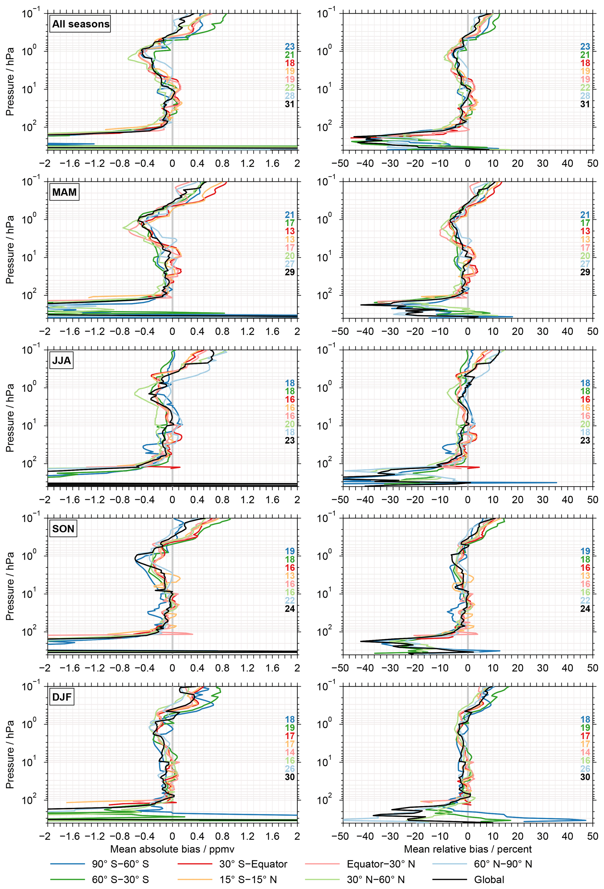
Figure 9Bias summary for the ACE-FTS v3.5 data set. The left column considers the absolute biases and the right column the relative biases. As in Figs. 6 and 7 the different rows focus on the results for different seasons or their combination. In the individual panels on the right the number of comparisons contributing to the summary are indicated. As described in Sect. 3.5 the number of comparisons to the different MIPAS data sets are counted individually, even though these results are aggregated.
The third panel of Fig. 8 presents results for data sets from the following instruments: SAGE, SCIAMACHY, SMILES, SMR and SOFIE. Here, some data sets exhibit quite pronounced biases. This concerns, on one hand, the experimental SMILES data sets. They cover the altitude range from slightly above 200 to 50 hPa and show good agreement between 70 and 60 hPa. Higher up, distinct positive biases (exceeding 1 ppmv or 20 %) are observed, while below negative biases of even larger size are visible. The summary biases for the SMR 544 GHz data set are almost entirely negative. Around 30 hPa they amount to −1.8 ppmv (exceeding −50 %). Above 15 hPa they get significantly smaller and switch sign at above 10 hPa, close to the upper limit of this data set. The biases for the SMR 489 GHz data set are quite low up to 10 hPa but start to increase significantly higher up. In the lower mesosphere this data set exhibits biases around −1.2 ppmv in absolute terms and −25 % in relative terms. In the lower half of the stratosphere the SAGE II, SAGE III, SCIAMACHY lunar and SOFIE data sets show very good agreement (typically within ±0.2 ppmv or ±5 %). Towards higher altitudes, biases increases to some extent, most prominently for the SAGE II data set above 3 hPa. The SCIAMACHY solar occultation data sets exhibit low biases in the lower stratosphere (around 5 %). Above 30 hPa they vary typically between 0.3 and 0.7 ppmv (5 % to 12 %).
Figure 9 shows the summary biases for the ACE-FTS v3.5 data set as a function of season and latitude, using the same layout as in Figs. 6 and 7. For all other data sets the corresponding figures are provided in the Supplement (Fig. S9). The comparisons to the ACE-FTS v3.5 data set show a rather consistent picture above about 100 hPa with relatively small variations among the different seasons and latitude bands. Between about 80 and 5 hPa the biases are typically within ±0.2 ppmv or ±5 %, with a clear preference towards negative biases. Towards higher altitudes the biases get more negative. They peak between 2 and 1 hPa with values from −0.8 (−10 %) to −0.2 ppmv (−2 %), depending on season and latitude. Above 1 hPa, the biases decrease again and switch sign at around 0.4 to 0.3 hPa. At 0.1 hPa there is a larger bias variation with season and latitude band. Here, the biases range between 0 and 0.9 ppmv (0 % to 15 %). Below 100 hPa a wide range of biases is observed, occasionally exceeding ±2 ppmv. The vast majority of the biases are negative. In relative terms they vary roughly between −40 % and 10 %.
For the presentation of the drift results we choose a similar approach as for the bias results. First, an example is shown, followed by a general assessment of the drifts in the observational database. After that, we present data-set-specific drift results. Finally, we compare the drift results with those obtained from the comparisons of monthly zonal mean time series presented in the work by Khosrawi et al. (2018). This aims to quantify how dependent the drift results are on the actual method to derive them.
As for the biases, the lower triangle of Fig. 2 provides an overview for which data set combinations drift comparisons were possible for any of the time–latitude bins considered in this work. In this context the yellow colour means that the overlap criterion of at least 36 months was not met and thus the drift results were not considered any further (see Sect 3.4). The overlap periods among the different data sets are shown in the lower triangle of Fig. 3. These numbers are based on the comparisons considering coincidences during all seasons and at all latitudes, maximising these periods. The longest overlap period is found between the two SMR data sets and amounts to 153 months. The comparisons of the SMR data sets with the ACE-FTS v3.5, MAESTRO and MLS data sets yield overlap periods beyond 120 months. The same is true for the comparisons of the ACE-FTS v3.5 data set to the MAESTRO and MLS data sets. Contrary, overlap periods of less than 40 months are, on one hand, found in the comparisons with the HIRDLS data set, which itself only comprises 39 months of data. On the other hand, the following comparisons have overlap periods between 36 months and 39 months: GOMOS vs. HALOE, GOMOS vs. SCIAMACHY lunar, HALOE vs. SCIAMACHY limb, POAM III vs. SCIAMACHY solar occultation, SAGE II vs. SCIAMACHY limb and SAGE III vs. SCIAMACHY limb.
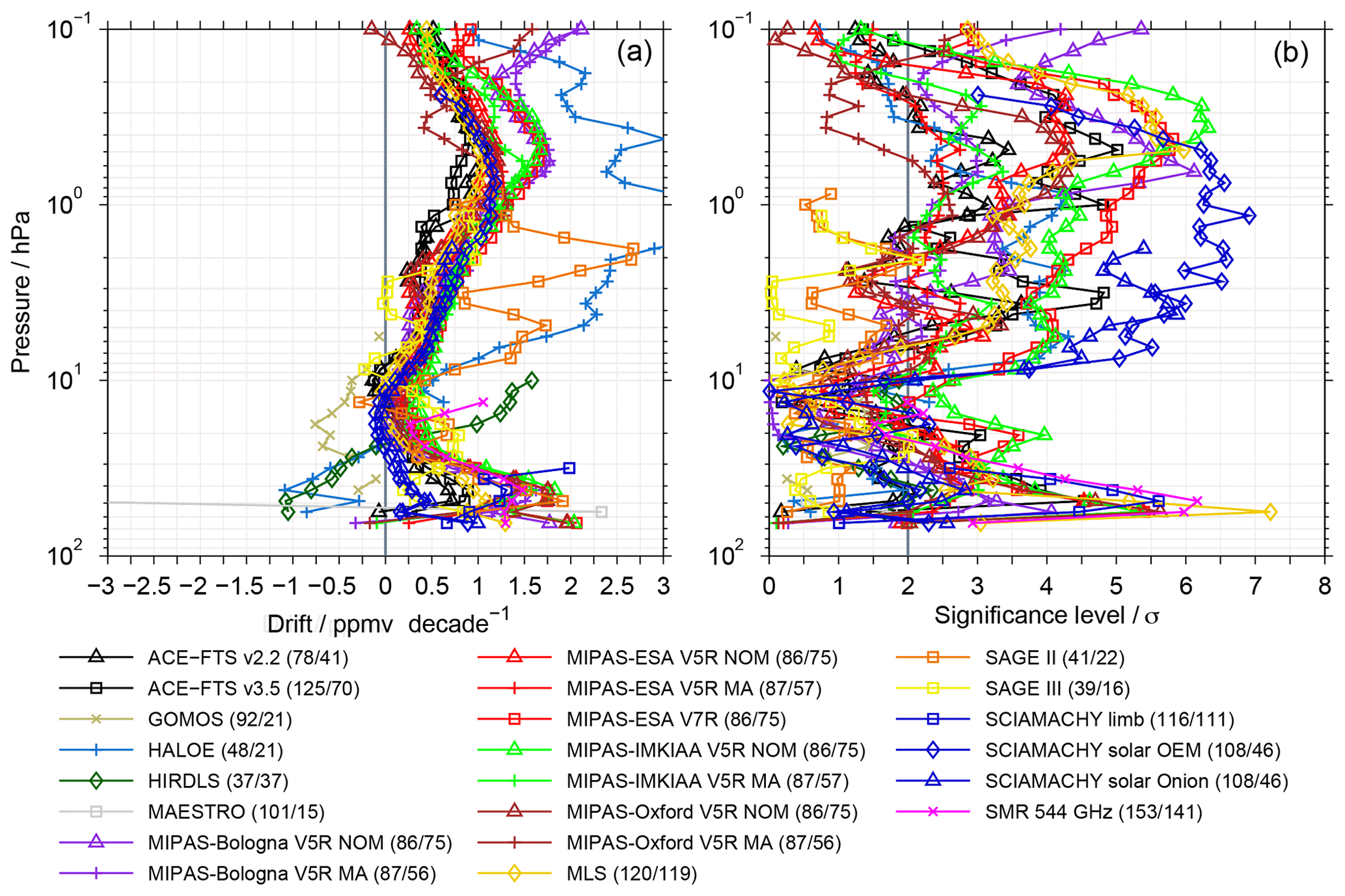
Figure 10Panel (a) shows the drift of the SMR 489 GHz data set relative to other data sets. In (b) the corresponding significance level of the drift estimates are shown. This example considers the latitude band between 30 and 60 ∘ N. In the legend the first number indicates the maximum overlap period in terms of months (over all altitudes) of the two data sets compared, i.e. the time between the first and the last month sufficient coincidences were found between the two data sets. The second number indicates during how many months both data sets actually yield sufficient coincidences, again represented by the maximum over all altitudes. As in Fig. 4 only results at every second altitude are plotted for better visibility.
5.1 Example
As an example we consider the drift of the SMR 489 GHz data relative to other data sets in the latitude range from 30 to 60∘ N. The drift estimates are shown in Fig. 10a. Fig. 10b shows the corresponding significance levels, defined as the absolute ratio between the drift estimates and their associated uncertainties (see Eq. 10). In the legend, for every data set, two numbers are provided. The first number indicates the overlap period of the two data sets in months. As described in Sect. 3.4, a minimum overlap period of 36 months was required for a drift to be calculated. The second number shows during how many months the two data sets actually have a sufficient number of coincidences. Since this information is altitude dependent, the legend considers the maximum values over all altitudes. The example indicates mostly positive drifts for the SMR 489 GHz data set, which means that its trends in water vapour are more positive or less negative than the trend estimates derived from the other data sets. The drifts are clearly systematic. Even though the comparisons consider different time periods, and thus the estimates can vary, a very consistent picture of their altitude dependence is obtained. Pronounced drifts are observed around 50 hPa, which is close to the lower altitude limit where water vapour retrievals from SMR observations are possible. The drifts are as large as 2 ppmv decade−1 and many of those are also statistically significant at the 2σ uncertainty level. Towards 20 hPa the drift estimates decrease to values smaller than 0.5 ppmv decade−1. The comparisons with a few data sets even indicate negative drift estimates for the SMR 489 GHz data set. Above 20 hPa, the drifts increase again and maximise at around 0.5 hPa. Here, the drift estimates typically range from 1 to 1.75 ppmv decade−1 and are in most cases statistically significant. Exceptions are the HALOE and SAGE II data sets, for which drift estimates are even larger than 2 ppmv. Above 0.5 hPa the drift estimates generally decrease again.

Figure 11Drift results for the full matrix of comparisons considering coincident observations during all seasons and at all latitudes. Drifts that are statistically significant at the 2σ uncertainty level are marked in light blue. Panel (a) shows the picture without the aggregation of the MIPAS results, while (b) considers this aggregation.
5.2 General results
Figure 11 shows the drift estimates from the full matrix of comparisons, similarly to the bias results shown in Fig. 5. Again, these results consider the comparisons that incorporate coincidences during all seasons and at all latitudes. The upper panel shows the picture without the aggregation of the MIPAS results. The picture in the lower panel takes this aggregation into account. Overall, from the 862 comparisons (see Sect. 4.2) in the full matrix, 470 comparisons yield drift results (see Fig. 2), with the chosen minimum overlap period of 36 months. In 450 comparisons drift estimates that are statistically significant at the 2σ uncertainty level are found. The estimates that are significant are marked in light blue in the figure. The picture without the aggregation of the MIPAS results indicates a wide range of drifts, in particular below 30 and at 0.1 hPa. Some of the extreme values can be assigned to specific data sets. Between 30 and 10 hPa the envelope of the drifts is smallest. Here, they are generally within ±0.4 ppmv decade−1. Also, based on the median, in this altitude range the smallest drifts are observed. Beyond that, we find that there is some dependence between the overlap period and the absolute drift size. Based on results above 100 hPa, the drift size typically decreases with increasing overlap period for periods up to 70 months. Beyond that overlap period, there is no obvious connection.
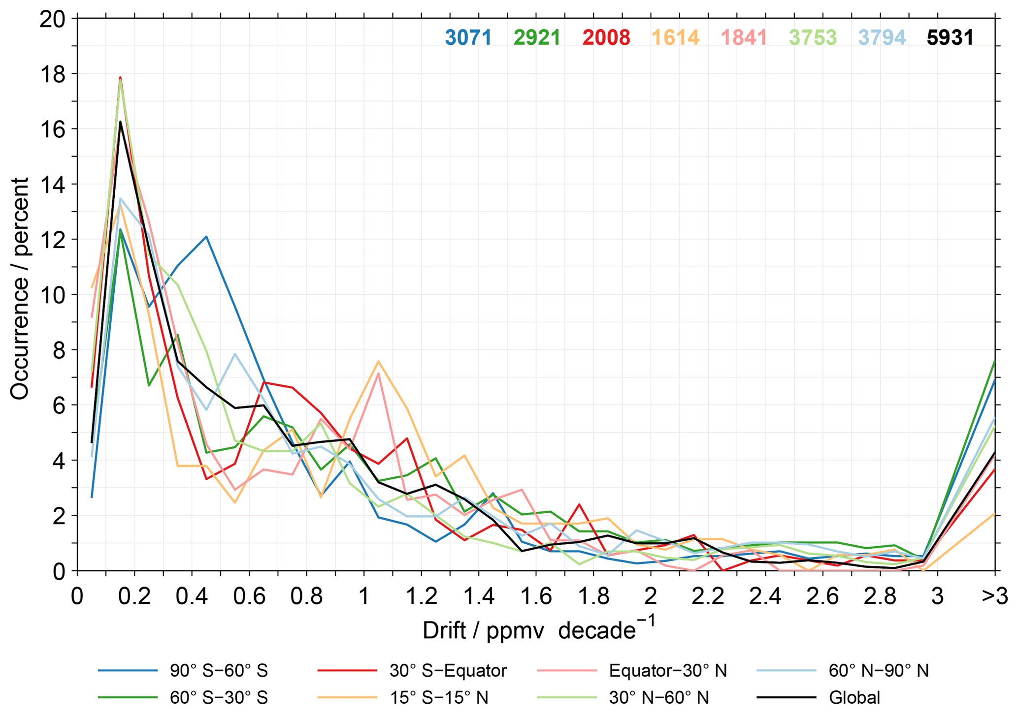
Figure 12Drift histograms using estimates from all altitudes and taking into account the aggregation of the MIPAS results. Only positive drifts and those that are statistically significant at the 2σ uncertainty level are considered in the calculation. The results for the different latitude bands are given by the different colours. In the upper-right corner the number of available data points is indicated, counting comparisons to different MIPAS data sets individually.
The picture with the aggregation of the MIPAS results is clearly sparser than that without the aggregation. Most prominently this is visible in the lower mesosphere, similarly to the corresponding picture for the biases shown in Fig. 5. In contrast to the unaggregated picture, a notable widening of the drift range at 0.1 hPa is not observed. At lower altitudes the picture is rather similar and the envelope of drifts exhibits a similar minimum region in the middle stratosphere. The typical drift sizes (based on the median) are typically larger for the picture with the aggregation of the MIPAS results, except above 0.2 hPa. Below 30 hPa the difference is of the order of 0.3 ppmv decade−1. Above 20 hPa the difference is roughly 0.1 ppmv decade−1.
In Fig. 12 drift histograms are shown for the different latitude bands, taking into account the aggregation of the MIPAS results. They consider the positive estimates from all altitudes that are statistically significant at the 2σ uncertainty level. In the upper-right corner of the figure the number of available data points is indicated. Bins of 0.1 ppmv decade−1 are used for the histograms. The smallest drifts have the lowest occurrence rate in the Antarctic (about 2.5 %) and Arctic (4 %). In contrast, the largest occurrence rates are observed in the latitude bands from the Equator to 30∘ N (9.25 %) and from 15∘ S to 15∘ N (10.25 %). Beyond the smallest drift bin, the occurrence rates quickly rise. In fact, the maximum occurrence rates are observed for drifts between 0.1 and 0.2 ppmv decade−1, consistently for all latitude bands. They vary between 12.25 % (60 to 30∘ S and Antarctic) and 18 % (30∘ S to Equator and 30 to 60∘ N). Towards larger drifts the occurrence rates generally decrease. However, there are some prominent additional maxima, for example in the Antarctic for drifts between 0.4 and 0.5 ppmv decade−1 (occurrence rate of 12 %). For drifts of 1 ppmv decade−1 the occurrence rate is between 2.75 % and 4.25 %, except for the latitude bands from 15∘ S to 15∘ N and from the Equator to 30∘ N. In those latitude bands again pronounced additional maximum in the occurrence rate (7 % to 7.5 % for the bin between 1.0 and 1.1 ppmv decade−1) are visible. For drifts of 2 ppmv decade−1 the occurrence rate is smaller than 1.5 % and minimises for the Antarctic. Drifts larger 3 ppmv decade−1 occur in 2 % to 7.5 % of the comparisons with the highest occurrence rate for the latitude band from 60 to 30∘ S and the lowest occurrence rate for the latitude band between 15∘ S and 15∘ N.
In the Supplement, in Fig. S10, the corresponding picture without the aggregation of the MIPAS results is shown. In contrast to Fig. 12, the maximum occurrence rates are larger (between 14.5 % and 19.25 %). Prominently, the maximum occurrence rate in the Antarctic is found first for drifts between 0.3 and 0.4 ppmv decade−1. Also, for the latitude band from 30 to 60∘ N and the Arctic, the maximum occurrence rate is observed at larger drifts than for the aggregated results. Note that secondary maxima in the occurrence rate are not visible in the results without the MIPAS aggregation. The occurrence rates for drifts larger than 1 ppmv decade−1 are on average smaller than for the picture with the aggregation of the MIPAS results. Also, the variation with increasing drifts and among the latitude bands is smaller in Fig. S10.
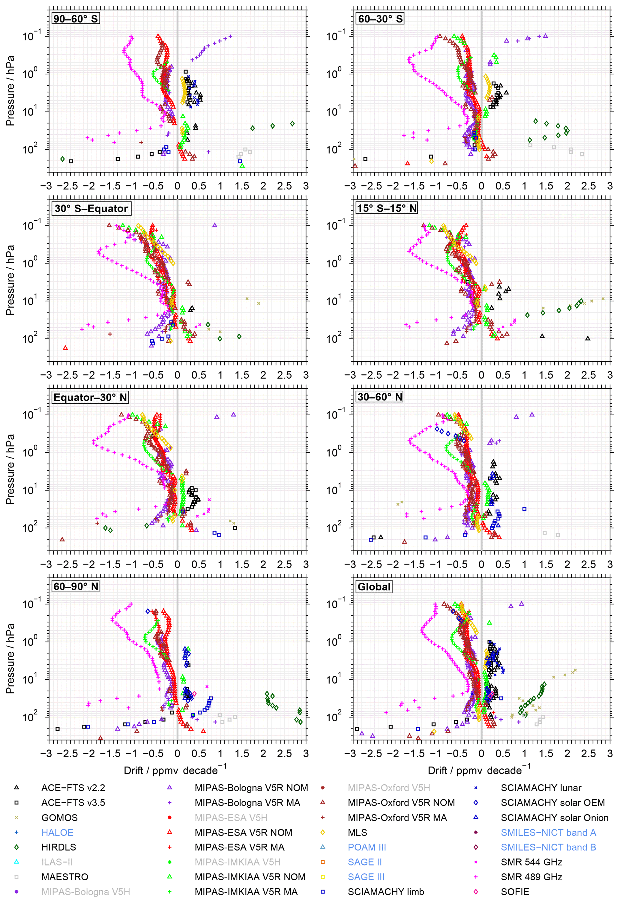
Figure 13Drift summary for the MIPAS-ESA v7 data set. The summary shows only drifts that are statistically significant at the 2σ uncertainty level and only results at every second altitude are plotted (as in Figs. 4 and 10). The different panels consider the results for different latitude bands. The legend lists all possible data sets. Whether they contribute results or not is indicated by different colours, as described in Sect. 5.3.
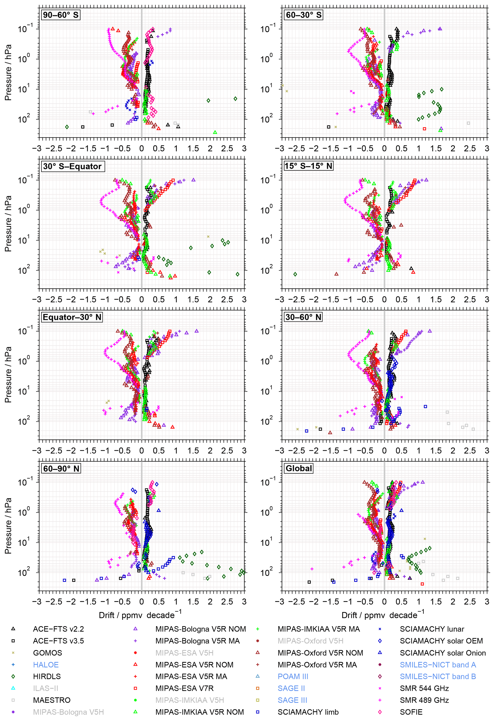
5.3 Data-set-specific results
In this section we provide a summary of data-set-specific drift results, focusing on the MIPAS-ESA V7R (Fig. 13) and the MLS data sets (Fig. 14). All remaining results can be found in Fig. S11 in the Supplement. No results are available for the ILAS-II, MIPAS V5H and SMILES data sets. These cover a too-short time period for a drift analysis according to our criteria defined in Sect. 3.4. A summary figure for given data set shows all drifts that are statistically significant at the 2σ uncertainty level relative to this data set. For better distinction between the data sets, results are only plotted at every second altitude, i.e. with a sampling of ∼1 km (see Sect. 3.3 as well as Figs. 4 and 10). The different panels focus on different latitude bands, as indicated in the upper left. For some of the data sets (e.g. GOMOS, HALOE, POAM III; see the Supplement) there are occasionally no results for any of the latitude bands. In these cases there will be information explaining why, in accordance with the list below:
-
No comparisons. No comparisons to other data sets could be made due to missing overlap (at least 20 coincidences; see Sect. 3.3).
-
No drift data. Comparisons to other data sets were made but yielded no drift results. This is because the overlap period is too short or too few data points exist to derive drift estimates.
-
No significant results. Drifts were derived, but none of them are statistically significant at the 2σ uncertainty level.
-
Significant results only outside the plot range. Statistically significant drifts were derived, but those are outside the plot range from −3 to 3 ppmv decade−1. This is already a large range that covers of the vast majority of reasonable estimates.
In the legend all possible data sets are listed. Colour coding is used to convey extra information to which data sets may or may not contribute results (on a global scale):
-
Dark grey means no comparisons.
-
Light blue means no drift data.
-
Dark red means that significant results only exist outside the plot range. This occurs only in a few comparisons (e.g. in the comparison between the GOMOS and SOFIE data sets) and in these cases concerns just a handful of data points. In the figures shown here in the main paper no such case occurs.
-
Black means that the comparisons to these data sets yield drifts that are significant at the 2σ uncertainty level and, thus, these drift results are visible in the given summary figure.
The comparisons to the MIPAS-ESA V7R data set exhibit predominantly negative drifts as visible in Fig. 13. These negative drifts minimise in size, typically around 20 to 10 hPa (up to −0.3 to −0.4 ppmv decade−1), and increase towards lower and higher altitudes. Around 50 hPa large negative drifts (beyond −1 ppmv decade−1) are observed relative to the SMR 489 GHz data set in all latitude bands. Below 100 hPa drifts of similar size are found more frequently relative to a number of data sets. In the mesosphere the comparison to SMR 489 GHz data set again yields large negative drifts. They often peak in size around 0.5 hPa (in the polar regions a bit higher up) with values between −2 and −1.2 ppmv decade−1. At 0.1 hPa the negative drifts vary between −1.6 and −0.3 ppmv decade−1, based on the comparisons to the other MIPAS V5R NOM, MLS and SMR 489 GHz data sets. Notable positive drifts (beyond 1 ppmv decade−1) are found below 20 hPa relative to the HIRDLS, GOMOS, MAESTRO data sets at selected latitudes. Smaller positive drifts occur in the comparisons to the MIPAS V5R NOM data sets derived with the Bologna, IMKIAA and Oxford processors as well as some SCIAMACHY data sets. In the latitude bands from 90 to 60∘ S and 60 to 30∘ S, drifts up to 0.5 ppmv decade−1 are observed in the altitude range from 8 to 1 hPa in the comparisons with the ACE-FTS, MLS and SCIAMACHY lunar (only Antarctic) data sets. Close to 0.1 hPa pronounced positive drifts are often found relative to the any of MIPAS-Bologna data sets (except in the latitude from 15∘ S to 15∘ N and 60 to 90∘ N).
The MIPAS V5 data sets are prone to a small drift since the correction coefficients for the non-linearity in the detector response function have changed over time and this is not accounted for in the V5 calibration (Walker and Stiller, 2019). In the MIPAS V7 calibration a time dependence of these coefficients is considered and, thus, data sets derived from this calibration are expected to show fewer drifts. Compared with its predecessor data set, i.e. MIPAS-ESA V5R NOM, the MIPAS-ESA V7R data set indeed exhibits a reduced number of significant drifts. Considering the comparisons with non-MIPAS data sets, the number is reduced by 4.6 %. If only comparisons with the ACE-FTS v3.5 and MLS data sets are taken into consideration, the reduction amounts to 25 %. In contrast to the MIPAS-ESA V7R data set, the MIPAS-ESA V5R NOM data set shows a predominance of positive drifts (see Fig. S11 in the Supplement). This might be a hint that the correction coefficients used in the MIPAS V7 calibration overcompensate for the original issue in the V5 calibration.
The comparisons with the MLS data set (Fig. 14) yield both negative and positive drifts with a slight prevalence of the former. Typically the drift estimates are within ±0.5 ppmv decade−1. Larger drifts are prominently found in the comparisons with the GOMOS (negative), HIRDLS (primarily positive) and SMR 489 GHz data sets, which highlight issues with these data sets rather than with the MLS data set itself. Positive drifts are consistently found relative to the ACE-FTS data set (around 0.2 ppmv decade−1). A similar picture is observed in the comparisons with the SCIAMACHY solar occultation data sets. In the lower stratosphere the comparisons with the MIPAS-ESA V5R NOM (roughly up to about 60 hPa), MIPAS-IMKIAA V5R NOM (up to about 10 hPa) and MIPAS-Oxford V5R NOM (up to about 30 to 20 hPa) exhibit positive drift estimates. In the lower mesosphere the drifts are positive relative to the MIPAS-Bologna, MIPAS-ESA V7R (not in the Antarctic and from 60 to 30∘ S) and the MIPAS-IMKIAA V5R NOM (except in the Antarctic) data sets. In addition, the comparisons with the SOFIE data set indicate positive drifts in the Antarctic (with a gap between 9 and 1.5 hPa) and the Arctic lower mesosphere. In contrast, negative drifts are found relative to the MIPAS-Bologna data sets below about 1 hPa, the MIPAS-ESA data sets (except those positive drifts mentioned before), the V5R MA data sets derived with the IMKIAA and Oxford processors, the MIPAS-Oxford V5R NOM data set above about 30 to 20 hPa as well as the SMR 489 GHz data set.
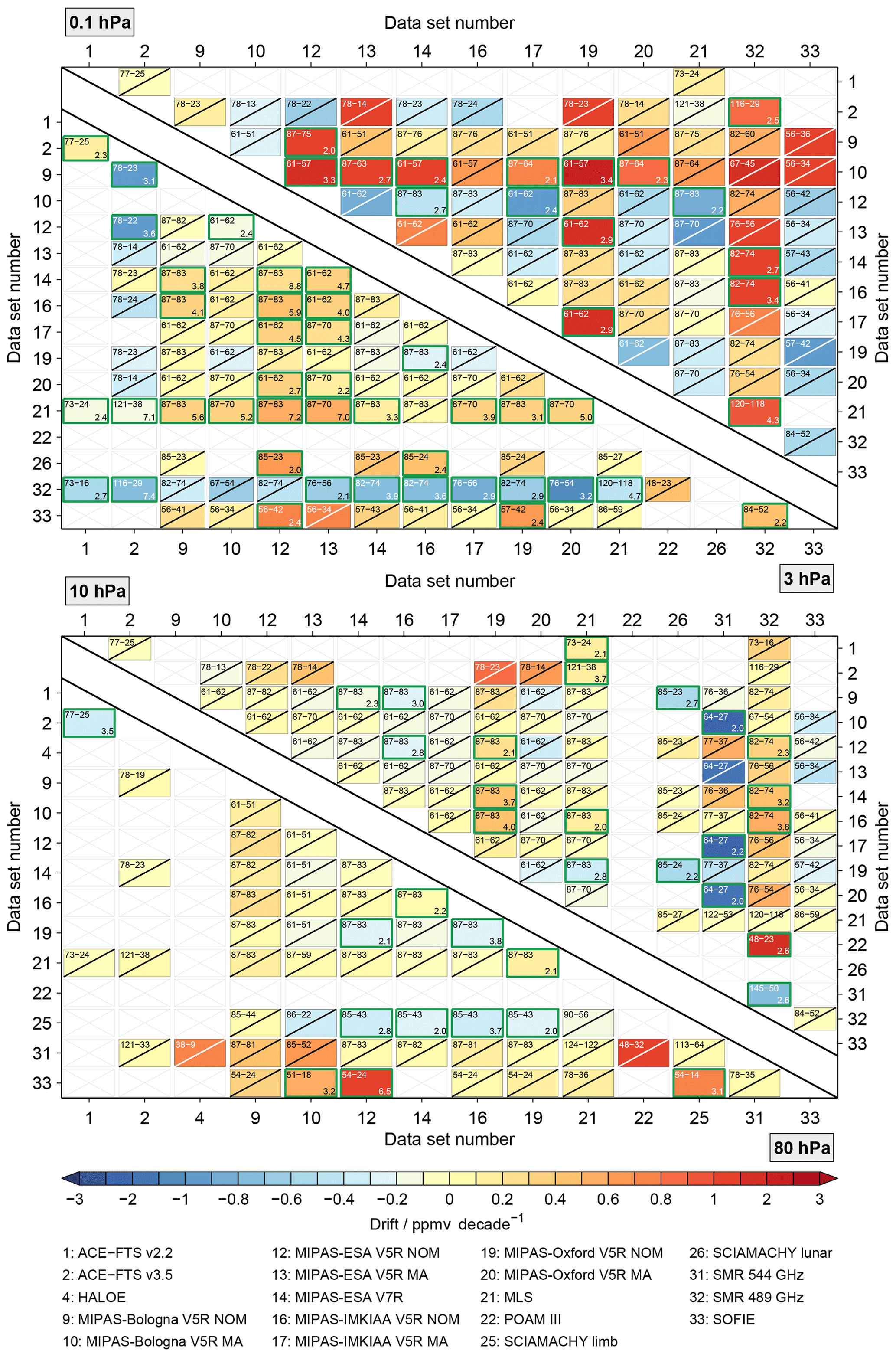
Figure 15Drifts between the different data sets in the latitude band between 80 and 70∘ S at 80, 10, 3 and 0.1 hPa. The drift estimates are based on the difference time series between the data sets given at the x axis and the data sets given at the y axis. Data sets are only shown if they yield any result at a given altitude. Besides the colour-coded drift estimates the result boxes contain additional information. In the upper left, the overlap period of the two data sets is given first. The second number indicates how many months the data sets actually overlap. If a drift is not significant at the 2σ uncertainty level this is marked by a slant. In contrast, if a drift is significant this is marked by a green frame and the significance level is noted in the lower-right corner.
5.4 Method comparison
In this work we present drift results based on coincident observations. In a preceding WAVAS-II work we presented drift estimates among the different data sets based on the comparison of their zonal mean time series (Khosrawi et al., 2018). The latter approach has the advantage that more data can be used, typically also allowing more comparisons. The disadvantage of the zonal mean time series approach is that it is more prone to sampling errors (in time and space) and does not take into account differences in vertical resolution among the data sets, which, under circumstances, may influence the drift estimates. Here, we want to compare the results from these two comparison methods and assess how often the drift estimates differ or not. For that, Fig. 15 shows the drift estimates among the different data sets, calculated using the profile-to-profile method, in a matrix form considering data in the latitude band from 80 to 70∘ S at 80, 10, 3 and 0.1 hPa (from top to bottom). The drift estimates are based on the difference time series between the data sets given at the x axis and the data sets given at the y axis. Data sets are only shown if they yield any result at a given altitude to optimise the available space. The drift estimates are colour coded. In addition to that, different types of auxiliary information are provided in the result boxes. In the upper left, the overlap period of the two data sets is given as well as the number of months the data sets actually overlap. A non-significant drift (at the 2σ uncertainty level) is indicated by a slant. For contrast a significant drift is marked by a green frame and the significance level is noted in the lower-right corner. As such the figure is directly comparable with Fig. 11, shown in the work of Khosrawi et al. (2018). Both figures exhibit a number of similar patterns. At 0.1 hPa the drift size is the largest among the four altitudes with prominent examples in the comparisons relative to the MIPAS-Bologna V5R MA and SMR 489 GHz data sets. At 3 hPa the large drifts relative to SMR 489 GHz are again a common feature among the two drift estimation methods. Smaller drift sizes are observed both at 10 and 80 hPa with exceptions attributed to the same data sets.
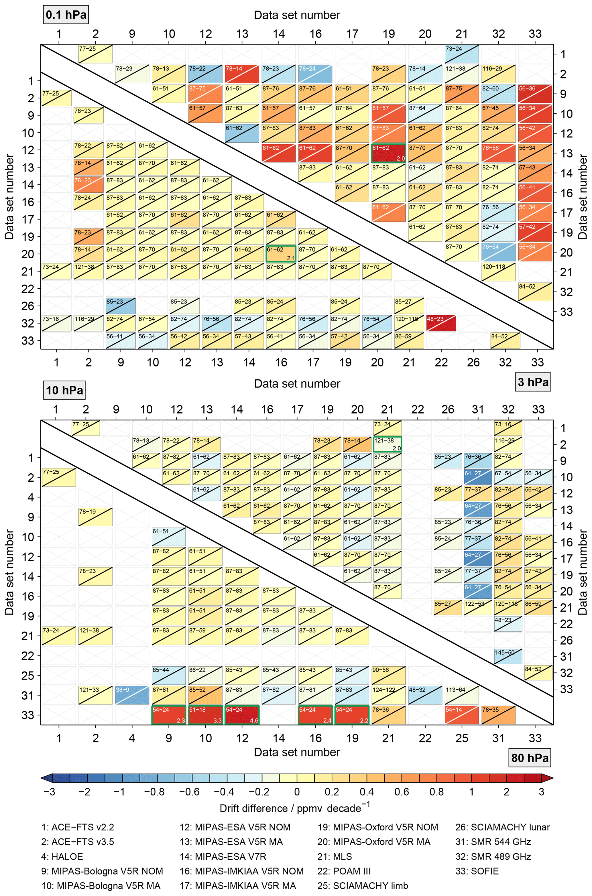
Figure 16As in Fig. 15, but here the differences between the drift estimates derived from the profile-to-profile comparisons and those obtained from the comparisons of zonal mean time series (see Eq. 13) are shown. The characteristic numbers in the result boxes correspond to the profile-to-profile comparisons. Typically they are not the same for the comparisons of zonal mean time series and, thus, are just displayed for guidance. Differences not statistically significant at the 2σ uncertainty level (see Eq. 14) are marked by a slant; otherwise the significance level is again indicated in the lower-right corner.
For a more quantitative comparison, Fig. 16 shows the actual drift differences ΔCdrift between the two approaches, i.e.
in the same style as Fig. 15. Here, represents the drifts derived from the profile-to-profile comparisons (this work) and the drifts based on the comparisons of the zonal mean time series (Khosrawi et al., 2018). The uncertainty of this difference εdrift is given by
where and are the drift uncertainties from the two approaches and any covariance among them is neglected. The characteristic numbers in the result boxes of Fig. 16 correspond to the profile-to-profile comparisons. Differences not statistically significant at the 2σ uncertainty level are again marked by a slant, while for significant differences the significance level is once more provided in the lower-right corner. The largest differences between the drift estimates from the two approaches occur at 0.1 hPa and amount to 0.4 ppmv decade−1 on average. Prominent examples are visible in comparisons with the ACE-FTS v3.5, SMR 489 GHz and SOFIE data sets. Also, some comparisons among MIPAS data sets exhibit large differences in the drift estimates. In contrast, at 3 hPa the drift differences minimise among the four altitudes shown in Fig. 16 (on average 0.15 ppmv decade−1). Also, at 10 and 80 hPa, relatively small differences in the drift estimates from the two approaches are found. A few noteworthy exceptions occur in comparisons with the SMR 544 GHz and SOFIE data sets. Even though the drift estimates derived from the profile-to-profile and zonal mean time series comparisons occasionally exhibit larger differences, they are only statistically significant (at the 2σ uncertainty level) in 2.6 % of the comparisons shown in Fig. 16.
In addition, the zonal mean time series comparisons presented by Khosrawi et al. (2018) consider the latitude bands from 15∘ S to 15∘ N and from 50 to 60∘ N. For these latitude bands the figures corresponding to Figs. 15 and 16 are shown in the Supplement (see Figs. S12, S13 and S14, S15). In summary, for the tropical band, the drift differences maximise on average at 80 hPa, close the top of the highly variable tropical tropopause layer. The minimum differences are observed at 3 hPa for the latitude band from 80 to 70∘ S. In total, in 6.0 % of the comparisons, the drift estimates from the two approaches differ significantly. For the latitude band from 50 to 60∘ N the differences are largest at 0.1 hPa and smallest at 3 hPa. In 3.8 % of the comparisons the drift differences are significant at the 2σ uncertainty level in this latitude band.
For the eight latitude bands primarily considered in this work and altitudes above 100 hPa, overall, in 3.2 % of the comparisons the drift estimates derived with the profile-to-profile and zonal mean time series comparisons differ at the 2σ uncertainty level. On average, the differences in the drift estimates are largest for comparisons among occultation data sets (i.e. ACE-FTS, GOMOS, HALOE MAESTRO, POAM, SAGE, SCIAMACHY occultation and SOFIE). For the remaining data sets with more dense temporal and spatial sampling (i.e. HIRDLS, MIPAS, MLS, SCIAMACHY limb, SMR) the differences are clearly smaller. At the same time the percentage of significant differences in the drift estimates is smallest for comparisons between the occultation data sets and largest for comparisons between more dense data sets. Comparisons between occultation and more dense data sets yield statistics in the middle.
Overall, the differences in the drift estimates from the two approaches minimise in the altitude range between 5 and 2 hPa (typically, based on the median, between 0.05 and 0.1 ppmv decade−1). The largest differences are observed towards 100 and 0.1 hPa (typically beyond 0.15 ppmv decade−1 median-wise). For individual comparisons the differences between the drift estimates derived with the profile-to-profile and zonal mean time series comparisons can be significantly larger, as visible in the example shown in Fig. 16.
In this work, biases and drifts among 33 data sets of stratospheric and lower mesospheric water vapour, from 15 different satellite instruments, were assessed using profile-to-profile comparisons. In terms of biases, both absolute and relative estimates were considered. For the relative estimates the mean of the data sets that were compared was used as reference (see Sect. 3.3).
Typically, the observational database exhibits the largest biases below 70 hPa, both in absolute and relative terms (see Figs. 5 and 6). In contrast, the lowest biases are generally observed between 70 and 5 hPa. Based on the 50 % percentile (median) over the different comparison results, the typical biases vary between 0.25 and 0.5 ppmv (5 % to 10 %) in this altitude region. The smallest biases occur here at low latitudes and midlatitudes. Higher up, the biases generally increase accompanied by considerable variations with altitude and latitude band. Typical bias values range from 0.3 to 1 ppmv (4 % to 20 %), again based on the 50 % percentile. Histograms considering comparison results from all altitudes show the largest occurrence rates for biases up to 0.2 ppmv or 5 % (see Fig. 7). For other altitude regions (see Figs. S6 to S8) this behaviour is not is always found, most prominently in the altitude range from 10 to 1 hPa. There is no simple picture of which latitude band yields the highest (lowest) occurrences for low (high) biases and vice versa.
Besides a general assessment of the biases in the observational database we also focused on data-set-specific issues in our work (see Figs. 8, 9 and S9). This analysis was based on bias summaries which combined the comparison results of a specific data set to all other data sets (see Sect. 3.3), including an aggregation of the comparison results to the various MIPAS data sets (see Sect. 3.5). The most noteworthy data-set-specific biases are listed below:
-
For the ACE-FTS data sets some negative biases are found in the upper stratosphere. They roughly amount to up to −0.5 ppmv in absolute terms and to −10 % in relative terms.
-
The GOMOS data set shows clear negative biases (exceeding −1.5 ppmv) above 50 hPa with pronounced variations among the different latitude bands considered in this work as well as the season.
-
In the lower mesosphere the HALOE data set shows large negative biases of about −1 ppmv (−15 %).
-
The HIRDLS data set shows distinct positive biases around 100 hPa (roughly around 1 ppmv or 20 %). Towards the upper limit of this data set at 10 hPa its biases also show a pronounced latitudinal dependence.
-
In the middle and upper stratosphere the ILAS-II data set exhibits notable negative biases (around −0.8 ppmv).
-
For the MAESTRO data set the biases deteriorate at its upper end close to 40 hPa. Below, the biases in the tropics and subtropics exceed 1 ppmv (20 %) on many occasions.
-
The MIPAS-Bologna V5R data sets show more pronounced biases around 2 hPa (about 0.4 ppmv or 8 %). Close to 0.1 hPa the biases of all Bologna data sets are clearly negative in most seasons and latitude bands (often exceeding −1 ppmv or −25 %).
Similarly to the MIPAS-Bologna V5R data sets, the MIPAS-ESA V5R data sets exhibit notable positive biases (peaking roughly about 0.5 ppmv or 10 %) in the upper stratosphere. For the MIPAS-ESA V7R data set such biases are observed in the middle stratosphere. The MIPAS-ESA V5H data set shows distinct negative biases close to 0.1 hPa, as noted for the Bologna data sets.
The MIPAS-IMKIAA V5R NOM data set also exhibits distinct negative biases close to 0.1 hPa in numerous seasons and latitude bands (can be as large as −1 ppmv or −25 %). Such behaviour is also visible in the MIPAS-IMKIAA V5R MA data set but not as pronounced.
In the upper stratosphere and lower mesosphere the MIPAS-Oxford V5H data sets show substantial positive biases, with a pronounced seasonal and latitudinal variation. At 1 hPa the biases vary around 1 ppmv (15 %), while at 0.1 hPa they are clearly larger. Similarly to a number of MIPAS data sets, the MIPAS-Oxford V5H NOM data set exhibit notable positive biases in the upper stratosphere (also peaking roughly around 0.5 ppmv or 10 %). The MIPAS-Oxford V5R MA data set shows prominent positive biases at almost all latitudes. They roughly amount to around 0.5 ppmv (10 %), with larger estimates close to 0.1 hPa.
-
The biases for the MLS data set are mostly positive and typically smaller than 0.4 ppmv (roughly 8 %). Exceptions exist below 100 hPa and close to 0.1 hPa.
-
The POAM data set shows a distinct positive bias in the lower stratosphere (around 0.8 ppmv or 15 %).
-
Around 1 hPa the biases of the SAGE II data set are of the order of 1 ppmv (15 %).
-
Both SMILES data sets show large biases with both signs in the small altitude range where this data set provides coverage (slightly above 200 to 50 hPa).
-
The biases of the SCIAMACHY limb data set are clearly negative (roughly −15 %) at the upper end (about 30 hPa) and positive (roughly 25 %) at the lower end (somewhat below 200 %). The other three data sets derived from the SCIAMACHY observations exhibit mostly positive biases. These biases are most pronounced for the solar occultation data sets in the middle and upper stratosphere (around 0.5 ppmv or 10 %).
-
In the lower stratosphere the SMR 544 GHz data sets show pronounced negative biases, often in excess of −1.2 ppmv (−35 %). Similarly, the other SMR data set in this assessment, based on water vapour emissions at 489 GHz, exhibits notable negative biases in the upper stratosphere and lower mesosphere. These biases occasionally exceed −1 ppmv (−15 %).
-
In the uppermost stratosphere and lower mesosphere the SOFIE data set exhibits more pronounced biases, roughly around −0.5 ppmv or −8 %.
For the drift assessment we considered a minimum overlap period of 36 months for the data sets when comparing them with each other. Overall, the observational database shows a wide range of drifts that are statistically significant at the 2σ uncertainty level. In general, the smallest drifts are found between about 30 to 10 hPa. In this altitude region the drifts typically do not exceed 0.25 ppmv decade−1 (0.40 ppmv decade−1) for the aggregated (unaggregated) global comparisons (see Fig. 11). For other latitude bands the maximum drifts are slightly larger. Histograms considering statistically significant results from all altitudes indicate the largest occurrence for drifts between 0.1 and 0.2 ppmv decade−1.
While the comparison of two data sets does not immediately indicate which data set is responsible for any observed drift, comparisons with a multitude of data sets have the potential to obtain a clearer picture. In our analysis the data sets with the most prominent drifts are as follows:
-
GOMOS data set – primarily negative drifts
-
HIRDLS data set – negative drifts
-
MAESTRO data set – negative drifts
-
SMR 544 GHz and SMR 489 GHz data sets – positive drifts.
Other noteworthy results are as follows:
-
For the MIPAS V5 data sets a small drift has been expected (Walker and Stiller, 2019) and is also detected. This can be explained with the calibration of these data sets, which does not account for any time dependence of the correction coefficients for the non-linearity in the detector response. These data sets show primarily positive drifts in the stratosphere: the only exception is the IMKAA V5R NOM data set, which exhibits mostly negative drifts. The V7 calibration of the MIPAS data implements a time dependence of the correction coefficients. For the MIPAS-ESA V7R data set the number of significant drifts is indeed reduced compared with the MIPAS-ESA V5R NOM, which is the direct predecessor. The reduction is nearly 5 % for the comparisons with non-MIPAS data sets and 25 % for the comparisons with the ACE-FTS v3.5 and MLS data sets. The majority of drift estimates for the MIPAS-ESA V7R data set are, however, negative, in contrast to the predecessor data set. This might suggest that the new correction coefficients implemented in the MIPAS v7 calibration overcompensate the original drift issue. In general, the stratospheric drift estimates for the MIPAS data sets are roughly within ±0.5 ppmv decade−1.
-
Also, for the ACE-FTS, MLS, SCIAMACHY and SOFIE data sets, a drift range roughly within ±0.5 ppmv decade−1 can be reported. For the MLS data set almost an equivalence of positive and negative drifts is observed. The drift estimates for the data sets from the other three instruments are primarily negative.
-
For the HALOE, POAM III, SAGE II, SAGE III data sets only a limited drift assessment is possible. This is because there are only a few data sets which have sufficiently long overlap periods for a drift estimation. Among them are the SMR data sets that have their own issues. Beyond that there is not always consistency in the results which would provide more certainty towards any potential problem for these four data sets.
Finally, we compared our drift estimates with those derived from comparisons of zonal mean time series as presented by Khosrawi et al. (2018). Our profile-to-profile comparisons have the advantage that they minimise sampling errors among the data sets to be compared. Also, differences in the vertical resolution of the data sets can be taken into account. Comparisons of zonal mean time series typically allow more data to be included, potentially yielding more comparisons. In our analysis we found that the differences among the drift estimates from the two approaches are in general largest for comparisons among occultation data sets. For comparisons between data sets with more dense temporal and spatial sampling, the differences are on average smaller. However, the percentage of statistically significant (at the 2σ uncertainty level) differences is larger. For the three latitude bands (80–70∘ S, 15∘ S–15∘ N and 50–60∘ N) and four altitudes (80, 10, 3 and 0.1 hPa) considered in the work of Khosrawi et al. (2018), we found that only in 2.6 % to 6.0 % of the comparisons the drift estimates derived from the profile-to-profile and zonal mean time series comparisons differed significantly at the 2σ uncertainty level. For the eight latitude bands primarily considered in this work and for altitudes above 100 hPa, statistically significant drift differences occurred in 3.2 % of the comparisons. Hence, there is largely no need for a specific approach to derive the drift estimates.
In our work we consider 13 MIPAS data sets out of 33 data sets in total. Even though they are based on different measurement modes and processors with different retrieval choices, they exhibit some relative similarity with respect to the remaining data sets. This behaviour has obvious effects on our results and conclusions. Therefore, the general results and the bias summaries of the individual data sets presented in this work consider an aggregation of the results obtained from MIPAS data sets (see Sect. 3.5). With this aggregation the bias percentiles typically exhibit larger values and a smaller occurrence rate for the smallest biases is observed. In addition, the results vary more strongly among the different seasons and latitude bands.
Overall, we find that many data sets are useful for scientific analyses, either considering the observational data themselves or in connection with modelling results. For scientific studies where the absolute amount of water vapour is the key the data sets listed above with bias issues should be used with caution. Likewise, those data sets mentioned with drift issues should be treated with care if variability beyond 36 months is of interest. By combining the bias and drift characteristics found in this work, the altitude range between 50 and 5 hPa shows the fewest number of issues in the observational database, making it most optimal place for scientific analyses regarding stratospheric and lower mesospheric water vapour.
Results from WAVAS-II activity can be found on the following website: https://zenodo.org/communities/wavas-ii/.
In this work we considered the mean of the data sets as the reference for relative bias estimates (see Sect. 3.3). As described, any a posteriori attempt to relate the relative bias to the first or the second data set (instead of the mean) can lead to non-intuitive results. According to Eq. (8) the relation between the relative bias, the abundance of the first data set and the abundance of the second data set can be written as follows:
For a bias of −100 % the relation of the two data sets becomes
while for a bias of 100 % the relation is
These kind of relations should be kept in mind.
The supplement related to this article is available online at: https://doi.org/10.5194/amt-12-2693-2019-supplement.
The study was designed by the WAVAS-II core members JCG, DH, FK, MK, SL, GEN, WGR, KHR, GPS and KAW. Satellite data used in this study were provided by KAW, JLP, LB, JCG, TS, CES, BMD, EP, PR, MGC, AD, WGR, GEN, RPD, JMZ, KW, AR, FA, KB, SN, HS, YK, JU, PE and MEH. The data were processed and analysed by SL and MK. SL and FK wrote the manuscript. All co-authors helped with the interpretation and discussion of the results.
The authors declare that they have no conflict of interest.
This article is part of the special issue “Water vapour in the upper troposphere and middle atmosphere: a WCRP/SPARC satellite data quality assessment including biases, variability, and drifts (ACP/AMT/ESSD inter-journal SI)”. It is not associated with a conference.
The Atmospheric Chemistry Experiment (ACE), also known as SCISAT, is a
Canadian-led mission mainly supported by the Canadian Space Agency and the
Natural Sciences and Engineering Research Council of Canada. We appreciate
the HALOE Science Team and the many members of the HALOE project for
producing and characterising the high-quality HALOE data set. We would like
to thank the European Space Agency for making the MIPAS level-1b data set
available. MLS data were obtained from the NASA Goddard Earth Sciences and
Information Center. Work at the Jet Propulsion Laboratory, California
Institute of Technology was done under contract with the National Aeronautics
and Space Administration. SCIAMACHY spectral data have been provided by ESA.
Maya García-Comas was financially supported by the MINECO under its
“Ramon y Cajal” subprogramme, project ESP2014-54362-P and EC FEDER funds.
Stefan Lossow was funded by the “Stratospheric Change and its Role for
Climate Prediction” (SHARP) under contract STI 210/9-2. He would like to
thank David Gilmour, Richard Wright, Nick Mason and Roger Waters for their
support: you gotta be crazy, you gotta have a real need or don't be afraid to
care. Rest in peace Tim Bergling (hej brother, there was a sky full of stars
but sadly so much talent was wasted so early) and Keith Flint (after
producing music for the jilted generation you emerged as a real firestarter
at the crossroads of techno, rock and punk). Thanks to Hauke Schmidt for
providing the HAMMONIA data used for the convolution of higher vertically
resolved data sets. We would like to thank two anonymous referees for their
helpful comments on the paper and the editor Helen Worden. We want to express
our gratitude to SPARC and WCRP (World Climate Research Programme) for their
guidance, sponsorship and support of the WAVAS-II programme.
The article processing charges for this open-access
publication were covered by a Research
Centre
of the Helmholtz Association.
This paper was edited by Helen Worden and reviewed by two anonymous referees.
Azam, F., Bramstedt, K., Rozanov, A., Weigel, K., Bovensmann, H., Stiller, G. P., and Burrows, J. P.: SCIAMACHY lunar occultation water vapor measurements: retrieval and validation results, Atmos. Meas. Tech., 5, 2499–2513, https://doi.org/10.5194/amt-5-2499-2012, 2012. a, b
Baron, P., Urban, J., Sagawa, H., Möller, J., Murtagh, D. P., Mendrok, J., Dupuy, E., Sato, T. O., Ochiai, S., Suzuki, K., Manabe, T., Nishibori, T., Kikuchi, K., Sato, R., Takayanagi, M., Murayama, Y., Shiotani, M., and Kasai, Y.: The Level 2 research product algorithms for the Superconducting Submillimeter-Wave Limb-Emission Sounder (SMILES), Atmos. Meas. Tech., 4, 2105–2124, https://doi.org/10.5194/amt-4-2105-2011, 2011. a
Bevilacqua, R. M., Kriebel, D. L., Pauls, T. A., Aellig, C. P., Siskind, D. E., Daehler, M., Olivero, J. J., Puliafito, S. E., Hartmann, G. K., Kämpfer, N., Berg, A., and Croskey, C. L.: MAS measurements of the latitudinal distribution of water vapor and ozone in the mesosphere and lower thermosphere, Geophys. Res. Lett., 23, 2317–2320, https://doi.org/10.1029/96GL01119, 1996. a
Brasseur, G. and Solomon, S.: Aeronomy of the middle atmosphere, Springer, ISBN-10 1-4020-3284-6, P.O. Box 17, 3300 AA Dordrecht, the Netherlands, 2005. a
Brewer, A. W.: Evidence for a world circulation provided by the measurements of helium and water vapour distribution in the stratosphere, Q. J. Roy. Meteorol. Soc., 75, 351–363, https://doi.org/10.1002/qj.49707532603, 1949. a
Carleer, M. R., Boone, C. D., Walker, K. A., Bernath, P. F., Strong, K., Sica, R. J., Randall, C. E., Vömel, H., Kar, J., Höpfner, M., Milz, M., von Clarmann, T., Kivi, R., Valverde-Canossa, J., Sioris, C. E., Izawa, M. R. M., Dupuy, E., McElroy, C. T., Drummond, J. R., Nowlan, C. R., Zou, J., Nichitiu, F., Lossow, S., Urban, J., Murtagh, D., and Dufour, D. G.: Validation of water vapour profiles from the Atmospheric Chemistry Experiment (ACE), Atmos. Chem. Phys. Discuss., 8, 4499–4559, https://doi.org/10.5194/acpd-8-4499-2008, 2008. a
Connor, B. J., Siskind, D. E., Tsou, J. J., Parrish, A., and Remsberg, E. E.: Ground-based microwave observations of ozone in the upper stratosphere and mesosphere, J. Geophys. Res., 99, 16757–16770, https://doi.org/10.1029/94JD01153, 1994. a
Dessler, A. E., Schoeberl, M. R., Wang, T., Davis, S. M., and Rosenlof, K. H.: Stratospheric water vapor feedback, P. Nat. Acad. Sci. USA, 110, 18087–18091, https://doi.org/10.1073/pnas.1310344110, 2013. a
Dupuy, E., Walker, K. A., Kar, J., Boone, C. D., McElroy, C. T., Bernath, P. F., Drummond, J. R., Skelton, R., McLeod, S. D., Hughes, R. C., Nowlan, C. R., Dufour, D. G., Zou, J., Nichitiu, F., Strong, K., Baron, P., Bevilacqua, R. M., Blumenstock, T., Bodeker, G. E., Borsdorff, T., Bourassa, A. E., Bovensmann, H., Boyd, I. S., Bracher, A., Brogniez, C., Burrows, J. P., Catoire, V., Ceccherini, S., Chabrillat, S., Christensen, T., Coffey, M. T., Cortesi, U., Davies, J., de Clercq, C., Degenstein, D. A., de Mazière, M., Demoulin, P., Dodion, J., Firanski, B., Fischer, H., Forbes, G., Froidevaux, L., Fussen, D., Gerard, P., Godin-Beekmann, S., Goutail, F., Granville, J., Griffith, D., Haley, C. S., Hannigan, J. W., Höpfner, M., Jin, J. J., Jones, A., Jones, N. B., Jucks, K., Kagawa, A., Kasai, Y., Kerzenmacher, T. E., Kleinböhl, A., Klekociuk, A. R., Kramer, I., Küllmann, H., Kuttippurath, J., Kyrölä, E., Lambert, J., Livesey, N. J., Llewellyn, E. J., Lloyd, N. D., Mahieu, E., Manney, G. L., Marshall, B. T., McConnell, J. C., McCormick, M. P., McDermid, I. S., McHugh, M., McLinden, C. A., Mellqvist, J., Mizutani, K., Murayama, Y., Murtagh, D. P., Oelhaf, H., Parrish, A., Petelina, S. V., Piccolo, C., Pommereau, J., Randall, C. E., Robert, C., Roth, C., Schneider, M., Senten, C., Steck, T., Strandberg, A., Strawbridge, K. B., Sussmann, R., Swart, D. P. J., Tarasick, D. W., Taylor, J. R., Tétard, C., Thomason, L. W., Thompson, A. M., Tully, M. B., Urban, J., Vanhellemont, F., Vigouroux, C., von Clarmann, T., von der Gathen, P., von Savigny, C., Waters, J. W., Witte, J. C., Wolff, M., and Zawodny, J. M.: Validation of ozone measurements from the Atmospheric Chemistry Experiment (ACE), Atmos. Chem. Phys., 9, 287–343, https://doi.org/10.5194/acp-9-287-2009, 2009. a, b
Efron, B.: Bootstrap methods: Another look at the jackknife, Ann. Stat., 7, 1–26, 1979. a
Fahey, D. W., Kelly, K. K., Kawa, S. R., Tuck, A. F., and Loewenstein, M.: Observations of denitrification and dehydration in the winter polar stratospheres, Nature, 344, 321–324, https://doi.org/10.1038/344321a0, 1990. a
Feofilov, A. G., Kutepov, A. A., Pesnell, W. D., Goldberg, R. A., Marshall, B. T., Gordley, L. L., García-Comas, M., López-Puertas, M., Manuilova, R. O., Yankovsky, V. A., Petelina, S. V., and Russell III, J. M.: Daytime SABER/TIMED observations of water vapor in the mesosphere: retrieval approach and first results, Atmos. Chem. Phys., 9, 8139–8158, https://doi.org/10.5194/acp-9-8139-2009, 2009. a
Frank, F., Jöckel, P., Gromov, S., and Dameris, M.: Investigating the yield of H2O and H2 from methane oxidation in the stratosphere, Atmos. Chem. Phys., 18, 9955–9973, https://doi.org/10.5194/acp-18-9955-2018, 2018. a
Fueglistaler, S., Dessler, A. E., Dunkerton, T. J., Folkins, I., Fu, Q., and Mote, P. W.: Tropical tropopause layer, Rev. Geophys., 47, RG1004, https://doi.org/10.1029/2008RG000267, 2009. a
Gille, J., Grey, L., Cavanaugh, C., Coffey, M., Dean, V., Halvorson, C., Karol, S., Khosravi, R., Kinnison, D., Massie, S., Nardi, B., Rivas, M. B., , Smith, L., Torpy, B., Waterfall, A., and Wright, C.: HIRDLS data description and quality version 7, http://docserver.gesdisc.eosdis.nasa.gov/repository/Mission/HIRDLS/3.3_Product_Documentation/3.3.5_Product_Quality/HIRDLS-DQD_V7.pdf (last access: 17 January 2018), 2013. a
Goss-Custard, M., Remedios, J. J., Lambert, A., Taylor, F. W., Rodgers, C. D., Lopez-Puertas, M., Zaragoza, G., Gunson, M. R., Suttie, M. R., Harries, J. E., and Russell, J. M.: Measurements of water vapor distributions by the improved stratospheric and mesospheric sounder: Retrieval and validation, J. Geophys. Res., 101, 9907–9928, https://doi.org/10.1029/95JD02032, 1996. a
Griesfeller, A., von Clarmann, T., Griesfeller, J., Höpfner, M., Milz, M., Nakajima, H., Steck, T., Sugita, T., Tanaka, T., and Yokota, T.: Intercomparison of ILAS-II version 1.4 and version 2 target parameters with MIPAS-Envisat measurements, Atmos. Chem. Phys., 8, 825–843, https://doi.org/10.5194/acp-8-825-2008, 2008. a
Gunson, M. R., Farmer, C. B., Norton, R. H., Zander, R., and Rinsland, C. P.: Measurements of CH4, N2O, CO, H2O, and O3 in the middle atmosphere by the Atmospheric Trace Molecule Spectroscopy experiment on Spacelab 3, J. Geophys. Res., 95, 13867–13882, https://doi.org/10.1029/JD095iD09p13867, 1990. a
Haefele, A., Hocke, K., Kämpfer, N., Keckhut, P., Marchand, M., Bekki, S., Morel, B., Egorova, T., and Rozanov, E.: Diurnal changes in middle atmospheric H2O and O3: Observations in the Alpine region and climate models, J. Geophys. Res., 113, D17303, https://doi.org/10.1029/2008JD009892, 2008. a
Harries, J. E., Russell, J. M., Tuck, A. F., Gordley, L. L., Purcell, P., Stone, K., Bevilacqua, R. M., Gunson, M., Nedoluha, G., and Traub, W. A.: Validation of measurements of water vapor from the Halogen Occultation Experiment (HALOE), J. Geophys. Res., 101, 10205–10216, https://doi.org/10.1029/95JD02933, 1996. a
Hegglin, M. I., Tegtmeier, S., Anderson, J., Froidevaux, L., Fuller, R., Funke, B., Jones, A., Lingenfelser, G., Lumpe, J., Pendlebury, D., Remsberg, E., Rozanov, A., Toohey, M., Urban, J., Clarmann, T., Walker, K. A., Wang, R., and Weigel, K.: SPARC Data Initiative: Comparison of water vapor climatologies from international satellite limb sounders, J. Geophys. Res., 118, 11824, https://doi.org/10.1002/jgrd.50752, 2013. a
Holton, J. R., Haynes, P. H., McIntyre, M. E., Douglass, A. R., Rood, R. B., and Pfister, L.: Stratosphere-troposphere exchange, Rev. Geophys., 33, 403–439, https://doi.org/10.1029/95RG02097, 1995. a
Jones, A., Walker, K. A., Jin, J. J., Taylor, J. R., Boone, C. D., Bernath, P. F., Brohede, S., Manney, G. L., McLeod, S., Hughes, R., and Daffer, W. H.: Technical Note: A trace gas climatology derived from the Atmospheric Chemistry Experiment Fourier Transform Spectrometer (ACE-FTS) data set, Atmos. Chem. Phys., 12, 5207–5220, https://doi.org/10.5194/acp-12-5207-2012, 2012. a
Kanzawa, H., Schiller, C., Ovarlez, J., Camy-Peyret, C., Payan, S., Jeseck, P., Oelhaf, H., Stowasser, M., Traub, W. A., Jucks, K. W., Johnson, D. G., Toon, G. C., Sen, B., Blavier, J.-F., Park, J. H., Bodeker, G. E., Pan, L. L., Sugita, T., Nakajima, H., Yokota, T., Suzuki, M., Shiotani, M., and Sasano, Y.: Validation and data characteristics of water vapor profiles observed by the Improved Limb Atmospheric Spectrometer (ILAS) and processed with the version 5.20 algorithm, J. Geophys. Res., 107, 8217, https://doi.org/10.1029/2001JD000881, 2002. a
Kelly, K. K., Tuck, A. F., Murphy, D. M., Proffitt, M. H., Fahey, D. W., Jones, R. L., McKenna, D. S., Loewenstein, M., Podolske, J. R., Strahan, S. E., Ferry, G. V., Chan, K. R., Vedder, J. F., Gregory, G. L., Hypes, W. D., McCormick, M. P., Browell, E. V., and Heidt, L. E.: Dehydration in the lower Antarctic stratosphere during late winter and early spring, 1987, J. Geophys. Res., 94, 11317–11357, https://doi.org/10.1029/JD094iD09p11317, 1989. a
Khosrawi, F., Lossow, S., Stiller, G. P., Rosenlof, K. H., Urban, J., Burrows, J. P., Damadeo, R. P., Eriksson, P., García-Comas, M., Gille, J. C., Kasai, Y., Kiefer, M., Nedoluha, G. E., Noël, S., Raspollini, P., Read, W. G., Rozanov, A., Sioris, C. E., Walker, K. A., and Weigel, K.: The SPARC water vapour assessment II: comparison of stratospheric and lower mesospheric water vapour time series observed from satellites, Atmos. Meas. Tech., 11, 4435–4463, https://doi.org/10.5194/amt-11-4435-2018, 2018. a, b, c, d, e, f, g, h, i, j
Kley, D., Russell, J. M., and Philips, C.: Stratospheric Processes and their Role in Climate (SPARC) – Assessment of upper tropospheric and stratospheric water vapour, SPARC Report 2, WMO/ICSU/IOC World Climate Research Programme, Geneva, 2000. a, b, c, d, e, f
Lahoz, W. A., O'Neill, A., Carr, E. S., Harwood, R. S., Froidevaux, L., Read, W. G., Waters, J. W., Kumer, J. B., Mergenthaler, J. L., Roche, A. E., Peckham, G. E., and Swinbank, R.: Three-Dimensional Evolution of Water Vapor Distributions in the Northern Hemisphere Stratosphere as Observed by the MLS, J. Atmos. Sci., 51, 2914–2930, https://doi.org/10.1175/1520-0469(1994)051<2914:TDEOWV>2.0.CO;2, 1994. a
Le Texier, H., Solomon, S., and Garcia, R. R.: The role of molecular hydrogen and methane oxidation in the water vapour budget of the stratosphere, Q. J. Roy. Meteorol. Soc., 114, 281–295, https://doi.org/10.1002/qj.49711448002, 1988. a
Lossow, S., Khosrawi, F., Nedoluha, G. E., Azam, F., Bramstedt, K., Burrows, J. P., Dinelli, B. M., Eriksson, P., Espy, P. J., García-Comas, M., Gille, J. C., Kiefer, M., Noël, S., Raspollini, P., Read, W. G., Rosenlof, K. H., Rozanov, A., Sioris, C. E., Stiller, G. P., Walker, K. A., and Weigel, K.: The SPARC water vapour assessment II: comparison of annual, semi-annual and quasi-biennial variations in stratospheric and lower mesospheric water vapour observed from satellites, Atmos. Meas. Tech., 10, 1111–1137, https://doi.org/10.5194/amt-10-1111-2017, 2017. a, b, c
Milz, M., Clarmann, T. v., Bernath, P., Boone, C., Buehler, S. A., Chauhan, S., Deuber, B., Feist, D. G., Funke, B., Glatthor, N., Grabowski, U., Griesfeller, A., Haefele, A., Höpfner, M., Kämpfer, N., Kellmann, S., Linden, A., Müller, S., Nakajima, H., Oelhaf, H., Remsberg, E., Rohs, S., Russell III, J. M., Schiller, C., Stiller, G. P., Sugita, T., Tanaka, T., Vömel, H., Walker, K., Wetzel, G., Yokota, T., Yushkov, V., and Zhang, G.: Validation of water vapour profiles (version 13) retrieved by the IMK/IAA scientific retrieval processor based on full resolution spectra measured by MIPAS on board Envisat, Atmos. Meas. Tech., 2, 379–399, https://doi.org/10.5194/amt-2-379-2009, 2009. a
Montoux, N., Hauchecorne, A., Pommereau, J.-P., Lefèvre, F., Durry, G., Jones, R. L., Rozanov, A., Dhomse, S., Burrows, J. P., Morel, B., and Bencherif, H.: Evaluation of balloon and satellite water vapour measurements in the Southern tropical and subtropical UTLS during the HIBISCUS campaign, Atmos. Chem. Phys., 9, 5299–5319, https://doi.org/10.5194/acp-9-5299-2009, 2009. a
Mote, P. W., Rosenlof, K. H., McIntyre, M. E., Carr, E. S., Gille, J. C., Holton, J. R., Kinnersley, J. S., Pumphrey, H. C., Russell, J. M., and Waters, J. W.: An atmospheric tape recorder: The imprint of tropical tropopause temperatures on stratospheric water vapor, J. Geophys. Res., 101, 3989–4006, https://doi.org/10.1029/95JD03422, 1996. a
Moyer, E. J., Irion, F. W., Yung, Y. L., and Gunson, M. R.: ATMOS stratospheric deuterated water and implications for troposphere-stratosphere transport, Geophys. Res. Lett., 23, 2385–2388, https://doi.org/10.1029/96GL01489, 1996. a
Munro, R. and Rodgers, C. D.: Latitudinal and season variations of water vapour in the middle atmosphere, Geophys. Res. Lett., 21, 661–664, https://doi.org/10.1029/94GL00183, 1994. a
Nassar, R., Bernath, P. F., Boone, C. D., Manney, G. L., McLeod, S. D., Rinsland, C. P., Skelton, R., and Walker, K. A.: Stratospheric abundances of water and methane based on ACE-FTS measurements, Geophys. Res. Lett., 32, L15S05, https://doi.org/10.1029/2005GL022383, 2005. a
Nedoluha, G. E., Bevilacqua, R. M., and Hoppel, K. W.: POAM III measurements of dehydration in the Antarctic and comparisons with the Arctic, J. Geophys. Res., 107, 8290, https://doi.org/10.1029/2001JD001184, 2002. a
Nedoluha, G. E., Kiefer, M., Lossow, S., Gomez, R. M., Kämpfer, N., Lainer, M., Forkman, P., Christensen, O. M., Oh, J. J., Hartogh, P., Anderson, J., Bramstedt, K., Dinelli, B. M., Garcia-Comas, M., Hervig, M., Murtagh, D., Raspollini, P., Read, W. G., Rosenlof, K., Stiller, G. P., and Walker, K. A.: The SPARC water vapor assessment II: intercomparison of satellite and ground-based microwave measurements, Atmos. Chem. Phys., 17, 14543–14558, https://doi.org/10.5194/acp-17-14543-2017, 2017. a, b
Noël, S., Bramstedt, K., Rozanov, A., Bovensmann, H., and Burrows, J. P.: Water vapour profiles from SCIAMACHY solar occultation measurements derived with an onion peeling approach, Atmos. Meas. Tech., 3, 523–535, https://doi.org/10.5194/amt-3-523-2010, 2010. a, b
Offermann, D., Schaeler, B., Riese, M., Langfermann, M., Jarisch, M., Eidmann, G., Schiller, C., Smit, H. G. J., and Read, W. G.: Water vapor at the tropopause during the CRISTA 2 mission, J. Geophys. Res., 107, 8176, https://doi.org/10.1029/2001JD000700, 2002. a
Payne, V. H., Noone, D., Dudhia, A., Piccolo, C., and Grainger, R. G.: Global satellite measurements of HDO and implications for understanding the transport of water vapour into the stratosphere, Q. J. Roy. Meteorol. Soc., 133, 1459–1471, https://doi.org/10.1002/qj.127, 2007. a
Pumphrey, H. C. and Harwood, R. S.: Water vapour and ozone in the mesosphere as measured by UARS MLS, Geophys. Res. Lett., 24, 1399–1402, https://doi.org/10.1029/97GL01158, 1997. a
Randall, C. E., Rusch, D. W., Bevilacqua, R. M., Hoppel, K. W., Lumpe, J. D., Shettle, E., Thompson, E., Deaver, L., Zawodny, J., Kyrö, E., Johnson, B., Kelder, H., Dorokhov, V. M., König-Langlo, G., and Gil, M.: Validation of POAM III ozone: Comparisons with ozonesonde and satellite data, J. Geophys. Res., 108, 4367, https://doi.org/10.1029/2002JD002944, 2003. a
Read et al., W. G.: The SPARC water vapour assessment II: Comparisons of water vapour observed in the upper troposphere, in preparation, 2019. a
Remsberg, E., Russell, J. M., Gordley, L. L., Gille, J. C., and Bailey, P. L.: Implications of the stratospheric water vapor distribution as determined from the Nimbus 7 LIMS experiment, J. Atmos. Sci., 41, 2934–2948, 1984. a, b
Rienecker, M. M., Suarez, M. J., Gelaro, R., Todling, R., Bacmeister, J., Liu, E., Bosilovich, M. G., Schubert, S. D., Takacs, L., Kim, G.-K., Bloom, S., Chen, J., Collins, D., Conaty, A., da Silva, A., Gu, W., Joiner, J., Koster, R. D., Lucchesi, R., Molod, A., Owens, T., Pawson, S., Pegion, P., Redder, C. R., Reichle, R., Robertson, F. R., Ruddick, A. G., Sienkiewicz, M., and Woollen, J.: MERRA: NASA's Modern-Era Retrospective Analysis for Research and Applications, J. Clim., 24, 3624–3648, https://doi.org/10.1175/JCLI-D-11-00015.1, 2011. a
Riese, M., Ploeger, F., Rap, A., Vogel, B., Konopka, P., Dameris, M., and Forster, P.: Impact of uncertainties in atmospheric mixing on simulated UTLS composition and related radiative effects, J. Geophys. Res., 117, D16305, https://doi.org/10.1029/2012JD017751, 2012. a
Rind, D., Chiou, E.-W., Chu, W., Oltmans, S., Lerner, J., Larsen, J., McCormick, M. P., and McMaster, L.: Overview of the Stratospheric Aerosol and Gas Experiment II water vapor observations: Method, validation, and data characteristics, J. Geophys. Res., 98, 4835–4856, https://doi.org/10.1029/92JD01174, 1993. a
Roche, A. E., Kumer, J. B., Mergenthaler, J. L., Ely, G. A., Uplinger, W. G., Potter, J. F., James, T. C., and Sterritt, L. W.: The Cryogenic Limb Array Etalon Spectrometer (CLAES) on UARS: Experiment description and performance, J. Geophys. Res., 98, 10763–10776, 1993. a
Rong, P., Russell, J. M., Gordley, L. L., Hervig, M. E., Deaver, L., Bernath, P. F., and Walker, K. A.: Validation of v1.022 mesospheric water vapor observed by the SOFIE instrument on the AIM Satellite, J. Geophys. Res., 115, D16209, https://doi.org/10.1029/2010JD013852, 2010. a, b
Schmidt, H., Brasseur, G. P., Charron, M., Manzini, E., Giorgetta, M. A., Diehl, T., Fomichev, V. I., Kinnison, D., Marsh, D., and Walters, S.: The HAMMONIA chemistry climate model: Sensitivity of the mesopause region to the 11-year solar cycle and CO2 doubling, J. Clim., 19, 3903–3931, https://doi.org/10.1175/JCLI3829.1, 2006. a
Seele, C. and Hartogh, P.: Water vapor of the polar middle atmosphere: Annual variation and summer mesosphere conditions as observed by ground-based microwave spectroscopy, Geophys. Res. Lett., 26, 1517–1520, https://doi.org/10.1029/1999GL900315, 1999. a
Sioris, C. E., Zou, J., McElroy, C. T., McLinden, C. A., and Vömel, H.: High vertical resolution water vapour profiles in the upper troposphere and lower stratosphere retrieved from MAESTRO solar occultation spectra, Adv. Space Res., 46, 642–650, https://doi.org/10.1016/j.asr.2010.04.040, 2010. a, b
Sioris, C. E., Malo, A., McLinden, C. A., and D'Amours, R.: Direct injection of water vapor into the stratosphere by volcanic eruptions, Geophys. Res. Lett., 43, 7694–7700, https://doi.org/10.1002/2016GL069918, 2016. a
Solomon, S.: Stratospheric ozone depletion: A review of concepts and history, Rev. Geophys., 37, 275–316, https://doi.org/10.1029/1999RG900008, 1999. a
Sonnemann, G. R., Grygalashvyly, M., and Berger, U.: Autocatalytic water vapor production as a source of large mixing ratios within the middle to upper mesosphere, J. Geophys. Res., 110, D15303, https://doi.org/10.1029/2004JD005593, 2005. a
Stiller, G. P., Kiefer, M., Eckert, E., von Clarmann, T., Kellmann, S., García-Comas, M., Funke, B., Leblanc, T., Fetzer, E., Froidevaux, L., Gomez, M., Hall, E., Hurst, D., Jordan, A., Kämpfer, N., Lambert, A., McDermid, I. S., McGee, T., Miloshevich, L., Nedoluha, G., Read, W., Schneider, M., Schwartz, M., Straub, C., Toon, G., Twigg, L. W., Walker, K., and Whiteman, D. N.: Validation of MIPAS IMK/IAA temperature, water vapor, and ozone profiles with MOHAVE-2009 campaign measurements, Atmos. Meas. Tech., 5, 289–320, https://doi.org/10.5194/amt-5-289-2012, 2012a. a, b
Stiller, G. P., von Clarmann, T., Haenel, F., Funke, B., Glatthor, N., Grabowski, U., Kellmann, S., Kiefer, M., Linden, A., Lossow, S., and López-Puertas, M.: Observed temporal evolution of global mean age of stratospheric air for the 2002 to 2010 period, Atmos. Chem. Phys., 12, 3311–3331, https://doi.org/10.5194/acp-12-3311-2012, 2012b. a
Summers, M. E., Gordley, L. L., and McHugh, M. J.: Discovery of a water vapor layer in the Arctic summer mesosphere: Implications for polar mesospheric clouds, Geophys. Res. Lett., 28, 3601–3604, https://doi.org/10.1029/2001GL013217, 2001. a
Taha, G., Thomason, L. W., and Burton, S. P.: Comparison of Stratospheric Aerosol and Gas Experiment (SAGE) II version 6.2 water vapor with balloon-borne and space-based instruments, J. Geophys. Res., 109, D18313, https://doi.org/10.1029/2004JD004859, 2004. a
Thomason, L. W., Moore, J. R., Pitts, M. C., Zawodny, J. M., and Chiou, E. W.: An evaluation of the SAGE III version 4 aerosol extinction coefficient and water vapor data products, Atmos. Chem. Phys., 10, 2159–2173, https://doi.org/10.5194/acp-10-2159-2010, 2010. a, b
Urban, J., Lautié, N., Murtagh, D. P., Eriksson, P., Kasai, Y., Lossow, S., Dupuy, E., de La Noë, J., Frisk, U., Olberg, M., Le Flochmoën, E., and Ricaud, P.: Global observations of middle atmospheric water vapour by the Odin satellite: An overview, Planet. Space Sci., 55, 1093–1102, https://doi.org/10.1016/j.pss.2006.11.021, 2007. a
von Clarmann, T., Höpfner, M., Kellmann, S., Linden, A., Chauhan, S., Funke, B., Grabowski, U., Glatthor, N., Kiefer, M., Schieferdecker, T., Stiller, G. P., and Versick, S.: Retrieval of temperature, H2O, O3, HNO3, CH4, N2O, ClONO2 and ClO from MIPAS reduced resolution nominal mode limb emission measurements, Atmos. Meas. Tech., 2, 159–175, https://doi.org/10.5194/amt-2-159-2009, 2009 a
von Clarmann, T., Stiller, G., Grabowski, U., Eckert, E., and Orphal, J.: Technical Note: Trend estimation from irregularly sampled, correlated data, Atmos. Chem. Phys., 10, 6737–6747, https://doi.org/10.5194/acp-10-6737-2010, 2010. a
Walker, K. A. and Stiller, G. P.: The SPARC water vapour assessment II: Data set overview, in preparation, 2019. a, b, c, d, e, f, g
Waters, J. W., Froidevaux, L., Harwood, R. S., Jarnot, R. F., Pickett, H. M., Read, W. G., Siegel, P. H., Cofield, R. E., Filipiak, M. J., Flower, D. A., Holden, J. R., Lau, G. K., Livesey, N. J., Manney, G. L., Pumphrey, H. C., Santee, M. L., Wu, D. L., Cuddy, D. T., Lay, R. R., Loo, M. S., Perun, V. S., Schwartz, M. J., Stek, P. C., Thurstans, R. P., Boyles, M. A., Chandra, K. M., Chavez, M. C., Chen, G.-S., Chudasama, B. V., Dodge, R., Fuller, R. A., Girard, M. A., Jiang, J. H., Jiang, Y., Knosp, B. W., Labelle, R. C., Lam, J. C., Lee, A. K., Miller, D., Oswald, J. E., Patel, N. C., Pukala, D. M., Quintero, O., Scaff, D. M., Vansnyder, W., Tope, M. C., Wagner, P. A., and Walch, M. J.: The Earth Observing System Microwave Limb Sounder (EOS MLS) on the Aura Satellite, IEEE T. Geosci. Remote Sens., 44, 1075–1092, https://doi.org/10.1109/TGRS.2006.873771, 2006. a
Weigel, K., Rozanov, A., Azam, F., Bramstedt, K., Damadeo, R., Eichmann, K.-U., Gebhardt, C., Hurst, D., Kraemer, M., Lossow, S., Read, W., Spelten, N., Stiller, G. P., Walker, K. A., Weber, M., Bovensmann, H., and Burrows, J. P.: UTLS water vapour from SCIAMACHY limb measurements V3.01 (2002-2012), Atmos. Meas. Tech., 9, 133–158, https://doi.org/10.5194/amt-9-133-2016, 2016. a, b
Wetzel, G., Oelhaf, H., Berthet, G., Bracher, A., Cornacchia, C., Feist, D. G., Fischer, H., Fix, A., Iarlori, M., Kleinert, A., Lengel, A., Milz, M., Mona, L., Müller, S. C., Ovarlez, J., Pappalardo, G., Piccolo, C., Raspollini, P., Renard, J.-B., Rizi, V., Rohs, S., Schiller, C., Stiller, G., Weber, M., and Zhang, G.: Validation of MIPAS-ENVISAT H2O operational data collected between July 2002 and March 2004, Atmos. Chem. Phys., 13, 5791–5811, https://doi.org/10.5194/acp-13-5791-2013, 2013. a
Wrotny, J. E., Nedoluha, G. E., Boone, C., Stiller, G. P., and McCormack, J. P.: Total hydrogen budget of the equatorial upper stratosphere, J. Geophys. Res., 115, D04302, https://doi.org/10.1029/2009JD012135, 2010. a