| 15 Jan 2019
A calibration procedure which accounts for non-linearity in single-monochromator Brewer ozone spectrophotometer measurements
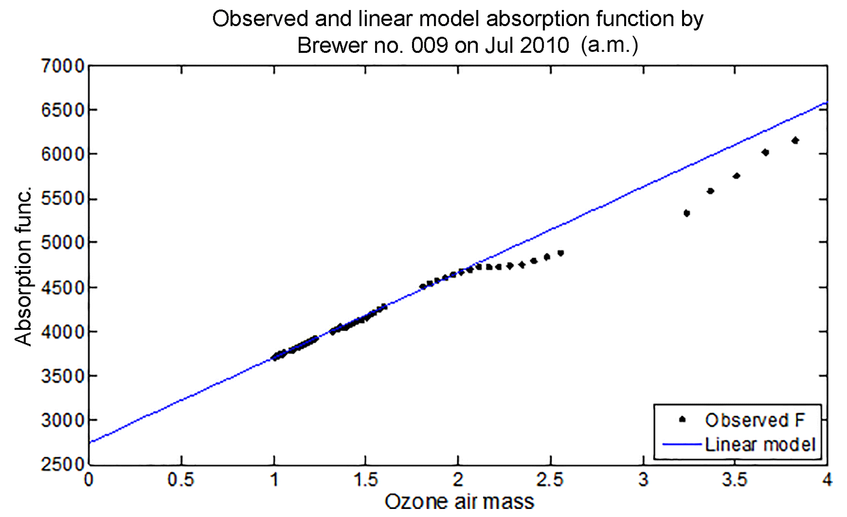
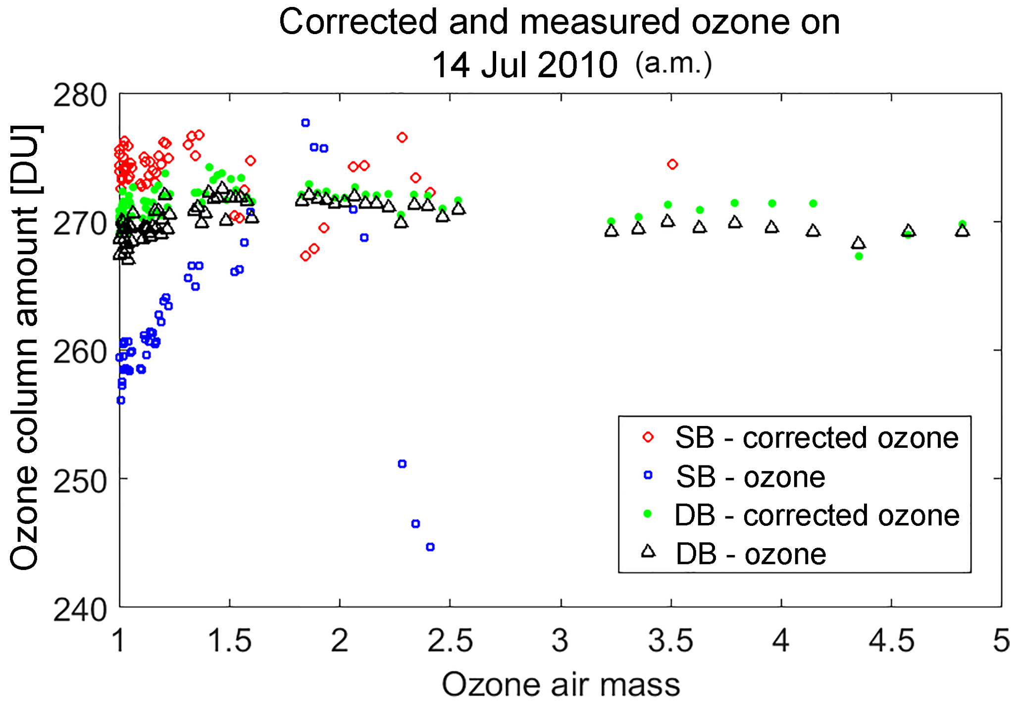
It is now known that single-monochromator Brewer spectrophotometer ozone and sulfur dioxide measurements suffer from non-linearity at large ozone slant column amounts due to the presence of instrumental stray light caused by scattering within the optics of the instrument. Because of the large gradient in the ozone absorption spectrum in the near-ultraviolet, the atmospheric spectra measured by the instrument possess a very large gradient in intensity in the 300 to 325 nm wavelength region. This results in a significant sensitivity to stray light when there is more than 1000 Dobson units (DU) of ozone in the light path. As the light path (air mass) through ozone increases, the stray-light effect on the measurements also increases. The measurements can be of the order of 10 %, low for an ozone column of 600 DU and an air mass factor of 3 (1800 DU slant column amount), which is an example of conditions that produce large slant column amounts.
Primary calibrations for the Brewer instrument are carried out at Mauna Loa Observatory in Hawaii and Izana Observatory in Tenerife. They are done using the Langley plot method to extrapolate a set of measurements made under a constant ozone vertical column to an extraterrestrial calibration constant. Since the effects of a small non-linearity at moderate ozone paths may still be important, a better calibration procedure should account for the non-linearity of the instrument response. Studies involving the scanning of a laser source have been used to characterize the stray-light response of the Brewer (Fioletov et al., 2000), but until recently these data have not been used to elucidate the relationship between the stray-light response and the ozone measurement non-linearity.
In a study done by Karppinen et al. (2015), a method for correcting stray light has been presented that uses an additive correction, which is determined via instrument slit characterization and a radiative transfer model simulation and is then applied to the single Brewer data (Karppinen et al., 2015). The European Brewer Network is also applying stray-light corrections, which includes an iterative process that results in correcting the single Brewer data to agree with double Brewer data (Rimmer et al., 2018; Redondas et al., 2018). The first model requires measurements of the slit function and the latter method relies on a calibrated instrument, such as a double Brewer, to characterize the instrument and to determine a correction for stray light.
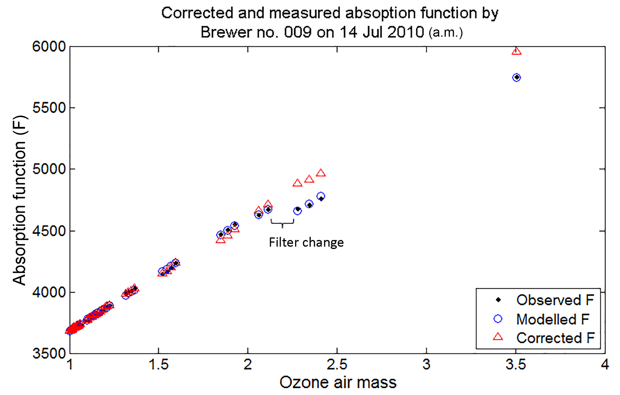
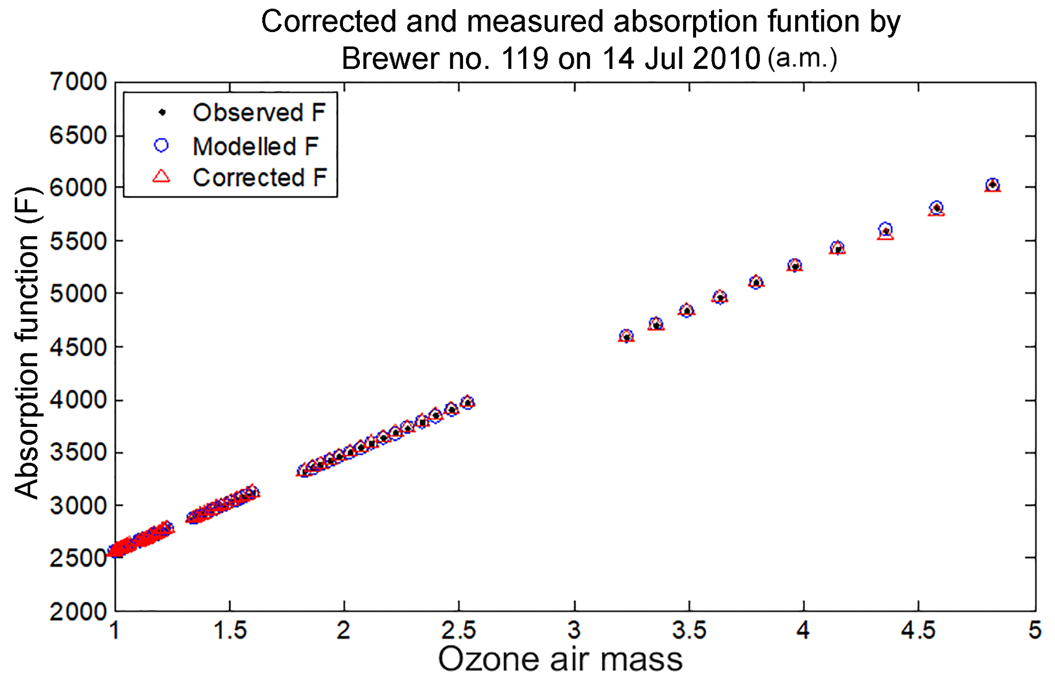
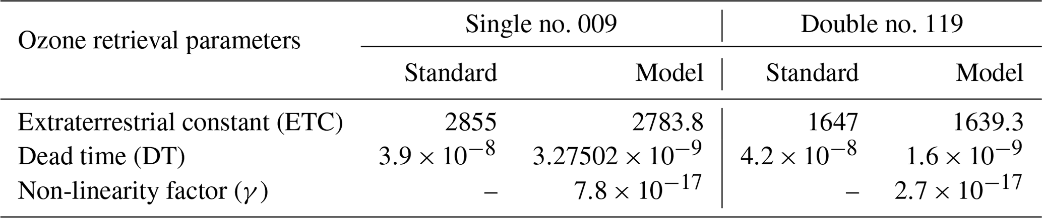
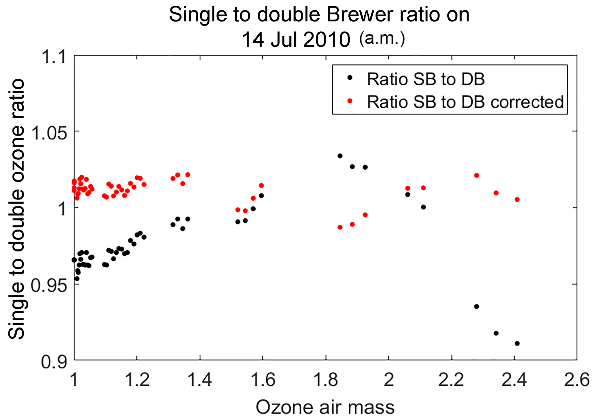
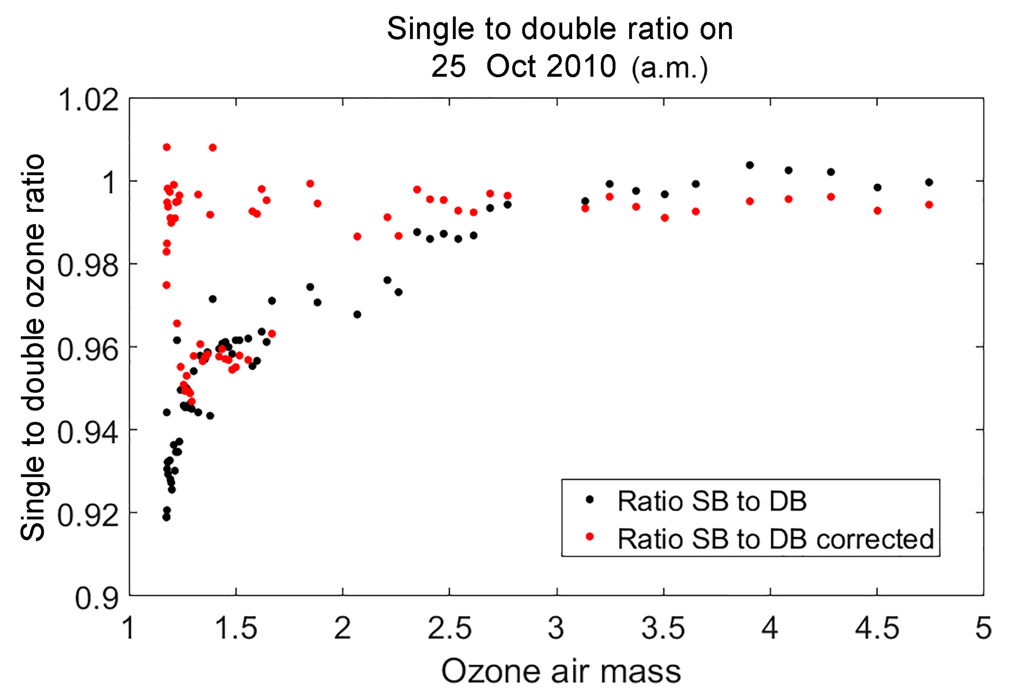
This paper presents a simple and practical method to correct for the effects of stray light, which includes a mathematical model of the instrument response and a non-linear retrieval approach that calculates the best values for the model parameters. The model can then be used in reverse to provide more accurate ozone values up to a defined maximum ozone slant path. The parameterization used was validated using an instrument physical model simulation. This model can be applied independently to any Brewer instrument and correct for the effects of stray light.