the Creative Commons Attribution 4.0 License.
the Creative Commons Attribution 4.0 License.
 | 14 May 2019
Is a scaling factor required to obtain closure between measured and modelled atmospheric O4 absorptions? An assessment of uncertainties of measurements and radiative transfer simulations for 2 selected days during the MAD-CAT campaign
Thomas Wagner
Steffen Beirle
Nuria Benavent
Tim Bösch
Ka Lok Chan
Sebastian Donner
Steffen Dörner
Caroline Fayt
Udo Frieß
David García-Nieto
Clio Gielen
David González-Bartolome
Laura Gomez
François Hendrick
Bas Henzing
Jun Li Jin
Johannes Lampel
Jianzhong Ma
Kornelia Mies
Mónica Navarro
Enno Peters
Gaia Pinardi
Olga Puentedura
Janis Puķīte
Julia Remmers
Andreas Richter
Alfonso Saiz-Lopez
Reza Shaiganfar
Holger Sihler
Michel Van Roozendael
Yang Wang
Margarita Yela
In this study the consistency between MAX-DOAS measurements and radiative transfer simulations of the atmospheric O4 absorption is investigated on 2 mainly cloud-free days during the MAD-CAT campaign in Mainz, Germany, in summer 2013. In recent years several studies indicated that measurements and radiative transfer simulations of the atmospheric O4 absorption can only be brought into agreement if a so-called scaling factor (<1) is applied to the measured O4 absorption. However, many studies, including those based on direct sunlight measurements, came to the opposite conclusion, that there is no need for a scaling factor. Up to now, there is no broad consensus for an explanation of the observed discrepancies between measurements and simulations. Previous studies inferred the need for a scaling factor from the comparison of the aerosol optical depths derived from MAX-DOAS O4 measurements with that derived from coincident sun photometer measurements. In this study a different approach is chosen: the measured O4 absorption at 360 nm is directly compared to the O4 absorption obtained from radiative transfer simulations. The atmospheric conditions used as input for the radiative transfer simulations were taken from independent data sets, in particular from sun photometer and ceilometer measurements at the measurement site. This study has three main goals: first all relevant error sources of the spectral analysis, the radiative transfer simulations and the extraction of the input parameters used for the radiative transfer simulations are quantified. One important result obtained from the analysis of synthetic spectra is that the O4 absorptions derived from the spectral analysis agree within 1 % with the corresponding radiative transfer simulations at 360 nm. Based on the results from sensitivity studies, recommendations for optimised settings for the spectral analysis and radiative transfer simulations are given. Second, the measured and simulated results are compared for 2 selected cloud-free days with similar aerosol optical depths but very different aerosol properties. On 18 June, measurements and simulations agree within their (rather large) uncertainties (the ratio of simulated and measured O4 absorptions is found to be 1.01±0.16). In contrast, on 8 July measurements and simulations significantly disagree: for the middle period of that day the ratio of simulated and measured O4 absorptions is found to be 0.82±0.10, which differs significantly from unity. Thus, for that day a scaling factor is needed to bring measurements and simulations into agreement. Third, recommendations for further intercomparison exercises are derived. One important recommendation for future studies is that aerosol profile data should be measured at the same wavelengths as the MAX-DOAS measurements. Also, the altitude range without profile information close to the ground should be minimised and detailed information on the aerosol optical and/or microphysical properties should be collected and used.
The results for both days are inconsistent, and no explanation for a O4 scaling factor could be derived in this study. Thus, similar but more extended future studies should be performed, including more measurement days and more instruments. Also, additional wavelengths should be included.


Observations of the atmospheric absorption of the oxygen collision complex (O2)2 (in the following referred to as O4; see Greenblatt et al., 1990) are often used to derive information about atmospheric light paths from remote-sensing measurements of scattered sunlight (for example made from ground, satellite, balloon or airplane). Since atmospheric radiative transport is strongly influenced by scattering on aerosol and cloud particles, information on the presence and properties of clouds and aerosols can be derived from O4 absorption measurements.
Early studies based on O4 measurements focussed on the effect of clouds (e.g. Erle et al., 1995; Wagner et al., 1998, 2014; Winterrath et al., 1999; Acarreta et al., 2004; Sneep et al., 2008; Heue et al., 2014; Gielen et al., 2014), which is usually stronger than that of aerosols. Later aerosol properties were also derived from O4 measurements, in particular from (multi-axis) MAX-DOAS measurements (e.g. Hönninger et al., 2004; Wagner et al., 2004, 2010; Wittrock et al., 2004; Frieß et al., 2006, 2016; Prados-Roman et al., 2011; Irie et al., 2008; Clémer et al., 2010, and references therein). For the retrieval of aerosol profiles forward model simulations for various assumed aerosol profiles are usually compared to measured O4 slant column densities (SCDs, the integrated O4 concentration along the atmospheric light path). The aerosol profile associated with the best fit between the forward model and measurement results is considered to be the most probable atmospheric aerosol profile (for more details, see e.g. Frieß et al., 2006). Note that in some cases no unique solution might exist if different atmospheric aerosol profiles lead to the same O4 absorptions. MAX-DOAS aerosol retrievals are typically restricted to altitudes below about 4 km; see Frieß et al. (2006).
About 10 years ago, Wagner et al. (2009) suggested applying a scaling factor (SF<1) to the O4 SCDs derived from MAX-DOAS measurements at 360 nm in Milan in order to achieve agreement with forward model simulations. They found that on a day with low aerosol load the measured O4 SCDs were larger than the model results, even if no aerosols were included in the model simulations. If, however, the measured O4 SCDs were scaled by an SF of 0.81, good agreement with the forward model simulations (and nearby AERONET measurements) was achieved. Similar findings were then reported by Clémer et al. (2010), who suggested an SF of 0.8 for MAX-DOAS measurements in Beijing. Interestingly, they applied this SF to four different O4 absorption bands (360, 477, 577 and 630 nm).
While with the application of an SF the consistency between forward model and measurements was substantially improved, neither study could provide an explanation for the physical mechanism behind such an SF. In the following years several research groups applied an SF in their MAX-DOAS aerosol profile retrievals. However, a similarly large fraction of studies (including direct sun measurements and aircraft measurements; see Spinei et al., 2015) did not find it necessary to apply an SF to bring measurements and forward model simulations into agreement. An overview of the application of an SF to various MAX-DOAS publications after 2010 is provided in Table 1. Up to now, there is no community consensus on whether or not an SF is needed for measured O4 dSCDs. This is a rather unfortunate situation, because this ambiguity directly affects the aerosol results derived from MAX-DOAS measurements and thus the general confidence in the method.
Table 1Overview of studies which did not apply a scaling factor (upper part) or did apply a scaling factor (lower part) to the measured O4 dSCDs. Besides the initial studies proposing a scaling factor (Wagner et al., 2009; Clémer et al., 2010), only studies after 2010 are listed.
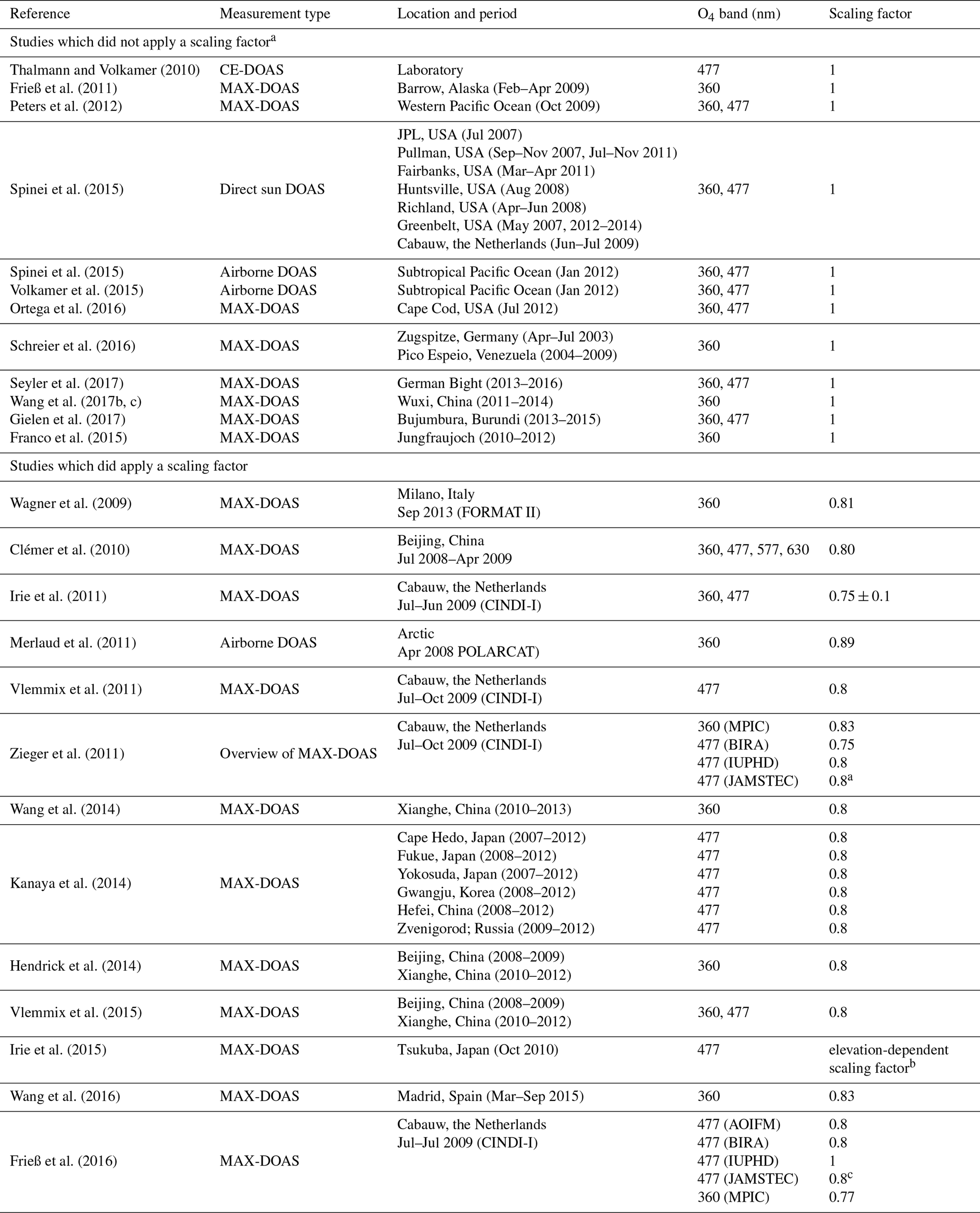
a The authors of part of these studies were probably not aware that a scaling
factor was applied by other groups.
b .
c SF is varied during profile inversion.
So far, most of the studies deduced the need for an SF in a rather indirect way: aerosol extinction profiles derived from MAX-DOAS measurements using different SF are usually compared to independent data sets (mostly aerosol optical depth, AOD, from sun photometer observations) and the SF leading to the best agreement is selected. In many cases SF between 0.75 and 0.9 were derived.
In this study, we follow a different approach: similarly to Ortega et al. (2016) we directly compare the measured O4 SCDs with the corresponding SCDs derived with a forward model (consisting of a radiative transfer model and assumptions of the state of the atmosphere). For this comparison, atmospheric conditions which are well characterised by independent measurements are chosen. In particular, such a procedure allows the influence of the uncertainties of the individual processing steps to be quantified.
One peculiarity of this comparison is that the measured O4 SCDs are first converted into their corresponding air mass factors (AMFs), which are defined as the ratio of the SCD and the vertical column density (VCD, the vertically integrated concentration) (Solomon et al., 1987).
The “measured” O4 AMF is then compared to the corresponding AMF derived from radiative transfer simulations for the atmospheric conditions during the measurements:
The conversion of the measured O4 SCDs into AMFs is carried out to ensure a simple and direct comparison between measurements and forward model simulations. Here it should be noted that in addition to the AMFs so-called differential AMFs (dAMFs) will be compared in this study. The dAMFs represent the difference between AMFs for measurements at non-zenith elevation angles α and at 90∘ for the same elevation sequence:
Note that in this paper the following notations are used:
-
AMF is the air mass factor.
-
dAMF is the differential air mass factor.
-
(d)AMF is the air mass factor and/or differential air mass factor (similar notations are used for the (d)SCDs).
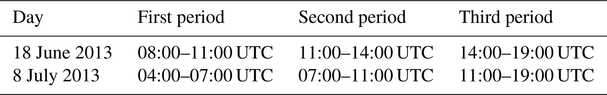
For the comparison between measured and simulated O4 (d)AMFs, 2 mostly cloud-free days (18 June and 8 July 2013) during the Multi Axis DOAS Comparison campaign for Aerosols and Trace gases (MAD-CAT) campaign are chosen (http://joseba.mpch-mainz.mpg.de/mad_cat.htm, last access: 29 April 2019). As discussed in more detail in Sect. 4.2.2, based on the ceilometer and sun photometer measurements, three periods on each of the 2 selected days are selected, during which the variation of the aerosol profiles was relatively small (see Table 2). In addition to the aerosol profiles, other atmospheric properties are averaged during these periods before they are used as input for the radiative transfer simulations.
Table 2Periods on both selected days, which are used for the comparisons.
The comparison is carried out for the O4 absorption band at 360 nm, which is the strongest O4 absorption band in the UV. In principle other O4 absorption bands (e.g. in the visible spectral range) could also be chosen, but these bands are not covered by the wavelength range of the MPIC instrument. Thus, they are not part of this study.
The comparison between measurements and simulations is performed in three different steps: first, for selected periods in the middle of each day, the ratios between measured and simulated O4 (d)AMFs are calculated for “standard settings” of the spectral retrieval and radiative transfer simulations (for details see below). In a second step, the uncertainties of the measurements and simulations are investigated. In the final step, it is investigated whether the ratio of measured and simulated O4 (d)AMFs agree with unity when taking into account these uncertainties.
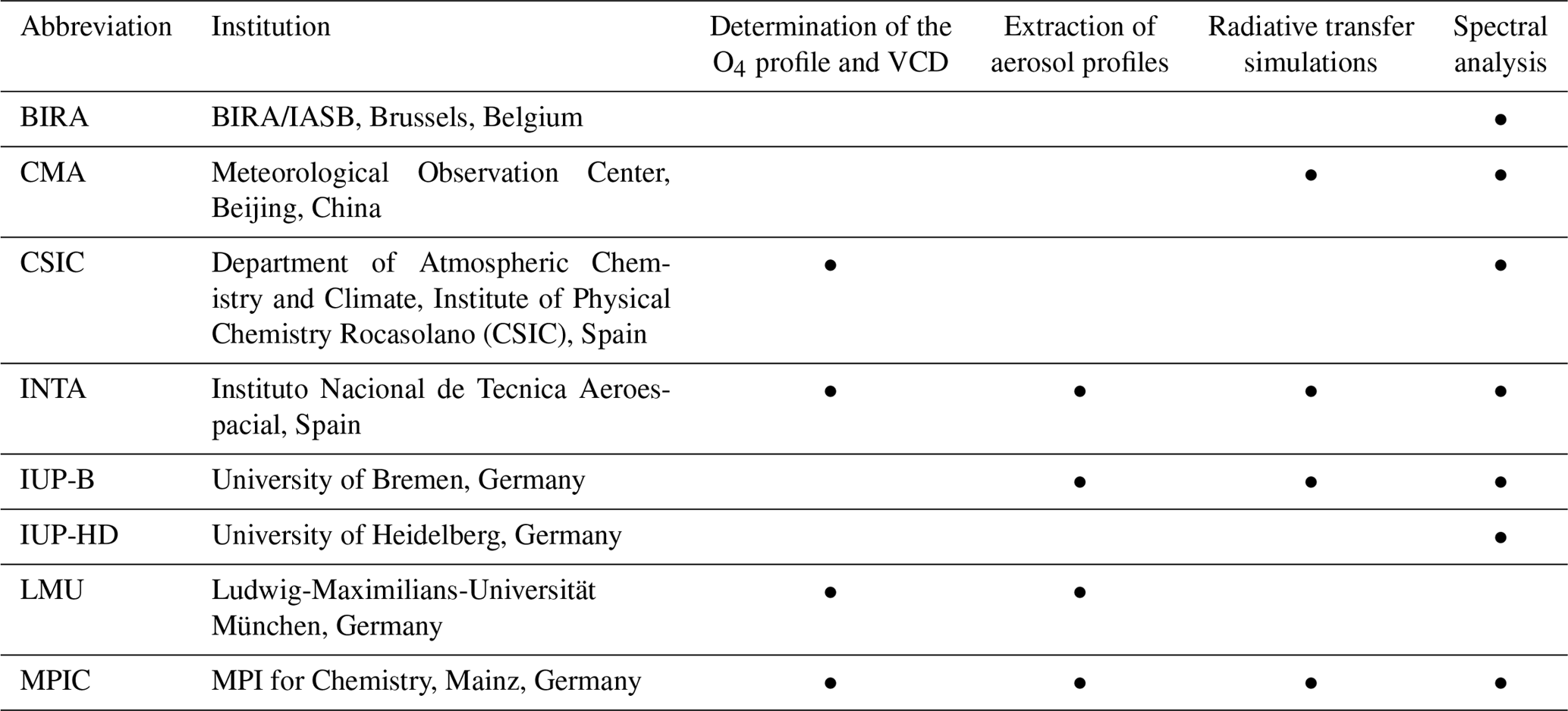
Table 3Participation of the different groups in the different analysis steps.
Deviations between the forward model and measurements can have different causes. In the following an overview of these error sources and the way they are investigated in this study are given:
-
Calculation of O4 profiles and O4 VCDs (Eq. 1).
Profiles and VCDs of O4 are derived from pressure and temperature profiles. The uncertainties of the pressure and temperature profiles are quantified by sensitivity studies and by the comparison of the extraction results derived from different groups or persons (see Table 3).
-
Calculation of O4 (d)AMFs from radiative transfer simulations.
Besides differences between the different radiative transfer codes, the dominating sources of uncertainty are those related to the input parameters. They are investigated by sensitivity studies and by the comparison of extracted input data by different groups or persons. Also, the effects of operating different radiative transfer models by different groups are investigated.
-
Analysis of the O4 (d)AMFs from MAX-DOAS measurements.
Uncertainties in the spectral analysis results are caused by errors and imperfections in the measurements and instruments, the dependence of the analysis results on the specific fit settings and the uncertainties of the O4 cross sections including their temperature dependence. They are investigated by systematic variation of the DOAS fit settings (for measured and synthetic spectra) and by comparison of analysis results obtained from different groups and/or instruments.
The paper is organised as follows: in Sect. 2, information on the selected days during the MAD-CAT campaign, on the MAX-DOAS measurements and on the data sets from independent measurements is provided. Section 3 presents the initial comparison results for the selected days using standard settings. In Sect. 4 the uncertainties associated with each of the various processing steps of the spectral analysis and the forward model simulations are quantified by being compared to the results for the standard settings. Section 5 presents a summary and conclusions.
The Multi Axis DOAS Comparison campaign for Aerosols and Trace gases (MAD-CAT) (http://joseba.mpch-mainz.mpg.de/mad_cat.htm) took place in June and July 2013 on the roof of the Max Planck Institute for Chemistry in Mainz, Germany. The main aim of the campaign was to compare MAX-DOAS retrieval results of several atmospheric trace gases like NO2, HCHO, HONO and CHOCHO as well as aerosols. The measurement location was at 150 m above sea level at the western edge of the city of Mainz.
2.1 MAX-DOAS instruments
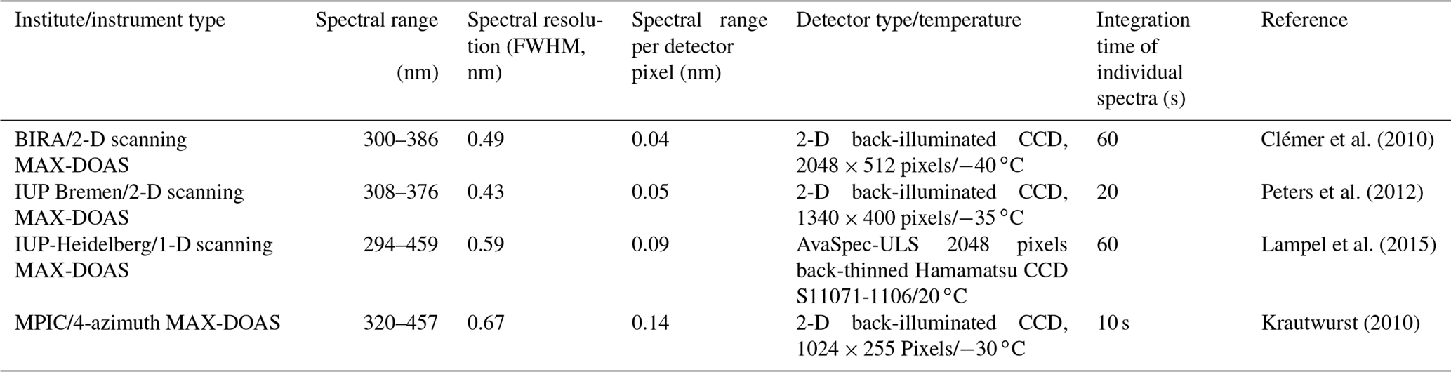
During the MAD-CAT campaign, 11 MAX-DOAS instruments were operated by different groups; an overview can be found at the website http://joseba.mpch-mainz.mpg.de/equipment.htm (last access: 29 April 2019). The main viewing direction of the MAX-DOAS instruments was towards north-west (51∘ with respect to north). Measurements at this viewing direction were the main focus of this study, but a few comparisons using the standard settings (see Sect. 3) were also carried out for three other azimuth angles (141, 231, 321∘; see Fig. A2I in Appendix A1). Each elevation sequence contains the following elevation angles: 1, 2, 3, 4, 5, 6, 8, 10, 15, 30 and 90∘. In this study, in addition to the MPIC instrument, spectra from three other MAX-DOAS instruments were also analysed. The instrument details are given in Table 4. The spectra of the MPIC instrument are available at the website http://joseba.mpch-mainz.mpg.de/e_doc_zip.htm (last access: 29 April 2019).
Table 4Overview of properties of MAX-DOAS instruments participating in this study.
2.2 Additional data sets
In order to constrain the radiative transfer simulations, independent measurements and data sets were used. In particular, information on atmospheric pressure, temperature and relative humidity, as well as aerosol properties, is used. In addition to local in situ measurements from air quality monitoring stations and remote-sensing measurements by a ceilometer and a sun photometer, ECMWF reanalysis data were used. An overview of these data sets is given in Table 5. The data sets used in this study are available at the websites http://joseba.mpch-mainz.mpg.de/a_doc_zip.htm (last access: 29 April 2019) and http://joseba.mpch-mainz.mpg.de/c_doc_zip.htm (last access: 29 April 2019).
Table 5Independent data sets used to constrain the atmospheric properties on both selected days.
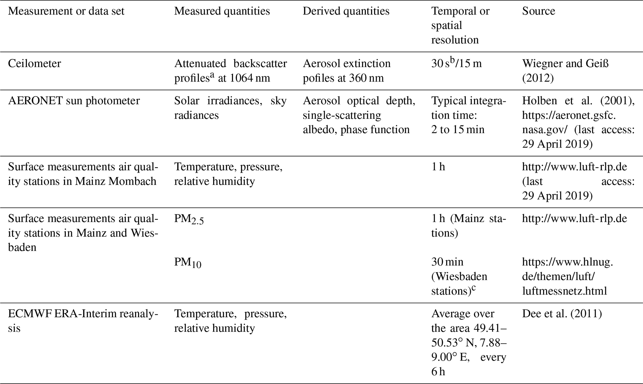
a There is no useful signal below 180 m due to limited overlap.
b Here 15 min averages are used.
c Stations in Mainz are Parcusstrasse, Zitadelle and Mombach. Stations in
Wiesbaden are Schierstein, Ringkirche and Süd.
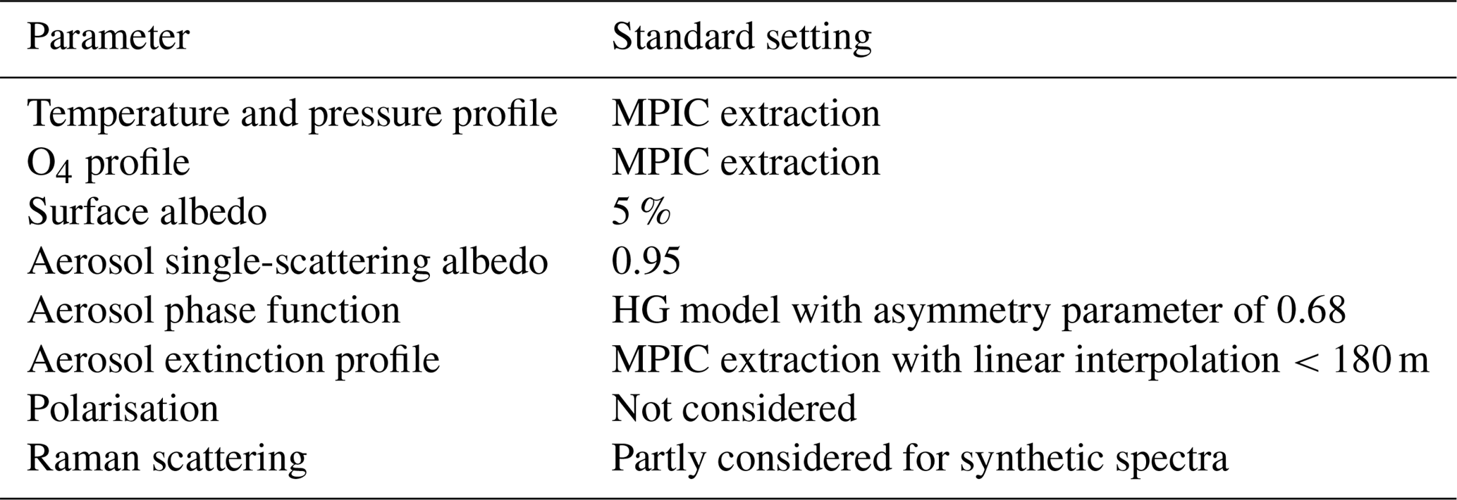
2.3 RTM simulations
Several radiative transfer models are used to calculate O4 (d)AMFs for the selected days. As input, vertical profiles of temperature, pressure, relative humidity and aerosol extinction extracted from the independent data sets (see Sects. 2.2 and 4) were used. The vertical resolution is high in the lowest layers and decreases with increasing altitude (see Table A1 in Appendix A1). The upper boundary of the vertical grid is set to 1000 km. The lower boundary of the model grid represents the surface elevation of the instrument (150 m above sea level). For the standard run, a surface albedo of 5 % is assumed and the aerosol optical properties are described by a Henyey–Greenstein phase function with an asymmetry parameter of 0.68 and a single-scattering albedo of 0.95. Both values represent typical urban aerosols (see e.g. Dubovik et al., 2002). Ozone absorption was not considered, because it is very small at 360 nm. The MAD-CAT campaign took place around the summer solstice. Thus, the same dependence of the solar zenith angle (SZA) and relative azimuth angle (RAZI) on time is used for both days (see Table A2 in the Appendix A1). The input data used for the radiative transfer simulations are available at the website http://joseba.mpch-mainz.mpg.de/d_doc_zip.htm (last access: 29 April 2019). In the following subsections the different radiative transfer models used in this study are described.
2.3.1 McArtim
The full spherical Monte Carlo radiative transfer model, McArtim (Deutschmann et al., 2011), explicitly simulates individual photon trajectories including the photon interactions with molecules, aerosol particles and the surface. In this study, two versions of McArtim are used: version 1 and version 3. Version 1 is a 1-D scalar model. Version 3 can also be run in 3-D and vector modes. In version 1 rotational Raman scattering (RRS) is partly taken into account: the RRS cross section and phase function are explicitly considered for the determination of the photon paths, but the wavelength redistribution during the RRS events is not considered. In version 3 RRS can be fully taken into account. If operated in the same mode (1-D scalar), both models show excellent agreement.
2.3.2 LIDORT
In this study the LIDORT version 3.3 was used. The Linearized Discrete Ordinate Radiative Transfer (LIDORT) forward model (Spurr et al., 2001, 2008) is based on the discrete ordinate method to solve the radiative transfer equation (e.g. Chandrasekhar, 1960, 1989; Stamnes et al., 1988). This model considers a pseudo-spherical multilayered atmosphere including several anisotropic scatters. The formulation implemented corrects for the atmosphere curvature in the solar and single-scattered beams; however the multiple-scattering term is treated in the plane-parallel approximation. The properties of each of the atmospheric layers are considered homogenous in the corresponding layer. Using finite differences for the altitude derivatives, this linearised code converts the problem into a linear algebraic system. Through first-order perturbation theory, it is able to provide radiance field and radiance derivatives with respect to atmospheric and surface variables (Jacobians) in a single call. LIDORT was used in several studies to derive vertical profiles of aerosols and trace gases from MAX-DOAS (e.g. Clémer et al., 2010; Hendrick et al., 2014; Franco et al., 2015).
2.3.3 SCIATRAN
The RTM SCIATRAN (Rozanov et al., 2014) was used in its full-spherical mode including multiple scattering but without polarisation. In the operation mode used here, SCIATRAN solves the transfer equations using the discrete ordinate method. In this study, SCIATRAN was used by two groups: the IUP Bremen group used v3.8.3 for the O4 dAMFs simulations (without Raman scattering). The MPIC group used v3.6.11 for the calculation of synthetic spectra (see Sect. 2.4) and for the O4 dAMFs simulations (including Raman scattering).
2.4 Synthetic spectra
In addition to AMFs and dAMFs, synthetic spectra were simulated. They are analysed in the same way as the measured spectra, which allows the investigation of two important aspects:
-
The derived O4 dAMFs from the synthetic spectra can be compared to the O4 dAMFs obtained directly from the radiative simulations at one wavelength (here, 360 nm) using the same settings. In this way the consistency of the spectral analysis results and the radiative transfer simulations is tested.
-
Sensitivity tests can be performed by varying several fit parameters, e.g. the spectral range or the DOAS polynomial, and their effect on the derived O4 dAMFs can be assessed.
Synthetic spectra are simulated using SCIATRAN while taking into account rotational Raman scattering. The basic simulation settings are the same as for the RTM simulations of the O4 (d)AMFs described above. In order to minimise the computational effort, for the profiles of temperature, pressure, relative humidity and aerosol extinction the input data for only two periods (18 June on 11:00–14:00 UTC, 8 July on 07:00–11:00; see Table 2) are used for the whole day. Thus, “perfect” agreement with the measurements can only be expected for the two selected periods. Aerosol optical properties (phase function and single-scattering albedo) are taken from AERONET measurements of the 2 selected days. Although the wavelength dependencies of both quantities (and also for the aerosol extinction) are considered, it should be noted that the associated uncertainties are probably rather large, since the optical properties in the UV had to be extrapolated from measurements in the visible spectral range.
Spectra were simulated at a spectral resolution of 0.01 nm and convolved with a Gaussian slit function of 0.6 nm full width at half maximum (FWHM), which is similar to those of the measurements. For the generation of the spectra a high-resolution solar spectrum (Chance and Kurucz, 2010) and the trace gas absorptions of O3, NO2, HCHO and O4 are considered (see Table A3 in Appendix A1). The assumed tropospheric profiles of NO2 and HCHO are similar to those retrieved from the MAX-DOAS observations during the selected periods. Time series of the tropospheric VCDs of NO2 and HCHO for the 2 selected days are shown in Fig. A1 in Appendix A1.
Two sets of synthetic spectra were simulated, one taking into account the temperature dependence of the O4 cross section and the other not. For the case that not consider the temperature dependence, the O4 cross section for 293 K is used. In addition to spectra without noise, spectra with noise (sigma of the noise is assumed as times the intensity) were simulated. The synthetic spectra are available at the website http://joseba.mpch-mainz.mpg.de/f_doc_zip.htm (last access: 29 April 2019).
3.1 Selection of days
For the comparison of measured and simulated O4 dAMFs, 2 mostly cloud-free days during the MAD-CAT campaign (18 June and 8 July 2013) were selected. On both days the AOD measured by the AERONET sun photometer at 360 nm was between 0.25 and 0.4 (see Fig. 1). In spite of the similar AODs, very different aerosol properties at the surface were found on the 2 selected days: on 18 June much higher concentrations of large aerosol particles (PM2.5 and PM10) are found. These differences are also represented by the large differences in the Ångström exponent for long wavelengths (440–870 nm) on both days. Also, the aerosol height profiles are different: on 8 July rather homogenous profiles with a layer height of about 2 km occur. On 18 June the aerosol profiles reach higher altitudes, but the highest extinction is found close to the surface. Also, the temporal variability of the aerosol properties, especially the near-surface concentrations, is much larger on 18 June.
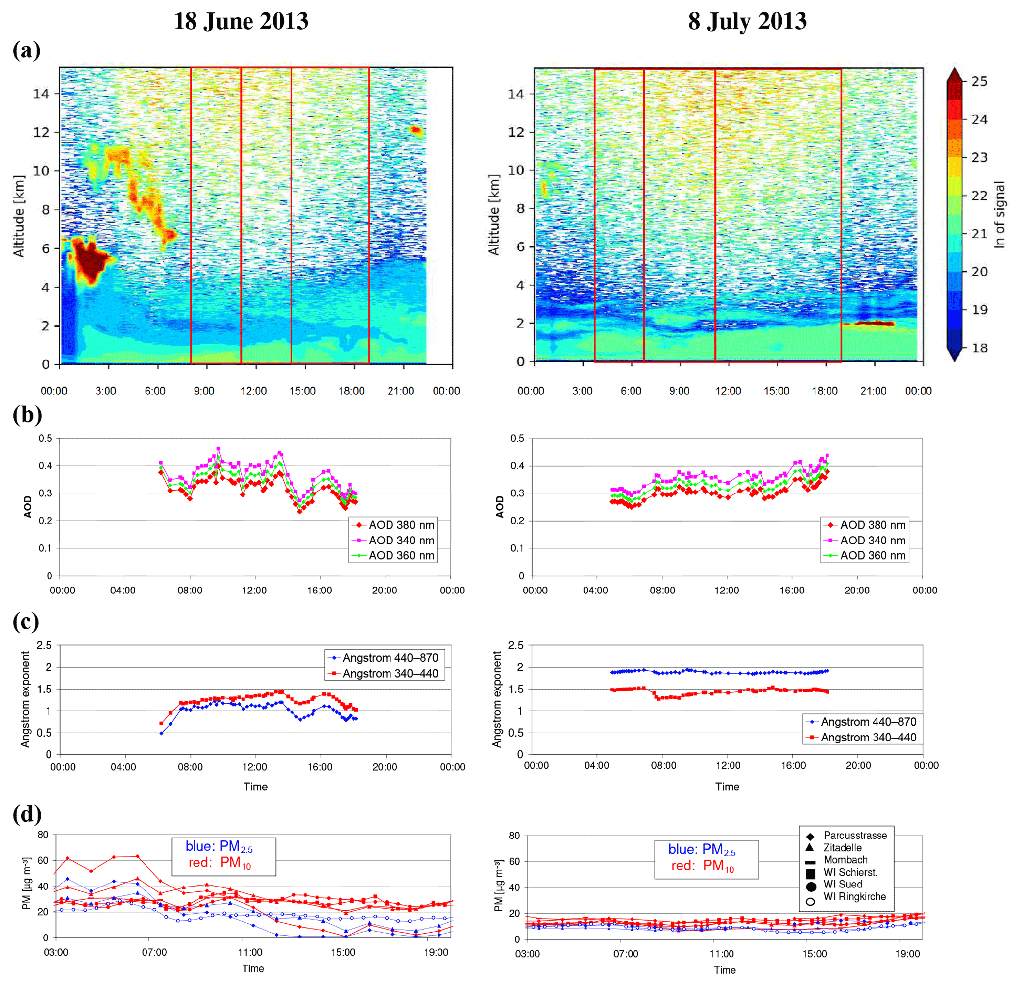
Figure 1Various aerosol properties on the 2 selected days (left: 18 June 2013; right: 8 July 2013). (a) Aerosol backscatter profiles from ceilometer measurements. (b) AOD at 340, 360 and 380 nm (360 values are interpolated from 340 and 380 nm) from AERONET sun photometer measurements. (c) Ångström exponents for two wavelength pairs (340–440 and 440–870 nm) from AERONET sun photometer measurements. (d) Surface in situ measurements of PM2.5 and PM10 measured at different air quality monitoring stations in Mainz and the nearby city of Wiesbaden.
3.2 Different levels of comparisons
The comparison between the forward model and MAX-DOAS measurements is performed at different depths for different subsets of the measurements:
-
A quantitative comparison of O4 AMFs and O4 dAMFs is performed for 3∘ elevation angle at the standard viewing direction (51∘ with respect to north) for the middle period of each selected day. During these periods the uncertainties of the measurement and the radiative transfer simulations are smallest because around noon the measured intensities are high and the variation of the SZA is small. During the selected periods, the variation of the ceilometer profiles is also relatively small. These comparisons thus constitute the core of the comparison exercise and all sensitivity studies are performed for these two periods. The elevation angle of 3∘ is selected because for such a low-elevation angle the atmospheric light paths and thus the O4 absorption is rather large. Moreover, as can be seen in Fig. 2, the O4 (d)AMFs for 3∘ are very similar to those for 1 and 6∘, especially on 8 July 2013. Sensitivity studies showed that a wrong elevation angle calibration (±0.5∘) led to only small changes (<1 %) in the O4 (d)AMFs. Changes in the field of view between 0.2 and 1.1∘ led to even smaller differences. These findings indicate that possible uncertainties of the calibration of the elevation angles of the instruments can be neglected. Here it is interesting to note that on 18 June even slightly lower O4 (d)AMFs are found for the low-elevation angles. This is in agreement with the finding of high aerosol extinction in a shallow layer above the surface (see Fig. 1). The azimuth angle of 51∘ was chosen, because it was the standard viewing direction during the MAD-CAT campaign and measurements for this direction are available from different instruments.
-
The quantitative comparison for 3∘ elevation and an azimuth of 51∘ is also extended to the periods prior to and after the middle periods of the selected days. However, to minimise the computational efforts, some sensitivity studies are not carried out for the first and last periods.
-
The comparison is extended to more elevation angles (1, 3, 6, 10, 15, 30, 90∘) and azimuth angles (51, 141, 231, 321∘). For this comparison only the standard settings for the DOAS analysis and the radiative transfer simulations are applied (see Tables 6 and 7). The comparison results for the MPIC MAX-DOAS measurements are shown in Appendix A2. The purpose of this comparison is to check whether for other viewing angles similar results are found as for 3∘ elevation at 51∘ azimuth direction.
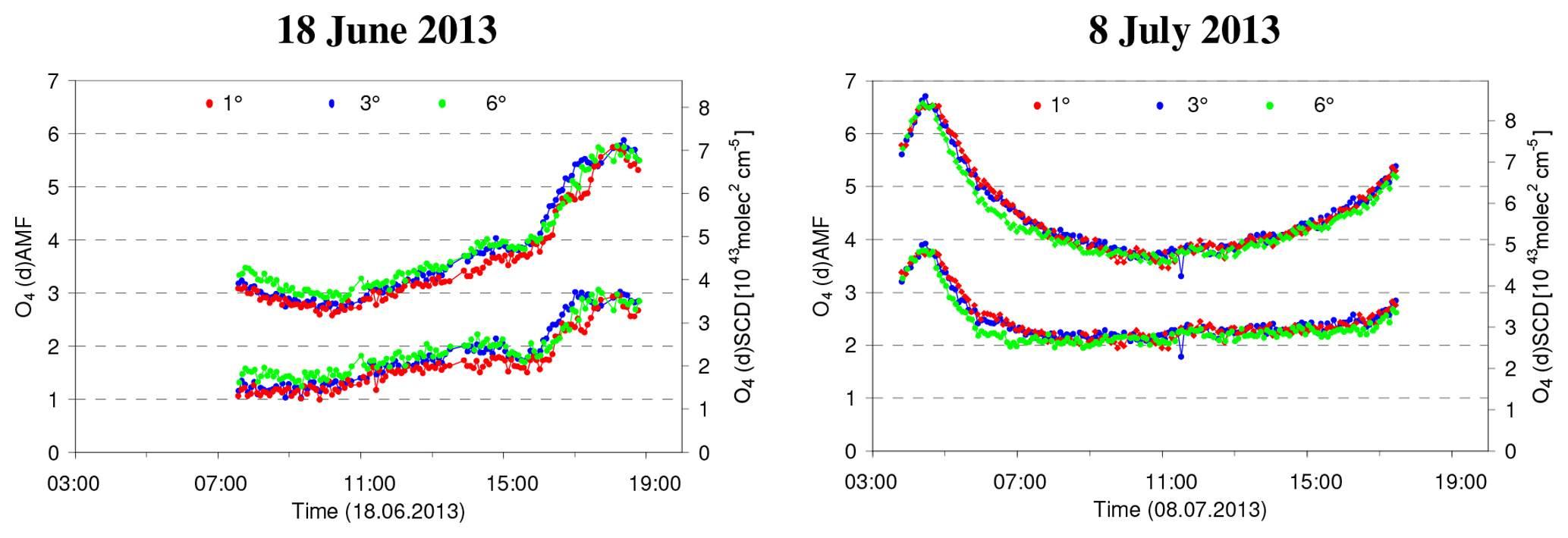
Figure 2O4 AMFs (upper lines) and dAMFs (lower lines) for 1, 3 and 6∘ elevation angles derived from the MPIC MAX-DOAS measurements on the 2 selected days. Interestingly, on 18 June the lowest values are in general found for the lowest elevation angles, which is an indication for the high aerosol load close to the surface. The y axis on the right shows the corresponding O4 (d)SCDs for O4 VCDs of 1.23×1043 molecules2 cm−5 and 1.28×1043 molecules2 cm−5 for 18 June and 8 July, respectively (see Sect. 4.1.2).
Table 6Standard settings for the radiative transfer simulations.
3.3 Quantitative comparison for 3∘ elevation in standard azimuth direction
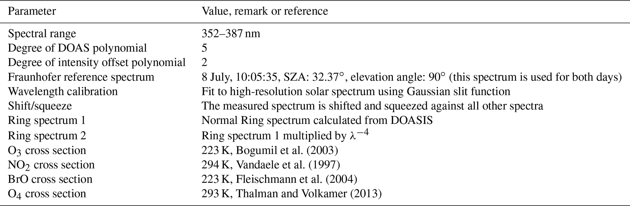
Figure 3 presents a comparison of the measured and simulated O4 (d)AMFs for 3∘ elevation and 51∘ azimuth on both days. For the spectral analysis and the radiative transfer simulations the respective standard settings (see Tables 6 and 7) were used. On 8 July the simulated O4 (d)AMFs systematically underestimate the measured O4 (d)AMFs by up to 40 %. Similar results are obtained for other elevation and azimuth angles (see Appendix A2), with the differences becoming smaller towards higher elevation angles. In contrast, no systematic underestimation is observed for most of 18 June. For some periods of that day the simulated O4 (d)AMFs are even larger than the measured O4 (d)AMFs. However, here it should be noted that the aerosol extinction profile of the standard settings (using linear extrapolation below 180 m where no ceilometer data are available) probably underestimates the aerosol extinction close to the surface. If instead a modified aerosol profile with strongly increased aerosol extinction below 180 m and the maximum AOD during that period is used (see Fig. A31 in Appendix A5), the corresponding (d)AMFs fall below the measured O4 (d)AMFs (green curves in Fig. A4 in Appendix A2). More details on the extraction of the aerosol extinction profiles are given in Sect. 4.2.2 and Appendix A5).
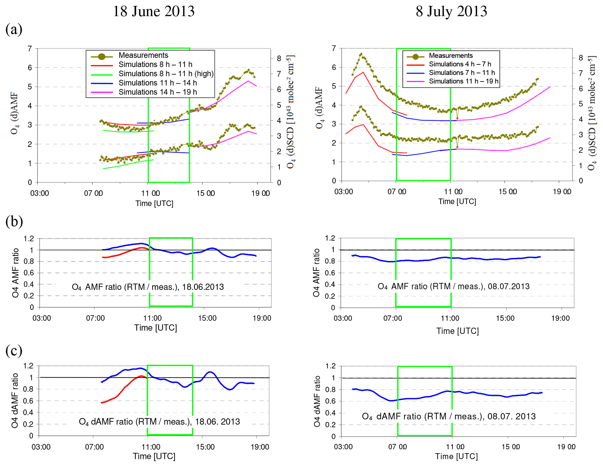
Figure 3(a) Comparison of O4 (d)AMFs from MAX-DOAS measurements and forward model simulations for the 2 selected days. The green rectangle indicates the middle period on each day, which are the focus of the quantitative comparison. The green line on 18 June represents forward model results for a modified aerosol profile (see text). The y axis on the right shows the corresponding O4 (d)SCDs for O4 VCDs of 1.23×1043 molecules2 cm−5 and 1.28 ⋅ 1043 molecules2 cm−5 for 18 June and 8 July, respectively (see Sect. 4.1.2). In (b) and (c) the ratios of the simulated and measured AMFs and dAMFs are shown, respectively. The red line on 18 June represents the ratios for the modified aerosol scenario.
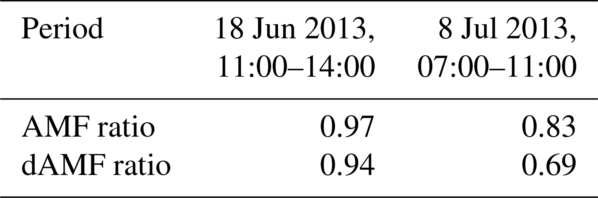
The average ratio of simulated to measured (d)AMFs (for the standard settings) during the middle period on each day are given in Table 8. For 18 June they are close to unity, but for 8 July they are much lower (0.83 for the AMF and 0.69 for the dAMF).
Table 8Average ratios (simulation results divided by measurements) of the O4 (d)AMFs for the middle periods of the selected days.
There are three major processing steps, for which the uncertainties are quantified in this section:
-
the determination of the O4 height profiles and corresponding O4 VCDs,
-
the simulation of O4 (d)AMFs by the forward model,
-
the analysis of O4 (d)AMFs from the MAX-DOAS measurements.
4.1 Determination of the vertical O4 profile and the O4 VCD
The O4 VCD is required for conversion of measured (d)SCDs into (d)AMFs (Eq. 1). O4 profiles are also needed for the calculation of O4 (d)AMFs. The accuracy of the calculated O4 height profile and the O4 VCD depends in particular on two aspects:
-
Is profile information on temperature, pressure and (relative) humidity available?
-
What is the accuracy of these data sets?
Additional uncertainties are related to the details of the calculation of the O4 concentration and O4 VCDs from these profiles. Both sources of uncertainties are investigated in the following subsections.
4.1.1 Extraction of vertical profiles of temperature and pressure
The procedure of extracting temperature and pressure profiles depends on the availability of measured profile data or surface measurements. If profile data are available (e.g. from sondes or models) they could be directly used. If only surface measurements are available, vertical profiles of temperature and pressure could be calculated by making assumptions on the lapse rate (here we assume a value of ). If no measurements or model data are available, profiles from the US standard atmosphere might be used (United States Committee on Extension to the Standard Atmosphere, 1976). In Appendix A3 the different procedures for the extraction of pressure and temperature profiles are described in detail for the 2 selected days of the MAD-CAT campaign. For these days the optimum choice was to combine the model data and the surface measurements. In that way, the diurnal variation in the boundary layer could be considered. In Fig. 4 temperature and pressure profiles extracted from the combination of in situ measurements and ECMWF data are shown. These profiles probably best match the true atmospheric profiles.
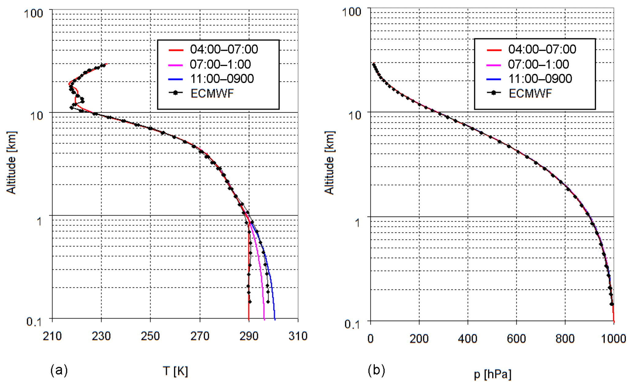
Figure 4Extracted temperature (a) and pressure (b) profiles for the three periods on 8 July 2013. Also shown are ECMWF profiles above Mainz for 06:00 and 18:00. To better account for the diurnal variation of the temperatures near the surface, below 1 km the temperature is linearly interpolated between the surface measurements and the ECMWF temperatures at 1 km (for details see text). Note that the altitude is given relative to the height of the measurement site (150 m).
A comparison of temperature profiles extracted by different methods for two selected periods on both days is shown in Fig. 5. For 8 July (right), a rather good agreement is found, but for 18 June (left) the agreement is worse (differences up to 20 K). Of course, the differences between the true and the US standard atmosphere profiles can become even larger, depending on location and season. So the use of a fixed temperature and pressure profile should always be the last choice. In contrast, the simple extrapolation from surface values can be very useful if no profile data are available, because the uncertainties of this method are usually smallest at low altitudes, where the bulk of O4 is located.
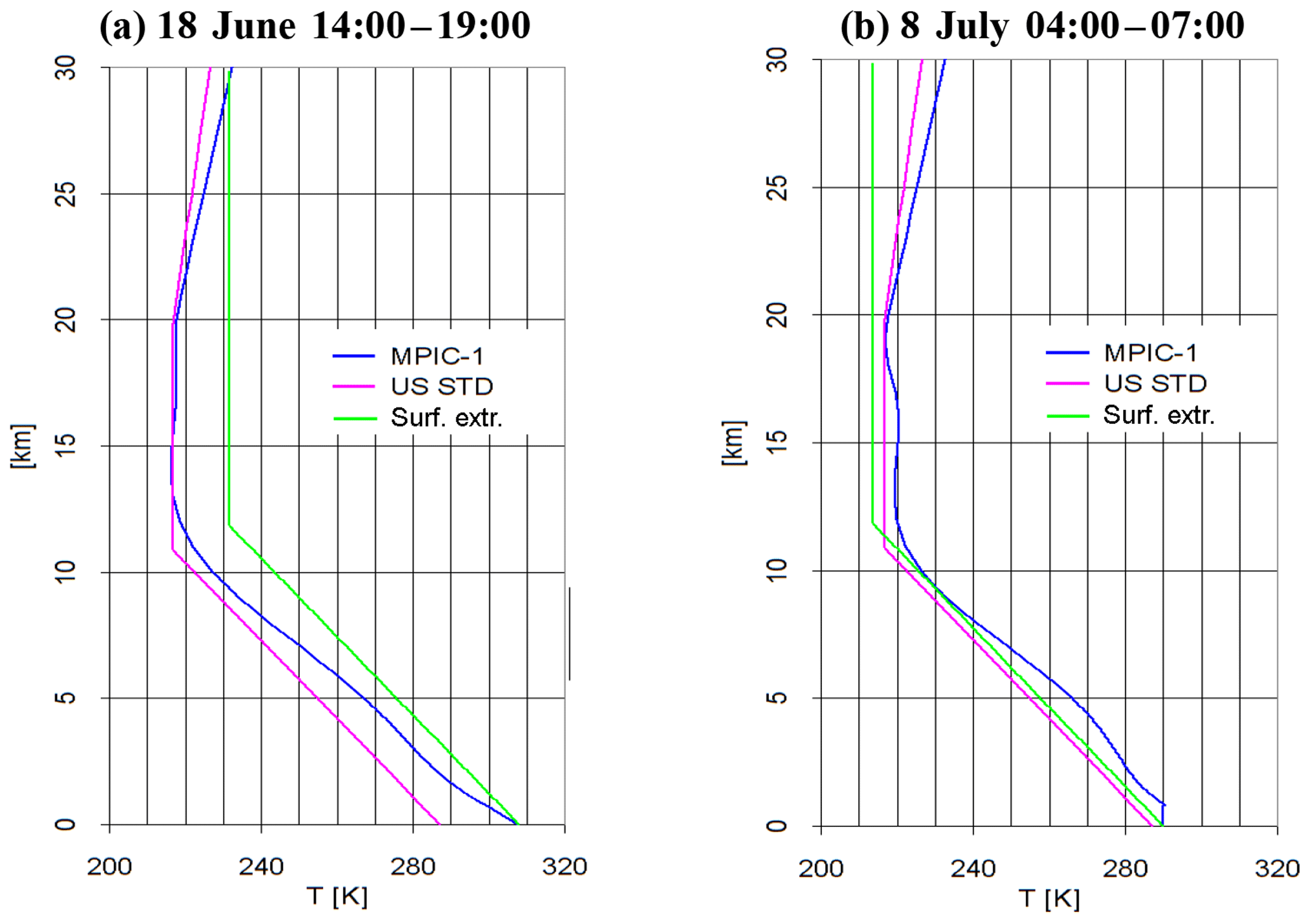
Figure 5Temperature profiles extracted in different ways for two periods, (a 18 June, 14:00–19:00 and b 8 July, 04:00–07:00). The blue profiles are extracted from in situ measurements and ECMWF profiles as described in the text. The green profiles are extracted from the surface temperatures and assume a constant lapse rate of up to 12 km and a constant temperature above. The pink curves represent the temperature profile from the US standard atmosphere.
4.1.2 Calculation of O4 concentration profiles and O4 VCDs
From the temperature and pressure profiles the oxygen (O2) concentration is calculated. Here, the effect of the atmospheric humidity profiles should also be taken into account (see Appendix A3), because it can have a considerable effect on the near-surface layers (at least for temperatures of about >20 ∘C). Finally, the square of the oxygen concentration is calculated and used as proxy for the O4 concentration consistently with assumptions made in the determination of the absorption cross sections (see Greenblatt et al., 1990). The uncertainties of the derived O4 concentration (and the corresponding O4 VCD) caused by the uncertainty of the input profiles is estimated by varying the input parameters (for details see Appendix A3).
For both selected days during the MAD-CAT campaign the total uncertainty is estimated to be about 1.5 % assuming that the uncertainties of the individual input parameters are independent.
Further uncertainties arise from the procedure of the vertical integration of the O4 concentration profiles. We tested the effect of using different vertical grids and altitude ranges. It is found that the vertical grid should not be coarser than 100 m (for which a deviation in the O4 VCD of 0.3 % compared to a much finer grid is found). If, for example, a vertical grid with 500 m layers is used, the deviation increases to about 1.3 %. The integration should be performed over an altitude range up to 30 km. If lower maximum altitudes are used, the O4 VCD will be substantially underestimated: deviations of 0.1 %, 0.5 % and 11 % are found if the integration is performed only up to 25, 20 and 10 km, respectively. Here it should be noted that the exact consideration of the altitude of the measurement site is also very important: a deviation of 50 m already leads to a change in the O4 VCD of 1 %. For the MAD-CAT measurements the altitude of the instruments is 150 m±20 m.
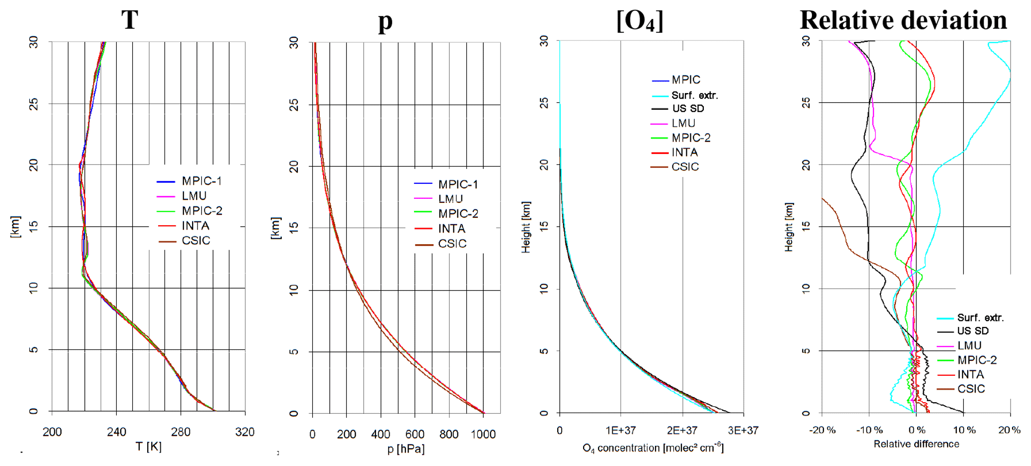
Figure 6Comparison of the vertical profiles of temperature, pressure and O4 concentration (expressed as the square of the O2 concentration) for 8 July, 11:00–19:00, extracted by the different groups. In the right panel the relative deviations in the O4 concentration are shown compared to the MPIC standard extraction. There, the profiles derived from the extrapolation from the surface values and the US standard atmosphere are also included.
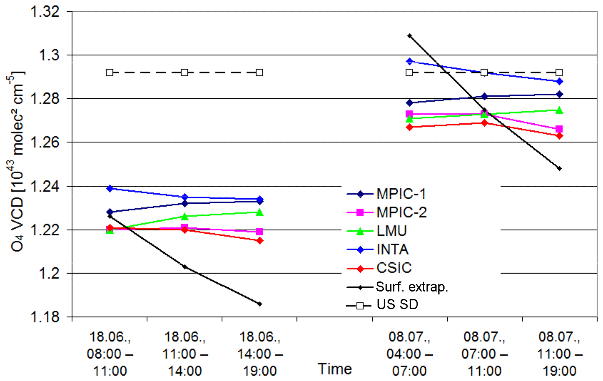
Figure 7Comparison of the O4 VCDs for the selected periods on both days calculated from the profiles extracted by the different groups. Also, the results for the profiles extrapolated from the surface values and the US standard atmosphere are shown.
Finally, the effects of individual extraction and integration procedures are investigated by comparing the results from different groups (see Fig. 6 and Fig. A5 in Appendix A3). Except for some extreme cases, the extracted temperatures typically differ by less than 3 K below 10 km. However, the deviations are typically larger for the profiles extrapolated from the surface values and in particular for the US standard atmosphere (up to >10 K below 10 km). The variations of the extracted pressure profiles are in general rather small (< 1 % below 10 km, except one obvious outlier). However, the deviations in the profiles extrapolated from the surface values, and especially the US standard atmosphere, are much larger (up to >5 % below 10 km). The resulting deviations in the O4 concentration from the different extractions are typically <3 % below 10 km (and up to >20 % above 10 km for the US standard atmosphere).
In Fig. 7 the O4 VCDs calculated for the O4 profiles extracted from the different groups and for the profiles extrapolated from the surface values and the US standard atmosphere are shown. The VCDs for the profiles extracted by the different groups agree within 2.5 %. The deviations in the profiles extrapolated from the surface values are only slightly larger (typically within 3 %) but show a large variability throughout the day, which is caused by the systematic increase in the surface temperature during the day (with temperature inversions in the morning on the 2 selected days). The deviations of the US standard atmosphere are up to 5 % (but can of course be larger for other seasons and locations; see also Ortega et al. (2016).
Ultimately, the accuracy with which O4 concentrations can be calculated is limited by the assumption that O4 (O2-O2) is pure collision-induced absorption. If the oxygen concentration profile is well known, the uncertainty due to bound O4 is smaller than 0.14 % in the Earth's atmosphere (Thalman and Volkamer, 2013).
Together with the uncertainties related to the input data sets, the total uncertainty of the O4 VCDs determined for both selected days is estimated at 3 %.
4.2 Uncertainties of the O4 (d)AMFs derived from radiative transfer simulations
The most important uncertainties of the simulated O4 (d)AMFs are related to the uncertainties of the input parameters used for the simulations, in particular the aerosol properties. Further uncertainties are caused by imperfections in the radiative transfer models. These sources of uncertainty are discussed and quantified in the following subsections.
4.2.1 Uncertainties of the O4 (d)AMFs caused by uncertainties of the input parameters
In this section the effect of the uncertainties of various input parameters on the O4 (d)AMFs is investigated. The general procedure is that the input parameters are varied individually and the corresponding changes in the O4 (d)AMFs compared to the standard settings are quantified.
First, the effect of the O4 profile shape is investigated. In contrast to the effect of the (absolute) profile shape on the O4 VCD (Sect. 4.1), here the effect of the relative profile shape on the O4 AMF is investigated. The O4 (d)AMFs simulated for the O4 profiles extracted by the different groups (and for those derived from the US standard atmosphere and the profiles extrapolated from the surface values; see Sect. 4.1) are compared to those for the MPIC O4 profiles (using the standard settings). The corresponding ratios are shown in Fig. A6 and Table A4 in Appendix A4. For the O4 profiles extracted by the different groups and for O4 profiles extrapolated from the surface values, small variations are found (typically <2 %). For the US standard atmosphere, larger deviations (up to 7 %) are derived.
Next the effect of the aerosol extinction profile is investigated. In this study, aerosol extinction profiles are derived from the combined ceilometer and sun photometer measurements (see Table 5). In short, the ceilometer measurements of the attenuated backscatter are scaled by the simultaneously measured AOD from the sun photometer to obtain the aerosol extinction profile. Also, the self-attenuation of the aerosol is taken into account. The different steps are illustrated in Fig. 8 and described in detail in Appendix A5. In the extraction procedure, several assumptions have to be made: first, the ceilometer profiles have to be extrapolated for altitudes below 180 m, for which the ceilometer is not sensitive. Furthermore, they have to be averaged over several hours and are in addition vertically smoothed (above 2 km) to minimise the rather large scatter. Finally, above 5 to 6 km (depending on the ceilometer profiles) the extinction is set to zero because of the further increasing scatter and the usually small extinctions. This assumption reflects a practical limitation of the ceilometer likely responsible for the larger variability in the profile shape aloft by different groups. Another assumption is that the Ångström exponent and the lidar ratio are independent of altitude, which is typically not strictly fulfilled (the lidar ratio describes the ratio between the extinction and backscatter probabilities of the molecules and aerosol particles).
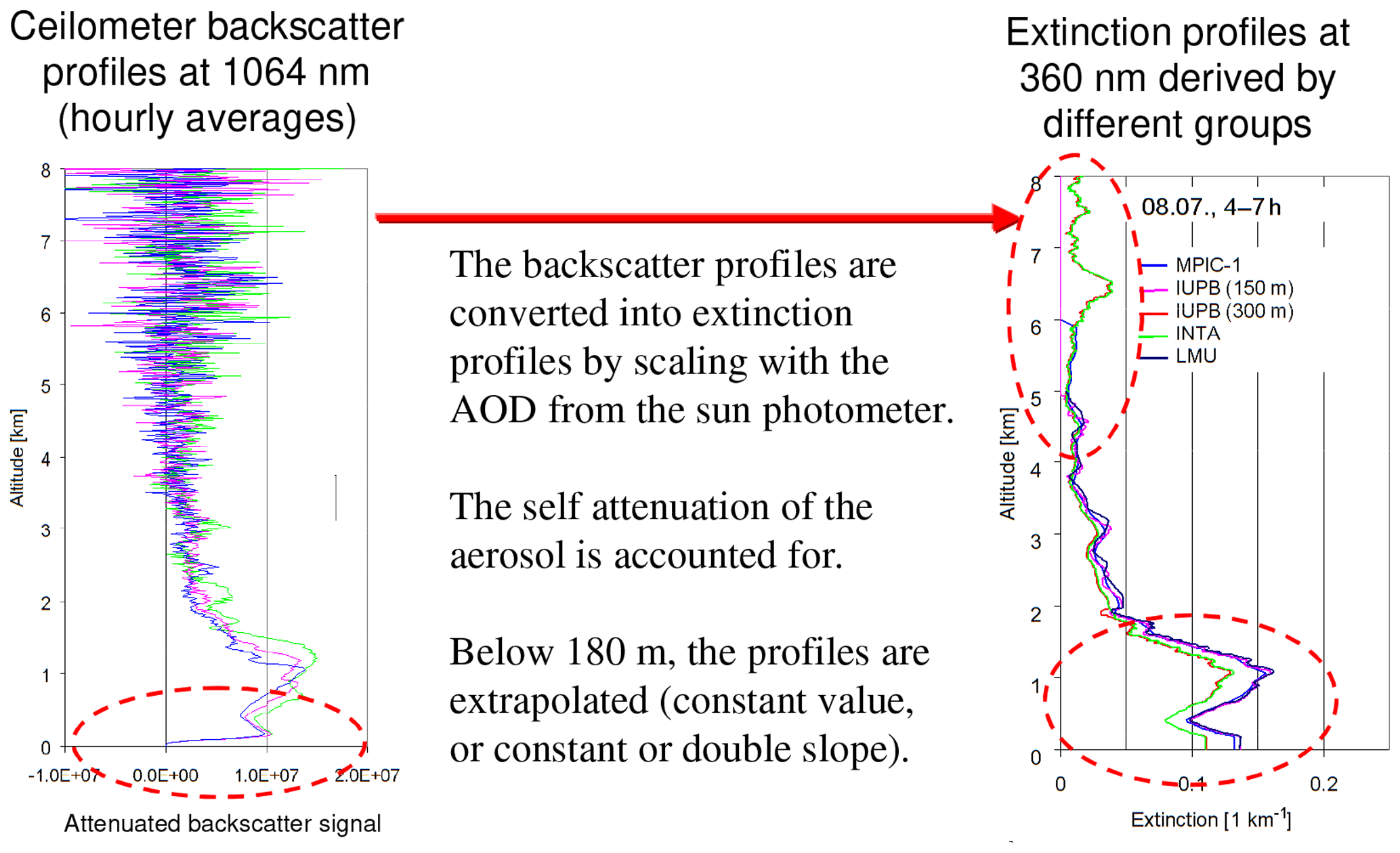
Figure 8Left: hourly averaged backscatter profiles from the ceilometer measurements for the period 04:00–07:00 on 8 July 2013. Below 180 m the values rapidly decrease to zero due to the missing overlap between the outgoing beam and the field of view of the telescope. Right: aerosol extinction profiles extracted by the different groups from the ceilometer profiles (assuming a constant extinction below 180 m). The red circles indicate the height intervals with the larger deviations (IUPB 150 m and IUPB 300 m indicate profile extractions with different widths of the smoothing kernels: Hanning windows of 150 and 300 m, respectively).
These uncertainties are quantified by sensitivity studies, in particular the effect of the extrapolation below 180 m and the altitude above which the aerosol extinction is set to zero. Other uncertainties, like the effect of the assumption of a constant lidar ratio, are more difficult to quantify without further information (see below). The effect of temporal averaging and smoothing is probably negligible for 8 July, because similar height profiles are found for all three periods of that day, but on 18 June the effect might be more important.
Figure 9 shows a comparison of the aerosol extinction profiles extracted by the different groups for the three periods on both days. Especially on 8 July, systematic differences are found. They are caused by the different altitudes above which the aerosol extinction is set to zero. In combination with the scaling of the profiles with the AOD obtained from the sun photometer, this also influences the extinction values close to the surface. Deviations up to 18 % are found for the first period of 8 July. These deviations also have an effect on the corresponding O4 (d)AMFs, where higher values are obtained for the profiles (INTA and IUPB 300 m) which were extracted for a larger altitude range (Fig. A7 and Table A5 in Appendix A4). Here it is interesting to note that these differences are not related to the direct effect of the aerosol extinction at high altitude but to the corresponding (via the scaling with the AOD) decrease in the aerosol extinction close to the surface. Larger deviations (up to 4 %) are found for 8 July, while the deviations on 18 June are within 3 %. This effect is further examined in Appendix A6.
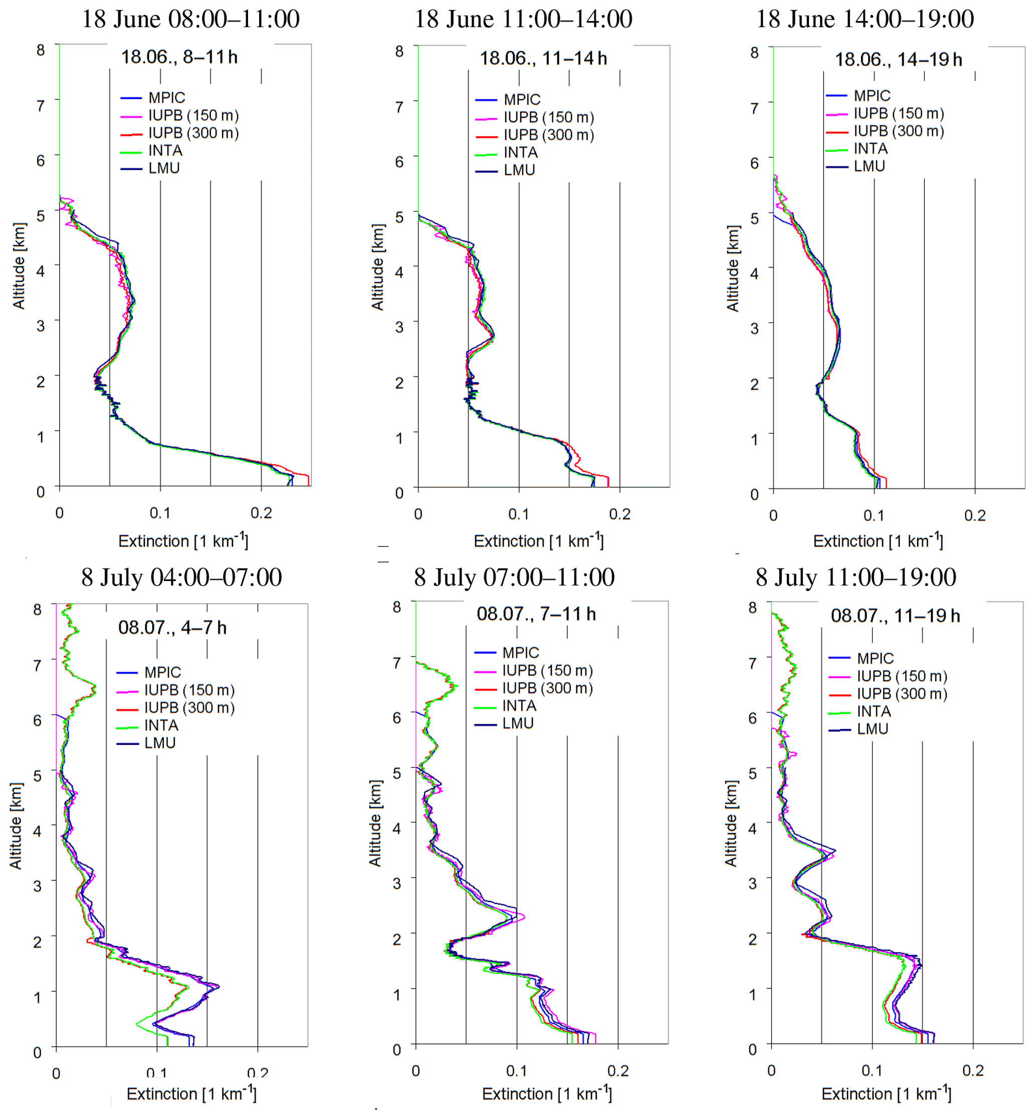
Figure 9Comparison of the aerosol extinction profiles extracted by the different groups for all three periods on both days.
In Fig. A8 and Table A6 in Appendix A4, the effect of the different extrapolations of the aerosol extinction profile below 180 m on the O4 (d)AMFs is quantified. Similar deviations (up to 5 %) are found for both days.
Finally, we investigated the effect of changing aerosol optical properties with altitude (changing lidar ratio). Such effects are particularly important if the wavelength of the ceilometer measurements (1064 nm) differs largely from that of the MAX-DOAS observations (360 nm). Based on the partitioning into fine- and coarse-mode aerosols (derived from the sun photometer observations) and the corresponding phase functions and optical depths, the sensitivity of the ceilometer to fine-mode aerosols was estimated (for details see Appendix A5). While for 18 June the contribution of the fine mode to the ceilometer signal is about 32 % on 8 July it is much larger (about 82 %). Thus, it can be concluded that the aerosol extinction profile derived from the ceilometer is largely representative of the fine-mode aerosols on that day. To investigate the effect of the remaining uncertainties, the shape of the aerosol extinction profile was further modified (for details see Appendix A5) while taking into account that the coarse aerosols are typically located at low altitudes. The corresponding repartitioning of the aerosol extinction profile led to a decrease in the aerosol extinction close to the surface, which is balanced by an increase at higher altitudes (see Fig. A34). The O4 dAMFs calculated for the modified profile are larger than those for the standard settings by about 17 % (for details see Appendix A5).
The effect of elevated aerosol layers (see Ortega et al., 2016) was further investigated by systematic sensitivity studies (Appendix A6). On both selected days enhanced aerosol extinction was found at elevated layers (Fig. 9). Compared to those reported by Ortega et al. (2016) the profiles extracted in this study reach up to even higher altitudes. For the investigation of the effect of changes in the aerosol extinction at different altitudes, the aerosol extinction profile on 8 July was subdivided into three layers (0–1.7, 1.7–4.9, 4.9–7 km), and the extinction in the individual layers was increased by +40 %. It was found that even a strong increase in the aerosol extinction at high altitudes by 40 % leads only to an increase in the O4 dAMFs of 7 %.
Also, the effect of horizontal gradients should be briefly discussed. For the selected periods of both days, the wind direction and wind speed were rather constant. On 18 June the wind direction was between 80 and 150∘ with respect to north, and the wind speed was about 2 m s−1. On 8 July the wind direction was between 70 and 90∘ (the wind came from almost the same direction at which the instruments were looking), and the wind speed was about 3 m s−1. During the 4 h of the selected period on 8 July, the air masses moved over a distance of about 40 km. During the 3 h of the selected period on 18 June, the air masses moved over a distance of about 20 km. These distances are larger than the distances to which the MAX-DOAS observations are sensitive (about 5–15 km). Since the AOD and the aerosol extinction profiles were also rather constant during both selected periods, we conclude that for the measurements considered here horizontal gradients can be neglected. It should also be noted that the discrepancies between measurements and simulations were simultaneously observed at all four azimuth directions.
In Fig. A9 and Table A7 in Appendix A4, the effect of different single scattering albedos (between 0.9 and 1) on the O4 (d)AMFs is quantified. The effect on the O4 (d)AMFs is up to 4 % on 18 June and up to 2 % on 8 July 2013.
The impact of the aerosol phase function is investigated in two ways: first, simulation results are compared for Henyey–Greenstein phase functions with different asymmetry parameters. The corresponding results are shown in Fig. A10 and Table A8 in Appendix A4. The differences in the O4 (d)AMFs for the different aerosol phase functions are rather strong: up to 3 % for the O4 AMFs and up to 8 % for the O4 dAMFs (larger uncertainties for the dAMFs are found because of the strong influence of the phase function on the 90∘ observations). Here it should be noted that the actual deviations from the true phase function might be even larger. In order to better estimate these uncertainties, simulations for phase functions derived from the sun photometer measurements based on Mie theory (in the following referred to as Mie phase functions) were also performed. A comparison of these Mie phase functions with the Henyey–Greenstein phase functions is shown in Fig. 10. Large differences, especially in the forward direction, are obvious. The O4 (d)AMFs for the Mie phase functions are compared to the standard simulations (using the HG phase function for an asymmetry parameter of 0.68) in Fig. A11 and Table A9 in Appendix A4. Again, rather large deviations are found, which are larger on 18 June (up to 9 %) than on 8 July (up to 5 %).

Figure 10Comparison of different aerosol phase functions used in the radiative transfer simulations. Panel (b) is a close-up of (a).
In Fig. A12 and Table A10 in Appendix A4, the effect of different surface albedos on the O4 (d)AMFs is quantified. For the considered variations (0.03 to 0.1) the changes in the O4 (d)AMFs are within 2 %.
4.2.2 Uncertainties of the O4 (d)AMFs caused by imperfections in the radiative transfer models
The radiative transfer models used in this study are well established and showed very good agreement in several intercomparison studies (e.g. Hendrick et al., 2006; Wagner et al., 2007; Lorente et al., 2017). Nevertheless, they are based on different methods and use different approximations (e.g. with respect to the Earth's sphericity). Thus, we compared the simulated O4 (d)AMFs for both days in order to estimate the uncertainties associated with these differences. In Fig. A13 and Table A11 (Appendix A4), the comparison results are shown. They agree within a few percent with slightly larger differences for 18 June (up to 6 %) than for 8 July (up to 3 %).
So far, all radiative transfer simulations were carried out without considering polarisation. Thus, in Fig. A14 and Table A12 in Appendix A4, the results with and without considering polarisation are compared. The corresponding differences are very small (<1 %).
4.2.3 Summary of uncertainties of the O4 AMF from radiative transfer simulations
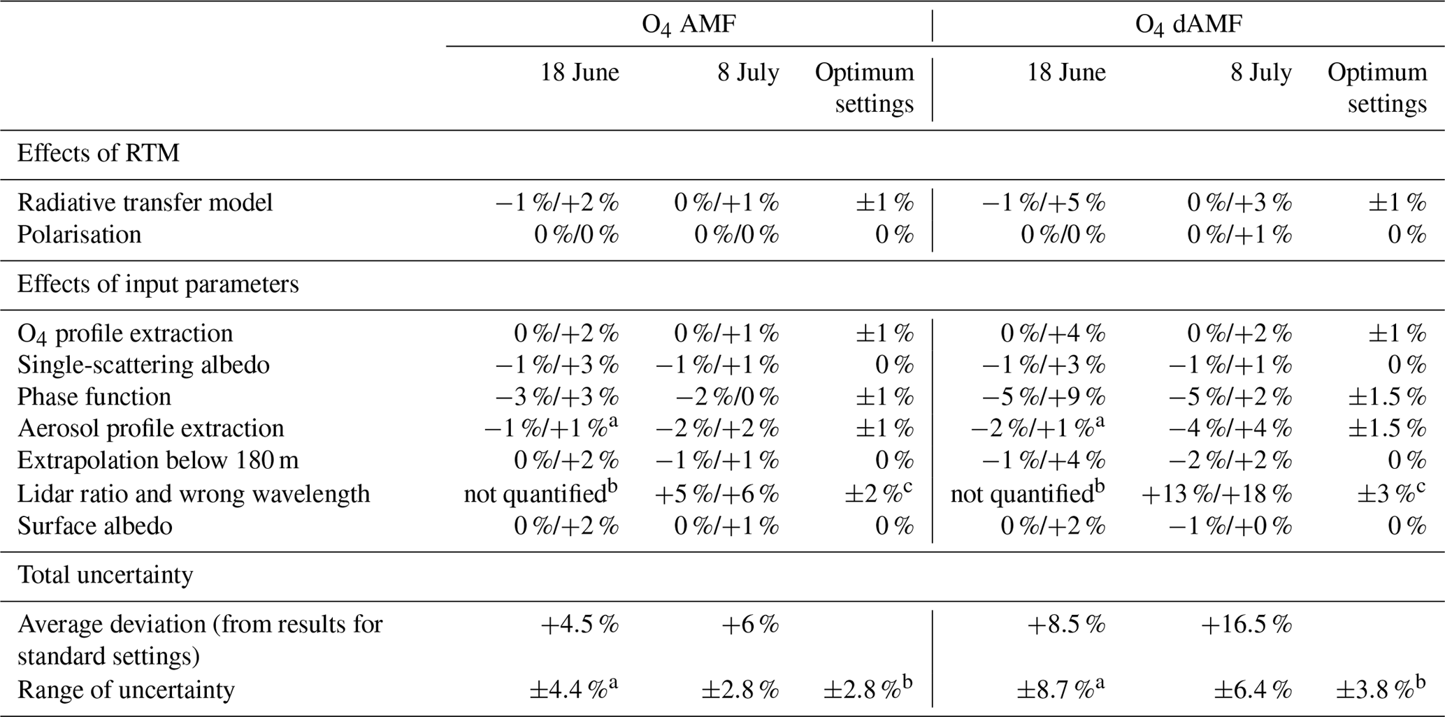
Table 9 presents an overview of the different sources of uncertainties of the simulated O4 (d)AMFs derived from the comparison of the results from different groups and the sensitivity studies. The uncertainties are expressed as relative deviations from the results for the standard settings (see Table 6) derived by MPIC using McArtim.
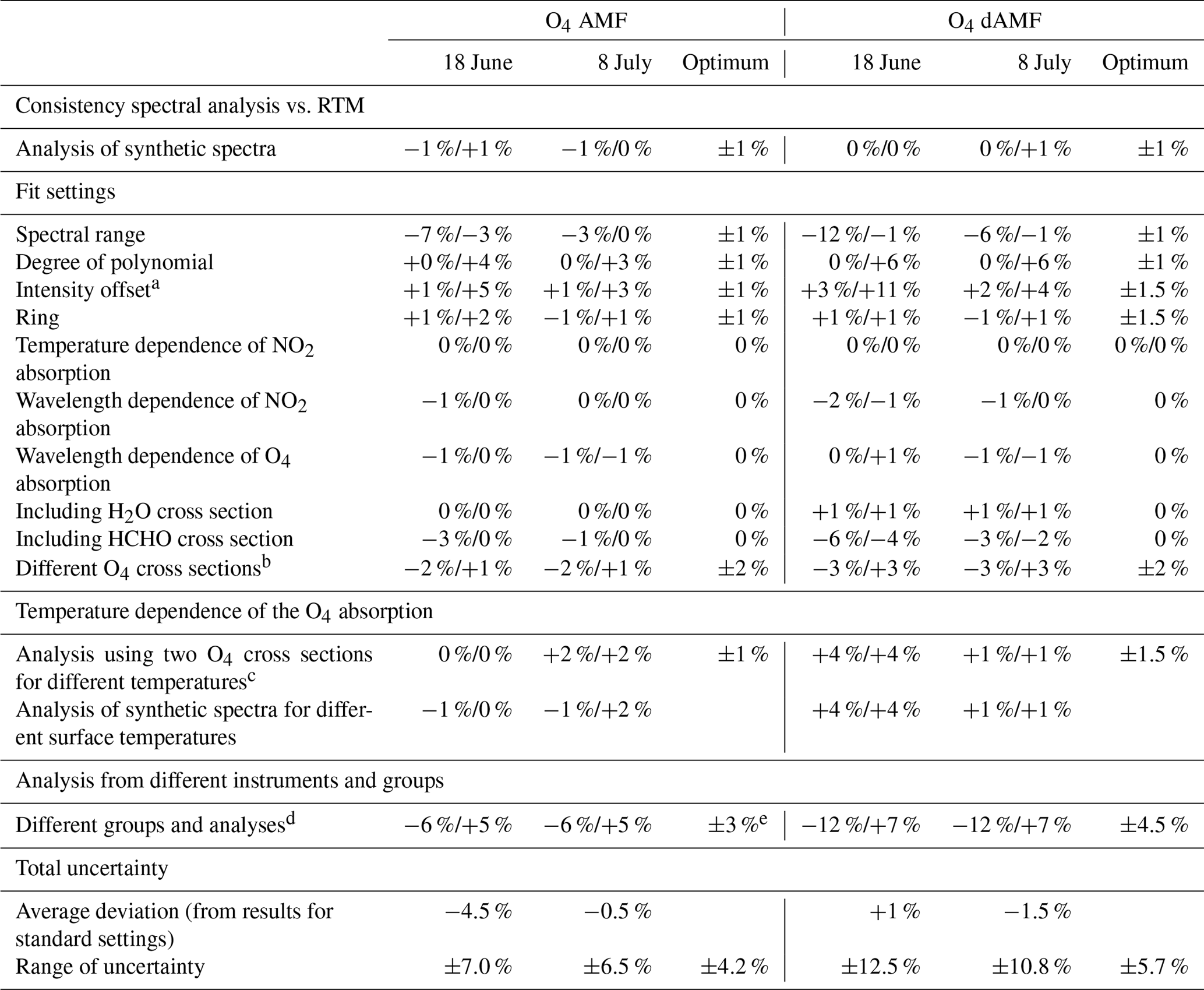
Table 9Summary of uncertainties of the simulated O4 (d)AMFs for the middle period of each selected day. The two numbers left and right of the slash indicate the minimum and maximum deviations. The columns with label “optimum” indicate the uncertainties which could be reached if the optimum information on the measurement conditions was available (e.g. height profiles of temperature, pressure and aerosol extinction as well as aerosol microphysical or optical properties).
a This uncertainty does not contain the contribution from variation of
aerosol properties with altitude; see text.
b Uncertainty was not assessed for 18 June 2013, because the contributions
from the coarse and fine mode at both wavelengths are very different (see Table A28). The uncertainty is thus much larger than on
8 July 2013.
c This was only the case if lidar profiles at the same wavelength and without gaps in the
troposphere were available.
In general, larger uncertainties are found for the O4 dAMFs compared to the O4 AMFs. This is expected because the uncertainties of the O4 dAMFs contain the uncertainties of two simulations (at 90∘ elevation and at low elevation). Another general finding is that the uncertainties on 18 June are larger than on 8 July. This finding is mainly related to the larger uncertainties due to the aerosol phase function, which has an especially strong forward peak on 18 June. Also, the uncertainties from the O4 profile extraction, the choice of the radiative transfer model and the extrapolation of the aerosol extinction below 180 m are larger on 18 June than on 8 July. These higher uncertainties are probably mainly related to the high aerosol extinction close to the surface on 18 June (see Sect. 5.1 and Appendices A2 and A5).
For the total uncertainties two values are given in Table 9: the average deviation is the sum of all systematic deviations of the individual uncertainties (the corresponding mean of the maximum and minimum values). The second quantity (the range of uncertainties) is calculated from half the individual uncertainty ranges by assuming that they are independent.
Finally, it should be noted that for some uncertainties (e.g. the effects of the surface albedo or the single-scattering albedo) the given numbers probably overestimate the true uncertainties, while for others, for example, the uncertainties related to the aerosol extinction profiles or the phase functions they possibly underestimate the true uncertainties (although reasonable assumptions were made). The two latter uncertainties are especially large for 18 June. The differences between the days are discussed in more detail in Sect. 5.
4.3 Uncertainties of the spectral analysis
The uncertainties of the spectral analysis are caused by different effects:
-
the specific settings of the spectral analysis like the fit window or the degree of the polynomial, particularly the effect of choosing different O4 cross sections as well as their temperature dependence;
-
the properties (and imperfections) of the MAX-DOAS instruments;
-
the effect of different analysis software and implementations;
-
the effect of the wavelength dependence of the AMF across the fit window.
These uncertainties are discussed and quantified in the following subsections.
4.3.1 Comparison of O4 (d)AMFs derived from the synthetic spectra with O4 (d)AMFs directly obtained from the radiative transfer simulations
Synthetic spectra for both selected days were simulated using the radiative transfer model SCIATRAN (for details see Sect. 2.4 and Table A3 in Appendix A1). While spectra for the whole day are simulated (for the viewing geometry see Table A2 in Appendix A1) it should be noted that the aerosol properties during the middle periods are also used for the whole day (to minimise the computational efforts). The spectra are analysed using the standard settings and the derived O4 (d)SCDs are converted to O4 (d)AMFs using Eq. (1). In addition to the spectra, O4 (d)AMFs at 360 nm are simulated directly by the RT models using exactly the same settings. These O4 (d)AMFs are used to test whether the spectral retrieval results are indeed representative of the simulated O4 (d)AMFs at 360 nm.
Spectra are simulated with and without considering the temperature dependence of the O4 cross section. Also, one version of synthetic spectra with added random noise is processed.

Figure 11Spectral analysis results for a real measurement from the MPIC instrument (left) and a synthetic spectrum with and without noise. Spectra are taken from 8 July 2013 at 11:26 (elevation angle=1∘). The derived O4 dSCD is shown above the individual plots.
First, the synthetic spectra are analysed using the standard settings (see Table 7). Examples of the O4 fits for synthetic (and measured) spectra are shown in Fig. 11. Here it is interesting to note that the ratios of the results for the measured and the simulated spectra are between 0.68 and 0.74, similarly to the ratio for the dAMFs on 8 July shown in Table 8.
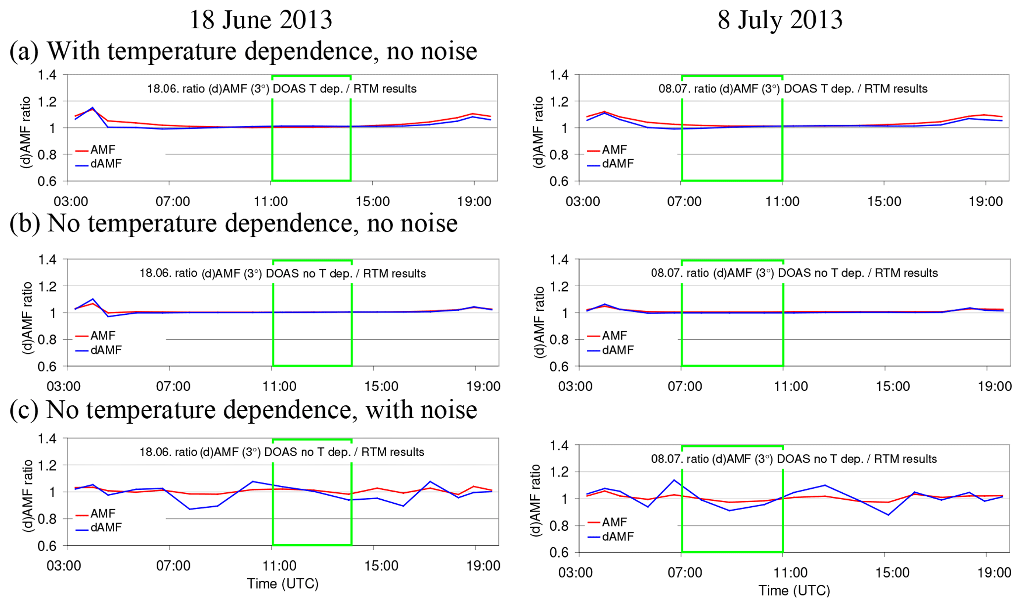
Figure 12Ratios of the O4 (d)AMFs derived from synthetic spectra vs. those obtained from radiative transfer simulations at 360 nm for both selected days.
In Fig. 12 the ratios of the O4 (d)AMFs derived from the synthetic spectra vs. those directly obtained from the radiative transfer simulations at 360 nm are shown. In panel (a) the results for synthetic spectra considering the temperature dependence of the O4 cross section are presented (without noise). Systematically enhanced ratios are found in the morning and evening, while for most of the day the ratios are close to unity. The higher values in the morning and evening are probably partly caused by the increased light paths through higher atmospheric layers (with lower temperatures) when the SZA is high. Interestingly, if the temperature dependence of the O4 cross section is not taken into account (Fig. 12b), slightly enhanced ratios during the morning and evening are still found, which can no longer be explained by the temperature dependence of the O4 cross section. Thus, we speculate that part of the enhanced values at high SZA are probably caused by the wavelength dependence of the O4 AMFs. Nevertheless, for most of the day the ratio is very close to unity, indicating that for SZA<75∘ the O4 (d)AMFs obtained from the spectral analysis are almost identical to the O4 (dAMFs) directly obtained from the radiative transfer simulations (at 360 nm).
In Fig. 12c results for spectra with added random noise (without consideration of the temperature dependence of the O4 cross section) are shown. On average similar results to those for the spectra without noise (Fig. 12b) are found but the results now show a large scatter. From these results and the spectral analyses (Fig. 11), we conclude that the noise added to the synthetic spectra overestimates that of the real measurements. For the sensitivity studies discussed in Sect. 4.3.2 only synthetic spectra without noise were used.
In Table A13 in Appendix A4 the average ratios for the middle period on each selected day are shown. They deviate from unity by up to 2 % indicating that the wavelength dependence of the O4 (d)AMF is negligible for the considered cases for SZA<75∘.
4.3.2 Sensitivity studies for different fit parameters
In this section the effect of the choice of several fit parameters on the derived O4 (d)AMFs is investigated using both measured and synthetic spectra. It should be noted that in the following only synthetic spectra without noise were used, because for the sensitivity studies we are interested in the systematic effects. Only one fit parameter is varied for each individual test, and the results are compared to those for the standard fit parameters (see Table 7).
First the fit window is varied. Besides the standard fit window (352 to 387 nm), which contains two O4 bands, two fit windows towards shorter wavelengths are also tested: 335–374 nm (including two O4 bands) and 345–374 nm (including one O4 band at 360 nm). The ratios of the derived O4 (d)AMFs vs. those for the standard analysis are shown in Fig. A15 and Table A14 in Appendix A2. On 18 June rather large deviations in the O4 (d)AMFs are found for both measured (−12 %) and synthetic spectra (−5 %) for the spectral range 335 to 374 nm. On 8 July the corresponding differences are smaller (−6 % and −2 % for measured and synthetic spectra, respectively). For the spectral range 345–374 nm, smaller differences of only up to 1 % are found for both days. The reason for the larger deviations on 18 June for the spectral range 335–374 nm is not clear. One possible reason could be the differences between the Ångström parameters (see Fig. 1) and phase functions (see Fig. 10).
In Fig. A16 and Table A15 the results for different degrees of the polynomial used in the spectral analysis are shown. For the measured spectra, systematically higher O4 (d)AMFs (up to 6 %) than for the standard analysis are found when using lower polynomial degrees. For the synthetic spectra the effect is smaller (<3 %).
In Fig. A17 and Table A16 the results for different intensity offsets are shown. Again, for the measured spectra systematically higher O4 (d)AMFs (up to 16 %) than for the standard analysis are found when reducing the order of the intensity offset, while for the synthetic spectra the effect is smaller (<3 %). Higher-order intensity offsets might compensate for wavelength-dependent offsets (e.g. spectral stray light), which can be important for real measurements, while the synthetic spectra do not contain such contributions. In Fig. A18 and Table A17 the results for spectral analyses with only one Ring spectrum are shown. In contrast to the standard analysis, which includes two Ring spectra (one for clear and one for cloudy sky; see Wagner et al., 2009), only the Ring spectrum for clear sky is used. For both selected days, only small deviations are found (within 2 %) compared to the standard analysis.
4.3.3 Sensitivity studies using different trace gas absorption cross sections
In this section the impact of different trace gas absorption cross sections on the derived O4 (d)AMFs is investigated.
In Fig. A19 and Table A18 the results for using two NO2 cross sections (294 and 220 K) compared to the standard analysis (using only a NO2 cross section for 294 K) are shown. The results are almost the same as for the standard analysis.
In Fig. A20 and Table A19 the results for using an additional wavelength-dependent NO2 cross section compared to the standard analysis (using only one NO2 cross section) are shown. The second NO2 cross section is calculated by multiplying the original cross section by wavelength (Puķīte et al., 2010). Again, only small deviations are found in the results from the standard analysis (1 % for the measured spectra and 2 % for the synthetic spectra).
In Fig. A21 and Table A20 results for using and additional wavelength-dependent O4 cross sections compared to the standard analysis (using only one O4 cross section) are shown. The second O4 cross section is calculated like for NO2 but an orthogonalisation with respect to the original O4 cross section (at 360 nm) is also performed. The derived O4 (d)AMFs are almost identical to those from the standard analysis (within 1 %).
For the spectral retrieval of HONO in a similar spectral range, a significant impact of water vapour absorption, around 363 nm, was found in Wang et al. (2017a) and Lampel et al. (2017). In Fig. A22 and Table A21 the O4 results for including a H2O cross section (Polyansky et al., 2018) compared to the standard analysis (using no H2O cross section) are shown. The results are almost identical to those from the standard analysis (within 1 %).
In Fig. A23 and Table A22 the results for including a HCHO cross section compared to the standard analysis (using no HCHO cross section) are shown. Especially for 18 June a large systematic effect is found: the O4 dAMFs are smaller than for the standard analysis for measured and synthetic spectra by 4 % and 6 %, respectively. On 8 July the underestimation is smaller (2 % and 3 % for measured and synthetic spectra).
4.3.4 Effect of using different O4 cross sections
In Fig. A24 and Table A23 the results for different O4 cross sections are compared to the standard analysis (using the Thalman O4 cross section). The results for both days are almost identical. For the real measurements, the derived O4 dAMFs using the Hermans and Greenblatt cross sections are 3 % smaller and 8 % larger than those for the standard analysis, respectively. However, if the Greenblatt O4 cross section is allowed to shift during the spectral analysis, the overestimation can be largely reduced to only +3 %. This confirms findings from earlier studies (e.g. Pinardi et al., 2013) that the wavelength calibration of the original data sets is not very accurate.
For the synthetic spectra slightly different results to those for the real measurements are found for the Hermans O4 cross section. The reason for these differences is not clear. However, here it should be noted that the temperature-dependent O4 absorption in the synthetic spectra does probably not exactly represent the true atmospheric O4 absorption.
4.3.5 Effect of the temperature dependence of the O4 cross section
The new set of O4 cross sections provided by Thalman and Volkamer (2013) allows the temperature dependence of the atmospheric O4 absorptions to be investigated in detail. They provide O4 cross sections measured at five temperatures (203, 233, 253, 273, 293 K) covering the range of temperatures relevant for atmospheric applications. Using these cross sections, the effect of the temperature dependence of the O4 absorptions is investigated in two ways:
-
In a first test, synthetic spectra are simulated for different surface temperatures assuming a fixed lapse rate. These spectra are then analysed using the O4 cross section for 293 K (which is usually used for the spectral analysis of O4). From this study the magnitude of the effect of the temperature dependence of the O4 cross section on MAX-DOAS measurements can be quantified.
-
In a second test, measured and synthetic spectra for both selected days are analysed with O4 cross sections for different temperatures. From this study it can be seen to which degree the temperature dependence of the O4 cross section can be already corrected during the spectral analysis (if two O4 cross sections are used simultaneously).
For the first study, MAX-DOAS spectra are simulated in a simplified way:
-
Atmospheric temperature profiles are constructed for surface temperatures between 220 and 310 K in steps of 10 K assuming a fixed lapse rate of .
-
For each altitude layer (vertical extension: 20 m below 500 m, 100 m between 500 m and 2 km, 200 m between 2 and 12 km, 1 km above) the O4 concentrations (calculated from the US standard atmosphere) are multiplied by the corresponding differential box AMFs calculated for typical atmospheric conditions and viewing geometries (see Fig. A25 in Appendix A4).
-
High-resolution absorption spectra are calculated by applying the Beer–Lambert law for each height layer using the O4 cross section of the respective temperature (interpolated between the two adjacent temperatures of the Thalman and Volkamer data set).
-
The derived high-resolution spectra are convolved with the instrument slit function (FWHM of 0.6 nm).
-
The logarithm of the ratio of the spectra for the low elevation and zenith is calculated and analysed using the O4 cross section for 293 K.
-
The derived O4 dAMFs are divided by the corresponding dAMFs directly obtained from the radiative transfer simulations.
These calculated ratios as a function of the surface temperature are shown in Fig. 13. A strong and systematic dependence on the surface temperature is found (a 15 % change for a change in the surface temperature between 240 and 310 K). However, except for measurements at polar regions, the deviations are usually small. Since for both selected days the temperatures were rather high (indicated by the two coloured horizontal bars in the figure), the effect of the temperature dependence of the O4 absorption for the middle period of each day is very small (−1 % to −2 % for 18 June and 0 % to +1 % on 8 July). It should be noted that the results shown in Fig. 13 are obtained for generalised settings of the radiative transfer simulations. Thus, it is recommended that future studies should investigate the effect of the temperature dependence in more detail and using the exact viewing geometry for individual observations. However, since the temperatures on both selected days were rather high, for this study the simplifications of the radiative transfer simulations have no strong influence on the derived results.
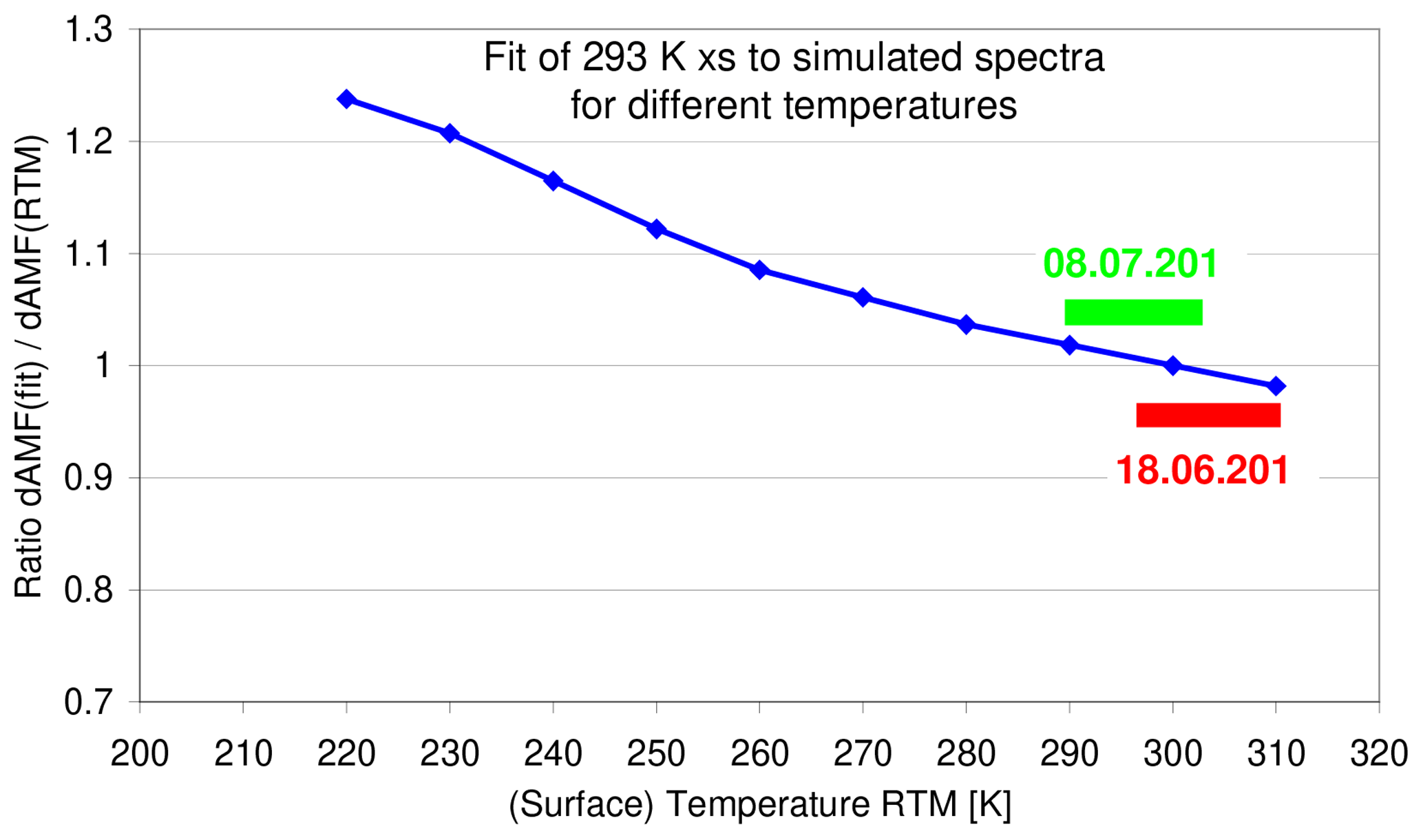
Figure 13Ratios of the O4 dAMF obtained from simulated spectra for different surface temperatures by the corresponding O4 dAMFs derived from radiative transfer simulations. The results represent MAX-DOAS observations at low-elevation angles (2 to 3∘).
In the second test the measured and synthetic spectra are analysed using O4 cross sections for different temperatures. The corresponding results are shown in Fig. A26 and Table A24.
If only the O4 cross section at low temperature (203 K) is used, the derived O4 AMFs and dAMFs are about 16 % and 30 % smaller than for the standard analysis (using the O4 cross section for 293 K). These results are consistently obtained for the measured and synthetic spectra. If, however, two O4 cross sections (for 203 and 293 K) are simultaneously included in the analysis, different results are obtained for the measured and synthetic spectra: for the measured spectra the derived O4 (d)AMFs agree within 4 % with those from the standard analysis. In contrast, for the synthetic spectra, the derived O4 (d)AMFs are systematically smaller (by about 6 % to 18 %). This finding was not expected, because exactly the same cross sections were used for both the simulation and the analysis of the synthetic spectra. Detailed investigations (see Appendix A4) led to the conclusion that there is a slight inconsistency in the temperature dependence of the O4 cross sections from Thalman and Volkamer (2013): the ratio of the peak values of the cross section at 360 and 380 nm changes in a non-continuous way between 253 and 233 K (see Fig. A27 in Appendix A4); see also Fig. S2 (values for 380 nm) in the supplementary material of Thalman and Volkamer (2013). The reason for this inconsistency is currently not known. If these two O4 bands are included in the spectral analysis (as for the standard settings), the convergence of the spectral analysis strongly depends on the ability to fit both O4 bands well. Thus, the fit results for both O4 cross sections are mainly determined by the relative strengths of both O4 bands (see Fig. A27 in Appendix A4). If instead a smaller wavelength range is used containing only one absorption band (345–374 nm), the derived O4 (d)AMFs are in rather good agreement with the results of the analysis (using only the O4 cross section for 293 K); see Table A25 in Appendix A4. In that case, the convergence of the fit mainly depends on the temperature dependence of the line width. It should be noted that the non-continuous temperature dependence of the O4 absorption cross section only affects the analysis of the synthetic spectra, because for the simulation of the spectra all O4 cross sections for temperatures between 233 and 293 K were used. For the measured spectra, no problems are found, because in the spectral analysis only the O4 cross sections for 233 and 293 K were used.
In Fig. A28 in Appendix A4 the ratios of both fit coefficients (for 203 and 293 K) are shown, as well as the derived effective temperatures for the analyses of measured and synthetic spectra. For the measured spectra the ratios are close to zero and the derived temperatures are close to 300 K most of the time (except in early morning and evening), because the effective atmospheric temperature for both days is close to the temperature of the high temperature O4 cross section (293 K) (see Fig. 13). Similar results (at least around noon) are also obtained for the synthetic spectra if the narrow spectral range (345–374 nm) is used. For the standard fit range (including two O4 bands), however, the ratios are much higher, again indicating the effect of the inconsistency of the temperature dependence of the O4 cross sections (see Fig. A27 in Appendix A4).
4.3.6 Results from different instruments and analyses by different groups
In this section the effects of using measurements from different instruments and having these spectra analysed by different groups are investigated. For that purpose three different procedures are followed: first, MPIC spectra are analysed by other groups; second, the spectra from other instruments are analysed by MPIC; third, the spectra from non-MPIC instruments are analysed by the respective group.
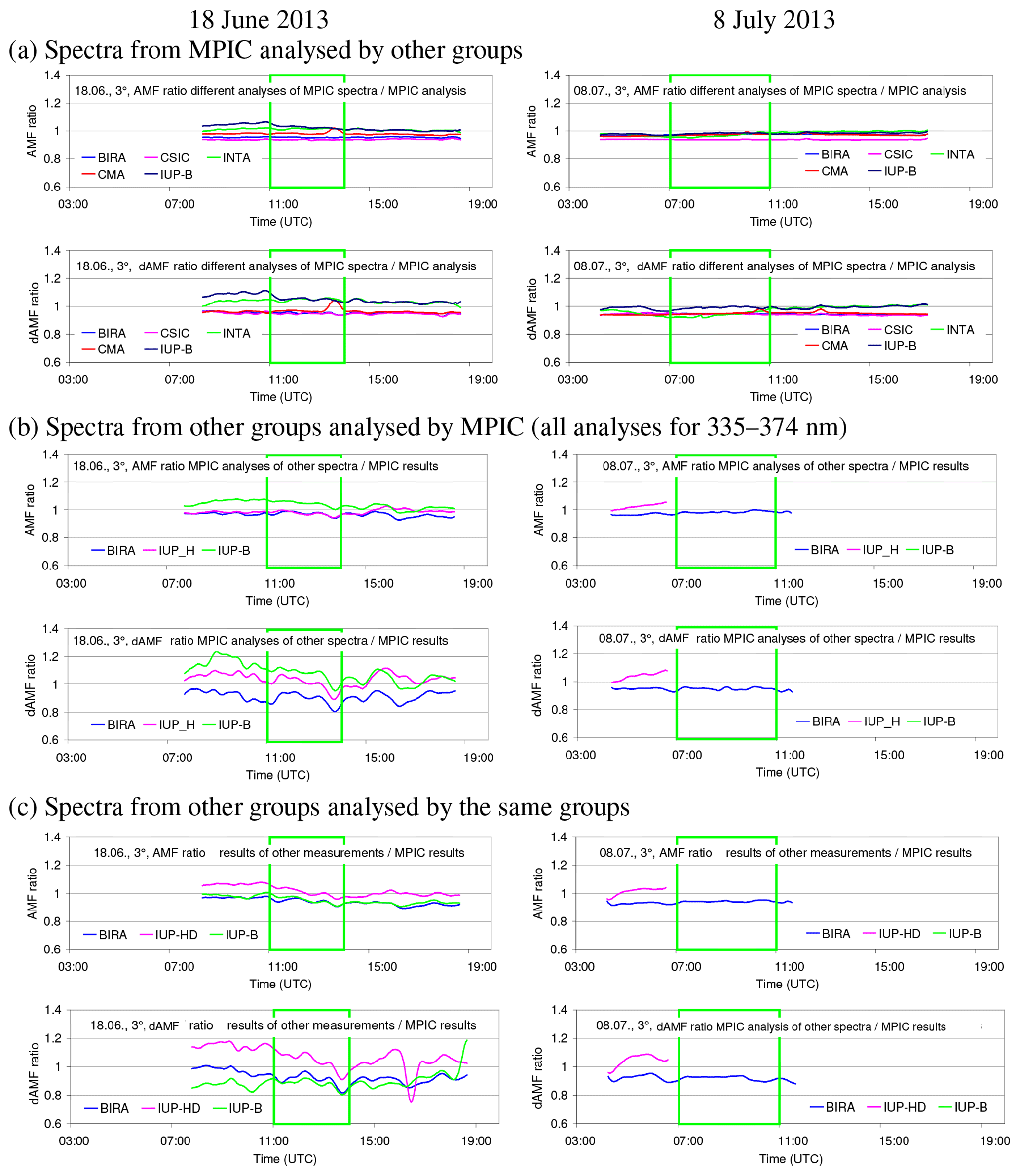
Figure 14(a) Ratios of the O4 (d)AMFs derived from MPIC spectra when analysed by other groups vs. those analysed by MPIC for both selected days. (b) Ratios of the O4 (d)AMFs derived from spectra measured by other groups but analysed by MPIC vs. those for the MPIC instrument analysed by MPIC (using the spectral range 335–374 nm for all instruments). (c) Ratios of the O4 (d)AMFs derived from spectra measured and analysed by other groups (using different wavelength ranges and settings) vs. those for the MPIC instrument analysed by MPIC.
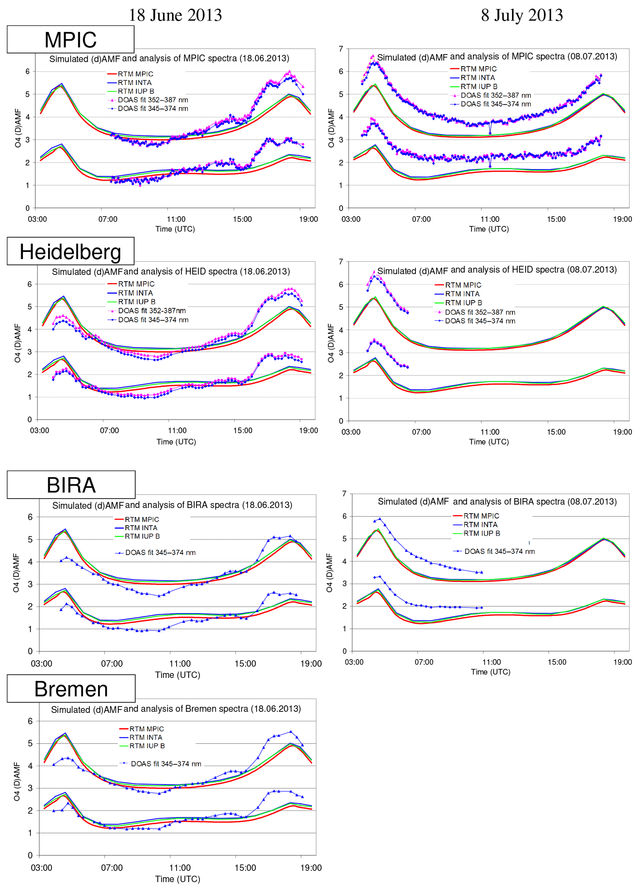
Figure 15Comparison of measured and simulated O4 (d)AMFs for both selected days. Measurements are from four different instruments but are analysed by MPIC using the standard settings (see Table 7). Simulations are performed by three different groups using Mie phase functions and otherwise the standard settings (see Table 6).
In Fig. 14a and Table A25 (in Appendix A4) the comparison results of the analysis of MPIC spectra by other groups vs. the analysis of MPIC spectra by MPIC are shown. Especially for 18 June, rather large differences (between −6 %/+5 %) to the MPIC standard analysis are found. Interestingly the largest differences are found in the morning when the aerosol extinction close to the surface was strongest. On 8 July smaller differences (between −6 % and −1 %) are found.
In Fig. 14b and Table A25 (in Appendix A4) the comparison results of the analysis of spectra from other instruments by MPIC vs. the analysis of MPIC spectra by MPIC are shown. For this comparison all analyses are performed in the spectral range 335–374 nm, because the standard spectral range (352–387 nm) is not covered by all instruments. Again, the largest differences are found for 18 June (up to ±11 %). For 8 July the differences reach up to ±6 %, but for this day only a few measurements in the morning are available.
In Fig. 14c and Table A25 (in Appendix A4) the comparison results of the analysis of spectra from other instruments by the respective group vs. the MPIC analysis by MPIC (standard analysis) is shown. From this exercise the combined effects of different instrumental properties and retrievals can be estimated. Interestingly, the observed differences are only slightly larger than those for the analysis of the spectra from the different instruments by MPIC (Fig. 14b). This indicates that the largest uncertainties are related to the differences in the different instruments and not to the settings and implementations of the different retrievals. For the middle period of 18 June the uncertainties are within 12 %. This range is also assumed for 8 July. Here it is interesting to note that the derived uncertainties of the spectral analysis are probably not representative of most recent measurement campaigns. For example, during the CINDI-2 campaign (http://www.tropomi.eu/data-products/cindi-2, last access: 29 April 2019) the deviations in the O4 spectral analysis results were much smaller than for the selected days during the MAD-CAT campaign (Kreher et al., 2019). A summary of the comparison of the measurements from different instruments and radiative transfer simulations using different models is given in Fig. 15.
4.3.7 Summary of uncertainties of the O4 AMF from the spectral analysis
Table 10 presents an overview of the different sources of uncertainty of the measured O4 (d)AMFs obtained in the previous subsections. The uncertainties are expressed as relative deviations from the results for the standard settings (see Table 7) derived by MPIC from spectra of the MPIC instrument.
Table 10Summary of uncertainties of the measured O4 (d)AMFs for the middle period of each selected day. The two numbers left and right of the slash indicate the minimum and maximum deviations. The columns labelled “optimum” indicate the uncertainties which could be reached if optimum instrumental performance was ensured and optimum cross section was available.
a Here the case “no offset” is not considered.
b Here the case of the non-shifted Greenblatt O4 cross
section is not considered.
c Here only the results for the measured spectra in the
spectral range 352–387 nm are considered (temperatures on 18 June:
27–31 ∘C; 8 July: 20–30 ∘C).
d The results for 18 June are also taken for 8 July due to
the lack of measurements on 8 July.
e See Kreher et al. (2019).
Like for the simulation results, in general, larger uncertainties are found for the O4 dAMFs compared to the O4 AMFs. This is expected because the uncertainties of the O4 dAMFs contain the uncertainties of two analyses (at 90∘ elevation and at low elevation). Also, the uncertainties on 18 June are again larger than on 8 July. This finding was not expected but is possibly related to the higher trace gas abundances (see Fig. 1 and Table A3 in Appendix A1) and the higher aerosol extinction close to the surface on 18 June.
Another interesting finding is that the uncertainties of the spectral analysis of O4 are dominated by the effect of instrumental properties up to ±12 % in the morning of 18 June. Further important uncertainties are associated with the choice of the wavelength range, the degree of the polynomial and the intensity offset. In contrast, the exact choices of the trace gas cross sections (including their wavelength- and temperature dependencies) play only a minor role (up to a few percent). Excellent agreement (within ±1 %) is found in particular for the O4 analysis of the synthetic spectra using the standard settings and the directly simulated O4 (d)AMFs at 360 nm. This indicates that the O4 (d)AMFs retrieved in the wavelength range 352–387 nm are indeed representative of radiative transfer simulations at 360 nm.
As for the uncertainties of the simulated O4 (d)AMFs, the uncertainties of the spectral analysis are also split into a systematic and a random term: the systematic deviations in the O4 dAMFs from those of the standard settings are about +1 % and −1.5 % for 18 June and 8 July, respectively. The range of uncertainty is calculated from the uncertainty ranges of the different contributions by assuming that they are all independent. The random uncertainty ranges for 18 June and 8 July are calculated as ±12.5 % and ±10.8 %, respectively.
4.4 Recommendations derived from the sensitivity studies
In this section a short summary of the most important findings from the sensitivity studies is given.
-
Temperature and pressure profiles.
Temperature and pressure profiles from sondes or model data should be used if available. Alternatively, temperature and pressure profiles extrapolated from surface measurements could be used. Typical uncertainties of the O4 VCD derived from such profiles are still <2 %. For high temperatures (<20 ∘C) the atmospheric humidity should be considered. If no measurements are available, prescribed profiles can be used, e.g. from the US standard atmosphere or climatologies of temperature and pressure profiles. However, depending on location and season the uncertainties of the resulting O4 VCD can be rather large (see also Ortega et al., 2016).
-
Integration of the O4 VCD
The integration should be performed on a vertical grid with at least 100 m resolution up to an altitude of 30 km. The surface altitude should be taken into account with an accuracy of at least 20 m.
-
Measurements and spectral analysis.
Instruments should have a small field of view (≤1∘), an accurate elevation calibration (better than 0.5∘) and a small and preferably well-characterised stray light level. For the data analysis the standard settings provided in Table 7 should be used. From the analysis of synthetic spectra it was found that the results for these settings are consistent with simulated O4 (d)AMFs within 1 %.
-
Information on aerosols.
Aerosol profiles should be obtained from lidar or ceilometers using similar wavelengths to the MAX-DOAS measurements if available (see e.g. Ortega et al., 2016). Preferred lidar types are High Spectral Resolution Lidar (HSRL) or Raman lidar, which directly provide profiles of aerosol extinction and thus need no assumptions on the lidar ratio. They should also have high signal-to-noise ratios and a shallow blind region at the surface in order to cover a large altitude range. Information on aerosol optical properties and size distributions from sun photometers or in situ measurements should be used.
-
RTM simulations.
Radiative transfer models should use Mie phase functions and aerosol single-scattering albedo, e.g. derived from sun photometer observations. The consideration of polarisation and rotational Raman scattering is not necessary.
In summary, if the optimised settings described above are used, the uncertainties of the radiative transfer simulations and spectral analysis can be largely reduced: the uncertainties of the O4 dAMFs related to radiative transfer simulations can be reduced from about ±8 % as in this study to about ±4 %; those related to the spectral analysis can be reduced from about ±10 % to about ±6 %.
Preferred scenarios for future studies
In addition to the recommendations given above, future campaigns should aim to cover different meteorological conditions (e.g. low temperatures), viewing geometries (e.g. low SZA), surface albedos (e.g. snow and ice) and wavelengths (e.g. 477, 577 and 630 nm). Also, different aerosol scenarios including those with low AOD should be covered. MAX-DOAS measurements should be performed by at least 2 instruments but preferably more. In order to minimise the effects of instrumental properties, the instruments should be well calibrated and should have low stray light levels. Measurements obtained during the CINDI-2 campaign are probably well suited for a similar study.
The comparison results for both days are different: on 18 June (except in the evening) measurements and simulations agree within uncertainties (the ratio of simulated and measured O4 dAMFs for the middle period of that day is 1.01±0.16). In contrast, on 8 July, measurements and simulations significantly disagree: taking into account the uncertainties of the VCD calculation (3 %), the radiative transfer simulations ( %) and the spectral analysis ( %) for the middle period of that day results in a ratio of simulated and measured O4 dAMFs of 0.82±0.10, which differs significantly from unity.
5.1 Important differences between the days
On both selected days similar aerosol AODs were measured. Also, the diurnal variation of the SZA was similar because of the proximity to the summer solstice. However, many differences are also found for the 2 selected days, which are discussed below.
-
Temperature, pressure and wind.
On 18 June surface pressure was lower by about 13 hPa and surface temperature was higher by about 7 K than on 8 July, respectively. These differences were explicitly taken into account in the calculation of the O4 profiles or VCDs, the radiative transfer simulations and the interpretation of the spectral analyses. Thus, they are very unlikely to explain the different comparison results on the 2 selected days.
On both days, wind was mainly blowing from east–north-east, but on 18 June it was blowing from the west before about 08:00 and after 20:00 UTC. Wind speeds were lower on 18 June (between 1 and 2 m s−1) than on 8 July (between 1 and 3 m s−1).
-
Aerosol properties.
The in situ aerosol measurements show very different abundances and properties of aerosols close to the ground for the selected days. On 18 June much higher concentrations of larger aerosol particles are found, which cannot be measured by the ceilometer due to the blindness for the lowest 180 m. Thus, it can be concluded that the enhanced aerosol concentration on 18 June is confined to a shallow layer at the surface. In general the aerosol concentrations close to the surface are more variable on 18 June than on 8 July. The high aerosol concentrations close to the surface probably also affect the lidar ratio, which is thus probably more variable on 18 June. Similarly, the phase function derived from the sun photometer (for the integrated aerosol profile) is also probably less representative of the low-elevation angles on 18 June because different aerosol size distributions probably existed at different altitudes. Finally, the Ångström parameter derived from AERONET observations is different for both days, especially for large wavelengths, which is in qualitative agreement with the higher in situ aerosol concentrations of large particles on 18 June. Also, a larger forward peak of the derived aerosol phase function is found for 18 June. Both effects probably cause larger uncertainties on 18 June.
-
Spectral analysis.
Larger uncertainties of the spectral analysis are found for 18 June compared to 8 July. This finding was surprising but was also partly reproduced by the analysis of the synthetic spectra. One possible explanation is the smaller wavelength dependence of aerosol scattering at low altitudes on 18 June, which mainly affects measurements at low-elevation angles. When analysed vs. a zenith reference, for which the broadband wavelength dependency is much stronger (because of the larger contribution from Rayleigh scattering), larger deviations can be expected (e.g. because of differences in instrumental stray light, or the different detector saturation levels). On 18 June higher (about doubled) NO2 and HCHO concentrations are also present compared to 8 July, possibly leading to increased spectral interferences with the O4 absorption, but this effect is expected to be small.
5.2 Which conditions would be needed to bring measurements and simulations on 8 July into agreement
This section tentatively describes possible (although generally unrealistic) changes in the atmospheric scenario, the instrument properties or the input parameters, which could bring measurements and simulations on 8 July into agreement. If, for example, the whole aerosol extinction profile was scaled by 0.65, the corresponding O4 dAMFs would almost perfectly match the measured ones.
A similarly good agreement could also be achieved if about 27 % of the total AOD was shifted from low layers (below 1.68 km) to high layers (above 4.9 km; see Appendix A6). However, in this scenario, about 73 % of the total aerosol extinction would be above 1.68 km. Such a scenario would not be in agreement with the AERONET inversion products and would also lead to an underestimation of the diurnal variation of the O4 AMFs measured in zenith direction.
Also, horizontal gradients of the aerosol extinction could in principle explain the discrepancy. While we are not able to quantify them, they surely would have to be of the order of several tens of percent per 10 km. Such persistent horizontal gradients are not supported by the almost constant AOD during the day (and also by the consistent aerosol in situ observations at the different sites). Also, the mismatch between measurements and simulations that is found for all azimuth angles indicates that horizontal gradients can not explain the observed discrepancies.
Another possibility would be aerosol phase functions with very high asymmetry parameters (≫0.75). Also, systematic errors of the O4 cross section could explain the observed discrepancies. Finally, an overcorrection of spectrograph stray light (or any other intensity offset) could explain the discrepancies. However, a rather high overcorrection (by about 20 %) would be needed, which is probably unrealistic.
We compared MAX-DOAS observations of the atmospheric O4 absorption with corresponding radiative transfer simulations for 2 mainly cloud-free days during the MAD-CAT campaign. A large part of this study is dedicated to the extraction of input information for the radiative transfer simulations and the quantification of the associated uncertainties of the radiative transfer simulations and spectral retrievals. An important result from the sensitivity studies is that the O4 results derived from the analysis of synthetic spectra using the standard settings are consistent with the simulated O4 air mass factors within 1 %. Also, recommendations for the settings of the radiative transfer simulations, in particular on the extraction of aerosol and O4 profiles are given. Another important result is that the extent and quality of the aerosol data sets is crucial to constrain the radiative transfer simulations. For example, it is recommended that lidar instruments are operated at wavelengths close to those of the MAX-DOAS measurements (see Ortega et al., 2016) and have a small sensitivity gap close to the surface. Further aerosol properties (e.g. size distributions, phase functions) should be available from sun photometer and/or in situ measurements. If such aerosol data are available the corresponding uncertainties of the radiative transfer simulations could be largely reduced to about ±5 %. Similar uncertainties can also be expected for optimum instrument operations and data analyses.
The comparison results for both days are different: on 18 June (except in the evening) measurements and simulations agree within uncertainties (the ratio of simulated and measured O4 dAMFs for the middle period of that day is 1.01±0.16). In contrast, on 8 July measurements and simulations significantly disagree: taking into account the uncertainties of the VCD calculation (3 %), the radiative transfer simulations ( %) and the spectral analysis ( %) for the middle period of that day results in a ratio of simulated and measured O4 dAMFs of 0.82±0.10, which differs significantly from unity. So far no plausible explanation for the observed discrepancies on 8 July was found.
However, as long as the reason for this deviation is not understood, it is unclear how representative these findings are for other measurements (e.g. from other platforms, at other locations or seasons, for other aerosol loads and other wavelengths). Thus, further studies spanning a larger variety of measurement conditions and including other wavelengths are recommended. The MAX-DOAS measurements collected during the recent CINDI-2 campaign are probably well suited for that purpose.
The data used in this study are available at: http://joseba.mpch-mainz.mpg.de/Comparison.htm (last access: 29 April 2019).
A1 Settings used for the simulation of synthetic spectra
Table A1Vertical resolution used in radiative transfer simulations for different altitude ranges.
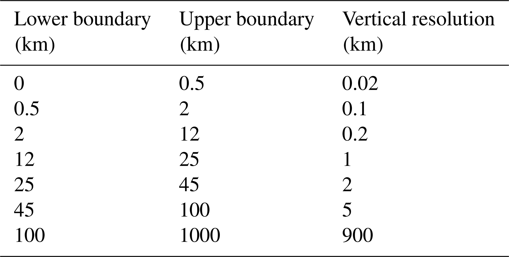
Table A2Dependence of SZA and RAZI on time (UTC) for the standard viewing direction (51∘ with respect to north).
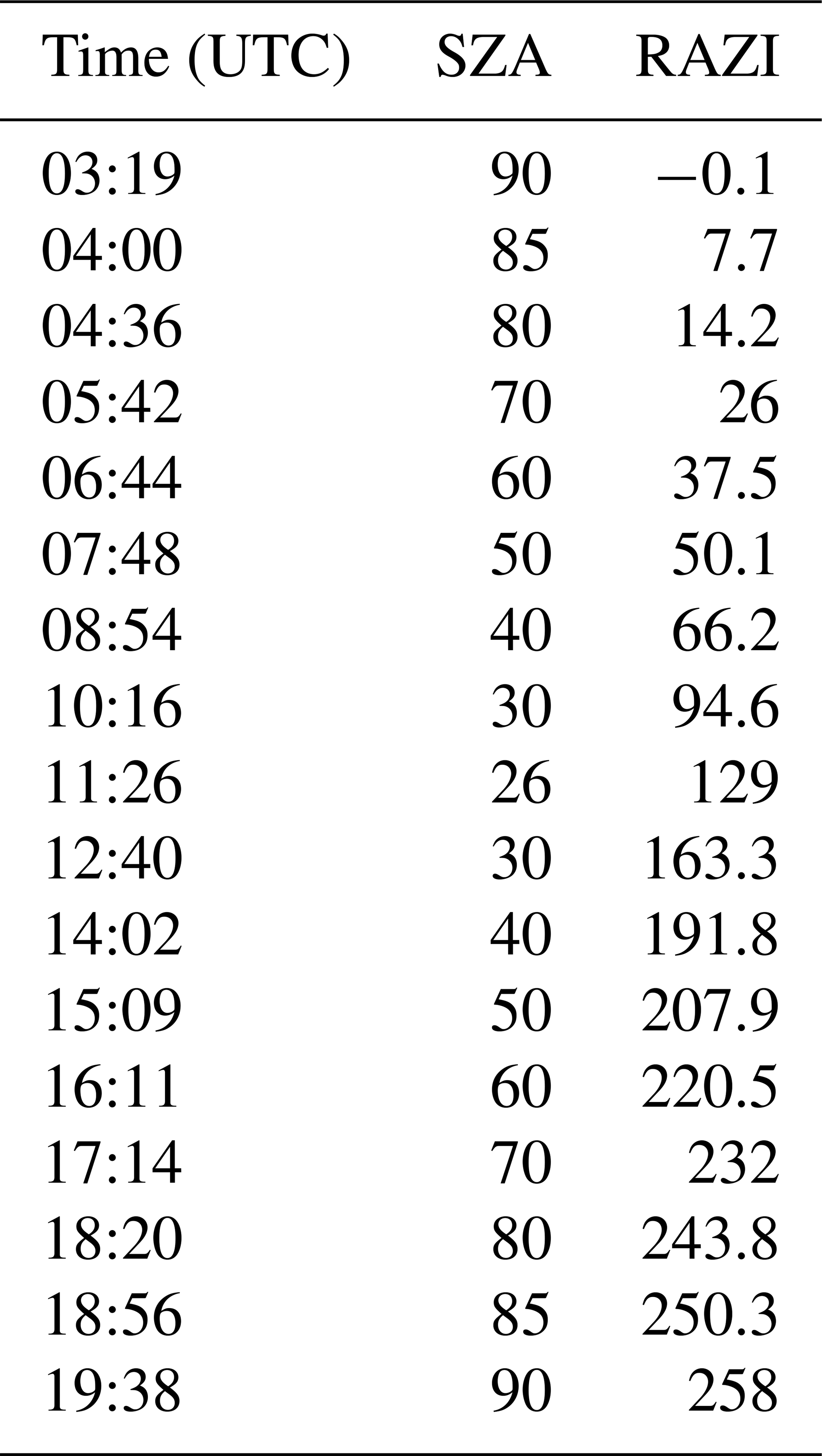
Table A3Trace gas profiles and cross sections used for the simulation of the synthetic spectra.
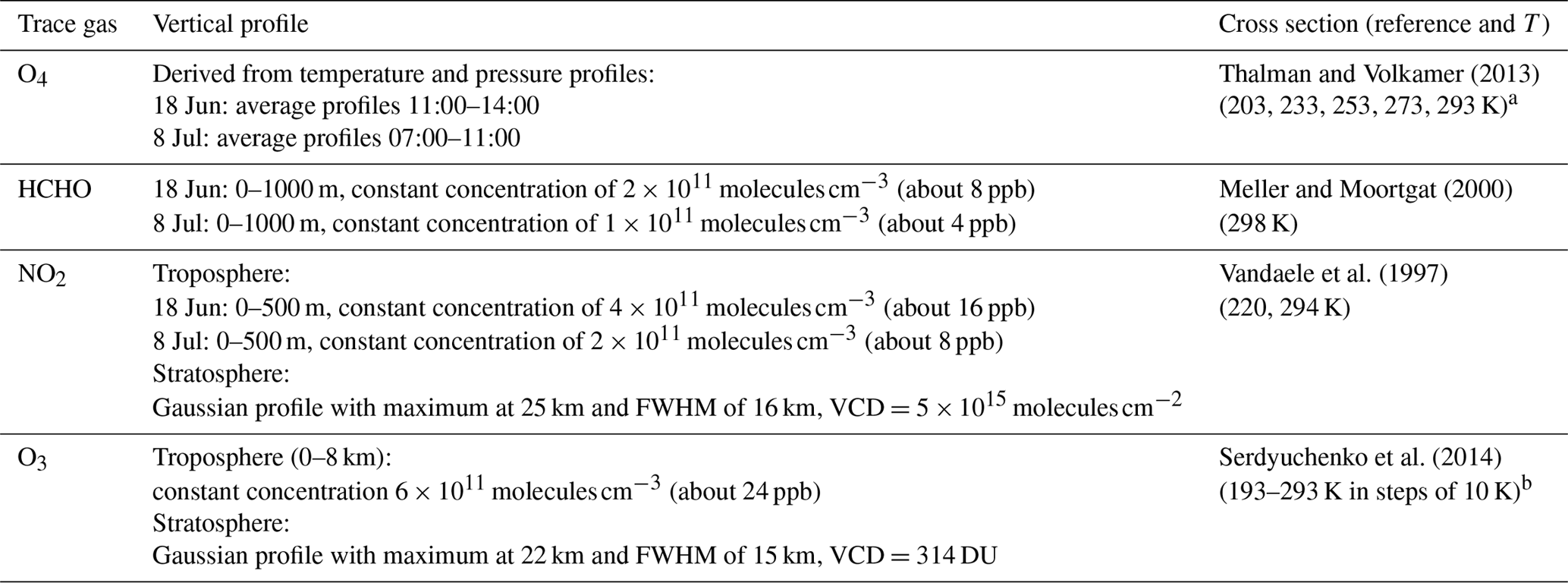
a The temperature dependence is either considered or a constant temperature
of 293 K is assumed (see text for details).
b The temperature dependence was parameterised according to Paur and Bass
(1984).
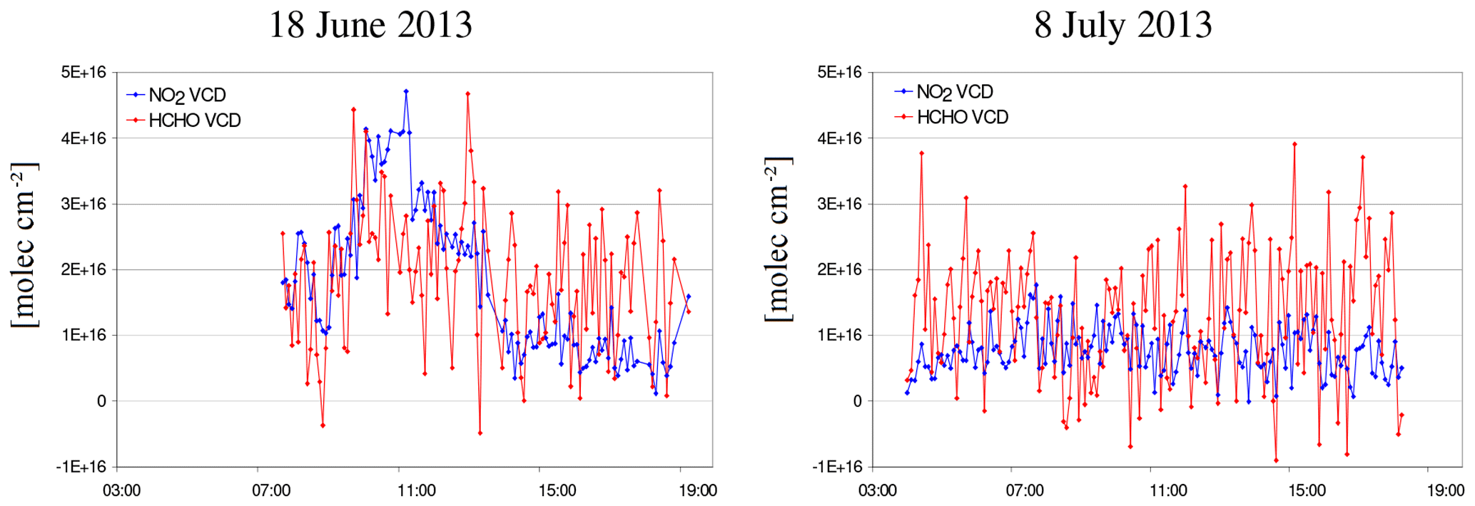
Figure A1Tropospheric VCDs of NO2 (blue) and HCHO (red) derived from measurements at 30∘ elevation using the geometric approximation.
A2 Comparison of measured and simulated O4 (d)AMFs for all azimuth and elevation angles of the MPIC MAX-DOAS measurements
The settings for the simulation of the synthetic spectra are given in Table 6 and Tables A1, A2 and A3 in Appendix A1. Measurements are analysed using the standard settings (see Table 7).

Figure A2Azimuth viewing directions of the four telescopes (T1 to T4) of the MPIC MAX-DOAS instrument. The azimuth angles are defined with respect to north (© Google maps).

Figure A3(a) Comparison results for 1∘ elevation angles on 8 July 2013. The upper lines indicate the O4 AMFs; the lower lines indicate the O4 dAMFs (see also Figs. 2 and 3). (b) Comparison results for 3∘ elevation angles on 8 July 2013. (c) Comparison results for 6∘ elevation angles on 8 July 2013. (d) Comparison results for 10∘ elevation angles on 8 July 2013. (e) Comparison results for 15∘ elevation angles on 8 July 2013. (f) Comparison results for 30∘ elevation angles on 8 July 2013. (g) Comparison results (only O4 AMFs) for 90∘ elevation angles on 8 July 2013.
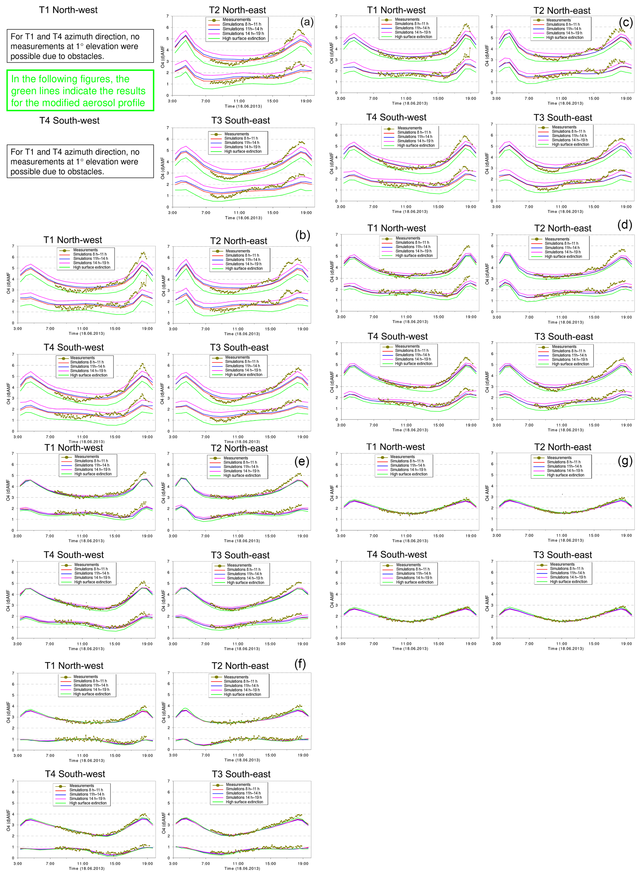
Figure A4(a) Comparison results for 1∘ elevation angles on 18 June 2013 including the RTM results for the modified aerosol extinction profile (green line). (b) Comparison results for 3∘ elevation angles on 18 June 2013. (c) Comparison results for 6∘ elevation angles on 18 June 2013. (d) Comparison results for 10∘ elevation angles on 18 June 2013. (e) Comparison results for 15∘ elevation angles on 18 June 2013. (f) Comparison results for 30∘ elevation angles on 18 June 2013. (g) Comparison results (only O4 AMFs) for 90∘ elevation angles on 18 June 2013.
A3 Comparison of the different procedures to extract height profiles of temperature, pressure and O4 concentration
A3.1 Extraction of temperature and pressure profiles
For the 2 selected days during the MAD-CAT campaign two data sets of temperature and pressure are available: surface measurements close to the measurement site and vertical profiles from ECMWF ERA-Interim reanalysis data (see Table 5). Both data sets are used to derive the O4 concentration profiles for the three selected periods on both days. The general procedure is that first the temperature profiles are determined. In a second step, the pressure profiles are derived from the temperature profiles and the measured surface pressure. For the temperature profile extraction, three height layers are treated differently:
-
Below 1 km.
Between the surface (∼150 m above sea level) and 1 km, the temperature is linearly interpolated between the average of the in situ measurements of the respective period and the ECMWF data at 1 km (see next paragraph). This procedure is used to account for the diurnal variation of the temperature close to the surface. Here it is important to note that for this near-surface layer the highest accuracy is required, because (a) the maximum O4 concentration is located near the surface, and (b) the MAX-DOAS measurements are most sensitive close to the surface.
-
From 1 to 20 km.
In this altitude range, the diurnal variation of the temperature becomes very small. Thus, the average of the four ECMWF profiles of each day is used (for simplicity, a sixth-order polynomial is fitted to the ECMWF data).
-
Above 20 km.
In this altitude range the accuracy of the temperature profile is not critical and thus the ECMWF temperature profile for 00:00 UTC of the respective day is used for simplicity.
The temperature profiles for 8 July 2013 extracted in this way are shown in Fig. 4 (left). Close to the surface the temperature variation during the day is about 10 K.
In the next step, the pressure profiles are determined from the surface pressure (obtained from the in situ measurements) and the extracted temperature profiles according to the ideal gas law. In principle the effect of atmospheric humidity could also be taken into account, but the effect is very small for near-surface layers and is thus ignored here. The derived pressure profiles for 8 July 2013 are shown in Fig. 4 (right). Excellent agreement with the corresponding ECMWF pressure profiles is found.
Here it should be noted that in principle the ECMWF pressure profiles could also be used. However, we chose to determine the pressure profiles from the surface pressure and the extracted temperature profiles, because this procedure can also be applied if no ECMWF data (or other information on temperature and pressure profiles) are available.
If no profile data (e.g. from ECMWF) are available, temperature and pressure profiles can also be extrapolated from surface measurements, e.g. by assuming a constant lapse rate of for the altitude range between the surface and 12 km, and a constant temperature above 12 km (as stated above, uncertainties at this altitude range have only a negligible effect on the O4 VCD). If no measurements or model data are available at all, a fixed temperature and pressure profile can be used, e.g. the US standard atmosphere (United States Committee on Extension to the Standard Atmosphere, 1976).
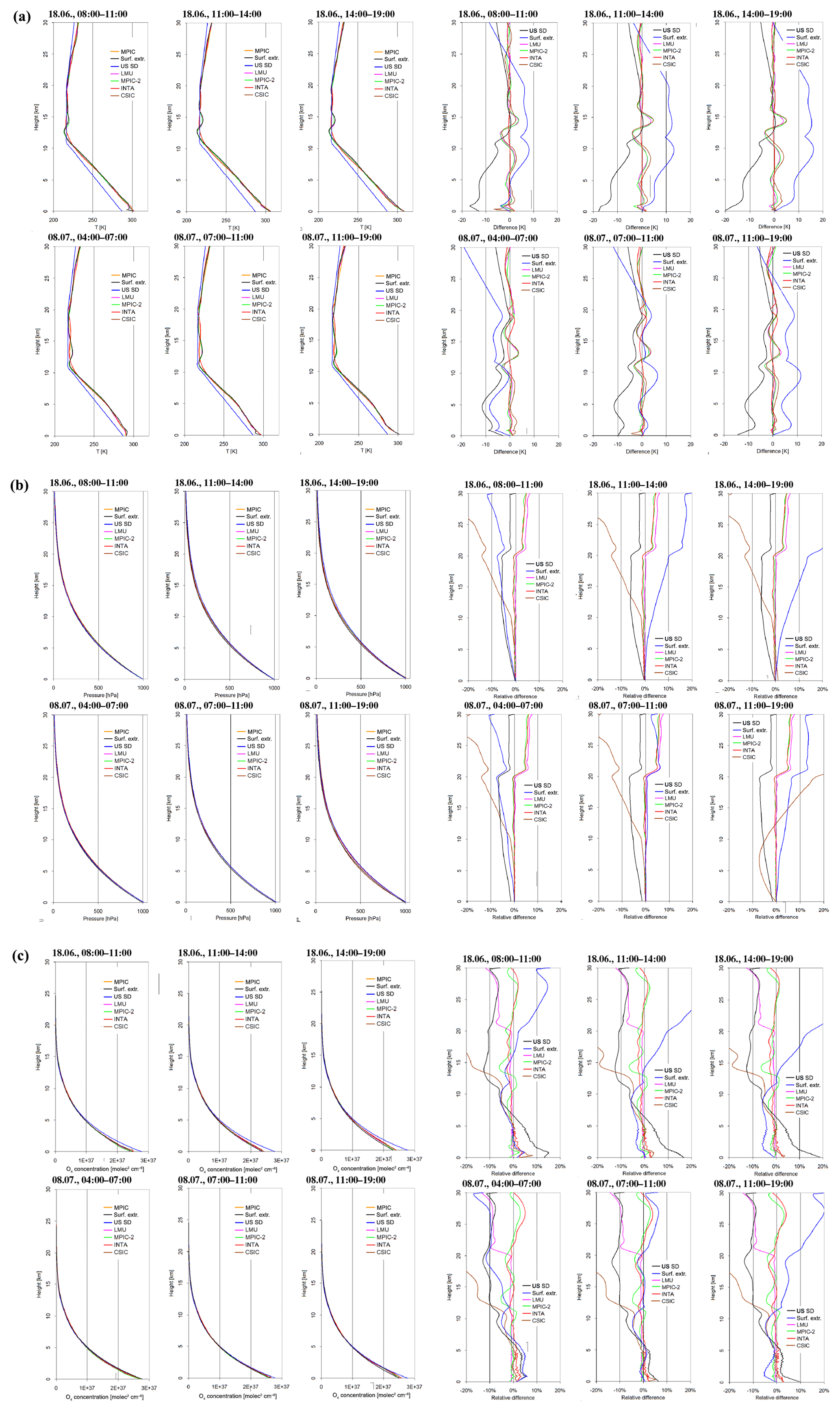
Figure A5(a) Left: Comparison of temperature profiles extracted by the different groups (also shown are the profiles from the US standard atmosphere and the profiles extrapolated from the surface measurements). Right: Differences in these profiles compared to the MPIC standard extraction. (b) Left: Comparison of pressure profiles extracted by the different groups (also shown are the profiles from the US standard atmosphere and the profiles extrapolated from the surface measurements). Right: Differences in these profiles compared to the MPIC standard extraction. (c) Left: Comparison of O4 concentration profiles extracted by the different groups (also shown are the profiles from the US standard atmosphere and the profiles extrapolated from the surface measurements). Right: Differences in these profiles compared to the MPIC standard extraction.
A3.2 Determination of the uncertainties of the O4 profiles and O4 VCDs caused by uncertainties of the input parameters
The uncertainties of the O4 profiles and O4 VCDs are derived by varying the input parameters according to their uncertainties. The following results are obtained:
-
The variation of the temperature (whole profile) by about 2 K leads to variations of the O4 concentration (or O4 VCD) by about 0.8 %.
-
The variation of the surface pressure by about 3 hPa leads to variations of the O4 concentration (or O4 VCD) by about 0.7 %.
-
The effect of uncertainties of the relative humidity depends strongly on temperature: for surface temperatures of 0, 10, 20, 30 and 35 ∘C a variation of the relative humidity of 30 % leads to variations of the O4 concentration (or O4 VCDs) of about 0.15 %, 0.3 %, 0.6 %, 1.2 % and 1.6 %, respectively. If the effect of atmospheric humidity is completely ignored (dry air is assumed), the resulting O4 concentrations (or O4 VCDs) are systematically overestimated by about 0.3 %, 0.7 %, 1.3 %, 2.5 % and 4 % for surface temperatures of 0, 10, 20, 30 and 35 ∘C, respectively (assuming a relative humidity of 70 %). In this study we used the relative humidity measured by the in situ sensors. We took these values not only for the surface layers but also for the whole troposphere. Here it should be noted that the related uncertainties of the absolute humidity decrease quickly with altitude because the absolute humidity itself decreases quickly with altitude. Since both selected days were warm or even hot summer days, we estimate the uncertainties of the O4 concentration and O4 VCDs due to uncertainties of the relative humidity to 1 % and 0.4 % on 18 June and 8 July, respectively.
Assuming that the uncertainties of the three input parameters are independent, the total uncertainty related to these parameters is estimated to be about 1.5 %.
A4 Results of the sensitivity studies of simulated and measured O4 (d)AMFs
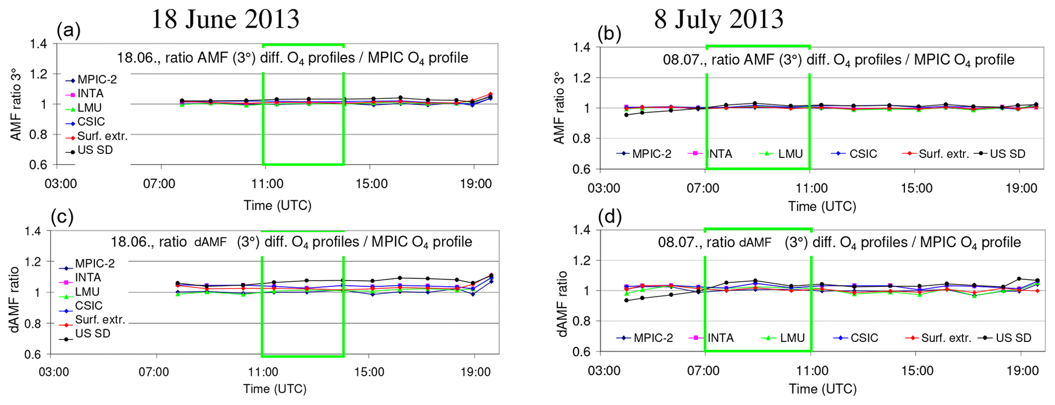
Figure A6Ratios of the O4 AMFs (a, b) and O4 dAMFs (c, d) derived for different O4 profiles vs. the standard O4 profile (MPIC) for both selected days. Besides the results for O4 profiles extracted by the different groups, the results for O4 profiles derived from the US standard atmosphere and for the extrapolation of the surface values are included.
Table A4Average ratios of O4 (d)AMFs simulated for different O4 profiles vs. the results for the standard settings (using the MPIC O4 profiles) for the middle periods on each selected day.
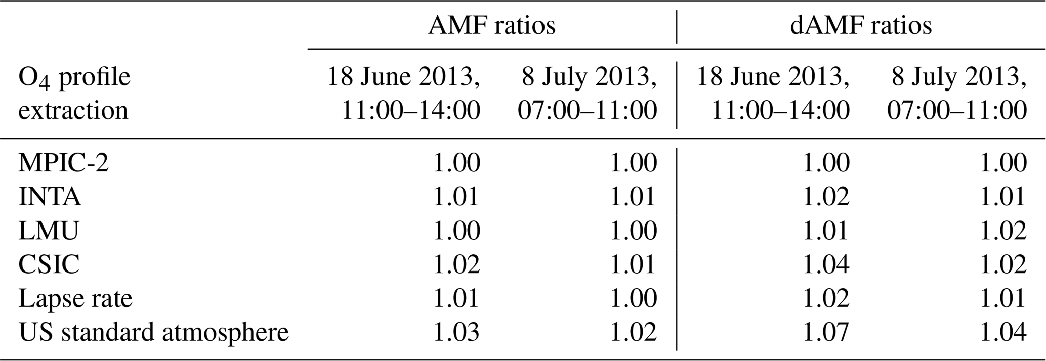
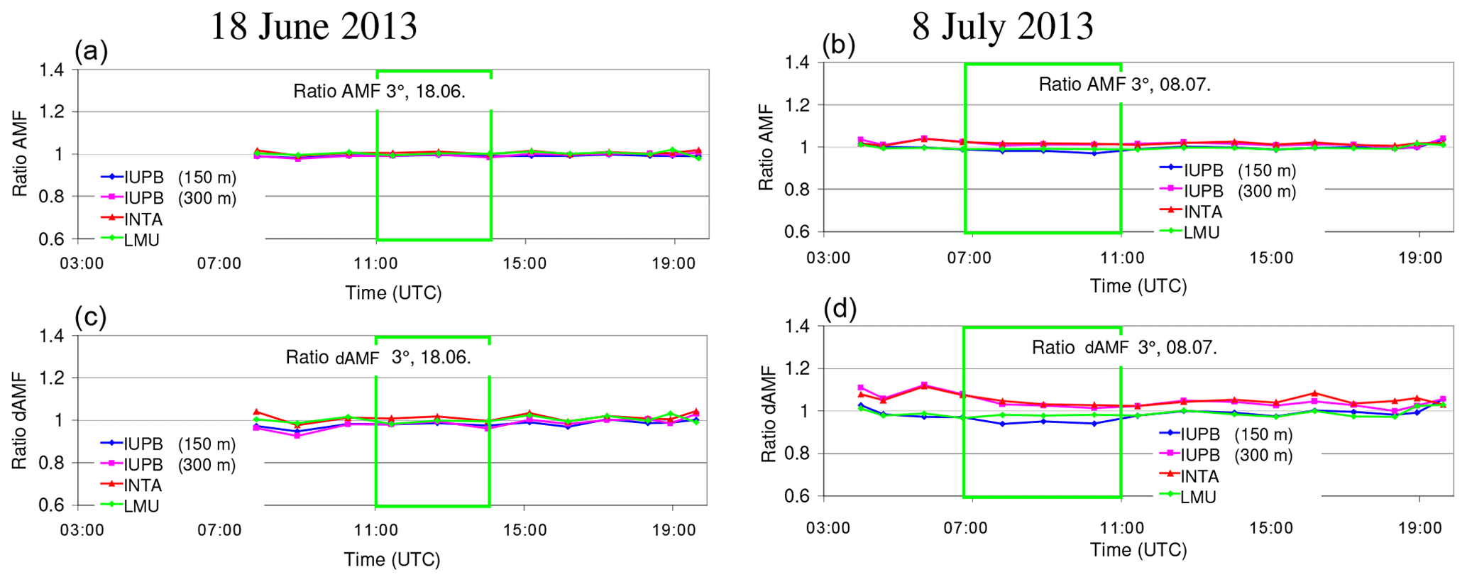
Figure A7Ratios of the O4 AMFs (a, b) and O4 dAMFs (c, d) derived for aerosol extinction profiles extracted by different groups vs. those for the standard aerosol extinction profiles (MPIC) for both selected days.
Table A5Average ratios of O4 (d)AMFs simulated for different aerosol extinction profiles vs. the results for the standard settings (using the MPIC aerosol extinction profiles) for the middle period on each selected day.


Figure A8Ratios of the O4 AMFs (a, b) and O4 dAMFs (c, d) derived for different extrapolations of the aerosol extinction profiles below 180 m vs. those for the standard settings (linearly extrapolated profiles) for both selected days.
Table A6Average ratios of O4 (d)AMFs simulated for aerosol extinction profiles with different extrapolations below 180 m vs. the results for the standard settings (linear extrapolation) for the middle period on each selected day.
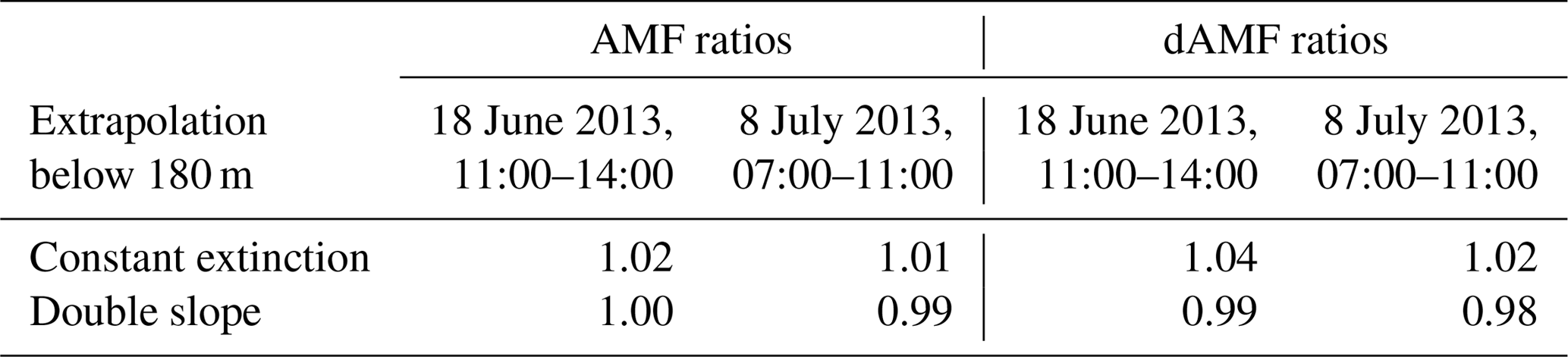
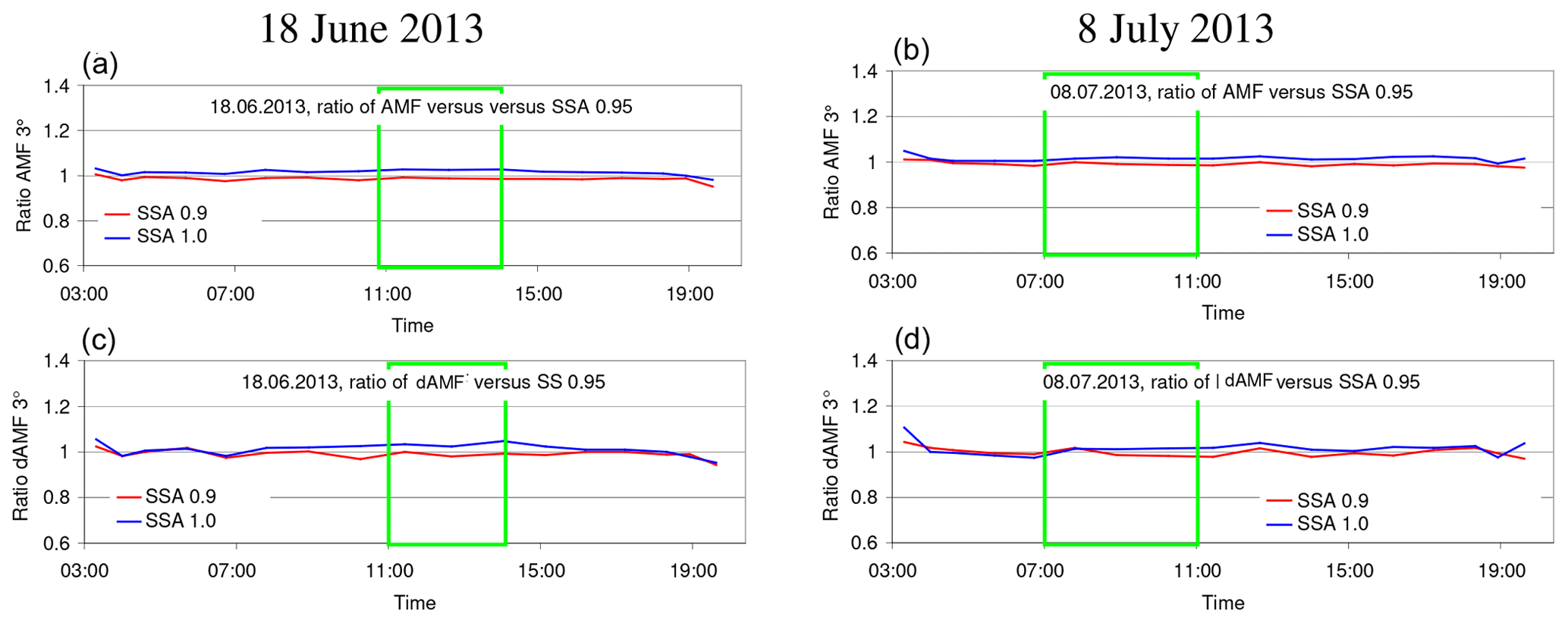
Figure A9Ratios of the O4 AMFs (a, b) and O4 dAMFs (c, d) derived for different aerosol single-scattering albedos vs. those for the standard settings (single-scattering albedo of 0.95) for both selected days.
Table A7Average ratios of O4 (d)AMFs simulated for different aerosol single-scattering albedos (SSAs) vs. the results for the standard settings (single-scattering albedo of 0.95) for the middle period on each selected day.
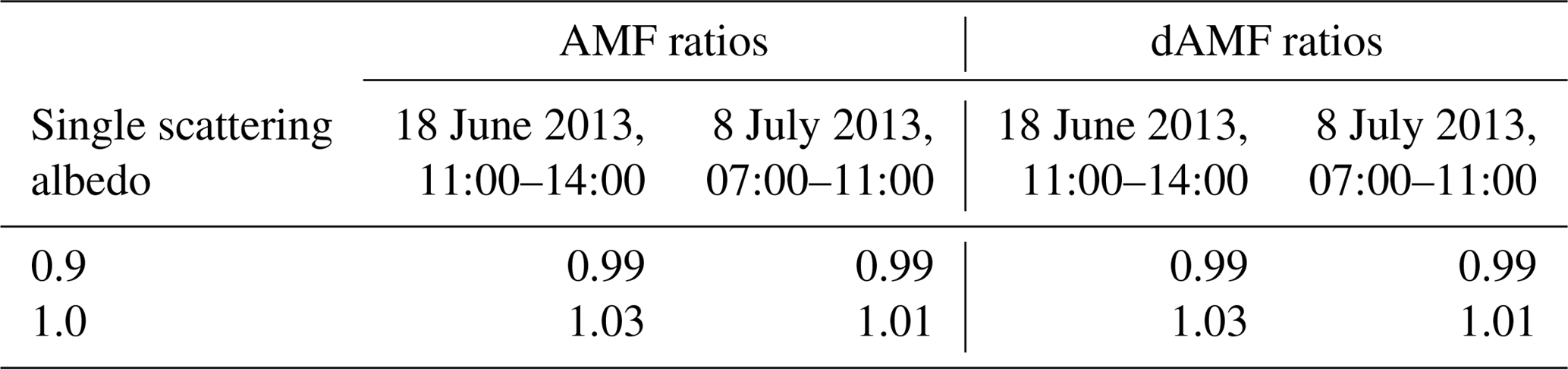
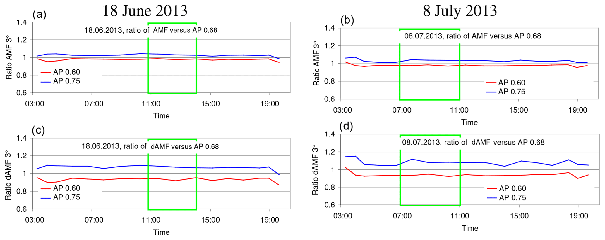
Figure A10Ratios of the O4 AMFs (a, b) and O4 dAMFs (c, d) derived for different aerosol phase functions (HG parameterisation with different asymmetry parameters) vs. those for the standard settings (asymmetry parameter of 0.68) for both selected days.
Table A8Average ratios of O4 (d)AMFs simulated for different aerosol phase functions (HG parameterisation with different asymmetry parameters (AP) vs. the results for the standard settings (asymmetry parameter of 0.68) for the middle period on each selected day.

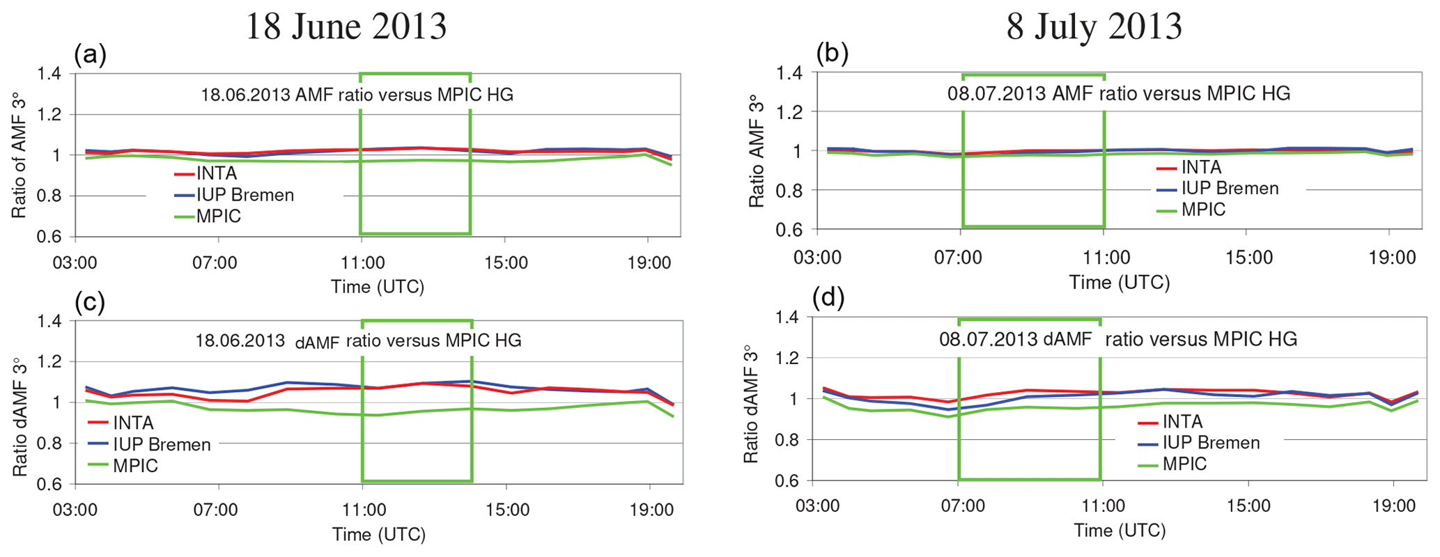
Figure A11Ratios of the O4 AMFs (a, b) and O4 dAMFs (c, d) simulated by INTA and IUP Bremen and MPIC (SCIATRAN) for phase functions derived from the sun photometer measurements vs. those simulated by MPIC using the Henyey–Greenstein phase function for an asymmetry parameter of 0.68 for both selected days.
Table A9Average ratios of O4 (d)AMFs simulated by INTA and IUP Bremen and MPIC (SCIATRAN) for phase functions derived from the sun photometer measurements vs. those simulated by MPIC using the Henyey–Greenstein phase function for an asymmetry parameter of 0.68 for the middle period on each selected day.
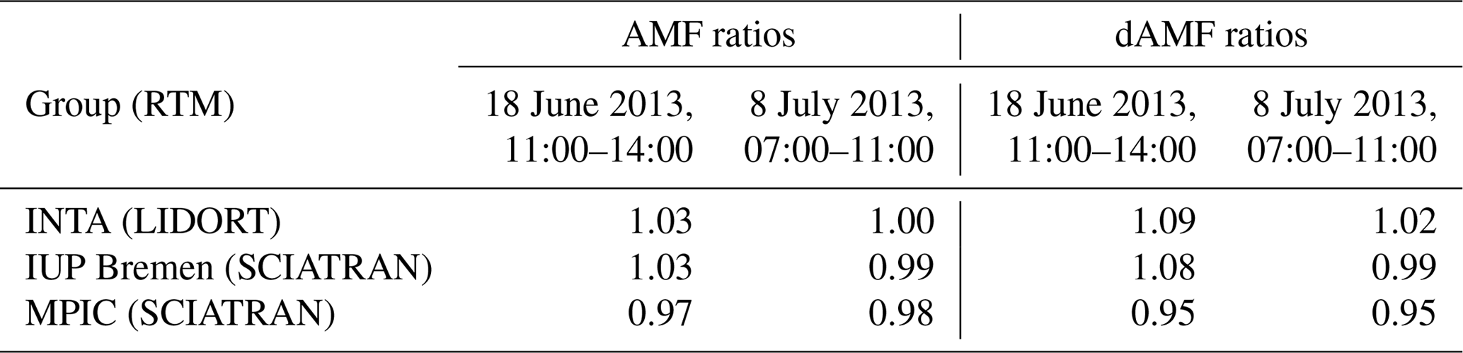
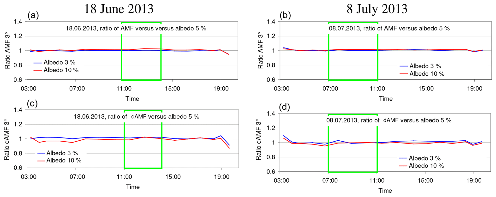
Figure A12Ratios of the O4 AMFs (a, b) and O4 dAMFs (c, d) for different surface albedos vs. those for an albedo of 5 % for both selected days.
Table A10Average ratios of O4 (d)AMFs for different surface albedos vs. those for an albedo of 5 % for the middle period on each selected days.
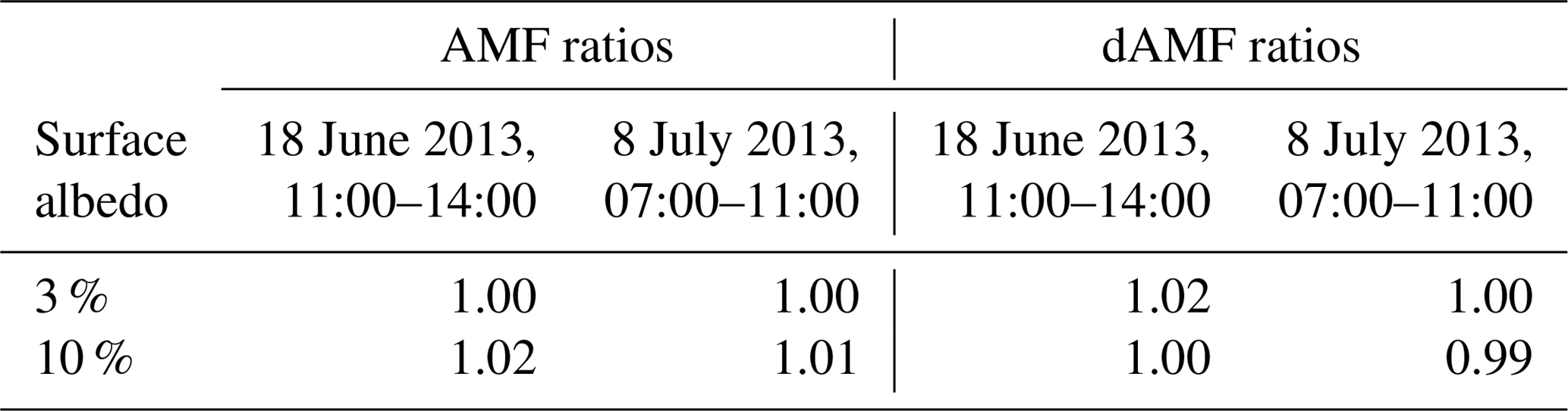
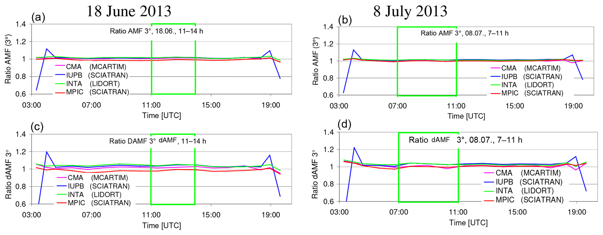
Figure A13Ratios of the O4 AMFs (a, b) and O4 dAMFs (c, d) simulated by different groups using different radiative transfer models vs. those for the MPIC simulations using McArtim for both selected days.
Table A11Average ratios of O4 (d)AMFs simulated by different groups using different radiative transfer models vs. those for the MPIC simulations using McArtim for the middle period on each selected day.
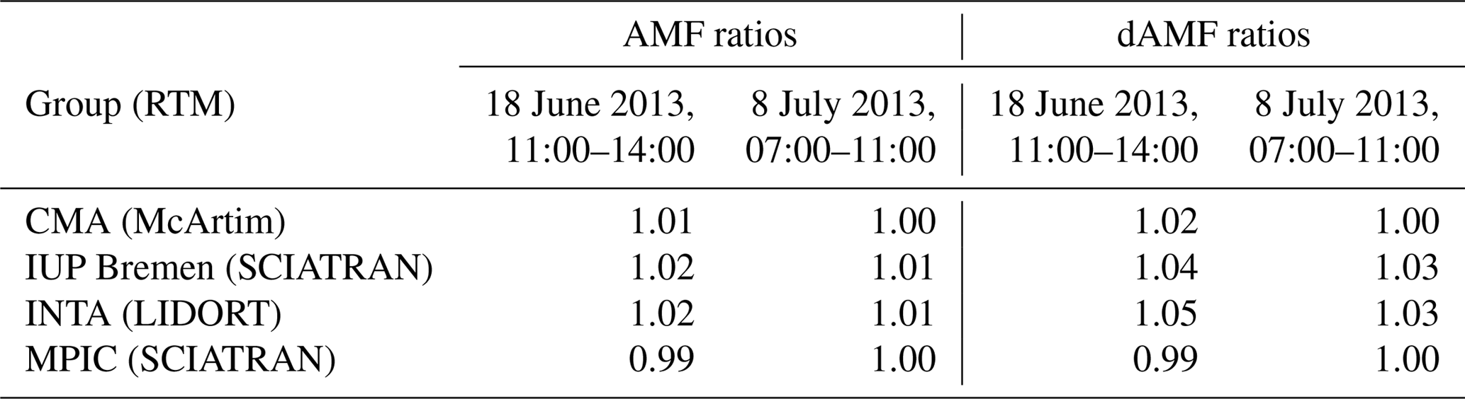
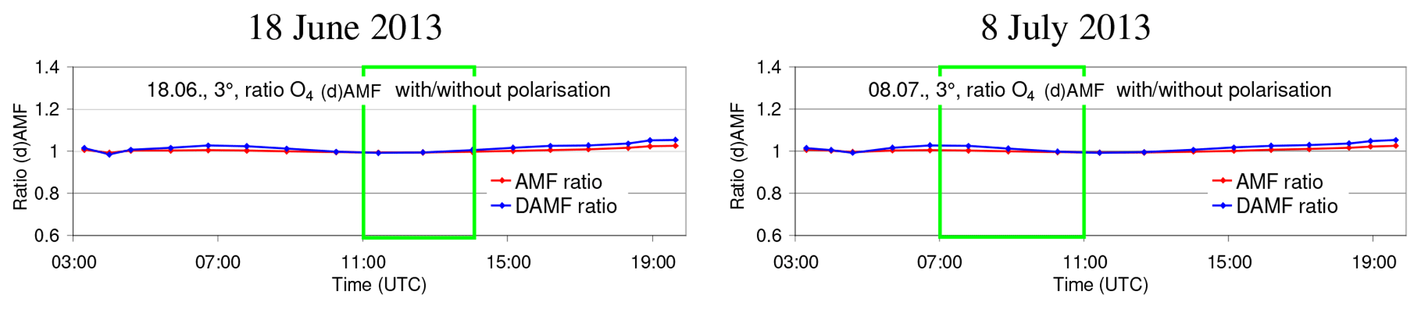
Figure A14Ratios of the O4 (d)AMFs considering polarisation vs. those without considering polarisation for both selected days.
Table A12Average ratios of O4 (d)AMFs considering polarisation vs. those without considering polarisation for the middle period on each selected day.
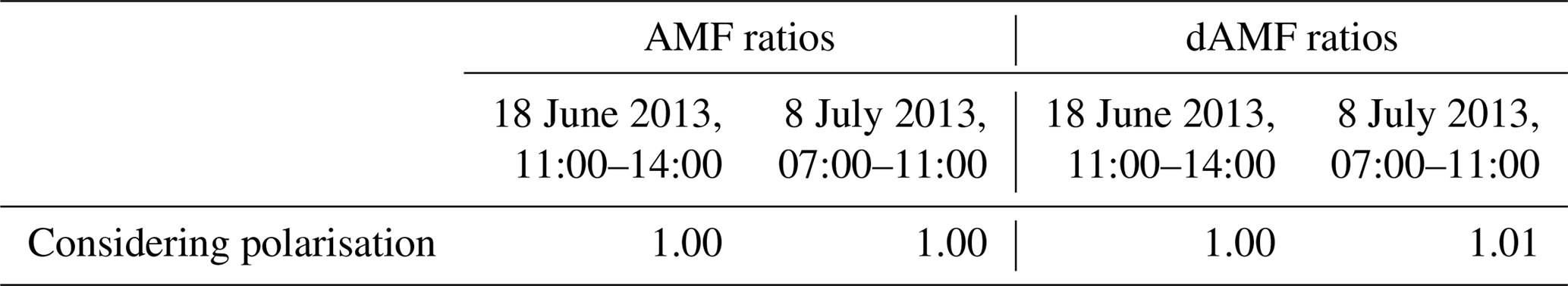
Table A13Average ratios of O4 (d)AMFs derived from synthetic spectra vs. those obtained from radiative transfer simulations at 360 nm for the middle period on each selected day.
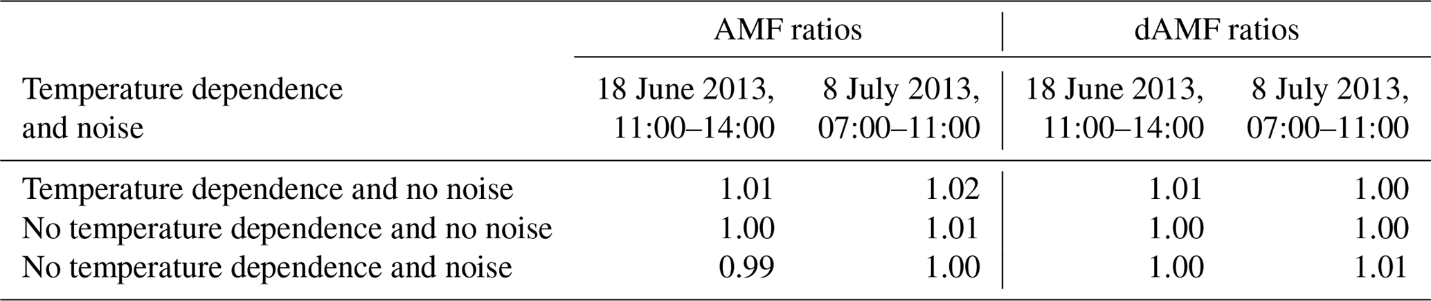
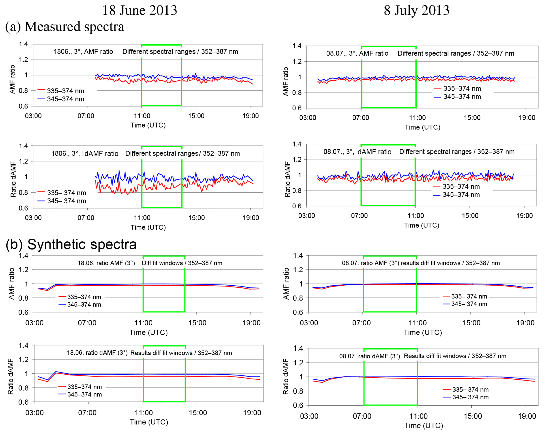
Figure A15Ratios of the O4 (d)AMFs derived for different fit windows vs. those for the standard fit window (352–387 nm) for both selected days (a: results for spectra measured by the MPIC instrument; b: results for synthetic spectra when taking into account the temperature dependence of the O4 cross section).
Table A14Average ratios of O4 (d)AMFs derived for different fit windows vs. those for the standard fit window (352–387 nm) for the middle period of each selected day (top: results for spectra measured by the MPIC instrument; bottom: results for synthetic spectra when taking into account the temperature dependence of the O4 cross section).
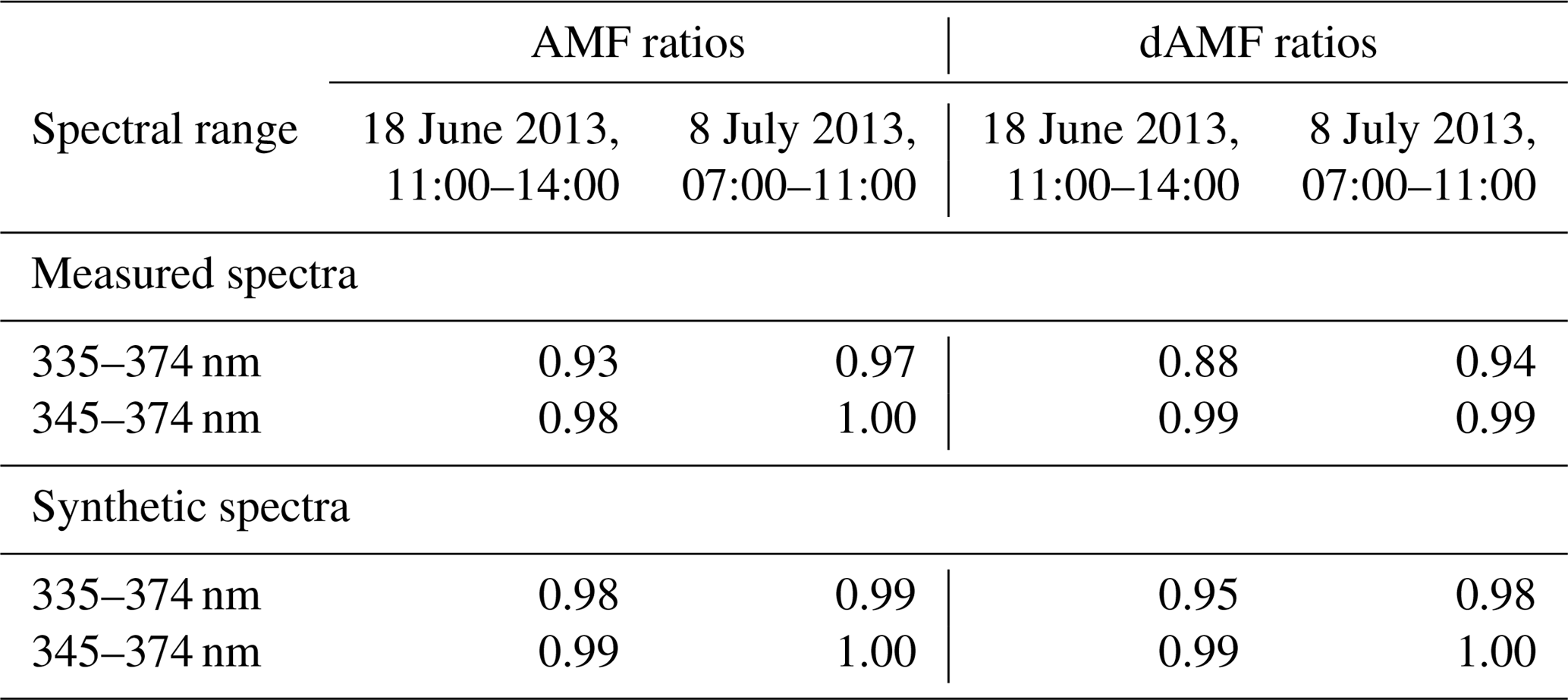
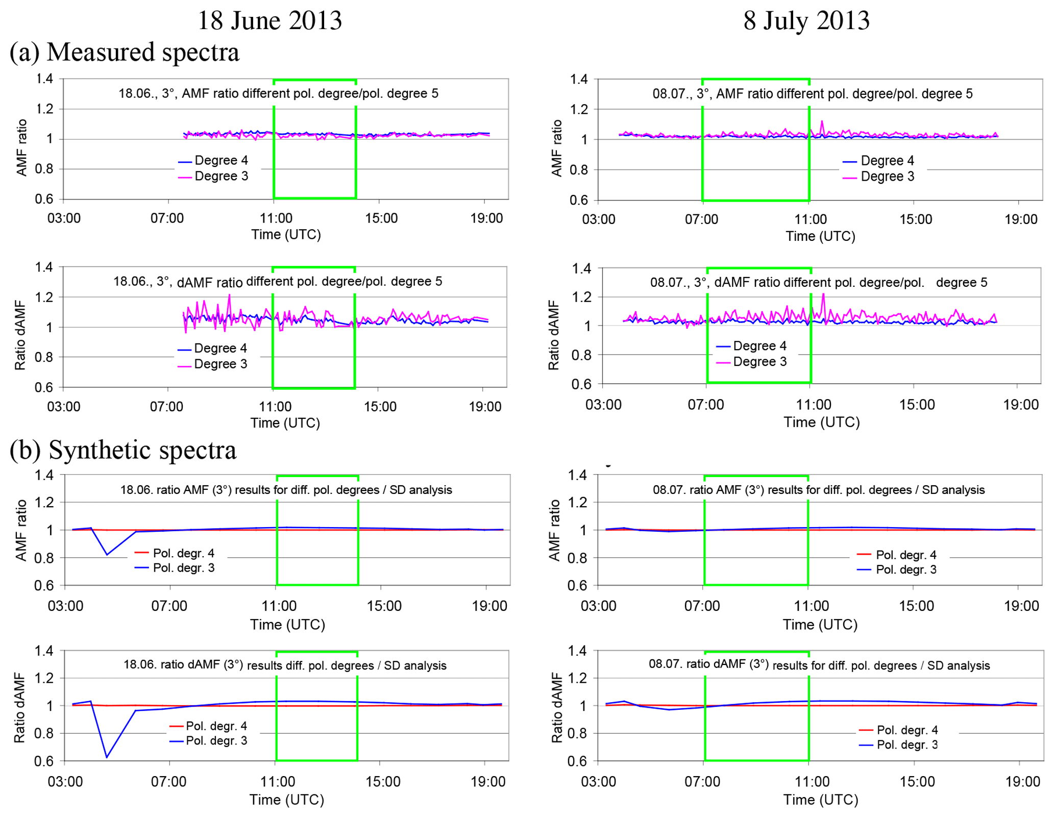
Figure A16Ratios of the O4 (d)AMFs derived for different polynomials vs. those for the standard analysis (polynomial degree 5) for both selected days (a: results for spectra measured by the MPIC instrument; b: results for synthetic spectra when taking into account the temperature dependence of the O4 cross section).
Table A15Average ratios of O4 (d)AMFs derived for different polynomials vs. those for the standard analysis (polynomial degree 5) for the middle periods on each selected day (top: results for spectra measured by the MPIC instrument; bottom: results for synthetic spectra when taking into account the temperature dependence of the O4 cross section).
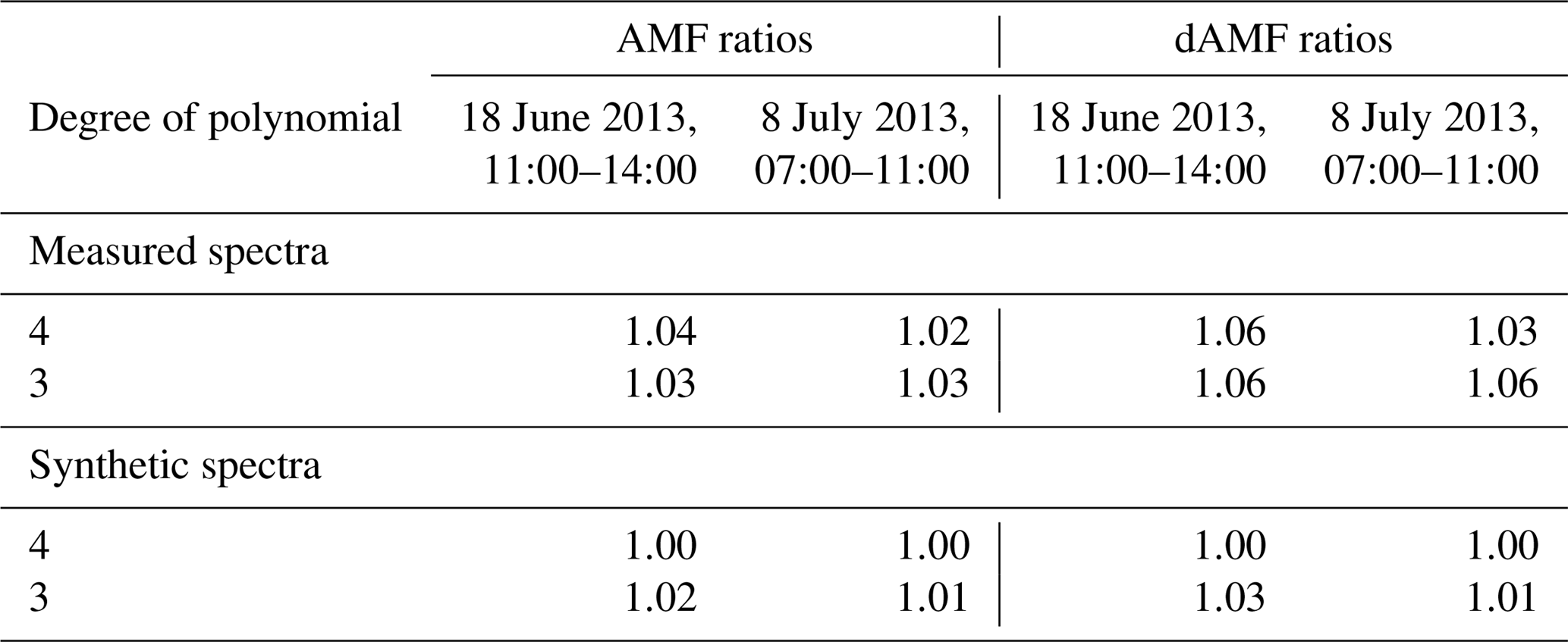
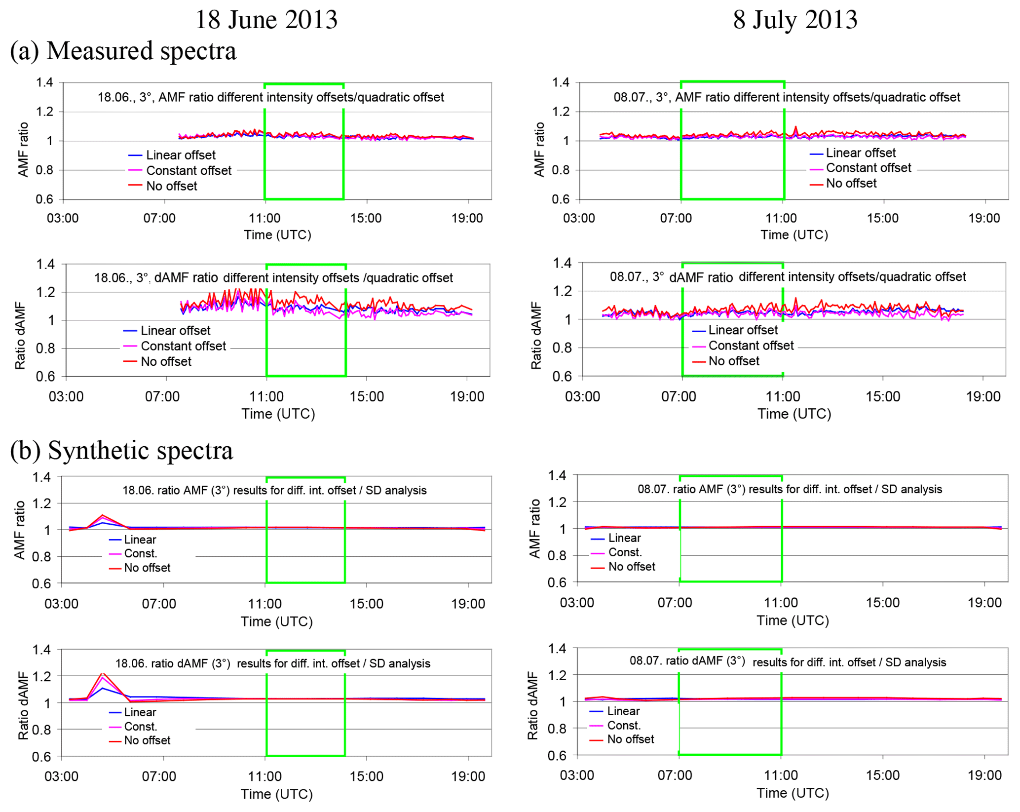
Figure A17Ratios of the O4 (d)AMFs derived for different intensity offsets vs. those for the standard analysis (intensity offset of degree 2) for both selected days (a: results for spectra measured by the MPIC instrument; b: results for synthetic spectra when taking into account the temperature dependence of the O4 cross section).
Table A16Average ratios of O4 (d)AMFs derived for different intensity offsets vs. those for the standard analysis (intensity offset of degree 2) for the middle period on each selected day (top: results for spectra measured by the MPIC instrument; bottom: results for synthetic spectra when taking into account the temperature dependence of the O4 cross section).
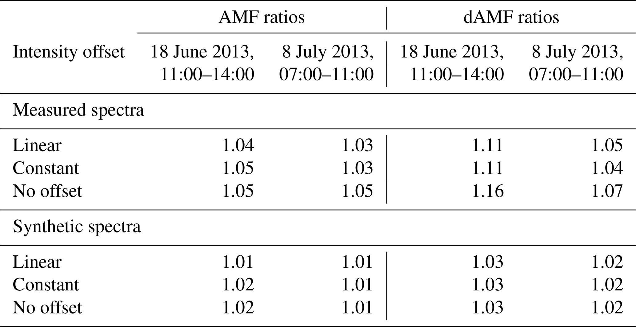
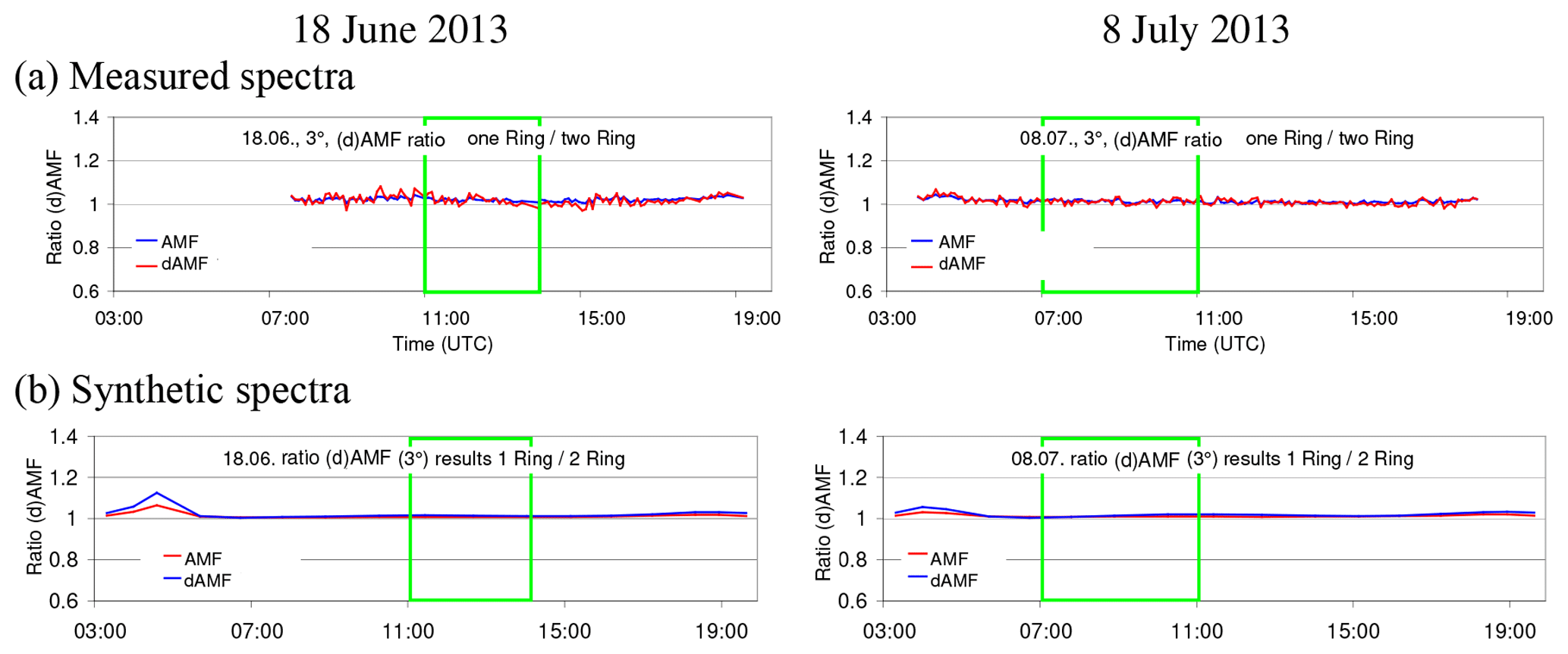
Figure A18Ratios of the O4 (d)AMFs derived for the analysis with only one Ring spectrum vs. those for the standard analysis (using two Ring spectra) for both selected days (a: results for spectra measured by the MPIC instrument; b: results for synthetic spectra when taking into account the temperature dependence of the O4 cross section).
Table A17Average ratios of O4 (d)AMFs derived for the analysis with only one Ring spectrum vs. those for the standard analysis (using two Ring spectra) for the middle period on each selected day (top: results for spectra measured by the MPIC instrument; bottom: results for synthetic spectra when taking into account the temperature dependence of the O4 cross section).
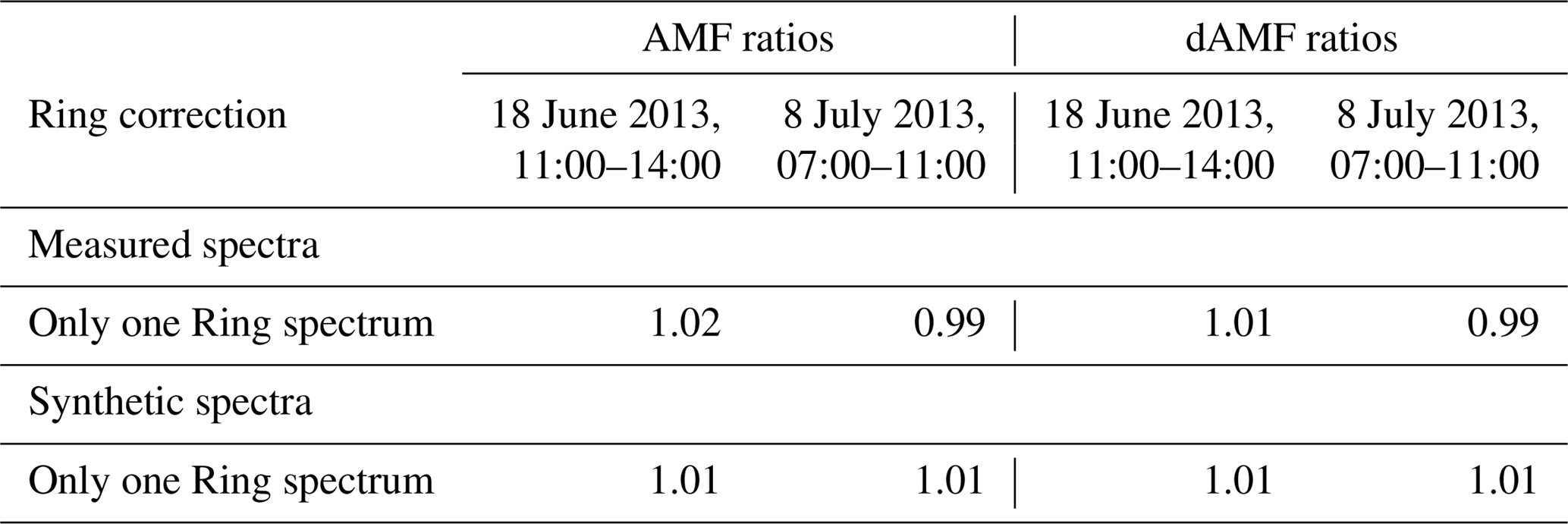
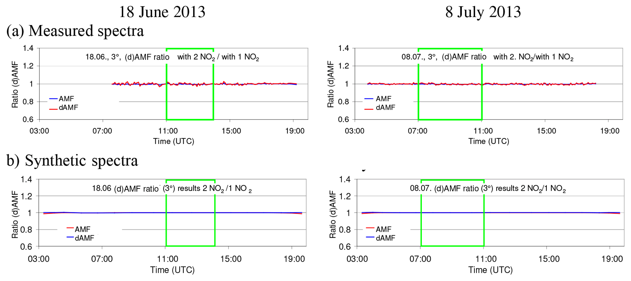
Figure A19Ratios of the O4 (d)AMFs derived for the analysis with a second NO2 cross section (for 220 K) vs. those for the standard analysis (only NO2 cross section for 294 K) for both selected days (a: results for spectra measured by the MPIC instrument; b: results for synthetic spectra when taking into account the temperature dependence of the O4 cross section).
Table A18Average ratios of O4 (d)AMFs derived for the analysis with a second NO2 cross section (for 220 K) vs. those for the standard analysis (only NO2 cross section for 294 K) for the middle period on each selected day (top: results for spectra measured by the MPIC instrument; bottom: results for synthetic spectra when taking into account the temperature dependence of the O4 cross section).
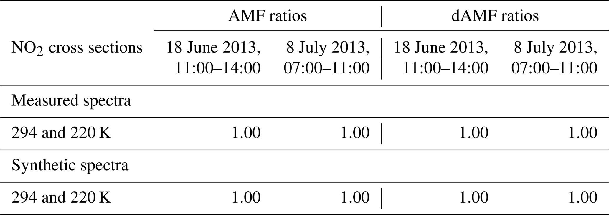
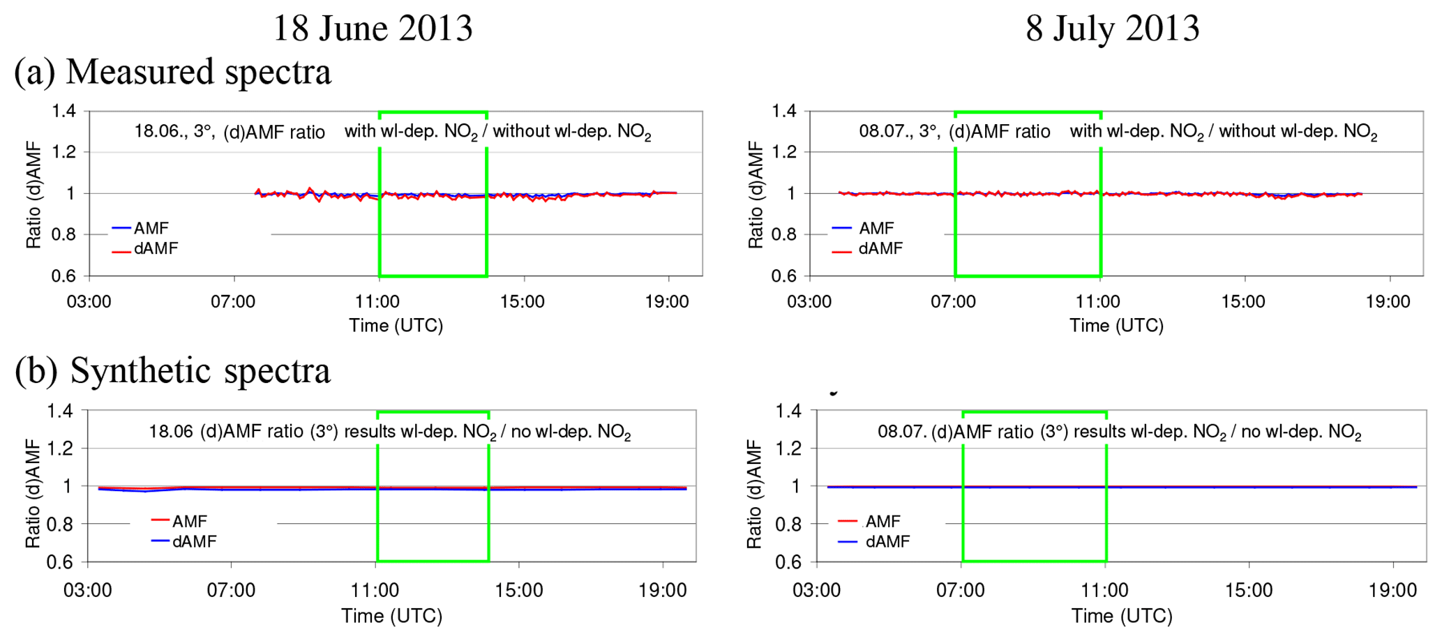
Figure A20Ratios of the O4 (d)AMFs derived for the analysis with a second NO2 cross section (cross section times wavelength) vs. those for the standard analysis (only one NO2 cross section) for both selected days (a: results for spectra measured by the MPIC instrument; b: results for synthetic spectra when taking into account the temperature dependence of the O4 cross section).
Table A19Average ratios of O4 (d)AMFs derived for the analysis with a second NO2 cross section (cross section times wavelength) vs. those for the standard analysis (only one NO2 cross section) for the middle period on each selected day (top: results for spectra measured by the MPIC instrument; bottom: results for synthetic spectra when taking into account the temperature dependence of the O4 cross section).
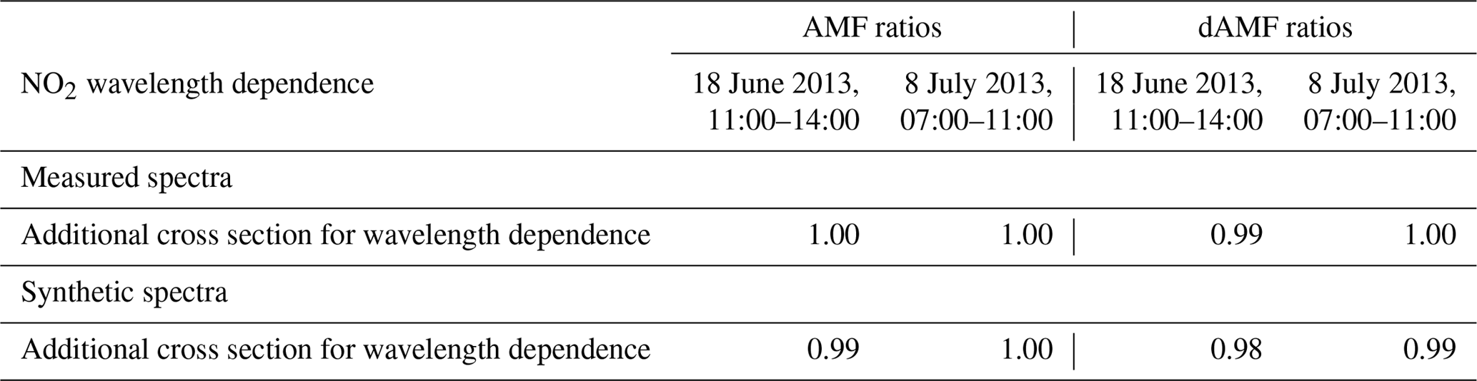
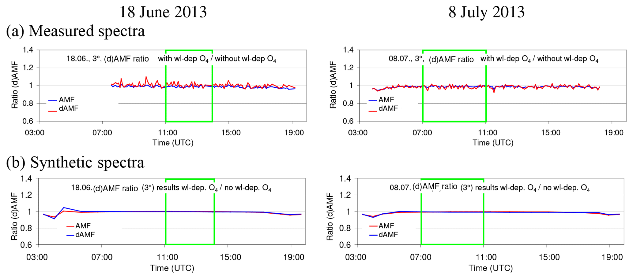
Figure A21Ratios of the O4 (d)AMFs derived for the analysis with a second O4 cross section (accounting for the wavelength dependence) vs. those for the standard analysis (only one O4 cross section) for both selected days (a: results for spectra measured by the MPIC instrument; b: results for synthetic spectra when taking into account the temperature dependence of the O4 cross section).
Table A20Average ratios of O4 (d)AMFs derived for the analysis with a second O4 cross section (accounting for the wavelength dependence) vs. those for the standard analysis (only one O4 cross section) for the middle period on each selected day (top: results for spectra measured by the MPIC instrument; bottom: results for synthetic spectra when taking into account the temperature dependence of the O4 cross section).
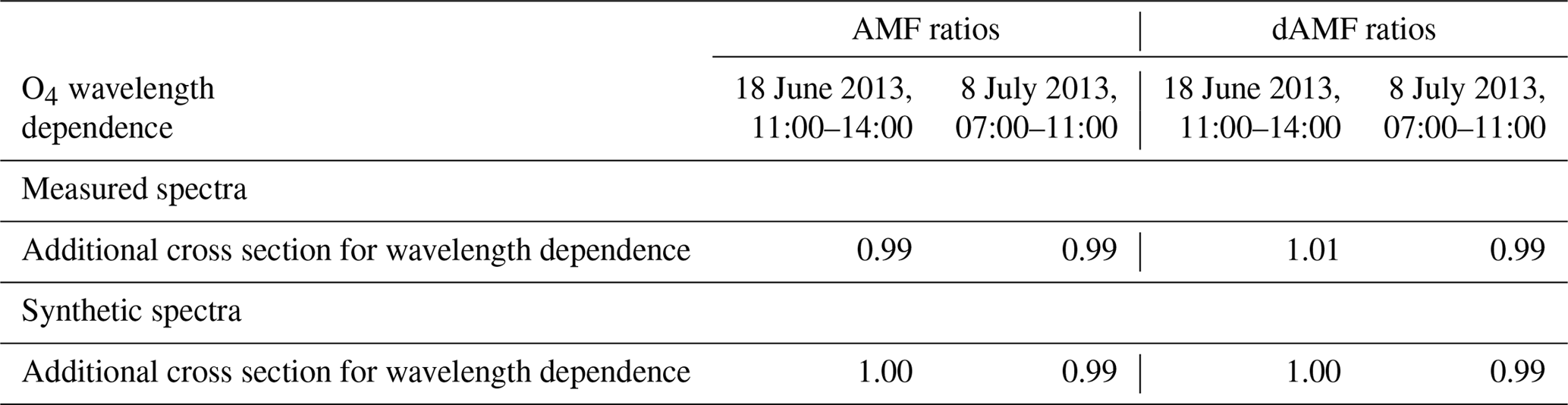
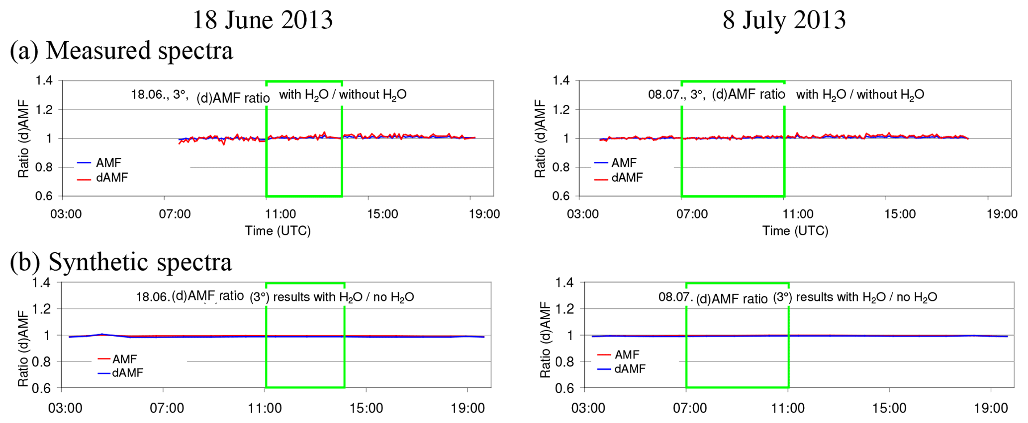
Figure A22Ratios of the O4 (d)AMFs derived for the analysis including a H2O cross section vs. those for the standard analysis (no H2O cross section) for both selected days (a: results for spectra measured by the MPIC instrument; b: results for synthetic spectra when taking into account the temperature dependence of the O4 cross section).
Table A21Average ratios of O4 (d)AMFs derived for the analysis including a H2O cross section vs. those for the standard analysis (no H2O cross section) for the standard analysis (only one O4 cross section) for the middle period on each selected day (top: results for spectra measured by the MPIC instrument; bottom: results for synthetic spectra when taking into account the temperature dependence of the O4 cross section).
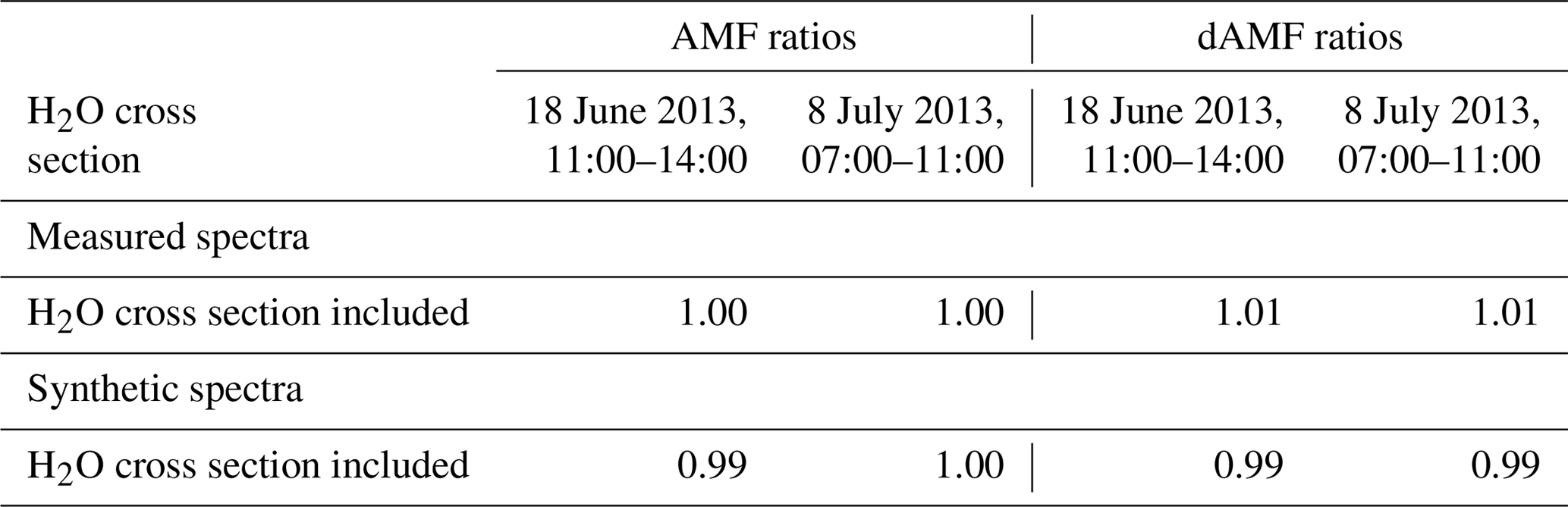
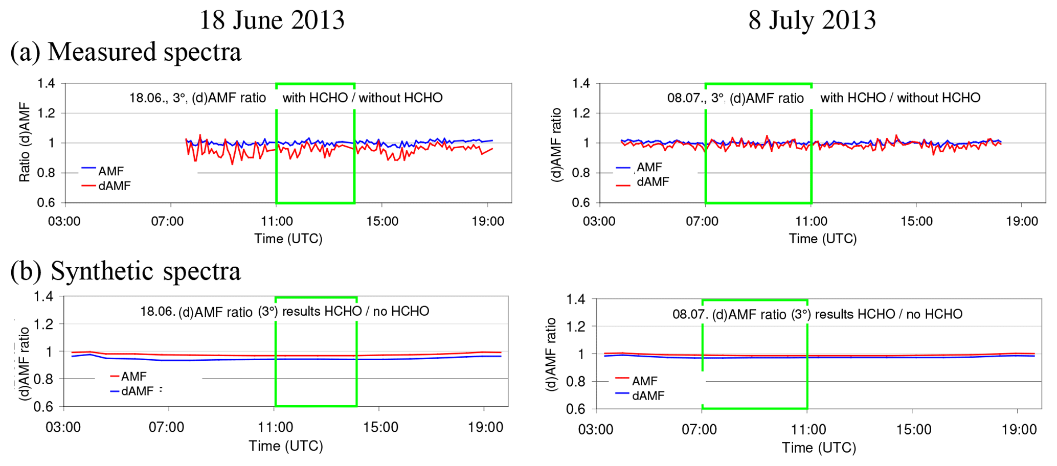
Figure A23Ratios of the O4 (d)AMFs derived for the analysis including a HCHO cross section vs. those for the standard analysis (no HCHO cross section) for both selected days (a: results for spectra measured by the MPIC instrument; b: results for synthetic spectra when taking into account the temperature dependence of the O4 cross section).
Table A22Average ratios of O4 (d)AMFs derived for the analysis including a HCHO cross section vs. those for the standard analysis (no HCHO cross section) (only one O4 cross section) for the middle period on each selected day (top: results for spectra measured by the MPIC instrument; bottom: results for synthetic spectra when taking into account the temperature dependence of the O4 cross section).
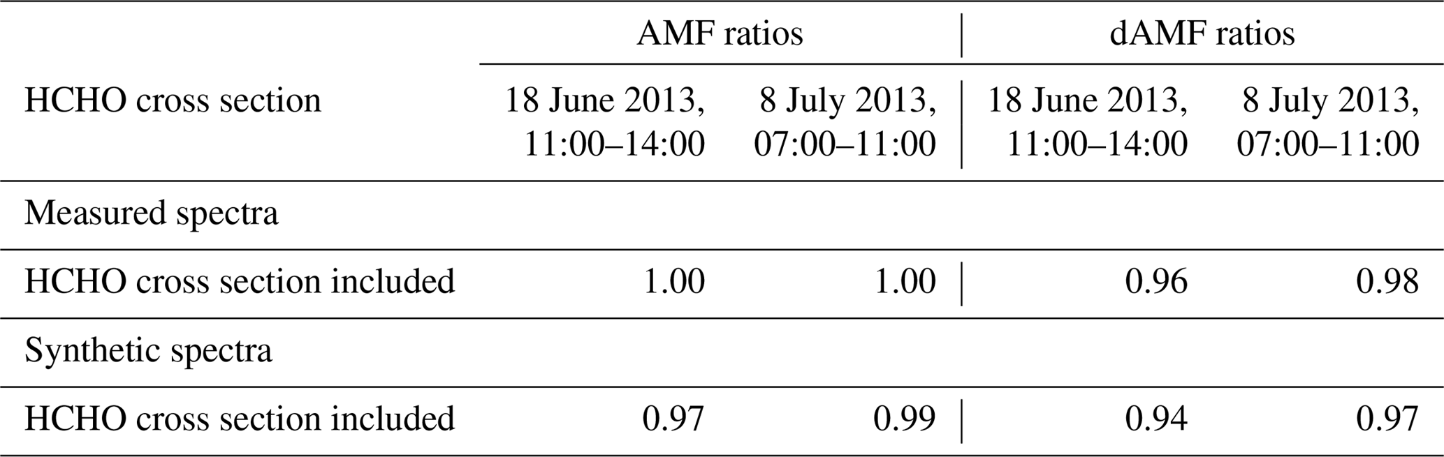
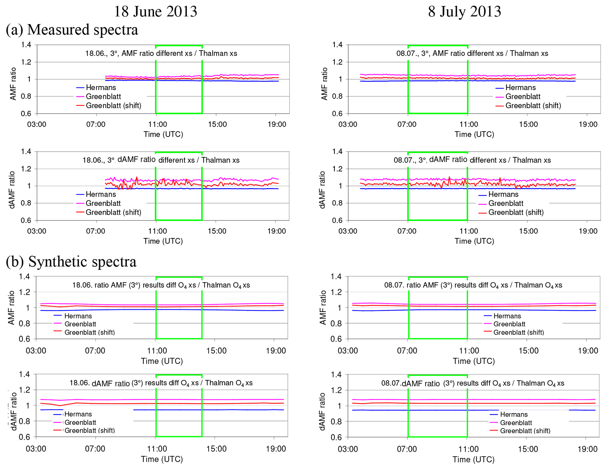
Figure A24Ratios of the O4 (d)AMFs derived for the analyses using different O4 cross sections vs. those for the standard analysis (using the Thalman and Volkamer cross section) for both selected days (a: results for spectra measured by the MPIC instrument; b: results for synthetic spectra when taking into account the temperature dependence of the O4 cross section).
Table A23Average ratios of O4 (d)AMFs derived for the analyses using different O4 cross section vs. those for the standard analysis (using the Thalman and Volkamer cross section) for the standard analysis (only one O4 cross section) for the middle period on each selected day (top: results for spectra measured by the MPIC instrument; bottom: results for synthetic spectra when taking into account the temperature dependence of the O4 cross section).
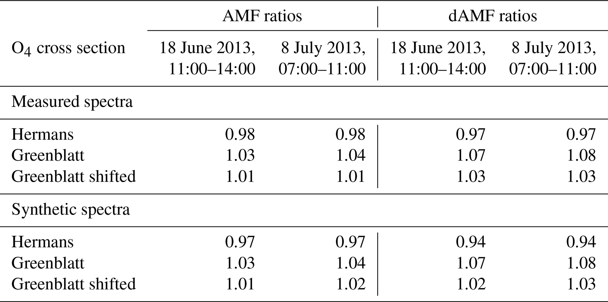
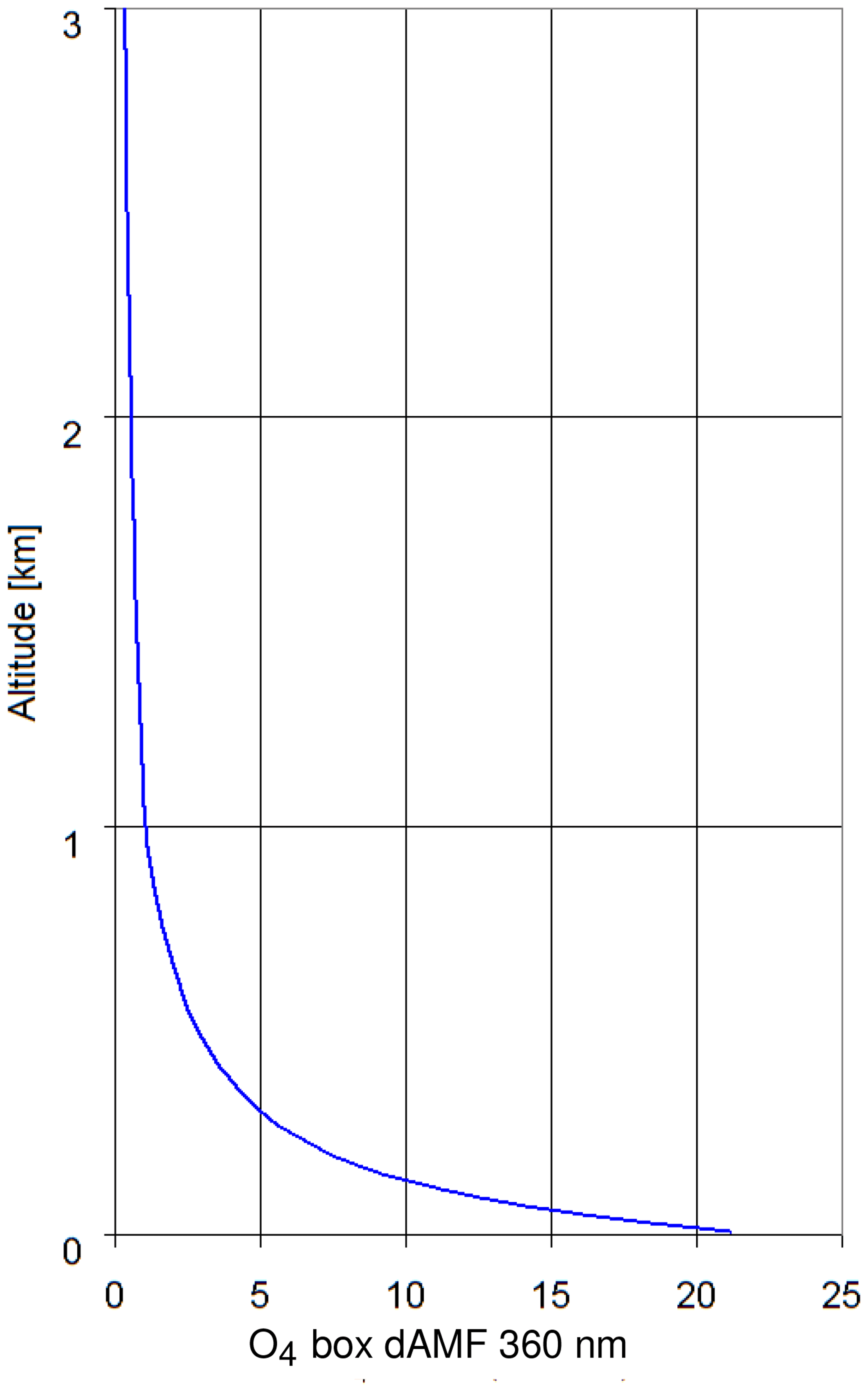
Figure A25O4 differential box AMFs (with 20 m vertical resolution) used for the simulation of the temperature-dependent O4 absorption spectra. They are averages of radiative transfer simulations for several scenarios. Simulations are performed for a surface albedo of 6 %, aerosol profiles with constant extinction between 0 and 1000 m and different AOD (0.1, 0.3, 0.7) and for all combinations of SZA (40, 60∘), RAZI (0, 90, 180∘) and elevation angles (2 and 3∘).

Figure A26Ratios of the O4 (d)AMFs derived for O4 cross sections at different temperatures (either 203 K or both 203 and 293 K) vs. those for the standard analysis (using the O4 cross section for 293 K) for both selected days (a: results for spectra measured by the MPIC instrument; b: results for synthetic spectra when taking into account the temperature dependence of the O4 cross section).
Table A24Average ratios of O4 (d)AMFs derived from O4 cross sections at different temperatures (either 203 K or both 203 and 293 K) vs. those for the standard analysis (using the O4 cross section for 293 K) for the middle period on each selected day (top: results for spectra measured by the MPIC instrument; bottom: results for synthetic spectra when taking into account the temperature dependence of the O4 cross section). For the simultaneous fit of both temperatures the results for the spectral range 345–374 nm (one O4 absorption band) are also included.
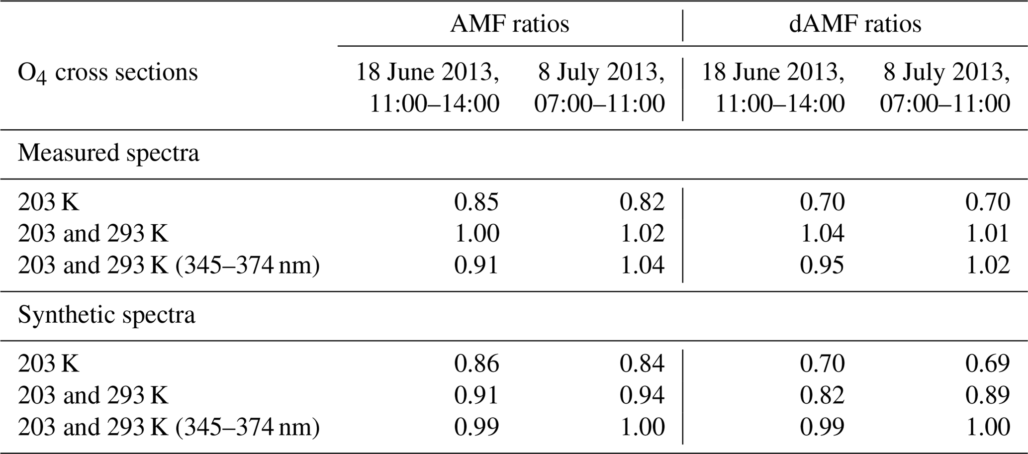
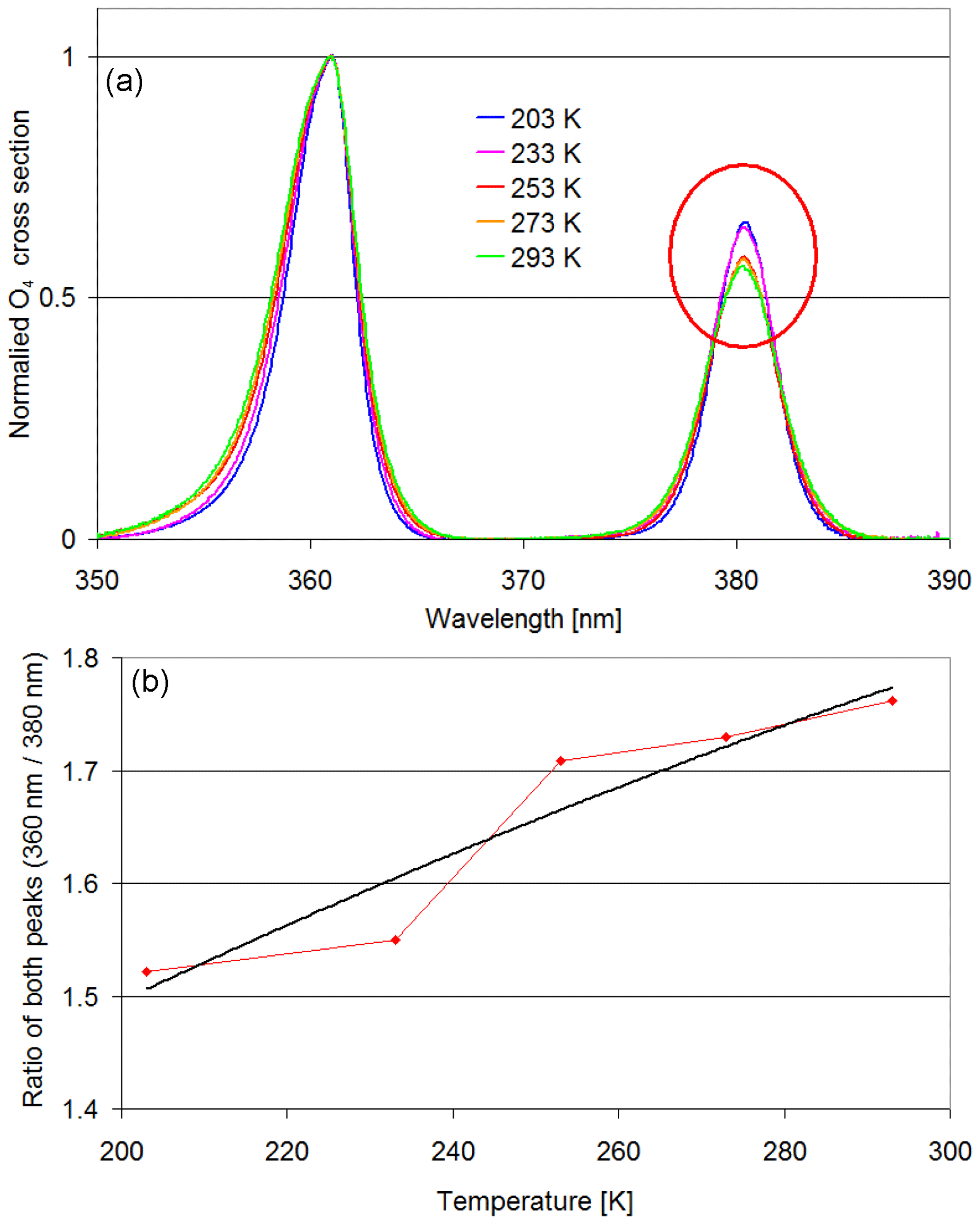
Figure A27(a) Comparison of the O4 cross sections from Thalman and Volkamer (2013) for different temperatures. The cross sections are divided by the maximum values at 360 nm. After this normalisation, the resulting values at 380 nm fall into two groups (high values for 203 and 233 K, low values for 253, 273 and 293 K). (b) Ratios of the peaks of the O4 cross section at 360 and 380 nm as a function of temperature (red points). The black curve is a fitted low-order polynomial.
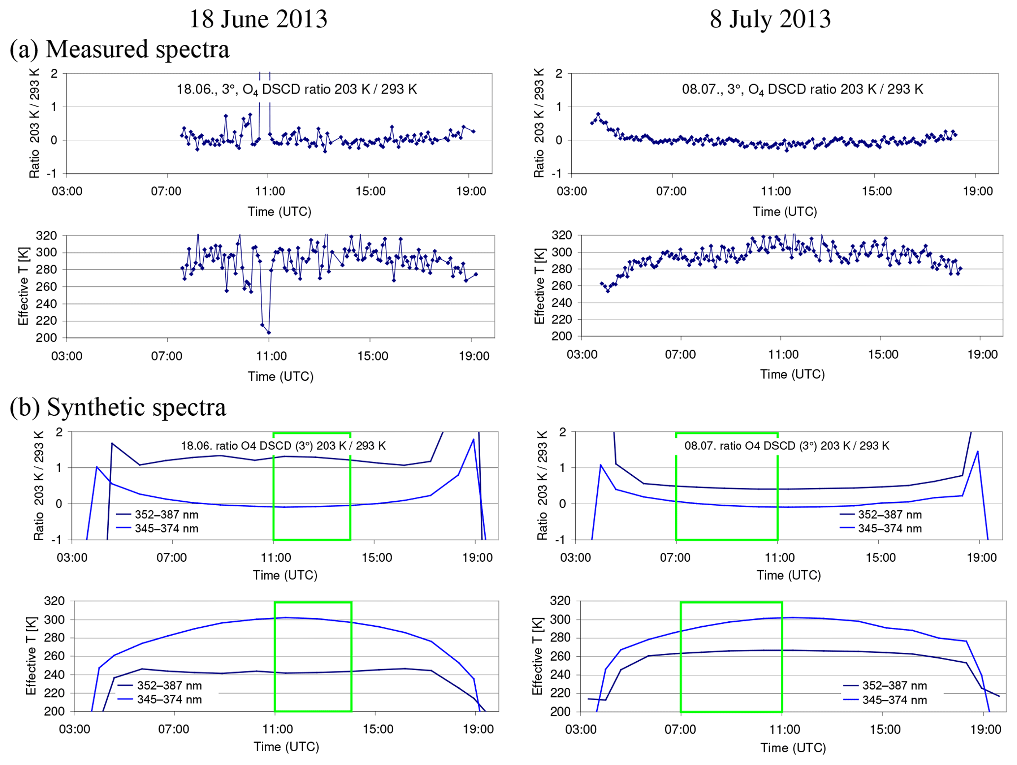
Figure A28Ratios of the retrieved O4 dSCDs for 203 and 293 K as well as the derived effective temperatures for the analyses with both cross sections included.
Table A25(a) Average ratios of O4 (d)AMFs derived from the analysis of MPIC spectra by different groups vs. the analysis of MPIC spectra by MPIC (standard analysis). (b) Average ratios of O4 (d)AMFs derived from spectra of other groups analysed by MPIC vs. the analysis of MPIC spectra by MPIC (using the same analysis settings and spectral range: 335–374 nm). (c) Average ratios of O4 (d)AMFs derived from spectra of other groups analysed by the same groups using individual analysis settings vs. the analysis of MPIC spectra by MPIC (standard analysis).
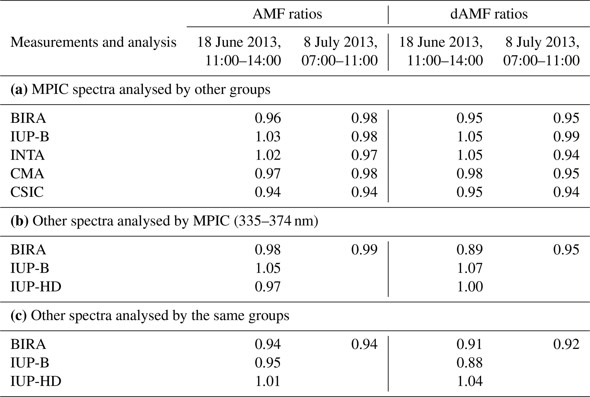
A5 Extraction of aerosol extinction profiles
In this section, the procedure for the extraction of aerosol extinction profiles is described. The aerosol profiles are derived from the ceilometer measurements (yielding the profile information) in combination with the sun photometer measurements (yielding the vertically integrated aerosol extinction, the AOD).
The raw ceilometer data consist of range-corrected backscatter profiles averaged over 15 min. The profiles range from the surface to an altitude of 15 360 m with a height resolution of 15 m. Here it is important to note that, due to limited overlap of the outgoing laser beam and the field of view of the telescope, no profile data are available below 180 m. The ceilometer profiles (hourly averages) are shown in Fig. A29 for both selected days.
The AERONET sun photometer data provide the AOD at different wavelengths (340, 360, 440, 500, 675, 870 and 1020 nm) at time intervals of 2–25 min if the direct sun is visible.
To determine profiles of aerosol extinction from the ceilometer backscatter data, several processing steps have to be performed. They are described in the subsections below. Note that in this section the individual steps are described according to the MPIC procedure. The extracted profiles from other groups differ slightly compared to the results of the MPIC procedure, especially with respect to the altitude above which the extinction was set to zero (see Fig. 9).
A5.1 Smoothing and extrapolating of the ceilometer backscatter profiles
First, the ceilometer data are averaged over several hours to reduce the scatter. For that purpose on both days three time periods are identified, for which the backscatter profile shows relatively small variations. The profiles for these periods are shown in Fig. A29. In addition to the temporal averaging, the profiles are vertically smoothed above 2 km. Above altitudes between 5 and 6 km (depending on the period) the (smoothed) ceilometer backscatter profiles become zero. Thus, the aerosol extinction profiles above these altitudes are set to zero.
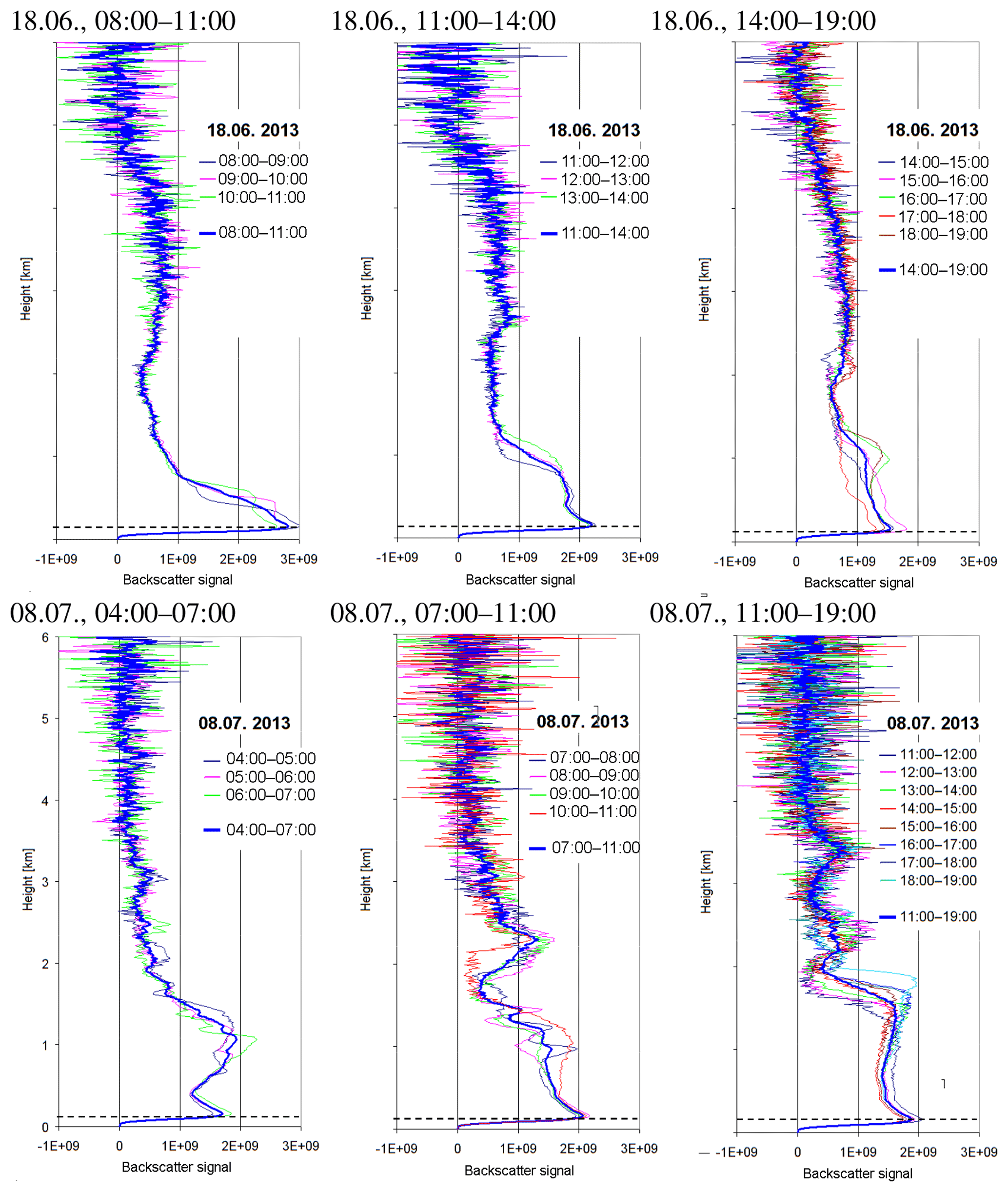
Figure A29Range-corrected backscatter profiles (hourly averages) for the three selected periods on both days. Also, the averages over the whole periods are shown (thick lines). Note that the backscatter signal below 180 m (below the dashed horizontal line) is invalid due to the limited overlap of the ceilometer instrument.
Below 180 m above the surface the ceilometer becomes “blind” for the aerosol extinction because of the insufficient overlap between the outgoing laser beam and the field of view of the telescope. Thus, the profiles have to be extrapolated down to the surface. This extrapolation constitutes an important source of uncertainty. To estimate the associated uncertainties, the extrapolation is performed in three different ways:
-
The values below 180 m are set to the value measured at 180 m.
-
The values below 180 m are linearly extrapolated assuming the same slope below 180 m as between 180 and 240 m.
-
The values below 180 m are linearly extrapolated by twice the slope between 180 and 240 m.
A5.2 Scaling of the ceilometer profiles by sun photometer AOD at 1020 nm
The scaling of the ceilometer backscatter profiles by the AOD at 1020 nm is an intermediate step, which is necessary for the correction of the aerosol self-extinction. The average AOD at 1020 nm for the different selected time periods on both days is shown in Table A26. In that table the average values at 380 nm are also shown, which are used for a second scaling (see below).
The backscatter profiles are vertically integrated and then the whole profiles are scaled by the ratio:
Here Bint indicates the integrated backscatter profile.
Note that the wavelength of the ceilometer measurements (1064 nm) is slightly different from the sun photometer measurements (1020 nm), but the difference of the AOD is negligible (typically <4 %).
Table A26Average AOD derived from the sun photometer at 1020 and 360 nm.
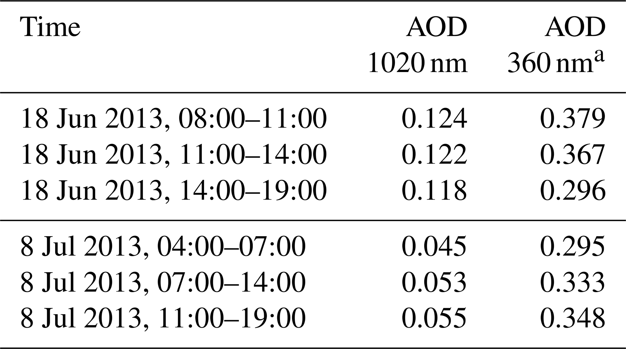
a Average of AOD at 340 and 380 nm.
A5.3 Correction of the aerosol extinction
The photons received by the ceilometer have undergone atmospheric extinction. Here, Rayleigh scattering can be ignored because of the long wavelength of the ceilometer (optical depth below 2 km is <0.001). However, while the extinction due to aerosol scattering is also small at these long wavelengths it systematically affects the ceilometer signal and has to be corrected. The extinction correction is performed according to the following formula:
Here αi represents the uncorrected extinction and αi,corr represents the corrected extinction at height layer i (with zi is the lower boundary of that height layer). Equation (A2) has to be subsequently applied to all height layers starting from the surface (z0). Note that the factor of 2 accounts for the extinction along both paths between the instrument and the scattering altitude (upward and downward). The extinction correction is performed at a vertical resolution of 15 m.
After the extinction correction, the profiles are scaled by the corresponding AOD at 360 nm (see Table A26). In Fig. A30 the profiles with and without extinction correction are shown. The extinction correction slightly increases the values at higher altitudes and decreases the values close to the surface. The effect of the extinction correction is larger on 18 June 2013 (up to 12 %).
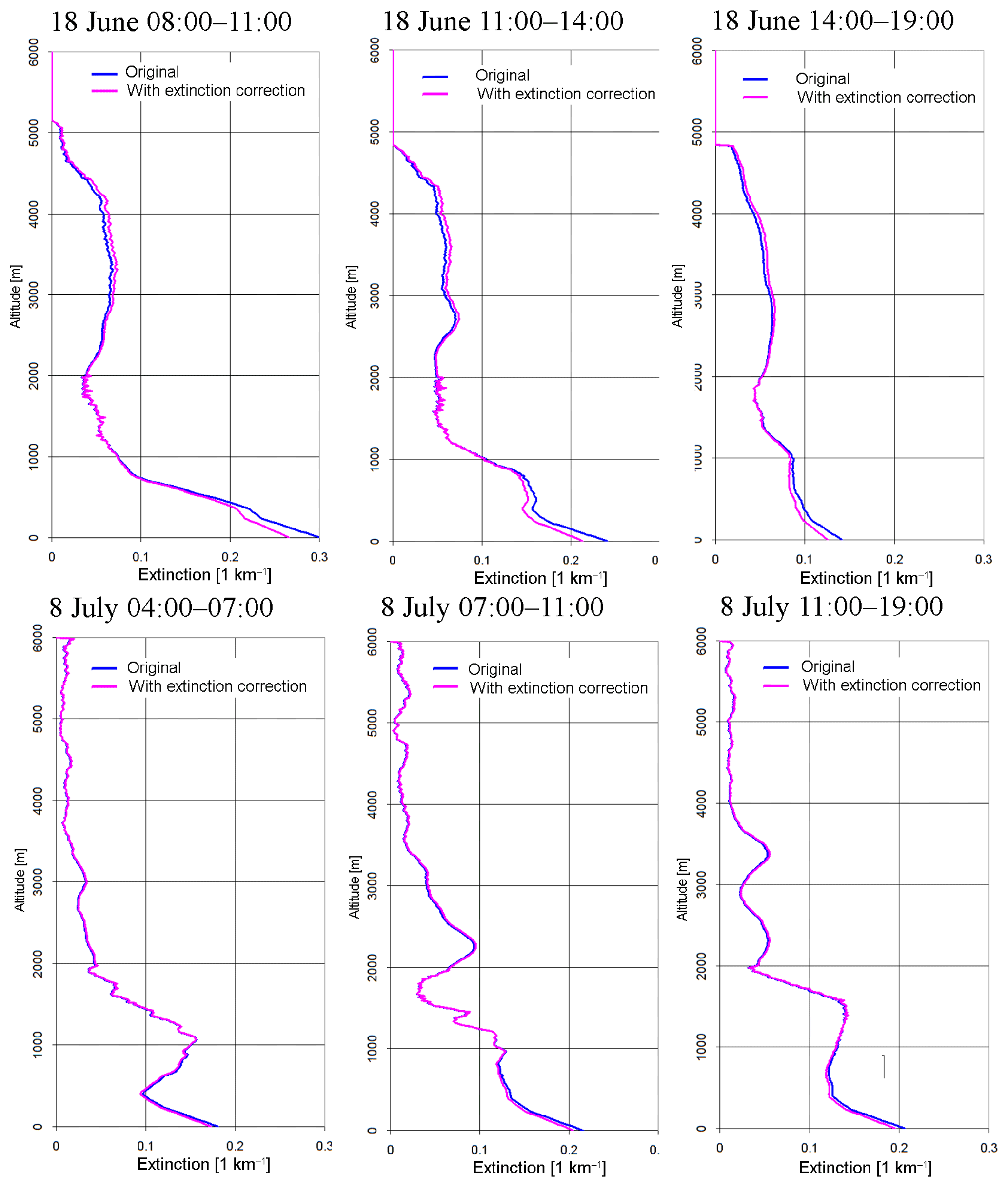
Figure A30Comparison of profiles (linear extrapolation below 180 m) without (blue) and with (magenta) extinction correction. Both profiles are scaled to the same total AOD (at 360 nm) determined from the sun photometer.
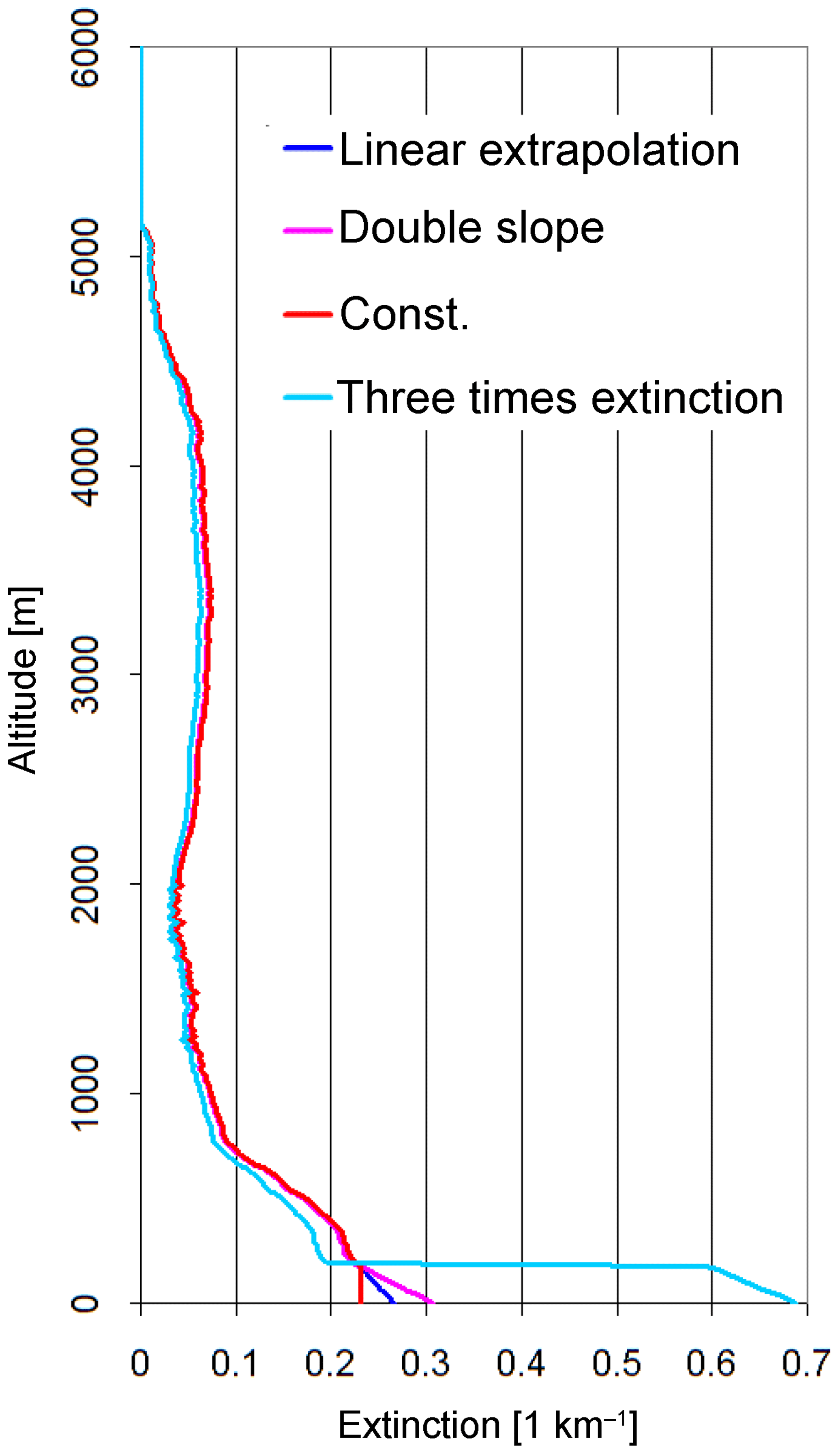
Figure A31Aerosol profile (light blue) with extreme extinction close to the surface (below 180 m, the altitude for which the ceilometer is sensitive) extracted for the first period (08:00–11:00) on 18 June 2013. Also shown are the profiles extrapolated below 180 as described above. Const. means constant below 180 m.
A5.4 Influence of a changing lidar ratio with altitude
For the extraction of the aerosol profiles described above, a fixed lidar ratio was assumed, which implies that the aerosol properties are independent from altitude. However, this is a rather strong assumption, because it can be expected that the aerosol properties (e.g. the size) change with altitude. With the available limited information, it is impossible to derive detailed information about the altitude dependence of the aerosol properties, but it can be quantified how representative the ceilometer measurements at 1064 nm are for the aerosol extinction profiles at 360 nm. For these investigations we again focus on the middle periods of both selected days. From the AERONET Almucantar observations information on the size distribution for these periods is available (see Fig. A32). On both days two pronounced modes (fine and coarse mode) are found with a much larger coarse-mode fraction on 18 June compared to 8 July (on 18 June the coarse mode is broader and shows two distinct maxima). From the AERONET observations, separate phase functions for the fine and coarse mode, as well as the relative contributions of both modes to the total AOD at 500 nm, are also available. On 18 June and 8 July the relative contributions of the coarse-mode fraction to the total AOD at 500 nm are about 39 % and 5 %, respectively (see Table A27). Assuming that the AOD of the coarse-mode fraction is independent of wavelength, the relative contributions of the coarse mode at 360 and 1064 nm can be derived (see Table A27).
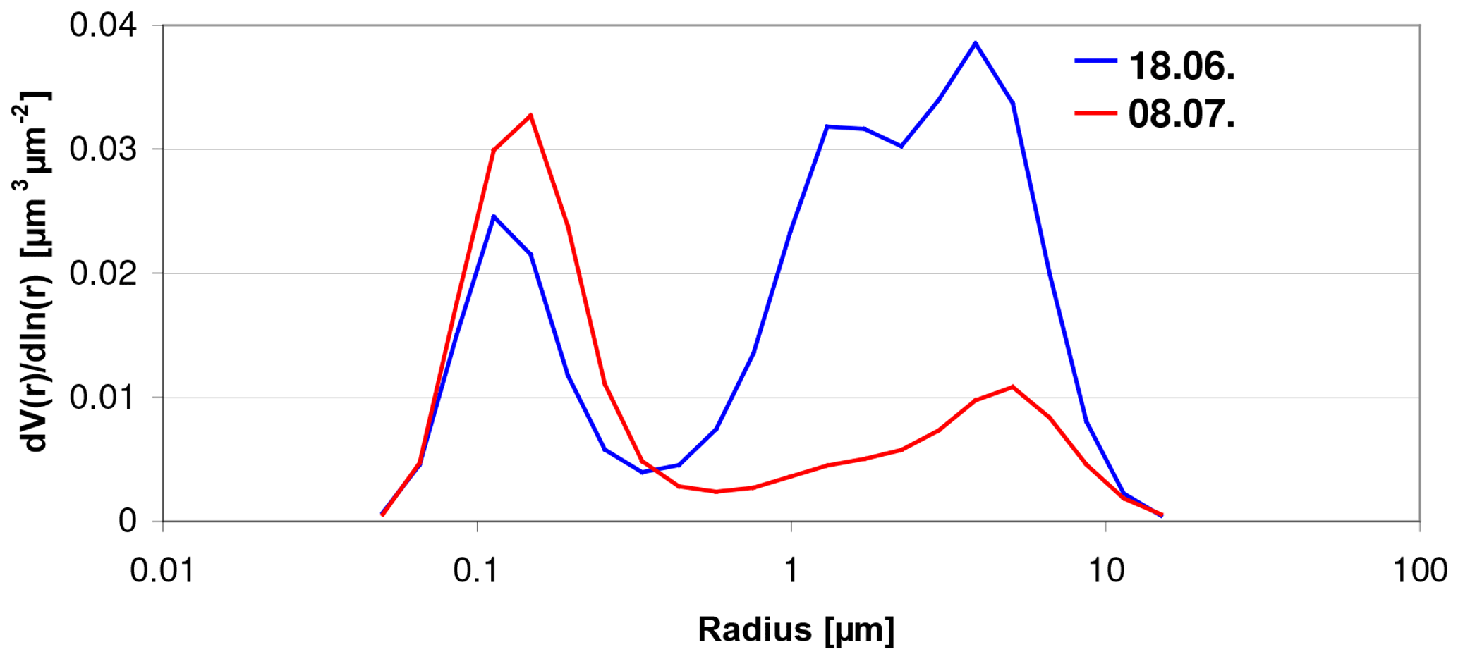
Figure A32Size distributions derived from AERONET Almucantar observations on 18 June (07:24 and 15:34) and 8 July (07:32 and 15:38).
Table A27Contributions of the coarse mode to the total AOD at different wavelengths derived from AERONET observations. The relative contributions are calculated assuming that the AOD of the coarse mode at 500 nm (0.093 and 0.010 on 18 June and 8 July, respectively) does not depend on wavelength.
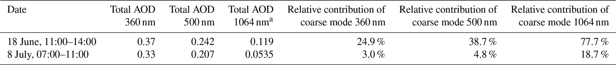
a This value was extrapolated from the measurements at 675 and 1020 nm.
It is found that on 18 June the coarse mode clearly dominates the AOD at 1064 nm, whereas on 8 July it only contributes about 20 % to the total AOD. As expected, the relative contributions of the coarse mode to the AOD at 360 nm are much smaller (25 % and 3 % on 18 June and 8 July, respectively).
In the last step the probability of aerosol scattering in the backward direction is considered, because the ceilometer receives scattered light from that direction. For that purpose the ratios of the optical depths are multiplied by the corresponding values of the normalised phase functions at 180∘ and in this way the relative contributions to the backscattered signals from the coarse mode for both wavelengths and both days are calculated (Table A28). Interestingly, on 8 July the contributions of the coarse mode to the backscattered signal at both wavelengths differ by only about 10 %. In contrast, on 18 June the difference is much larger.
Table A28Ratios of phase functions (coarse∕fine) in exactly backward direction and the relative contribution of coarse mode to the backscattered signal at both wavelengths.
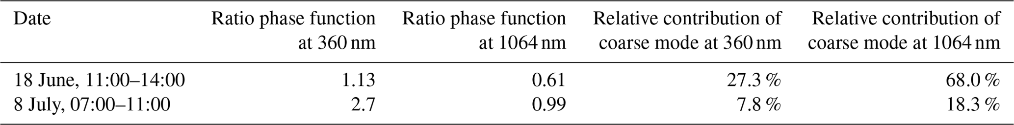
For 8 July, the results can be interpreted in the following way: at 360 nm the aerosol profiles extracted as described above overestimate the contribution from the coarse mode by about 10 %. To estimate the effect of this overestimation we construct modified aerosol extinction profiles, in which 10 % of the total AOD is relocated. Since we expect that the coarse-mode aerosols are usually located at low altitude, we construct four different modified profiles (see Fig. A33) with different altitudes (1.5, 1, 0.75, or 0.5 km), below which 10 % of the aerosol extinction is relocated to altitudes above (assuming that the coarse-mode aerosol is only located below these altitudes). Of course, such a sharp boundary is not very realistic, but it allows the overall effect of the relocation to be quantified. We selected the aerosol profile for 8 July extracted by INTA, which reached up to 7 km (see Fig. 9). It should be noted that if 10 % of the total AOD is relocated from the lowest layer to only the uppermost layer no further enhancement of the O4 dAMF is found (see Appendix A6).
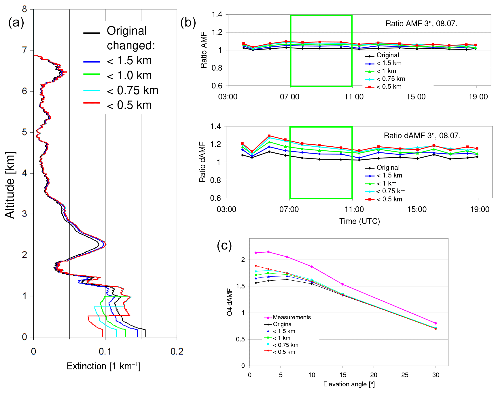
Figure A33(a) Modified aerosol profiles for 8 July assuming that the coarse-mode aerosol is only located in the lowest part of the atmosphere. (b) Ratios of the (d)AMFs calculated for the modified profiles compared to the dAMFs for the standard settings. With decreasing layer height the (d)AMFs increase systematically, because the aerosol extinction close to the surface decreases. (c) Comparison of the measured elevation dependence of the O4 dAMFs for the period 07:00–11:00 on 8 July and simulation results for the different profiles.
Table A29Ratios of the (d)AMFs for the modified profiles vs. those of the standard settings.
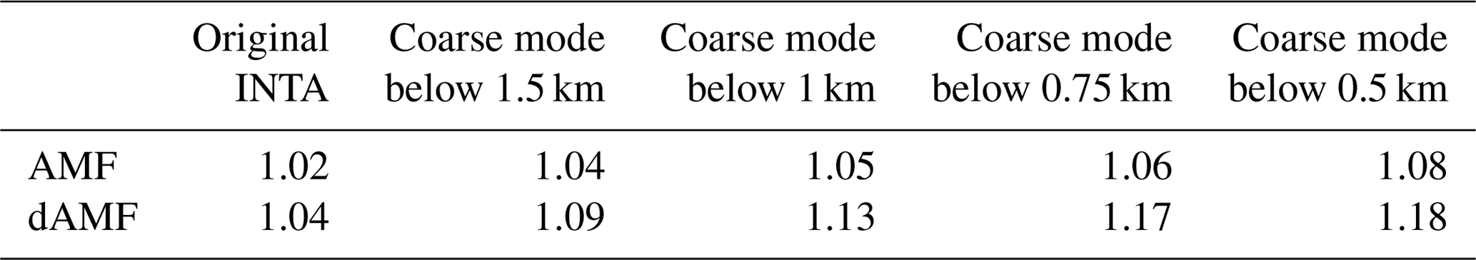
For all modified profiles, a systematic increase in the O4 (d)AMFs compared to those for the standard settings is found. For the O4 dAMFs this increase can be up to 18 % (see Table A29. From the comparison of the elevation dependence of the measured and simulated O4 dAMFs (see Fig. A33), we conclude that the aerosol profile with the coarse-mode aerosol below 0.75 km is probably the most realistic one. The main conclusion from this section is that the dAMF for 8 July derived from the standard settings probably underestimates the true dAMF by about 17±5 %.
For 18 June we did not perform similarly detailed calculations, because on that day the uncertainties of the aerosol extinction profile caused by the missing sensitivity of the ceilometer below 180 m are much larger than on 8 July. On 18 June the magnitude of the relocation of the aerosol extinction between different altitudes would also be much larger than on 8 July.
A6 Influence of elevated aerosol layers on the O4 (d)AMF
Ortega et al. (2016) showed that for their measurements the consideration of elevated aerosol layers (between about 3 and 5 km) is essential to bring measured and simulated O4 (d)AMFs into agreement. They also used lidar measurements at similar wavelengths as the MAX-DOAS observations. In our study, we consider aerosol layers over an even larger altitude range (up to 7 km). Nevertheless, it is interesting to see how the simulated O4 (d)AMFs change if the extinctions at various altitude ranges are changed systematically. Here we chose the aerosol extinction profile extracted by INTA for the period 07:00 to 11:00 on 8 July, because it contains substantial amounts of aerosols in elevated layers (see Fig. 9). During that period three distinct aerosol layers can be identified (see Table A30).
Table A30Selection of different aerosol layers on 8 July (07:00–11:00).
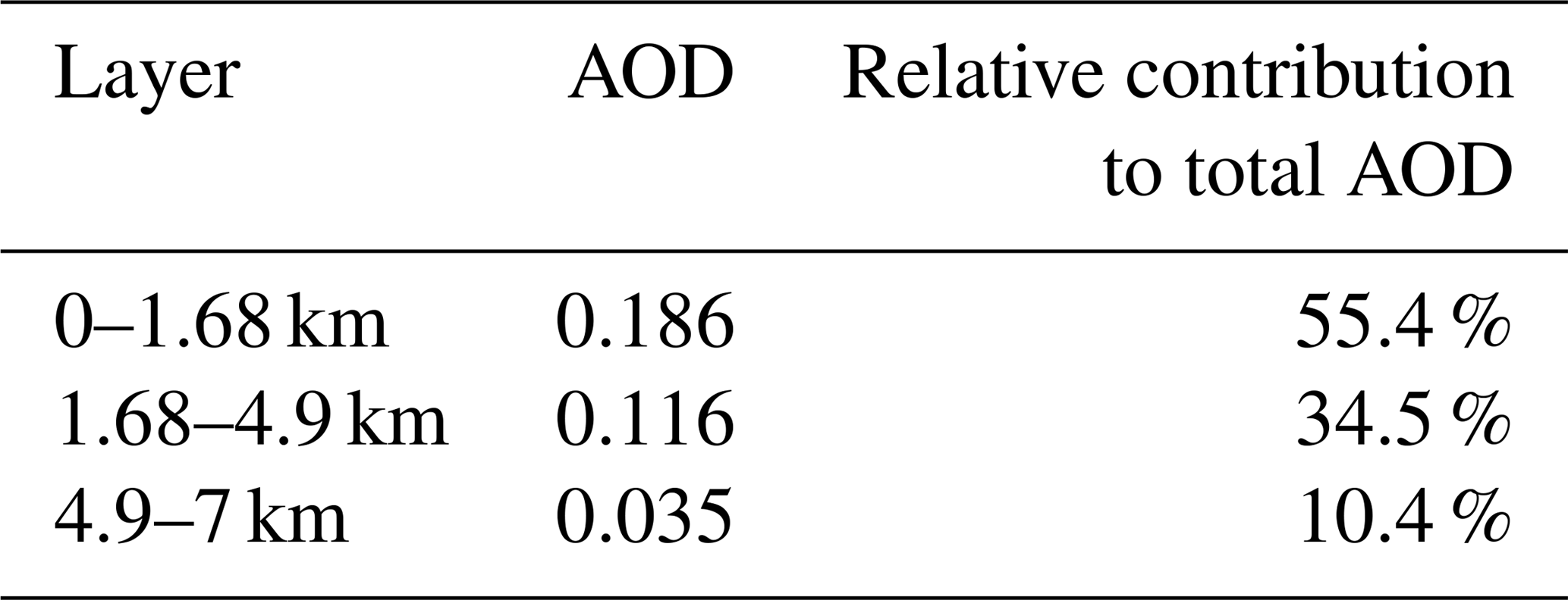
Then, the extinction of the individual aerosol layers was increased by 40 % compared to the original profile. After that modification the whole profiles are scaled with a constant factor to match the AOD of the sun photometer observations. The modified profiles are then used for the simulation of O4 (d)AMFs. A second set of profiles was created to investigate the effect of extreme relocations: here certain fractions (10 %, 25 % or 30 %) of the total AOD were relocated from the bottom layer to the top layer.
The modified profiles and the ratios of the corresponding O4 (d)AMFs vs. the O4 dAMFs of the original profile are shown in Fig. A34. For the O4 AMFs the relocations of the extinction profiles lead to a general increase in the O4 AMFs of up to 20 %. For the O4 dAMFs for most modified profiles a strong increase is found compared to the original profile. Only for the profile with an increase in the extinction in the lowest layer a slight decrease is observed. For the profiles with the extreme relocations the increase in the O4 dAMFs almost reaches 50 %.
From these results it can be concluded that for a relocation of about 27 % almost perfect agreement with the measurements is found (see Fig. A34). For such an aerosol profile simulations and measurements could be brought into agreement without a scaling factor. However, such a large redistribution is not supported by the AERONET inversion products (see Appendix A5). It should also be noted that for such a profile, about 73 % of the total AOD would be located above about 1.7 km. Moreover, for such an aerosol profile it is found that the simulated O4 AMFs for 90∘ elevation systematically underestimate the measured O4 AMFs at high SZA by about 15 % (see Fig. A34), whereas much better agreement is found for the standard settings. The underestimation of the O4 AMFs for 90∘ elevation is caused by the high aerosol amount at high altitudes, which increases the scattering altitude of the solar photons observed at 90∘ elevation. A similar effect could be caused by cirrus clouds, but on the selected days there are no indications of such clouds in the ceilometer data.
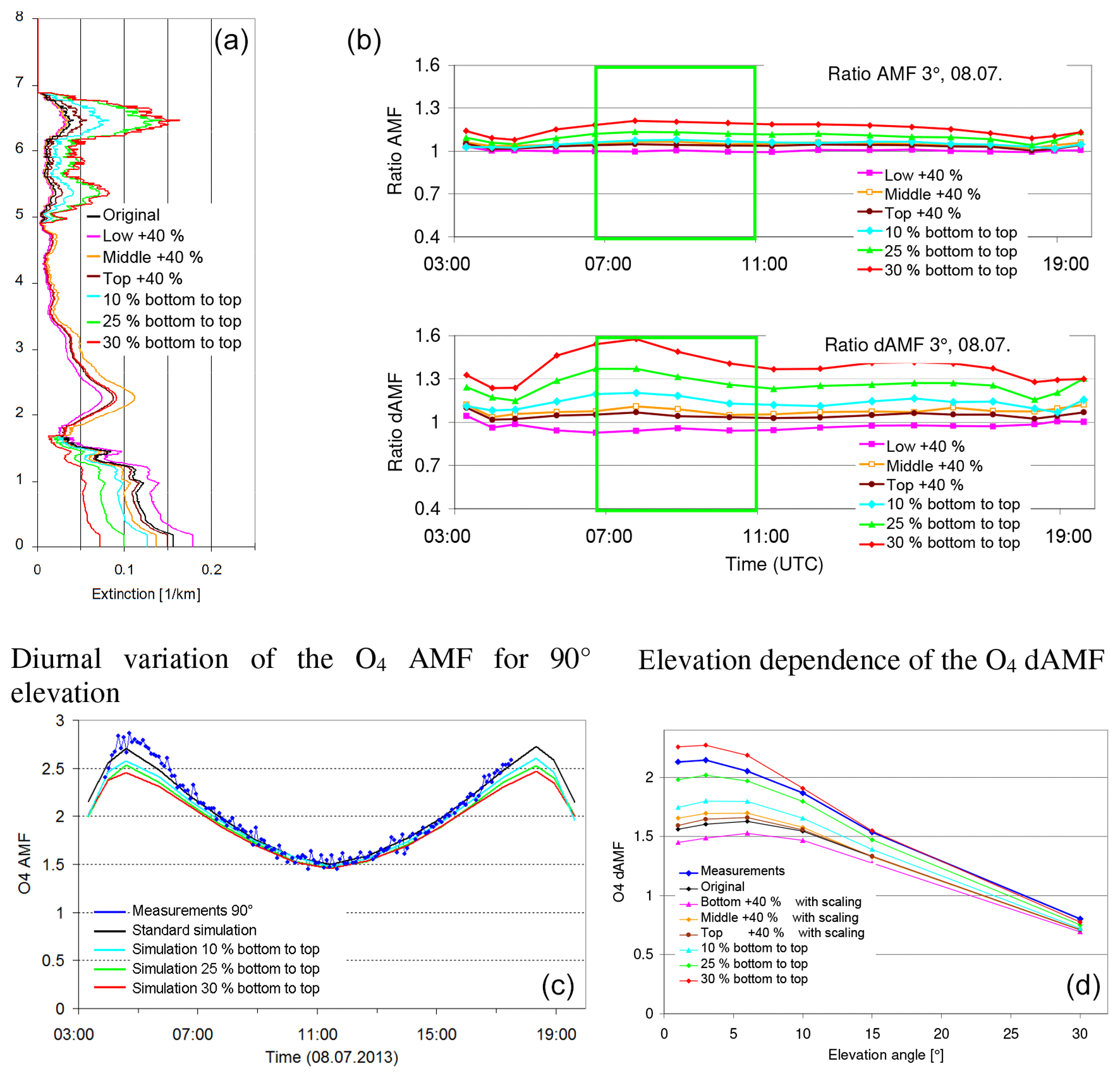
Figure A34(a) Aerosol profiles used for the simulations (see text). (b) Ratios of the O4 (d)AMFs simulated for the modified profiles vs. those of the original profile. (c, d) Comparison of the measured diurnal variation (SZA dependence) for 90∘ elevation (c) and the elevation dependence of the O4 dAMFs for the period 07:00–11:00 on 8 July (d).
Table A31Ratios of (d)AMFs for 8 July 2013 for the modified profiles with respect to the original profile.
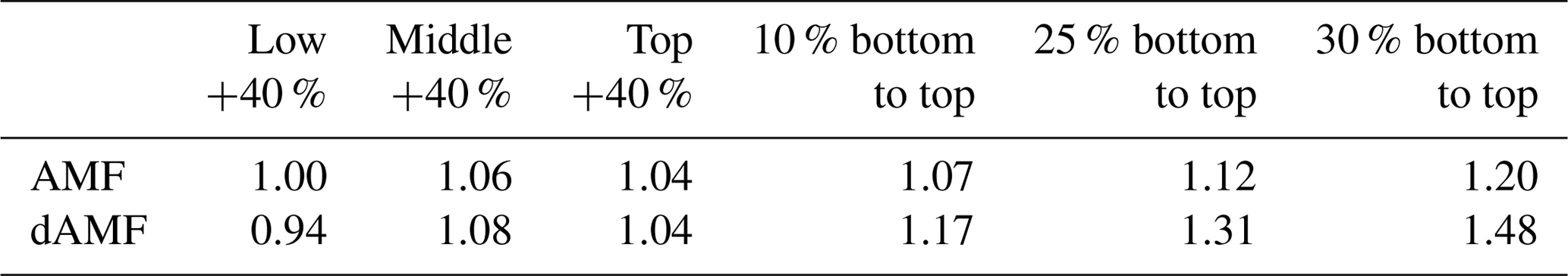
The authors declare that they have no conflict of interest.
We are thankful for several external data sets which were used in this
study: temperature and pressure profiles from the ERA-Interim reanalysis data
set were provided by the European Centre for Medium-Range Weather Forecasts.
In situ measurements of trace gas and aerosol concentrations, as well as
meteorological data, were performed by the environmental monitoring services
of the states of Rhineland-Palatinate and Hesse (http://www.luft-rlp.de, last access: 29 April 2019 and
https://www.hlnug.de/themen/luft/luftmessnetz.html, last access: 29 April 2019).
We thank Meinrat O. Andreae
and Günther Schebeske for operating the ceilometer and the AERONET
instrument at the Max Planck Institute for Chemistry. We also would like to
thank Rainer Volkamer, Theodore K. Koenig and Ivan Ortega for their very helpful
comments.
The article processing charges for this open-access
publication were covered by the Max Planck Society.
This paper was edited by Jochen Stutz and reviewed by two anonymous referees.
Acarreta, J. R., De Haan, J. F., and Stammes, P.: Cloud pressure retrieval using the O2-O2 absorption band at 477 nm, J. Geophys. Res., 109, D05204, https://doi.org/10.1029/2003JD003915, 2004.
Bogumil, K., Orphal, J., Homann, T., Voigt, S., Spietz, P., Fleischmann, O. C., Vogel, A., Hartmann, M., Bovensmann, H., Frerik, J., and Burrows, J. P.: Measurements of Molecular Absorption Spectra with the SCIAMACHY Pre-Flight Model: Instrument Characterization and Reference Data for Atmospheric Remote-Sensing in the 230–2380 nm Region, J. Photochem. Photobiol. A., 157, 167–184, 2003.
Chance, K. V. and Kurucz, R. L.: An improved high-resolution solar reference spectrum for earth's atmosphere measurements in the ultraviolet, visible, and near infrared, J. Quant. Spectrosc. Ra., 111, 1289–1295, 2010.
Chandrasekhar, S.: Radiative Transfer, Dover Publications Inc., New York, 1960.
Chandrasekhar, S.: Selected papers, vol. 2, University of Chicago Press, New York, 1989.
Clémer, K., Van Roozendael, M., Fayt, C., Hendrick, F., Hermans, C., Pinardi, G., Spurr, R., Wang, P., and De Mazière, M.: Multiple wavelength retrieval of tropospheric aerosol optical properties from MAXDOAS measurements in Beijing, Atmos. Meas. Tech., 3, 863–878, https://doi.org/10.5194/amt-3-863-2010, 2010.
Dee, D. P., Uppala, S. M., Simmons, A. J., Berrisford, P., Poli, P., Kobayashi, S., Andrae, U., Balmaseda, M. A., Balsamo, G., Bauer, P., Bechtold, P., Beljaars, A. C. M., van de Berg, L., Bidlot, J., Bormann, N., Delsol, C., Dragani, R., Fuentes, M., Geer, A. J., Haimberger, L., Healy, S. B., Hersbach, H., Hólm, E. V., Isaksen, L., Kållberg, P., Köhler, M., Matricardi, M., McNally, A. P., Monge-Sanz, B. M., Morcrette, J.-J., Park, B.-K., Peubey, C., de Rosnay, P., Tavolato, C., Thépaut, J.-N., and Vitart, F.: The ERA-Interim reanalysis: configuration and performance of the data assimilation system, Q. J. Roy. Meteor. Soc., 137, 553–597, https://doi.org/10.1002/qj.828, 2011.
Deutschmann, T., Beirle, S., Frieß, U., Grzegorski, M., Kern, C., Kritten, L., Platt, U., Puķīte, J., Wagner, T., Werner, B., and Pfeilsticker, K.: The Monte Carlo Atmospheric Radiative Transfer Model McArtim: Introduction and Validation of Jacobians and 3D Features, J. Quant. Spectrosc. Ra., 112, 1119–1137, https://doi.org/10.1016/j.jqsrt.2010.12.009, 2011.
Dubovik, O., Holben, B. N., Eck, T. F., Smirnov, A., Kaufman, Y. J., King, M. D., Tanré, D., and Slutsker, I.: Variability of absorption and optical properties of key aerosol types observed in worldwide locations, J. Atmos. Sci., 59, 590–608, 2002.
Erle, F., Pfeilsticker, K., and Platt, U.: On the influence of tropospheric clouds on zenith-scattered-light measurements of stratospheric species, Geophys. Res. Lett., 22, 2725–2728, 1995.
Fleischmann, O. C., Hartmann, M., Burrows, J. P., and Orphal, J.: New ultraviolet absorption cross-sections of BrO at atmospheric temperatures measured by time-windowing Fourier transform spectroscopy, J. Photoch. Photobio. A, 168, 117–132, 2004.
Franco, B., Hendrick, F., Van Roozendael, M., Müller, J.-F., Stavrakou, T., Marais, E. A., Bovy, B., Bader, W., Fayt, C., Hermans, C., Lejeune, B., Pinardi, G., Servais, C., and Mahieu, E.: Retrievals of formaldehyde from ground-based FTIR and MAX-DOAS observations at the Jungfraujoch station and comparisons with GEOS-Chem and IMAGES model simulations, Atmos. Meas. Tech., 8, 1733–1756, https://doi.org/10.5194/amt-8-1733-2015, 2015.
Frieß, F., Monks, P. S., Remedios, J. J., Rozanov, A., Sinreich, R., Wagner, T., and Platt, U.: MAX-DOAS O4 measurements: A new technique to derive information on atmospheric aerosols. (II) Modelling studies, J. Geophys. Res., 111, D14203, https://doi.org/10.1029/2005JD006618, 2006.
Frieß, U., Sihler, H., Sander, R., Pöhler, D., Yilmaz, S., and Platt, U.: The vertical distribution of BrO and aerosols in the Arctic: measurements by active and passive differential optical absorption sprectroscopy, J. Geophys. Res., 116, D00R04, https://doi.org/10.1029/2011JD015938, 2011.
Frieß, U., Klein Baltink, H., Beirle, S., Clémer, K., Hendrick, F., Henzing, B., Irie, H., de Leeuw, G., Li, A., Moerman, M. M., van Roozendael, M., Shaiganfar, R., Wagner, T., Wang, Y., Xie, P., Yilmaz, S., and Zieger, P.: Intercomparison of aerosol extinction profiles retrieved from MAX-DOAS measurements, Atmos. Meas. Tech., 9, 3205–3222, https://doi.org/10.5194/amt-9-3205-2016, 2016.
Gielen, C., Van Roozendael, M., Hendrick, F., Pinardi, G., Vlemmix, T., De Bock, V., De Backer, H., Fayt, C., Hermans, C., Gillotay, D., and Wang, P.: A simple and versatile cloud-screening method for MAX-DOAS retrievals, Atmos. Meas. Tech., 7, 3509–3527, https://doi.org/10.5194/amt-7-3509-2014, 2014.
Gielen, C., Hendrick, F., Pinardi, G., De Smedt, I., Fayt, C., Hermans, C., Stavrakou, T., Bauwens, M., Müller, J.-F., Ndenzako, E., Nzohabonayo, P., Akimana, R., Niyonzima, S., Van Roozendael, M., and De Mazière, M.: Characterisation of Central-African aerosol and trace-gas emissions based on MAX-DOAS measurements and model simulations over Bujumbura, Burundi, Atmos. Chem. Phys. Discuss., https://doi.org/10.5194/acp-2016-1104, in review, 2017.
Greenblatt, G. D., Orlando, J. J., Burkholder, J. B., and Ravishankara, A. R.: Absorption measurements of oxygen between 330 and 1140 nm, J. Geophys. Res., 95, 18577–18582, 1990.
Hendrick, F., Van Roozendael, M., Kylling, A., Petritoli, A., Rozanov, A., Sanghavi, S., Schofield, R., von Friedeburg, C., Wagner, T., Wittrock, F., Fonteyn, D., and De Mazière, M.: Intercomparison exercise between different radiative transfer models used for the interpretation of ground-based zenith-sky and multi-axis DOAS observations, Atmos. Chem. Phys., 6, 93–108, https://doi.org/10.5194/acp-6-93-2006, 2006.
Hendrick, F., Müller, J.-F., Clémer, K., Wang, P., De Mazière, M., Fayt, C., Gielen, C., Hermans, C., Ma, J. Z., Pinardi, G., Stavrakou, T., Vlemmix, T., and Van Roozendael, M.: Four years of ground-based MAX-DOAS observations of HONO and NO2 in the Beijing area, Atmos. Chem. Phys., 14, 765–781, https://doi.org/10.5194/acp-14-765-2014, 2014.
Heue, K.-P., Riede, H., Walter, D., Brenninkmeijer, C. A. M., Wagner, T., Frieß, U., Platt, U., Zahn, A., Stratmann, G., and Ziereis, H.: CARIBIC DOAS observations of nitrous acid and formaldehyde in a large convective cloud, Atmos. Chem. Phys., 14, 6621–6642, https://doi.org/10.5194/acp-14-6621-2014, 2014.
Holben, B. N., Tanre, D., Smirnov, A., Eck, T. F., Slutsker, I., Abuhassan, N., Newcomb, W. W., Schafer, J., Chatenet, B., Lavenue, F., Kaufman, Y. J., Vande Castle, J., Setzer, A., Markham, B., Clark, D., Frouin, R., Halthore, R., Karnieli, A., O'Neill, N. T., Pietras, C., Pinker, R. T., Voss, K., and Zibordi, G.: An emerging ground-based aerosol climatology: Aerosol Optical Depth from AERONET, J. Geophys. Res., 106, 12067–12097, 2001.
Hönninger, G., von Friedeburg, C., and Platt, U.: Multi axis differential optical absorption spectroscopy (MAX-DOAS), Atmos. Chem. Phys., 4, 231–254, https://doi.org/10.5194/acp-4-231-2004, 2004.
Irie, H., Kanaya, Y., Akimoto, H., Iwabuchi, H., Shimizu, A., and Aoki, K.: First retrieval of tropospheric aerosol profiles using MAX-DOAS and comparison with lidar and sky radiometer measurements, Atmos. Chem. Phys., 8, 341–350, https://doi.org/10.5194/acp-8-341-2008, 2008.
Irie, H., Takashima, H., Kanaya, Y., Boersma, K. F., Gast, L., Wittrock, F., Brunner, D., Zhou, Y., and Van Roozendael, M.: Eight-component retrievals from ground-based MAX-DOAS observations, Atmos. Meas. Tech., 4, 1027–1044, https://doi.org/10.5194/amt-4-1027-2011, 2011.
Irie, H., Nakayama, T., Shimizu, A., Yamazaki, A., Nagai, T., Uchiyama, A., Zaizen, Y., Kagamitani, S., and Matsumi, Y.: Evaluation of MAX-DOAS aerosol retrievals by coincident observations using CRDS, lidar, and sky radiometer in Tsukuba, Japan, Atmos. Meas. Tech., 8, 2775–2788, https://doi.org/10.5194/amt-8-2775-2015, 2015.
Kanaya, Y., Irie, H., Takashima, H., Iwabuchi, H., Akimoto, H., Sudo, K., Gu, M., Chong, J., Kim, Y. J., Lee, H., Li, A., Si, F., Xu, J., Xie, P.-H., Liu, W.-Q., Dzhola, A., Postylyakov, O., Ivanov, V., Grechko, E., Terpugova, S., and Panchenko, M.: Long-term MAX-DOAS network observations of NO2 in Russia and Asia (MADRAS) during the period 2007–2012: instrumentation, elucidation of climatology, and comparisons with OMI satellite observations and global model simulations, Atmos. Chem. Phys., 14, 7909–7927, https://doi.org/10.5194/acp-14-7909-2014, 2014.
Krautwurst, S.: Charakterisierung eines neu aufgebauten MAXDOAS-Systems und Interpretation von ersten Messergebnissen zu dem Spurenstoff NO2, Diplomarbeit, Fachhochschule Coburg, Coburg, Germany, 2010.
Kreher, K., Van Roozendael, M., Hendrick, F., Apituley, A., Dimitropoulou, E., Friess, U., Richter, A., Wagner, T., Ang, L., Anguas, M., Bais, A., Benavent, N., Bognar, K., Borovski, A., Bruchkovsky, I., Cede, A., Chan, K. L., Donner, S., Drosoglou, T., Fayt, C., Finkenzeller, H., Hao, N., Hermans, C., Hoque, S., Irie, H., Jin, J., Johnston, P., Khayyam Butt, J., Khokhar, F., Koenig, T., Ma, J., Mishra, A. K., Navarro-Comas, M., Pazmino, A., Peters, E., Pinharanda, M., Piters, A., Postylyakov, O., Prados, C., Rodriguez, O., Querel, R., Saiz-Lopez, A., Schreier, S., Seyler, A., Spinei, E., Strong, K., Tiefengraber, M., Tirpitz, J.-L., Kumar, V., Volkamer, R., Wenig, M., Xie, P., Xu, J., Yela, M., Zhao, X., and Zhuoru, W.: Intercomparison of NO2, O4, O3 and HCHO slant column measurements by MAX-DOAS and zenith-sky UV-Visible spectrometers, Atmos. Meas. Tech. Discuss., submitted, 2019.
Lampel, J., Frieß, U., and Platt, U.: The impact of vibrational Raman scattering of air on DOAS measurements of atmospheric trace gases, Atmos. Meas. Tech., 8, 3767–3787, https://doi.org/10.5194/amt-8-3767-2015, 2015.
Lampel, J., Pöhler, D., Polyansky, O. L., Kyuberis, A. A., Zobov, N. F., Tennyson, J., Lodi, L., Frieß, U., Wang, Y., Beirle, S., Platt, U., and Wagner, T.: Detection of water vapour absorption around 363 nm in measured atmospheric absorption spectra and its effect on DOAS evaluations, Atmos. Chem. Phys., 17, 1271–1295, https://doi.org/10.5194/acp-17-1271-2017, 2017.
Lorente, A., Folkert Boersma, K., Yu, H., Dörner, S., Hilboll, A., Richter, A., Liu, M., Lamsal, L. N., Barkley, M., De Smedt, I., Van Roozendael, M., Wang, Y., Wagner, T., Beirle, S., Lin, J.-T., Krotkov, N., Stammes, P., Wang, P., Eskes, H. J., and Krol, M.: Structural uncertainty in air mass factor calculation for NO2 and HCHO satellite retrievals, Atmos. Meas. Tech., 10, 759–782, https://doi.org/10.5194/amt-10-759-2017, 2017.
Meller, R. and Moortgat, G. K.: Temperature dependence of the absorption cross sections of formaldehyde between 223 and 323 K in the wavelength range 225–375 nm, J. Geophys. Res., 105, 7089–7101, 2000.
Merlaud, A., Van Roozendael, M., Theys, N., Fayt, C., Hermans, C., Quennehen, B., Schwarzenboeck, A., Ancellet, G., Pommier, M., Pelon, J., Burkhart, J., Stohl, A., and De Mazière, M.: Airborne DOAS measurements in Arctic: vertical distributions of aerosol extinction coefficient and NO2 concentration, Atmos. Chem. Phys., 11, 9219–9236, https://doi.org/10.5194/acp-11-9219-2011, 2011.
Ortega, I., Berg, L. K., Ferrare, R. A., Hair, J. W., Hostetler, C. A., and Volkamer, R.: Elevated aerosol layers modify the O2-O2 absorption measured by ground-based MAX-DOAS, J. Quant. Spectrosc. Ra., 176, 34–49, https://doi.org/10.1016/j.jqsrt.2016.02.021, 2016.
Paur, R. J. and Bass, A. M.: The Ultraviolet Cross-Sections of Ozone: II. Results and temperature dependence, in: Atmospheric ozone, edited by: Zeferos, C. S. and Ghazi, A., Proc. Quadrennial Ozone Symposium, Halkidiki Greece, 1984, Reidel, D., Dordrecht, 611–615, 1984.
Peters, E., Wittrock, F., Großmann, K., Frieß, U., Richter, A., and Burrows, J. P.: Formaldehyde and nitrogen dioxide over the remote western Pacific Ocean: SCIAMACHY and GOME-2 validation using ship-based MAX-DOAS observations, Atmos. Chem. Phys., 12, 11179–11197, https://doi.org/10.5194/acp-12-11179-2012, 2012.
Pinardi, G., Van Roozendael, M., Abuhassan, N., Adams, C., Cede, A., Clémer, K., Fayt, C., Frieß, U., Gil, M., Herman, J., Hermans, C., Hendrick, F., Irie, H., Merlaud, A., Navarro Comas, M., Peters, E., Piters, A. J. M., Puentedura, O., Richter, A., Schönhardt, A., Shaiganfar, R., Spinei, E., Strong, K., Takashima, H., Vrekoussis, M., Wagner, T., Wittrock, F., and Yilmaz, S.: MAX-DOAS formaldehyde slant column measurements during CINDI: intercomparison and analysis improvement, Atmos. Meas. Tech., 6, 167–185, https://doi.org/10.5194/amt-6-167-2013, 2013.
Polyansky, O. L., Kyuberis, A. A., Zobov, N. F., Tennyson, J., Yurchenko, S. N., and Lodi, L.: ExoMol molecular line lists XXX: a complete high-accuracy line list for water, Mon. Not. R. Astron. Soc., 480, 2597–2608, 2018.
Prados-Roman, C., Butz, A., Deutschmann, T., Dorf, M., Kritten, L., Minikin, A., Platt, U., Schlager, H., Sihler, H., Theys, N., Van Roozendael, M., Wagner, T., and Pfeilsticker, K.: Airborne DOAS limb measurements of tropospheric trace gas profiles: case studies on the profile retrieval of O4 and BrO, Atmos. Meas. Tech., 4, 1241–1260, https://doi.org/10.5194/amt-4-1241-2011, 2011.
Puķīte, J., Kühl, S., Deutschmann, T., Platt, U., and Wagner, T.: Extending differential optical absorption spectroscopy for limb measurements in the UV, Atmos. Meas. Tech., 3, 631–653, https://doi.org/10.5194/amt-3-631-2010, 2010.
Rozanov, V. V., Rozanov, A. V., Kokhanovsky, A. A., and Burrows, J. P.: Radiative transfer through terrestrial atmosphere and ocean: Software package SCIATRAN, J. Quant. Spectrosc. Ra., 133, 13-71, 2014.
Schreier, S. F., Richter, A., Wittrock, F., and Burrows, J. P.: Estimates of free-tropospheric NO2 and HCHO mixing ratios derived from high-altitude mountain MAX-DOAS observations at midlatitudes and in the tropics, Atmos. Chem. Phys., 16, 2803–2817, https://doi.org/10.5194/acp-16-2803-2016, 2016.
Serdyuchenko, A., Gorshelev, V., Weber, M., Chehade, W., and Burrows, J. P.: High spectral resolution ozone absorption cross-sections – Part 2: Temperature dependence, Atmos. Meas. Tech., 7, 625–636, https://doi.org/10.5194/amt-7-625-2014, 2014.
Seyler, A., Wittrock, F., Kattner, L., Mathieu-Üffing, B., Peters, E., Richter, A., Schmolke, S., and Burrows, J. P.: Monitoring shipping emissions in the German Bight using MAX-DOAS measurements, Atmos. Chem. Phys., 17, 10997–11023, https://doi.org/10.5194/acp-17-10997-2017, 2017.
Sneep, M., de Haan, J. F., Stammes, P., Wang, P., Vanbauce, C., Joiner, J., Vasilkov, A. P., and Levelt, P. F.: Three-way comparison between OMI and PARASOL cloud pressure products, J. Geophys. Res., 113, D15S23, https://doi.org/10.1029/2007JD008694, 2008.
Solomon, S., Schmeltekopf, A. L., and Sanders, R. W.: On the interpretation of zenith sky absorption measurements, J. Geophys. Res., 92, 8311–8319, 1987.
Spinei, E., Cede, A., Herman, J., Mount, G. H., Eloranta, E., Morley, B., Baidar, S., Dix, B., Ortega, I., Koenig, T., and Volkamer, R.: Ground-based direct-sun DOAS and airborne MAX-DOAS measurements of the collision-induced oxygen complex, O2–O2, absorption with significant pressure and temperature differences, Atmos. Meas. Tech., 8, 793–809, https://doi.org/10.5194/amt-8-793-2015, 2015.
Spurr, R.: LIDORT and VLIDORT: Linearized Pseudo-Spherical Scalar and Vector Discrete Ordinate Radiative Transfer Models for Use in Remote Sensing Retrieval Problems, Light Scattering Reviews, vol. 3, edited by: Kokhanovsky, A., Springer, Berlin Heidelberg, Germany, 2008.
Spurr, R. J. D., Kurosu, T. P., and Chance, K. V.: A linearized discrete ordinate radiative transfer model for atmospheric remote sensing retrieval, J. Quant. Spectrosc. Ra., 68, 689–735, 2001.
Stamnes, K., Tsay, S.-C., Wiscombe, W., and Jayaweera, K.: Numerically stable algorithm for discrete ordinate method radiative transfer in multiple scattering and emitting layered media, Appl Optics, 27, 2502–2509, 1988.
Thalman, R. and Volkamer, R.: Inherent calibration of a blue LED-CE-DOAS instrument to measure iodine oxide, glyoxal, methyl glyoxal, nitrogen dioxide, water vapour and aerosol extinction in open cavity mode, Atmos. Meas. Tech., 3, 1797–1814, https://doi.org/10.5194/amt-3-1797-2010, 2010.
Thalman, R. and Volkamer, R.: Temperature dependent absorption cross-sections of O2–O2 collision pairs between 340 and 630 nm and at atmospherically relevant pressure, Phys. Chem. Chem. Phys., 15, 15371, https://doi.org/10.1039/c3cp50968k, 2013.
United States Committee on Extension to the Standard Atmosphere: U.S. Standard Atmosphere, 1976, National Oceanic and Atmospheric Administration, National Aeronautics and Space Administration, United States Air Force, Washington D.C., 1976.
Vandaele, A. C., Hermans, C., Simon, P. C., Carleer, M., Colin, R., Fally, S., Mérienne, M.-F., Jenouvrier, A., and Coquart, B.: Measurements of the NO2 Absorption Cross-section from 42 000 cm−1 to 10 000 cm−1 (238–1000 nm) at 220 K and 294 K, J. Quant. Spectrosc. Ra., 59, 171–184, 1997.
Vlemmix, T., Piters, A. J. M., Berkhout, A. J. C., Gast, L. F. L., Wang, P., and Levelt, P. F.: Ability of the MAX-DOAS method to derive profile information for NO2: can the boundary layer and free troposphere be separated?, Atmos. Meas. Tech., 4, 2659–2684, https://doi.org/10.5194/amt-4-2659-2011, 2011.
Vlemmix, T., Hendrick, F., Pinardi, G., De Smedt, I., Fayt, C., Hermans, C., Piters, A., Wang, P., Levelt, P., and Van Roozendael, M.: MAX-DOAS observations of aerosols, formaldehyde and nitrogen dioxide in the Beijing area: comparison of two profile retrieval approaches, Atmos. Meas. Tech., 8, 941–963, https://doi.org/10.5194/amt-8-941-2015, 2015.
Volkamer, R., Baidar, S., Campos, T. L., Coburn, S., DiGangi, J. P., Dix, B., Eloranta, E. W., Koenig, T. K., Morley, B., Ortega, I., Pierce, B. R., Reeves, M., Sinreich, R., Wang, S., Zondlo, M. A., and Romashkin, P. A.: Aircraft measurements of BrO, IO, glyoxal, NO2, H2O, O2–O2 and aerosol extinction profiles in the tropics: comparison with aircraft-/ship-based in situ and lidar measurements, Atmos. Meas. Tech., 8, 2121–2148, https://doi.org/10.5194/amt-8-2121-2015, 2015.
Wagner, T., Erle, F., Marquard, L., Otten, C., Pfeilsticker, K., Senne, T., Stutz, J., and Platt, U.: Cloudy sky optical paths as derived from differential optical absorption spectroscopy observations, J. Geophys. Res., 103, 25307–25321, 1998.
Wagner, T., Dix, B., von Friedeburg, C., Frieß, U., Sanghavi, S., Sinreich, R., and Platt, U.: MAX-DOAS O4 measurements – a new technique to derive information on atmospheric aerosols. (I) Principles and information content, J. Geophys. Res., 109, D22205, https://doi.org/10.1029/2004JD004904, 2004.
Wagner, T., Burrows, J. P., Deutschmann, T., Dix, B., von Friedeburg, C., Frieß, U., Hendrick, F., Heue, K.-P., Irie, H., Iwabuchi, H., Kanaya, Y., Keller, J., McLinden, C. A., Oetjen, H., Palazzi, E., Petritoli, A., Platt, U., Postylyakov, O., Pukite, J., Richter, A., van Roozendael, M., Rozanov, A., Rozanov, V., Sinreich, R., Sanghavi, S., and Wittrock, F.: Comparison of box-air-mass-factors and radiances for Multiple-Axis Differential Optical Absorption Spectroscopy (MAX-DOAS) geometries calculated from different UV/visible radiative transfer models, Atmos. Chem. Phys., 7, 1809–1833, https://doi.org/10.5194/acp-7-1809-2007, 2007.
Wagner, T., Deutschmann, T., and Platt, U.: Determination of aerosol properties from MAX-DOAS observations of the Ring effect, Atmos. Meas. Tech., 2, 495–512, https://doi.org/10.5194/amt-2-495-2009, 2009.
Wagner, T., Beirle, S., Deutschmann, T., and Penning de Vries, M.: A sensitivity analysis of Ring effect to aerosol properties and comparison to satellite observations, Atmos. Meas. Tech., 3, 1723–1751, https://doi.org/10.5194/amt-3-1723-2010, 2010.
Wagner, T., Apituley, A., Beirle, S., Dörner, S., Friess, U., Remmers, J., and Shaiganfar, R.: Cloud detection and classification based on MAX-DOAS observations, Atmos. Meas. Tech., 7, 1289–1320, https://doi.org/10.5194/amt-7-1289-2014, 2014.
Wang, S., Cuevas, C. A., Frieß, U., and Saiz-Lopez, A.: MAX-DOAS retrieval of aerosol extinction properties in Madrid, Spain, Atmos. Meas. Tech., 9, 5089–5101, https://doi.org/10.5194/amt-9-5089-2016, 2016.
Wang, T., Hendrick, F., Wang, P., Tang, G., Clémer, K., Yu, H., Fayt, C., Hermans, C., Gielen, C., Müller, J.-F., Pinardi, G., Theys, N., Brenot, H., and Van Roozendael, M.: Evaluation of tropospheric SO2 retrieved from MAX-DOAS measurements in Xianghe, China, Atmos. Chem. Phys., 14, 11149–11164, https://doi.org/10.5194/acp-14-11149-2014, 2014.
Wang, Y., Beirle, S., Hendrick, F., Hilboll, A., Jin, J., Kyuberis, A. A., Lampel, J., Li, A., Luo, Y., Lodi, L., Ma, J., Navarro, M., Ortega, I., Peters, E., Polyansky, O. L., Remmers, J., Richter, A., Puentedura, O., Van Roozendael, M., Seyler, A., Tennyson, J., Volkamer, R., Xie, P., Zobov, N. F., and Wagner, T.: MAX-DOAS measurements of HONO slant column densities during the MAD-CAT campaign: inter-comparison, sensitivity studies on spectral analysis settings, and error budget, Atmos. Meas. Tech., 10, 3719–3742, https://doi.org/10.5194/amt-10-3719-2017, 2017a.
Wang, Y., Beirle, S., Lampel, J., Koukouli, M., De Smedt, I., Theys, N., Li, A., Wu, D., Xie, P., Liu, C., Van Roozendael, M., Stavrakou, T., Müller, J.-F., and Wagner, T.: Validation of OMI, GOME-2A and GOME-2B tropospheric NO2, SO2 and HCHO products using MAX-DOAS observations from 2011 to 2014 in Wuxi, China: investigation of the effects of priori profiles and aerosols on the satellite products, Atmos. Chem. Phys., 17, 5007–5033, https://doi.org/10.5194/acp-17-5007-2017, 2017b.
Wang, Y., Lampel, J., Xie, P., Beirle, S., Li, A., Wu, D., and Wagner, T.: Ground-based MAX-DOAS observations of tropospheric aerosols, NO2, SO2 and HCHO in Wuxi, China, from 2011 to 2014, Atmos. Chem. Phys., 17, 2189–2215, https://doi.org/10.5194/acp-17-2189-2017, 2017c.
Wiegner, M. and Geiß, A.: Aerosol profiling with the Jenoptik ceilometer CHM15kx, Atmos. Meas. Tech., 5, 1953–1964, https://doi.org/10.5194/amt-5-1953-2012, 2012.
Winterrath, T., Kurosu, T. P., Richter, A., and Burrows, J. P.: Enhanced O3 and NO2 in thunderstorm clouds: convection or production?, Geophys. Res. Lett., 26, 1291–1294, 1999.
Wittrock, F., Oetjen, H., Richter, A., Fietkau, S., Medeke, T., Rozanov, A., and Burrows, J. P.: MAX-DOAS measurements of atmospheric trace gases in Ny-Ålesund – Radiative transfer studies and their application, Atmos. Chem. Phys., 4, 955–966, https://doi.org/10.5194/acp-4-955-2004, 2004.
Zieger, P., Weingartner, E., Henzing, J., Moerman, M., de Leeuw, G., Mikkilä, J., Ehn, M., Petäjä, T., Clémer, K., van Roozendael, M., Yilmaz, S., Frieß, U., Irie, H., Wagner, T., Shaiganfar, R., Beirle, S., Apituley, A., Wilson, K., and Baltensperger, U.: Comparison of ambient aerosol extinction coefficients obtained from in-situ, MAX-DOAS and LIDAR measurements at Cabauw, Atmos. Chem. Phys., 11, 2603–2624, https://doi.org/10.5194/acp-11-2603-2011, 2011.
- Abstract
- Introduction
- MAD-CAT campaign, MAX-DOAS instruments and other data sets used in this study
- Strategies used in this study and comparison results for the standard settings
- Estimation of the uncertainties of the different processing steps
- Comparison of measurements and simulations
- Conclusions
- Data availability
- Appendix A
- Competing interests
- Acknowledgements
- Review statement
- References