the Creative Commons Attribution 4.0 License.
the Creative Commons Attribution 4.0 License.
 | 29 May 2019
Quantification of CO2 and CH4 emissions over Sacramento, California, based on divergence theorem using aircraft measurements
Ju-Mee Ryoo
Laura T. Iraci
Tomoaki Tanaka
Josette E. Marrero
Emma L. Yates
Inez Fung
Anna M. Michalak
Jovan Tadić
Warren Gore
T. Paul Bui
Jonathan M. Dean-Day
Cecilia S. Chang
Emission estimates of carbon dioxide (CO2) and methane (CH4) and the meteorological factors affecting them are investigated over Sacramento, California, using an aircraft equipped with a cavity ring-down greenhouse gas sensor as part of the Alpha Jet Atmospheric eXperiment (AJAX) project. To better constrain the emission fluxes, we designed flights in a cylindrical pattern and computed the emission fluxes from two flights using a kriging method and Gauss's divergence theorem.
Differences in wind treatment and assumptions about background concentrations affect the emission estimates by a factor of 1.5 to 7. The uncertainty is also impacted by meteorological conditions and distance from the emission sources. The vertical layer averaging affects the flux estimate, but the choice of raw wind or mass-balanced wind is more important than the thickness of the vertical averaging for mass-balanced wind for both urban and local scales.
The importance of vertical mass transfer for flux estimates is examined, and the difference in the total emission estimate with and without vertical mass transfer is found to be small, especially at the local scale. The total flux estimates accounting for the entire circumference are larger than those based solely on measurements made in the downwind region. This indicates that a closed-shape flight profile can better contain total emissions relative to a one-sided curtain flight because most cities have more than one point source and wind direction can change with time and altitude. To reduce the uncertainty of the emission estimate, it is important that the sampling strategy account not only for known source locations but also possible unidentified sources around the city. Our results highlight that aircraft-based measurements using a closed-shape flight pattern are an efficient and useful strategy for identifying emission sources and estimating local- and city-scale greenhouse gas emission fluxes.
- Article
(6577 KB) -
Supplement
(1142 KB) - BibTeX
- EndNote


The ability to obtain accurate emission estimates of greenhouse gases (GHGs) has been highlighted as an important issue for many decades, not only for regulating local air quality but also for assessing national-scale air quality and climate concerns. In particular, urban emissions need to be well-understood because approximately 70 % of anthropogenic greenhouse gas emissions originate from urban areas (International Energy Agency, 2008; Gurney et al., 2009, 2015). This often causes urban domes with higher GHG mixing ratios than surrounding areas (Oke, 1982; Idso et al., 1998, 2002; Koerner and Klopatek, 2002; Grimmond et al., 2004; Pataki et al., 2007; Andrews, 2008; Kennedy et al., 2009; Strong et al., 2011). Therefore, estimating greenhouse gas emissions at a regional scale requires an improved understanding of urban GHG emissions (Rosenzweig et al., 2010; Wofsy et al., 2010).
The commonly used bottom-up inventories derive estimates of direct and indirect emissions of greenhouse gases based on an understanding of emission factors from the constituent sectors (Andres et al., 1999; Marland et al., 1985; Boden et al., 2010; California Air Resources Board, 2015; US EPA, 2016). These estimates rely on monthly or quarterly statistical averages of emission activities and often time-invariant emission factors, which mask behavioral patterns. Recent bottom-up inventory data have improved from coarse estimates by using proxy data to produce fine-spatial-resolution estimates using specific activity data and emission factors corresponding to each emission source. In contrast, top-down methods (or inverse modeling), in which observed mixing ratios are partitioned into their sources, have also been used for constraining or cross-checking bottom-up emissions (Huo et al., 2009; Zhang et al., 2009; Cohen and Wang, 2014; Fischer et al., 2016; Miller and Michalak, 2017).
Efforts to understand urban-scale emissions using direct observation have been undertaken in several large urban areas including the northeastern US (Boston, Baltimore/Washington D.C.; He et al., 2013; Dickerson et al., 2016), the US Mountain West (Salt Lake City; Strong et al., 2011), Indianapolis (Mays et al., 2009; Turnbull et al., 2015; Lamb et al., 2016; Lauvaux et al., 2016), the southwestern US, especially the Los Angeles basin (Duren et al., 2011; Kort et al., 2012), and European cities (Peylin et al., 2005; Kountouris et al., 2018). There are several methods to quantify emissions: in situ measurements and flask collection through surface tower systems, space-based satellite retrievals, airborne in situ measurements, mesoscale models, and large-eddy simulation (LES) modeling. As part of the Indianapolis Flux Experiment (INFLUX) project, airborne and tower measurements have been collected throughout Indianapolis to generate an extensive database. Over the western US, a legacy network over Salt Lake City has collected measurements of CO2 using surface tower systems for more than a decade (Pataki et al., 2005, 2007; Strong et al., 2011). Results from this extensive dataset have included seasonal variability over years and source apportionment into anthropogenic and biogenic sources. Since current emission inventories do not consider individual characteristics of each city, they have limitations due to their geographical differences in topography, climatology, different source attributions (such as types of industry and agriculture), and differences in the measurement and analysis methods.
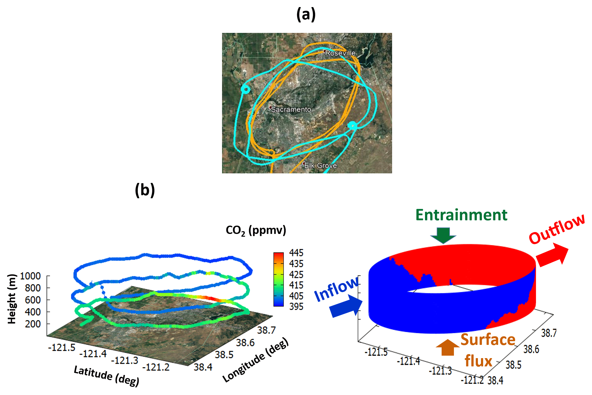
Figure 1(a) Map of AJAX flight tracks on 18 November 2013 (orange) and 29 July 2015 (cyan) plotted in Google™ Earth. (b) Vertical measurements of CO2 mixing ratio on 18 November 2013, and (c) simple illustration of airflow (kg m) passing through the cylinder (over Sacramento). The color represents the air mass flux (density, kg m−3; multiplied by wind vector, m s−1) normal to the cylinder. The blue and red represent inflow and outflow, respectively. The vertical mass transfer through the top and bottom are referred to as the entrainment and surface flux, respectively.
One approach for estimating CO2 and CH4 fluxes over cities is the use of an aircraft-based mass balance method. Several studies have demonstrated the utility of this approach (Kalthoff et al., 2002; Mays et al., 2009; Turnbull et al., 2011; Karion et al., 2013, 2015; Cambaliza et al., 2014; Gordon et al., 2015; Tadić et al., 2017). Mass balance methods utilize many length scales and patterns. The flights target mostly local scales (< 3 km) and areas around point sources (Nathan et al., 2015; Conley et al., 2017), but they also characterize urban scales (e.g., 25×10 km for Gordon et al., 2015, 4×9 km for Tadić et al., 2017) and larger scales (40 km up to 175 km, especially for a downwind curtain flight; Mays et al., 2009; Turnbull et al., 2011; Karion et al., 2015).
The flight patterns can be classified into three different categories: (1) single-height transect flight, (2) single screen (“curtain”) flight with multiple transects, and (3) enclosed shapes (box, cylinder) (see Fig. S1 in the Supplement). Commonly, there are assumptions made in these airborne sampling approaches. First, the single-height transect approach assumes a well-mixed boundary layer. Karion et al. (2013) measured CO2 and CH4 along a single-height transect with an assumption of uniform distribution of trace gases with altitude within the planetary boundary layer (PBL) and with time. Turnbull et al. (2011) performed a flux estimate by incorporating detailed meteorological information and transecting an emission plume with an aircraft. These studies also assumed that emissions originate from point sources such as pipes and smokestacks, and travel downwind so that all pollution is reflected on the downwind curtain with constant wind speed. Second, the single-screen multi-transect method does not assume a uniformly mixed boundary layer condition but is dependent upon constant wind speed. Without a well-mixed boundary layer assumption, Cambaliza et al. (2014) measured CH4 along multiple height transects downwind of the city of Indianapolis (see Fig. S1a in the Supplement). However, they assumed that winds at the time of measurement were the same as at the time of emission (i.e., winds after the methane release were time-invariant). Third, the enclosed 3-D shape flights do not presuppose any of the assumptions described above. Gordon et al. (2015) measured various GHGs with a stacked box flight pattern, to capture the vertical variation in mixing ratio both upwind and downwind. Tadić et al. (2017) and Conley et al. (2017) accomplished emission estimates by flying a cylinder pattern around an emission source to measure GHGs both upwind and downwind for analysis based on the divergence theorem. More recently, Baray et al. (2018) used both a screen flight and box flight approach around oil sands facilities and showed that each flight pattern could be preferred, depending on the types of emissions and spatial characteristics.
The method of extrapolation to unsampled areas can also be a large source of uncertainty. For example, Gordon et al. (2015) demonstrated the significant impact of extrapolation methods over the unsampled, near-surface region on the final emission estimate, unlike Cambaliza et al. (2014), who assumed that the city plume is rarely observed in a transect between the surface and the lowest-altitude flight measurement. Assumptions can break down when wind direction and speed vary with time and three-dimensional space (see Fig. S1); incorrect use of wind data can result in increased uncertainty and reduction of accuracy. Flux estimates also require an estimate of the planetary boundary layer height (PBLH), an important physical parameter. State-of-the-art atmospheric models and reanalysis products often estimate the PBLH, but substantial differences exist in both models and reanalysis data (Wang and Wang, 2014). In addition, entrainment from the free troposphere into the planetary boundary layer (PBL) and fluxes from the surface have been ignored in most previous studies. Thus, more careful consideration and understanding of these factors are required for determining emission estimates using any of the three mass balance flight patterns.
The primary goals of this study are (i) to assess the impact of different interpolation and extrapolation methods on the emission estimate, (ii) to test the sensitivity of emission estimates to a variety of factors such as wind treatment, background mixing ratios, and different flux estimation methods, and finally (iii) to examine the importance of vertical mass transfer on the flux estimates. To address these goals, we present here CO2 and CH4 data collected during two research flights over Sacramento (see Figs. 1a and S2 in the Supplement) for urban (25–40 km) and local scales (< 3 km), and determine emission fluxes using various treatments of wind conditions, background mixing ratios, and vertical mass transfer. The data and methodology are presented in Sect. 2. Calculated CO2 and CH4 fluxes for all flights are shown in Sect. 3. The sensitivities of flux estimates to different treatment of the wind, background, and vertical mass transfer are also investigated. The conclusions of this study are presented in Sect. 4.
2.1 Data collection
In situ measurements of CO2 and CH4 were performed as part of the Alpha Jet Atmospheric eXperiment (AJAX) project. As can be seen in Fig. 1, flights were generally performed in large, nominally oval circuits around the Sacramento urban area. The shape and size of the circuits depended on air traffic control considerations on an individual flight day, with the goal of circumscribing an area of approximately 25 km × 40 km. Level circuits at multiple altitudes at and below the top of the boundary layer were performed. In addition to the regular urban-scale flight pattern, this paper also presents data from a flight designed to study two local-scale features enclosed by the small circles in the cyan flight track shown in Fig. 1a. Sampling occurred at 21:10–22:00 UTC on 18 November 2013 (local standard time is UTC minus 8 h, 13:10–14:00 PST) and 20:55–21:45 UTC on 29 July 2015.
The CO2 and CH4 instrument (Picarro Inc., model 2301-m) is calibrated before each flight using two whole-air standards from the National Oceanic and Atmospheric Administration's Earth System Research Laboratory (NOAA/ESRL; CO2=416.267 and 393.319 ppmv; CH4=1.98569 and 1.84362 ppmv). In addition, a set of secondary, synthetic standards was used to verify the linearity of the instrument across a wider range of concentrations. Water vapor corrections using Chen et al. (2010) were applied to calculate the dry mixing ratios of CO2 used during this study. The overall uncertainty was determined to be 0.16 ppm for CO2 and 2.2 ppb for CH4 (Tanaka et al., 2016; Tadić et al., 2014). The Meteorological Measurement System (MMS) measures high-resolution pressure, temperature, and 3-D (u, v, and w) winds (Hamill et al., 2016). The CO2 and CH4 mixing ratios and horizontal wind speed are plotted in Fig. 2.
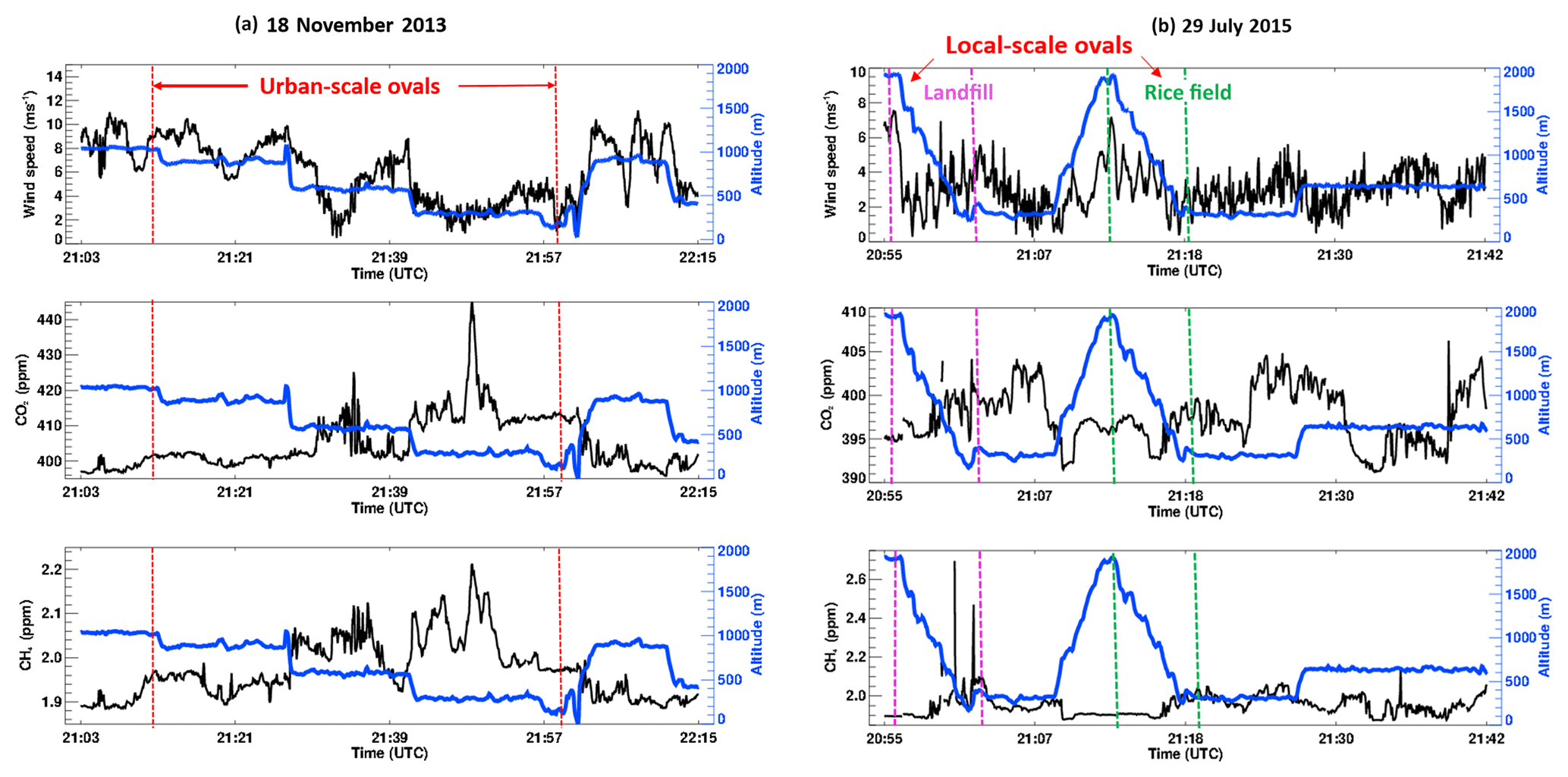
Figure 2(a) A time series of (black lines) CO2, CH4, horizontal wind speed, and (blue lines) altitude of the aircraft for 18 November 2013. The red dashed lines represent the portion of the flight over Sacramento. (b) The same as Fig. 2a except for 29 July 2015. The magenta dashed lines indicate the portion of the flight over the landfill, and the green dashed lines mark the start and end times of the rice field measurements.
2.2 Data gridding
2.2.1 Extrapolation to the surface
Because the lowest flight level was typically between 250 and 380 m above the surface and there were no ground-based measurements along the flight tracks, there is always a gap in measurement data between the surface and the lowest flight altitude. Many studies adopt a well-mixed layer assumption below the lowest flight altitude (Karion et al., 2013), but the unmeasured values can lead to a significant bias and large uncertainties in estimating GHG mixing ratios and fluxes, depending on interpolation and extrapolation schemes, especially at lower altitudes where there are no aircraft data available (Gordon et al., 2015). Thus, here we investigated four methods to extrapolate mixing ratio values to the surface, which are termed (1) constant, (2) exponential, (3) Gaussian, and (4) kriged (see Fig. 3). The constant method assumes an elevated plume with a constant mixing ratio. The constant mixing ratio here is derived from the lowest flight measurement: for , where zL is the lowest flight level. The exponential-fit method assumes an exponential increase in X(t,z) from zL to z0. The Gaussian fit method is similar to the exponential fit method, except that the surface-sourced plume dispersion follows a Gaussian distribution function. The detailed calculation method is based on Gordon et al. (2015). The kriged fit was applied down to the surface level, extended from the sampled area above.
Figure 3a and 3b show observed and estimated CO2 mixing ratios at several locations over Sacramento on 18 November 2013. These results demonstrate that a large source of uncertainty and difference comes from not only the interpolation between flight levels but also the extrapolation of the data between the lowest flight level and the surface. For example, uncertainty in estimated GHG mixing ratios below the lowest flight level (indicated by the yellow diamond) can be large (up to ∼20 %). In the worst cases, CO2 mixing ratios span more than 80 ppm at the surface among the methods (Fig. 3b); CH4 ranges > 0.15 ppm. Note that the differences between interpolation schemes where data exist (above ∼250–380 m) are smaller than the differences between various methods below the lowest flight data. Without ground-based data, a proper choice of extrapolation schemes requires knowledge or presumption of the mixing ratio behavior in this region. Gordon et al. (2015) proposed that the case of elevated sources beneath the lowest flight level is best suited to constant extrapolation of mixing ratio to the surface (blue curve), while a ground source should be represented with an exponential-fit extrapolation (red).
The various fits rely on different assumptions; the ordinary kriging method (magenta trace in Fig. 3b) also requires some assumptions (e.g., constant mean, constant variance, second-order stationarity and isotropy, and validity of the theoretical model), but the method leverages spatial and statistical properties of the observations to derive estimates, and seems to be less arbitrary than alternative interpolation–extrapolation methods. We note the similarity between the kriged values and the constant extrapolation method for both CO2 and CH4 (not shown). The Gaussian and the exponential extrapolations produce large values below the measurement level, increasing the uncertainty. However, the values above the lowest measurement level are very similar among the different fit methods. This indicates how sensitive the final flux estimate can be depending on the given interpolation and extrapolation method and how much care should be taken when selecting the extrapolation methods when no data are available.
2.2.2 Elliptical fit and measurement interpolation (Kriging method)
Because the aircraft flew in a cylindrical pattern around the city, the flight paths were transformed into a polar coordinate system. The path was projected to the surface first and fit into an ellipse using the least-squares method to minimize the difference between the measured data and the fitted data. Then, we computed each point using the major and minor axes of the ellipse and parameter t. Each point on the ellipse was represented by a single parameter (t, eccentric anomaly), according to the following equations:
where a and b are the radius of the major and minor axes of the ellipse, φ is the angle between the X axis and the major axis of the ellipse, and the parameter t is obtained from Eq. (1), varying from 0 to 2π. Then, the data were gridded into a two-dimensional plane (t, height).
In order to assess the strengths of a kriging approach to quantifying emissions, two interpolation methods were assessed: interpolation using kriging and interpolation using an exponential weighting function (see Fig. S3). The exponential weighting function at a given point (P) was defined as the weighted average of all the other points where the weights decrease exponentially with distance to P. Both approaches captured the general plume pattern (regions with high and low concentrations of CO2), but the kriging approach did better at capturing individual plume features such as the range and magnitude, while interpolation with the exponential weighting function could not resolve such details. Another benefit of kriging is that it can estimate values at unsampled locations using a weighted average of neighboring samples, thus reproducing the characteristics of the observed values.
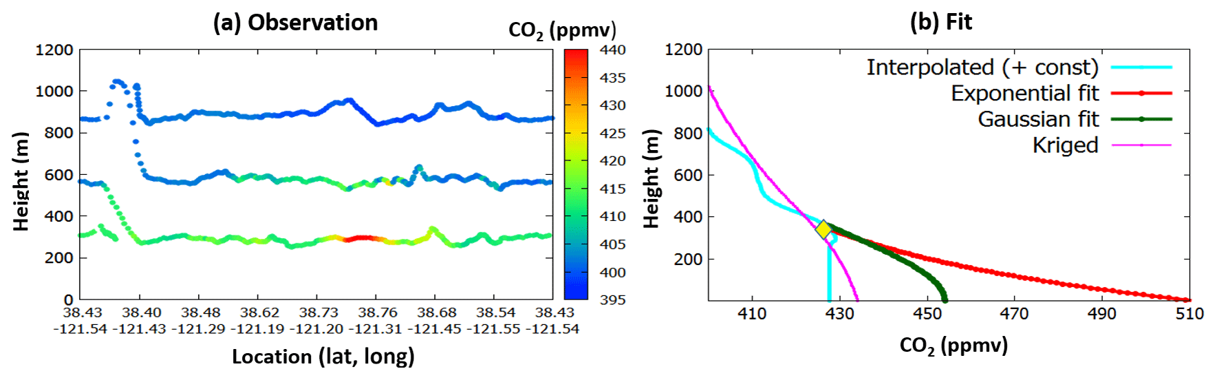
Figure 3(a) Observed CO2 over the Sacramento loop on 18 November 2013. (b) The vertical profiles of calculated CO2 mixing ratios around 38.75∘ N, 121.27∘ W. The yellow diamond indicates the altitude of the lowest flight data. The kriged values (magenta), interpolated values with exponential weighting function, and extrapolated values using constant (cyan), Gaussian fit (green), and exponential fit (red) are compared. The empirical fits were generated based on the approach by Gordon et al. (2015).
Interpolation was performed by the ordinary kriging method (Chilés and Delfiner, 2012), modified from the IDL v8.1 kriging tool to fit an elliptical pattern. We chose ordinary kriging because there is no obvious trend in the data we use. Before kriging, we modeled the variograms for all relevant variables. A variogram (or semivariogram) is a function describing the degree to which the data are correlated as a function of the separation distance between observations. The empirical semivariogram of the data was fit using an exponential variogram model, based upon visual inspection of the experimental variograms. Three parameters were used to fit the theoretical variogram, namely the sill (the expected value of the semivariance between two observations as the lag distance goes to infinity), the range (the distance at which the variogram reaches approximately 95 % of the sill), and the nugget (representative of measurement error and amount of microscale variability in the data). Variogram modeling was first performed to derive parameters required to obtain ordinary kriged estimates. Various other types of kriging exist in the literature on quantifying greenhouse fluxes (Tadić et al., 2017), but examining their differences is beyond the scope of this study.
We kriged the CO2, CH4, wind, temperature, and pressure observations to obtain both the estimate and the uncertainty for each variable at each grid point. The individual semivariograms of the variables for each flight were produced, and we present them for one flight in Fig. S4 in the Supplement. For each flight, the sampled data were kriged to a grid of maximum height divided by 150 in the vertical dimension; the horizontal dimension was kriged from end to end of the flight transect, enclosing the circumference of the entire city, divided by 360 in the horizontal direction. The vertical dimension was interpolated from the ground to the top of the flight measurement, but only data up to the estimated planetary boundary layer height (PBLH) were used for computing the flux estimates.
Figure 1 shows a map of the AJAX flight tracks on 18 November 2013 and 29 July 2015 over Sacramento and the vertical structure of the CO2 mixing ratio on 18 November 2013. A simple illustration of the air flow demonstrates the basic idea of this study, Gauss's divergence theorem, which relates the flow through the surface to the volume of the cylinder (Fig. 1c). Mass coming in and out of the cylinder should be conserved if there is no leak through the top or the bottom of the cylinder (i.e., the flow into the cylinder balances with the flow out of the cylinder). More precisely, the surface integral through a closed system is equal to the volume integral of the divergence over the region inside the surface. Since the atmosphere has no upper boundary, we assume that vertical mass transfer is accomplished through entrainment from the top of the PBL and surface flux from the bottom of the cylinder near the surface. In this way, the oval cylinder we design over the city has a closed surface, and the flux inside the cylinder is equal to the sum of the emission flux at the bottom.
In Sect. 3.1 we will first describe the “base case” calculation of fluxes, and in Sect. 3.2 we report the sensitivity of the fluxes to variations in several aspects of the method.
3.1 Base case experiment
Our base case experiment used the entire gridded, enclosed elliptical data curtain using kriging as both the interpolation and extrapolation method. We averaged the measured wind in vertical layers 100 m thick so that air (mass) coming into the cylinder equaled air leaving the cylinder (which we refer to as “mass-balanced wind”). We assigned the background to be the minimum concentration found in each 100 m layer. PBLH was determined as the altitude of the maximum gradient from a vertical profile of potential temperature (Wang et al., 2008) obtained from the MMS measurements during each flight. We included entrainment from the top and surface flux from the surface. The results of this base case are displayed in the top rows of Tables 1 (urban scale) and 2 (local scale).
Here we define the entrainment (surface) flux as the turbulent flux of the scalar at the boundary layer height (surface) (Faloona et al., 2005). Then we compute the entrainment flux at the top of the cylinder by multiplying the area of the top of the cylinder with , where A is the area of the top of the cylinder, is the CO2 (or CH4) mass concentration (g m−3) converted from the CO2 (or CH4) mixing ratio (ppmv) at a given point, t, along the perimeter of the top of the cylinder at z=h, and Cbg(h) is the background concentration of CO2 (or CH4) at the top of the boundary layer. The CO2 (CH4) mass is calculated from the CO2 (CH4) mixing ratio (ppmv). Using this, we could make direct observations of the entrainment flux by measuring vertical velocity together with the trace gas mixing ratio throughout the boundary layer. The surface flux is computed at the surface (z=0) in a similar manner.
We determined kriged data for each field from the measured CO2, CH4, wind, temperature, and pressure, and then subtracted background values from the trace gas data at each grid point. To convert the volume mixing ratio (ppmv) to a mass concentration (g m−3), the number of CO2 or CH4 molecules were computed based on the ideal gas law using the kriged temperature and pressure. Then, the net mass flow (g m−2 s−1) was integrated in the horizontal and vertical directions from the surface up to the top of the cylinder.
where L is the difference between two points on the ellipse, is the wind speed, α is the angle of the wind velocity relative to the flux surface, C is the concentration (g m−3), and Cbg is the background concentration at each level z. The component of the wind perpendicular to the flux surface was used in the flux calculation.
Figure 4 shows the measured methane over Sacramento, CA, for 18 November 2013, the projection to the ground, and the computed “flux surface”. The kriged CH4 not only captures the measured CH4 mixing ratio but also fills the unsampled area based on the observed data characteristics. Maximum values were found at 38.73∘ N, 121.2∘ W to 38.68∘ N, 121.45∘ W at 300 m. The high CH4 region corresponds with highways, landfills, and dairy farms.

Figure 4(a) Map of AJAX flight tracks colored by CH4 mixing ratio for 18 November 2013, plotted in Google™ Earth. (b) The data (red) fitted to an oval (green). The observed CH4 mixing ratios (c) are kriged to generate the cylindrical surface (d). The axes of the oval are approximately 25 and 40 km. The yellow arrow represents the dominant wind direction.
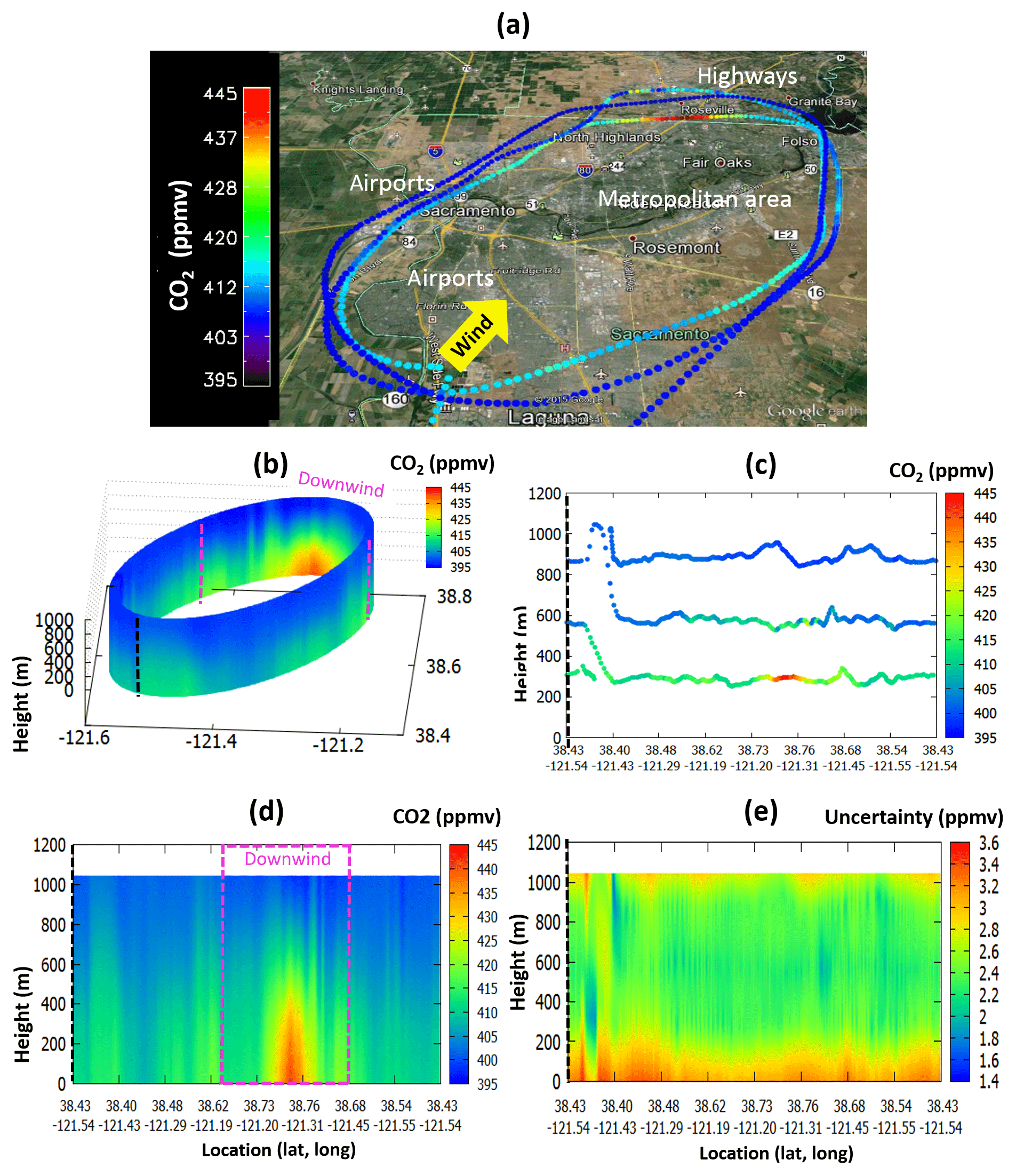
Figure 5(a) A map of AJAX flight track overlaid by the CO2 mixing ratio, plotted in Google™ Earth, (b) kriged CO2 mixing ratio, (c) measured CO2 mixing ratio, (d) the same as (b) except plotted in two dimensions, and (e) kriging uncertainty at each grid point on 18 November 2013. The yellow arrow represents the dominant wind direction, and the black dashed line indicates where the surface is split open. The area enclosed by the magenta dashed lines represents the area we used as a downwind portion. Figures are stretched vertically by about a factor of 100.
For the same flight, Fig. 5 shows the observed and kriged CO2 mixing ratio and kriging uncertainty at each grid point. The kriged CO2 field captures the main features of the observed CO2 plume well. The CO2 mixing ratios were much larger (up to 25 ppm higher at most spots) on the downwind side than the upwind side. The observations in Fig. 5b–e suggest that the vast majority of the emissions sampled by the flights originates in the region identified as traffic regions (Roseville), airports, and metropolitan areas (Arden-Arcade, Roseville, North Highlands, Fair Oaks) (see the map in Fig. 5a). Uncertainties of CO2 were large near the surface, small from 200 to 900 m, and grew larger near the top of the sampled domain.
The vertical stretching pattern of CO2 mixing ratios in Fig. 5d and e appears to be due to the large-scale difference between the horizontal length (> 120 km) and the vertical length (< 1 km). When we applied our method to the local scale (horizontal scale < 3 km; see Fig. 7), or took a small horizontal portion of the large oval (see Fig. S3 in the Supplement), the vertical stretching pattern disappeared.
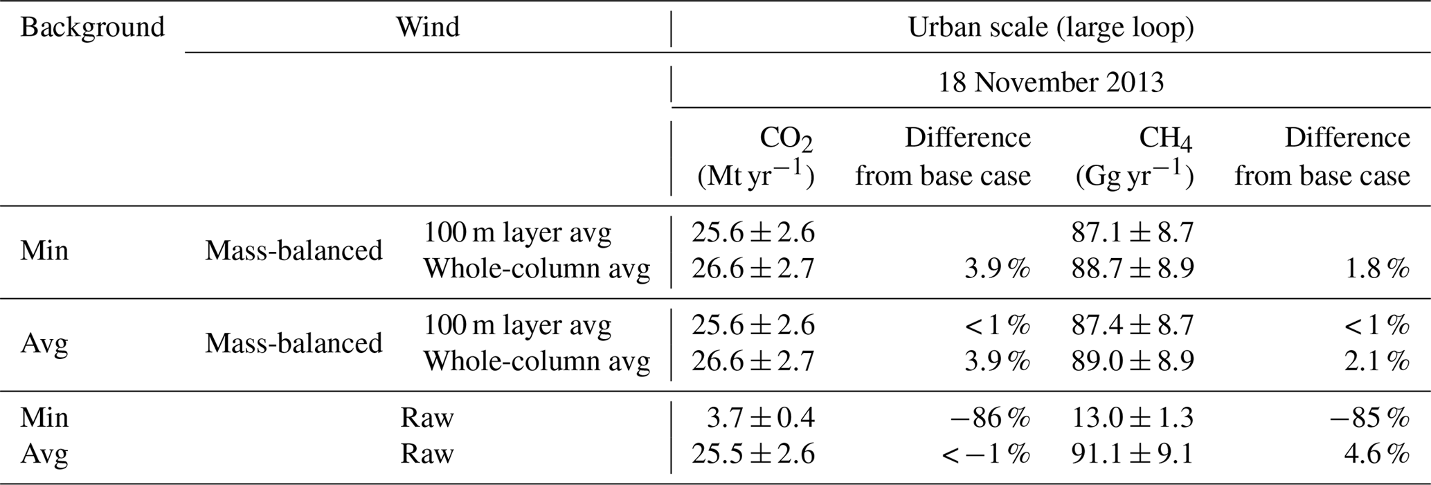
As shown in the top row of Table 1, we determined urban-scale flux values of 25.6±2.6 Mt CO2 yr−1 and 87.1±8.7 Gg CH4 yr−1 for this base case experiment. Note that we do not consider the uptake of CO2 by vegetation, but the biological impact on CO2 flux will be important, especially during summer.
Table 1Urban-scale CO2 and CH4 fluxes over Sacramento using different wind treatment (raw wind: “raw”, or mass-balanced wind: “mass-balanced”) and different background values (minimum or average values) on 18 November 2013. The vertical mass transfer (entrainment and surface flux) is included in these calculations. “Whole-column avg” means the vertical column average up to the estimated PBLH.
3.2 Sensitivity tests
3.2.1 Sensitivity of calculated flux to interpolation–extrapolation method
As shown in Fig. 3b, there is a large source of uncertainty and difference due to extrapolation of the data between the lowest flight level and the surface. For example, CO2 mixing ratios span more than ∼80 ppm near the surface among the methods (∼20 %); CH4 ranges > 0.15 ppm (∼8 %). This implies that a proper choice of extrapolation scheme requires knowledge or presumption of the mixing ratio behavior in this region when there are no ground-based data. Gordon et al. (2015) proposed that the case of elevated sources beneath the lowest flight level is best suited to constant extrapolation of mixing ratio to the surface (cyan curve), while a ground source should be represented with an exponential-fit extrapolation (red). Note that the differences of the mixing ratio between interpolation schemes where data exist (above ∼250–380 m) are smaller than the differences of the mixing ratio between various methods below the lowest flight data for both CO2 and CH4.
While it is important to make the best possible choice among different GHG mixing ratio extrapolations, similar uncertainty in how best to treat the wind below the lowest flight level makes calculations propagating the effect of each extrapolation scheme challenging, and exploration of the isolated impact of the extrapolation of GHG mixing ratios is of limited value. In general terms, and making reasonable assumptions for the estimation of wind, boundary layer height, and background, we expect the sensitivity of calculated flux to the interpolation method is small above the lowest flight level, but the sensitivity of calculated flux to the extrapolation method below the lowest flight level will be more than 20 % depending on the usage of wind, leading to difference in the final flux estimate.
3.2.2 Sensitivity of calculated flux to wind treatment
Wind variability and measurement assumptions can lead to errors in the CO2 and CH4 flux estimates (Mays et al., 2009; Cambaliza et al., 2014, 2015; Nathan et al., 2015; Karion et al., 2013, 2015), and the way in which winds are estimated and quantified in particular matters. To test the sensitivity of fluxes to the treatment of wind, we applied the measured high-resolution (1 Hz) in situ wind data to the flux calculation in two different ways. We averaged horizontal wind on each vertical level (100 m for the base case, 500 m (not shown), or the whole cylinder as one layer), so that air (mass) coming into the cylinder equaled air leaving the cylinder. We also evaluated the calculated fluxes when the measured wind was used without any averaging (hereafter we refer to it as “raw wind”). In this case, inflow and outflow are not required to be balanced.
For 18 November 2013, the wind was southwesterly at the low altitudes, but it changed its direction to southeasterly as height increased. Figure 6 demonstrates the clear difference in flux estimates when the 2-D raw wind or the mass-balanced wind is used. The right column in Fig. 6 shows that we captured high fluxes when we used the mass-balanced wind (panels b and c), while we were less likely to obtain a strong emission signal when using the raw wind data (panel a), which might be attributed to an imbalance of inflow and outflow to the cylinder. The total flux difference was ∼7 times higher or lower between wind cases: 3.7 Mt CO2 yr−1 and 13.0 Gg CH4 yr−1 calculated with raw wind, and 25.6 Mt CO2 yr−1 and 87.1 Gg CH4 yr−1 using mass-balanced wind with a 100 m vertical average, leading to 86 % and 85 % difference compared to the base case (see Table 1).
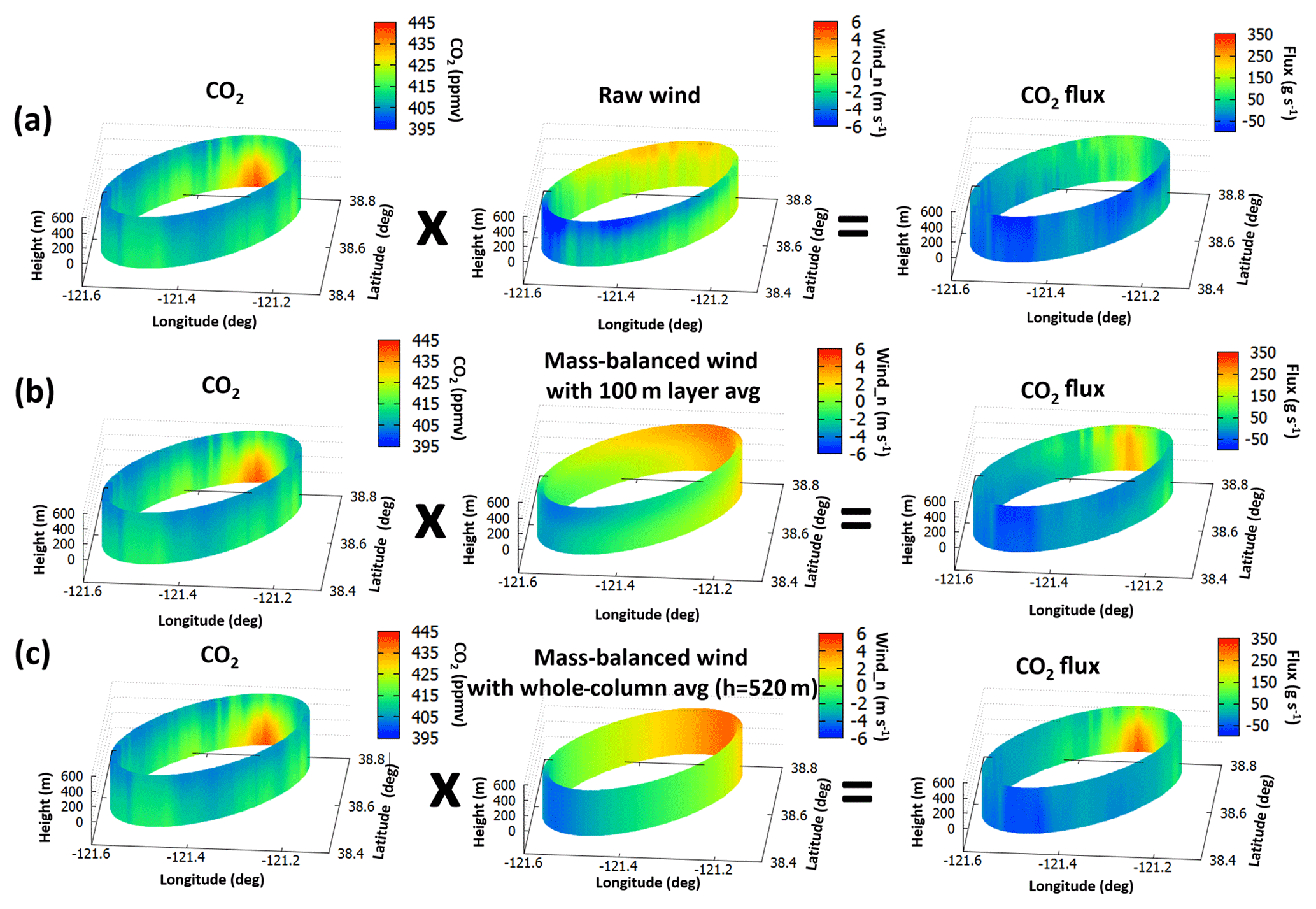
Figure 6(a) Kriged CO2 mixing ratio, the raw wind, and CO2 flux using the raw wind; (b) kriged CO2 mixing ratio, 100 m vertically averaged mass-balanced wind, and CO2 flux using the mass-balanced wind; and (c) kriged CO2 mixing ratio, the whole-column-averaged mass-balanced wind, and CO2 flux using the mass-balanced wind on 18 November 2013. In the middle column, the blue color represents the inflow toward (and red outflow from) the cylinder so that it is defined as negative (positive) wind. The background CO2 was chosen as the minimum mixing ratio at each vertical layer. The whole-column average means the vertical average from the surface to the top of the planetary boundary layer height (PBLH). Figures are only shown below the PBLH.
The importance of wind data on the flux calculation is also seen in local-scale emission calculations, but not as dramatically as in those for the urban scale (see Table 2). For the small cylinder over the landfill site on 29 July 2015, Fig. 7 shows the observed and kriged CH4 mixing ratio and the flux estimation using the raw wind and mass-balanced wind over the landfill site. As before, the kriged CH4 is a good representation of the local characteristics of the CH4 field. Reassuringly, the elevated CH4 concentration was reconstructed over 121.19∘ W, 38.52∘ N, which was close to the nearby landfill (see also Figs. 4 and S6 in the Supplement). Considering light wind conditions (< 4 m s−1) and high temperature during July, the high flux estimates are attributed to the local emissions. For the local scale, the difference in the flux estimate using the raw wind and mass-balanced wind is relatively small. For example, even when using raw wind over the landfill, the difference of the calculated flux from the base case is ∼25 % for CH4, which is about one-third smaller than the difference of calculated flux from the base case for the urban scale (∼85 %) for CH4. For CO2, when using raw wind the difference of calculated flux from the base case becomes larger, but it is still smaller than the difference for the urban scale (see Table 1).
Table 2Local-scale CO2 and CH4 fluxes over landfill and rice field locations in Sacramento using different wind treatment (raw wind: “raw”, or mass-balanced wind: “mass-balanced”) and different background values (minimum or average values at each level) on 29 July 2015. The vertical mass transfer (entrainment and surface flux) is taken into account. “Whole-column avg” means the vertical column average up to the estimated PBLH.
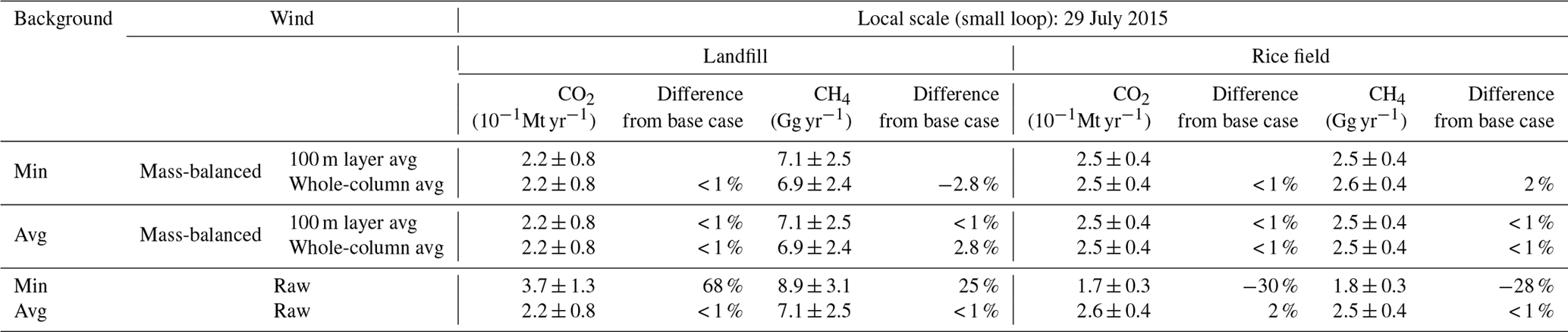
Another interesting finding here is the importance of the vertical averaging effect of wind, which is also shown in Figs. 6 and 7. Even when using the mass-balanced wind, the whole-column-averaged wind can underestimate or overestimate the final flux estimate depending on the situation. Certainly, care needs to be paid when treating wind as a mean in both the horizontal and the vertical. Many previous studies estimated CO2 and CH4 fluxes based on the mean wind vector at the dominant wind direction (positive and one direction) and speed (Turnbull et al., 2011; Karion et al., 2015), often using simulated wind obtained from a coarse-resolution model. Even when using high-resolution measured winds in place of coarse-resolution model data, we can see the impact of averaging wind on the flux estimate. However, overall, the choice of raw wind or mass-balanced wind is more important than the thickness of the vertical averaging for mass-balanced wind for flux estimate for both urban and local scales. Furthermore, the flux estimates using raw wind are more sensitive to the choice of the background for both urban and local scales. For example, when we use raw wind with average background concentration, the flux estimate is about the same as the base case flux estimate (see bottom rows in Tables 1 and 2).
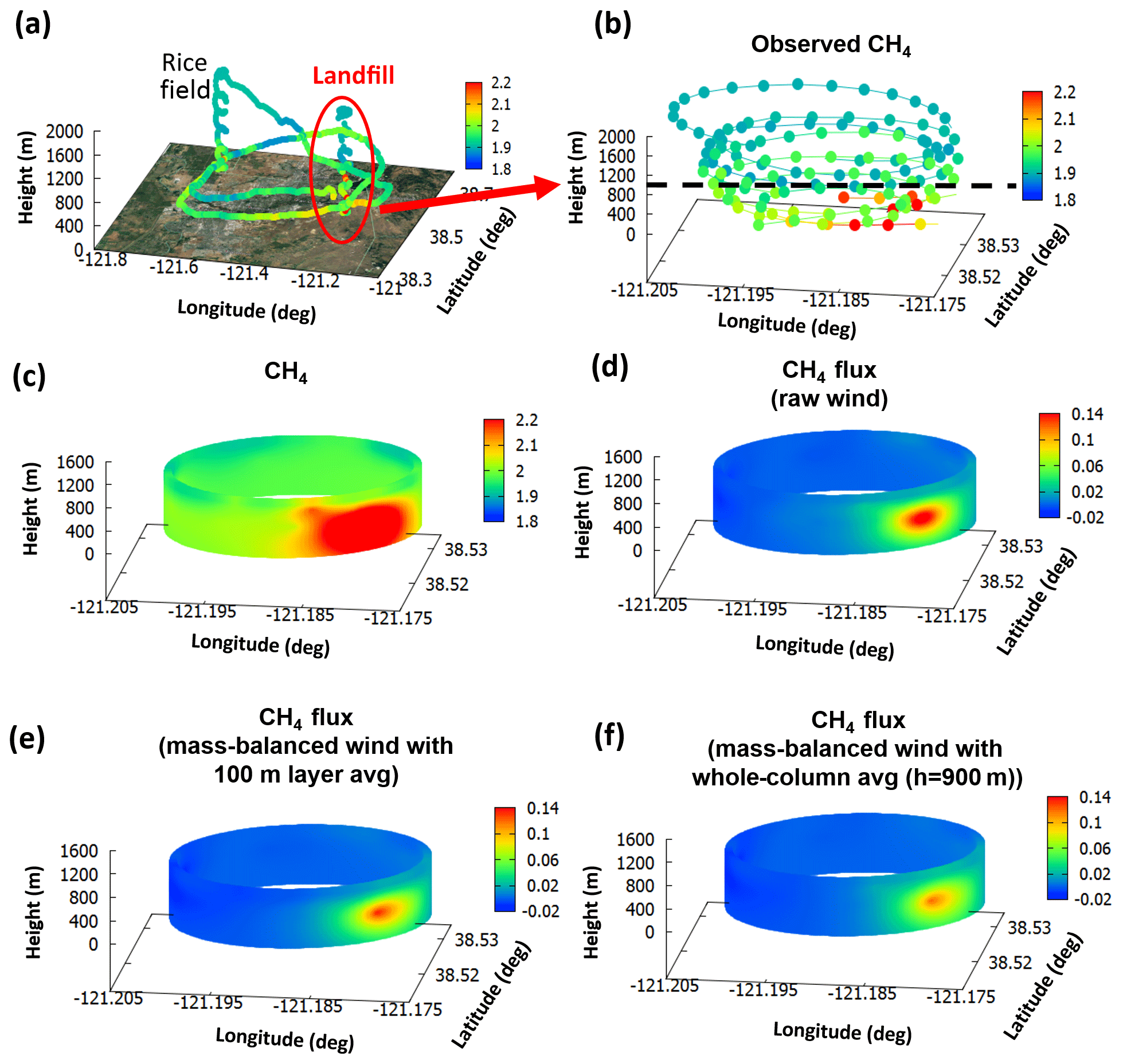
Figure 7(a) The map of AJAX flight track with the observed CH4 mixing ratio. (b) The observed CH4 mixing ratio, (c) kriged CH4 mixing ratio, (d) CH4 flux using raw wind, (e) CH4 flux using the mass-balanced wind with 100 m vertically averaged wind, and (f) CH4 flux using mass-balanced wind (averaged through the entire PBLH) over the landfill location on 29 July 2015. The fluxes are computed based on Eq. (2). The background value was chosen as the minimum value at each vertical layer. The approximate diameter of the cylinder is 3 km, and the color scale is capped at 2.2 ppmv in panels (a)–(c). The black dashed line represents the top of the PBLH for this flight. Panels (c)–(f) are only shown below the PBLH.
3.2.3 Sensitivity of calculated flux to the choice of background concentrations
Background values are one of the most important factors in obtaining flux estimates, and theoretically, the background values should be canceled out for the enclosed-shape mass-balance flight. Here we used several distinct methods to determine background values and calculate emission fluxes for each gas to assess if our method could remove some of the uncertainty due to assigning the background. As in the base case, we used the minimum concentration over the layer height (e.g., 100 m or whole-column averaging). In comparison, we also calculated fluxes using the average concentration in each layer as the background. Third, we also tested two different, vertically invariant, constant values.
Tables 1 and 2 show the calculated CO2 and CH4 emission fluxes using two different wind methods and two different background treatments. The rows labeled “min” were generated using the minimum kriged mixing ratio in each altitude band as the background for all data at that level. The rows identified by “avg” used the average mixing ratio in each altitude band as the background on that level.
The bottom two rows of Tables 1 and 2 show the sensitivity of calculated flux to the choice of the background treatment was significant when we used raw wind; the estimate using average concentration for the background closely matched the base case, but using the minimum concentration for the background resulted in significantly different calculated fluxes, as we mentioned earlier. This was true both with the vertical mass transfer (Table 1) and without (not shown). In contrast, when we use the mass-balanced wind, the emission estimates for both CO2 and CH4 are nearly identical for either choice of background treatment. Interestingly, when an average mixing ratio at a given vertical level is used for the background concentration, emission estimates with raw wind are similar to emission estimates with mass-balanced wind. To satisfy mass conservation, we also computed the entrainment flux from the top (z=h) and the surface flux from the bottom of the cylinder (z=0). The data from Table 1 are also shown in Fig. 8 as the non-hatched bars.
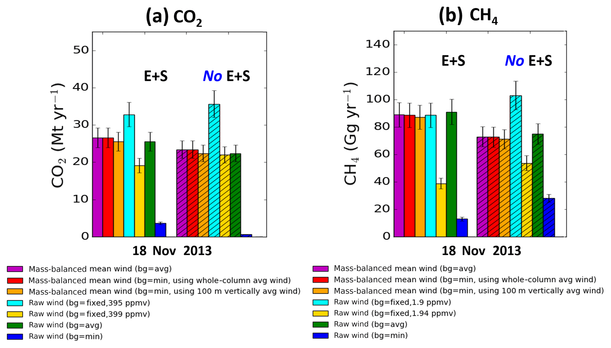
Figure 8Urban-scale (a) CO2 (Mt yr−1) and (b) CH4 (Gg yr−1) emission rate estimates using raw wind and mass-balanced wind, with different background treatments. Solid bars represent emission estimates including entrainment and surface flux (E+S), and hatched bars represent the corresponding emission estimates without consideration of entrainment and surface flux (No E+S). Error bars represent the uncertainty of the total emission fluxes. The average and minimum values for the background were computed at each vertical layer (100 m or whole-column average), and the fixed value alternatives were 395 or 399 ppm for CO2 and 1.90 or 1.94 ppm for CH4 for all altitudes.
3.2.4 Sensitivity of calculated flux to vertical mass transfer
Many previous studies assume that vertical mass transfer can be neglected (Cambaliza et al., 2014; Conley et al., 2017). To quantify the validity of this assumption, we compare in Fig. 8 the flux determined when including or neglecting the entrainment and surface fluxes. Multiple implementations were tested, as shown in different colors. The differences between CO2 and CH4 fluxes calculated with (left side of each panel) and without (right side, hatched bars) vertical mass transfer were determined to be about 11 % for CO2 and 21 % for CH4 on the urban scale and less important for the local emission estimates (< 8 %, not shown).
3.2.5 Sensitivity of calculated flux to the PBLH estimate
We also considered the sensitivity of the calculated flux to the PBLH. The potential temperature profile, which indicates atmospheric static stability and which significantly affects pollutant diffusion, is one of the most common operational methods to determine PBLH. No significant sensitivity was found using several different PBLH detection algorithms, such as the parcel method (the interaction between dry adiabatic lapse rate and temperature), rapid decrease in water vapor (Wang and Wang, 2014), or Richardson number method (Wang et al., 2008). A simple example is shown in the Supplement Fig. S5. When we determined the PBLH based on the largest gradient of the vertical profile of the potential temperature, the uncertainty due to PBLH estimate for the urban scale is about ∼10 %, and that for the local scale is about 1 %–5 %; thus the change in PBLH does not affect the total flux estimate, especially for the local scale. As seen in Fig. S5, the vertical range of the largest gradient of potential temperature is very small for the local scale, compared to the urban scale. This leads us to another important message: the uncertainty can increase when we consider urban-scale flux estimates.
3.2.6 Sensitivity of calculated flux to the closed shape
Our citywide estimate of about 25.6±2.6 Mt CO2 yr−1 (e.g., using the base case of mass-balanced wind with minimum background concentration) is higher than the result by Turnbull et al. (2011), who reported 13.4 Mt CO2 yr−1 (3.5 MtC yr−1) over Sacramento in February 2009 (see Table 3). But if we examine only the small downwind portion of the ellipse which shows the highest CO2 mixing ratio (e.g., 121.45–121.20∘ W and 38.65–38.76∘ N in 2013; see Fig. 5b and d), CO2 fluxes calculated using mass-balanced wind with minimum concentration for the background were about 17.3±1.7 Mt yr−1 in 2013, in much better agreement with Turnbull et al. (2011). When calculating fluxes using mass-balanced wind with average concentration for background, the “downwind side” emission estimates were 8.9±0.9 Mt CO2 yr−1. According to these calculations, the fluxes from the downwind portion of the cylinder were responsible for only ∼35 %–68 % of the total emissions. The Turnbull et al. (2011) data were collected in 2009; the value given here was converted from the mean reported value of 3.5 Mt C yr−1 with a 1.1 % yr−1 increase in CO2 flux to adjust to 2013 (Turnbull et al., 2011). Bottom-up inventory estimates of the annual total emissions from Sacramento County from Vulcan (Gurney et al., 2009) and the California Air Resources Board CEPAM database (Turnbull et al., 2011) are included for comparison for CO2. The Vulcan inventory is available only for 2002, and the CEPAM database is available for 2004. We applied a 1.1 % yr−1 increase in CO2 flux to adjust to 2013.
Table 3Flux estimates for the Sacramento urban area from measurements made on 18 November 2013. The two “curtain” calculations used the same wind treatments as the “whole cylinder” calculations (mass-balanced wind). Turnbull et al. (2011) data were collected in 2009; the value given here was converted from the mean reported value of 3.5 Mt C yr−1 with a 1.1 % yr−1 increase in CO2 flux to adjust to 2013. Bottom-up inventory estimates of the annual total emissions from Sacramento County from Vulcan (Gurney et al., 2009) and the California Air Resources Board CEPAM database (Turnbull et al., 2011) are included for comparison for CO2. The Vulcan inventory is available only for 2002, and the CEPAM database is available for 2004. We applied a 1.1 % yr−1 increase in CO2 flux to adjust to 2013. The gridded (0.1∘ × 0.1∘) National U.S. Environmental Protection Agency (EPA) Inventory for November 2012 is included for comparison for CH4. We applied a 0.6 % yr−1 increase in CH4 flux to adjust to 2013.
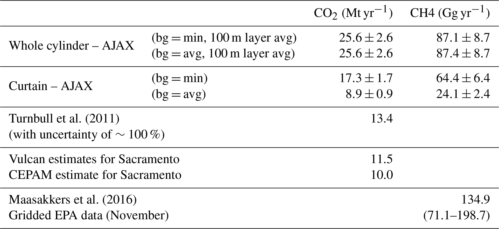
Our citywide estimate of 87.1 Gg CH4 yr−1 (e.g., flux estimate using 100 m vertically averaged mass-balanced wind) on 18 November 2013 corresponds to 52 % of the 167 Gg CH4 yr−1 (∼140–220 Gg yr−1) reported by Jeong et al. (2016) over Region 3 (Sacramento Valley) for 2013–2014. The Gridded (0.1∘ × 0.1∘) 2012 National U.S. Environmental Protection Agency (EPA) Inventory, increased by 0.6 % yr−1 (Stocker et al., 2014) to adjust November 2012 to 2013 (Maasakkers et al., 2016), is larger than our whole-cylinder observations, but slight adjustments to the grid boxes we choose from Maasakkers et al. (2016) give a range of 71.1–198.7 Gg yr−1, which includes our whole-cylinder estimate. Note that our estimate, however, stems from a single mass balance measurement on one particular day and a specific time of the day, so that the representativeness of our estimate can be limited. Direct comparison between different flux estimates is also challenging due to various factors, such as (i) differences in the areas covered, (ii) differences between bottom-up inventory and top-down estimates, (iii) the variance of measurement methods (tower, aircraft, and model), (iv) underestimation of the emissions from known sources, (v) seasonal and interannual variability, and (vi) lack of understanding of unidentified sources. Consideration of these factors will be one of the most important areas for improvement for establishing better emission estimate databases in the future.
3.3 Flux uncertainties
Figure 5e shows the uncertainties in the individual kriged CO2 values are large near the surface (i.e., below ∼200 m), small from 200 to 900 m, and grow larger near the top of the sampled domain. Because there were no measurements on the ground, the estimates below 200 m were dependent only on the data around 200 m, leading to the largest uncertainty near the ground. In addition, uncertainties are increased where the data were observed far from the elliptical path.
Here we consider the uncertainty of the kriged CO2 and CH4 mixing ratios as sources of uncertainty in the overall flux estimates. We also consider uncertainty from the wind measurement (Mays et al., 2009; Karion et al., 2015; Tadić et al., 2017), estimation of the PBLH, and vertical fluxes. We did not consider the uncertainty of the grid resolution, measurement error, and the selection of the variogram model (such as Gaussian-cosine, linear, exponential, and exponential-Bessel variogram) because these all have been shown to be small (< 4 %, e.g., Nathan et al., 2015). We also did not consider the uncertainty of the background in isolation because this is somewhat coupled to the choice of wind treatment in this study, and the uncertainty is small when we chose the mass-balanced wind. However, in general, the uncertainty of the background can contribute significantly to the overall flux uncertainty, especially for the curtain-shaped mass-balanced flight. The uncertainty can also be impacted by meteorological conditions and distance from the emission sources, which are not considered in this study.
The uncertainty in the kriged results was assessed using the variance (and the standard deviation) of the kriged estimate. By assuming that the errors of each factor are Gaussian in nature, each measurement (e.g., CO2 and wind) is independent; we estimate the total uncertainties in the calculated flux by adding the fractional uncertainties of the individual kriged CO2 (or CH4) and winds in quadrature (Nathan et al., 2015). We also added the fractional uncertainty of the PBLH estimates and vertical fluxes in quadrature to the uncertainty of the flux. For urban scales, the fractional uncertainty of fluxes due to kriged interpolation was 4 %, PBLH estimation was 10 %, and vertical fluxes were < 1 %. For local scales, the fractional uncertainty of fluxes due to kriged interpolation was (35 %, 17 %), PBLH estimation (1 %, < 5 %), and vertical fluxes (< 1 %, < 1 %) over the landfill and rice field, respectively. By including all these factors, the overall uncertainty of the emission flux estimate over the urban scales is about 11 % for both CO2 and CH4. The overall uncertainties over the local scales for both CO2 and CH4 were about 35 % at the landfill site and 18 % at the rice field location.
Although we used much more accurate in situ wind measurements than most past studies for flux calculation, the wind was still the most important variable for the uncertainty of flux estimates, consistent with previous studies. This partially stems from the uncertainty in the wind at interpolated locations or the sparsity of the measurements. Cambaliza et al. (2014) estimated the uncertainty of the emission rates from kriging analysis is about 50 %. Nathan et al. (2015) also estimated the overall statistical uncertainty of the emission rate over a compressor station in the Barnett Shale as ±55 %.
We have estimated CO2 and CH4 fluxes over Sacramento, California, on two days using an airborne in situ dataset from the Alpha Jet Atmospheric eXperiment (AJAX) project and have tested the sensitivity of emission estimates to a variety of factors. We deployed cylindrical flight patterns of two sizes that differ from common curtain flights to estimate the total flux at urban and local scales. We also applied a kriging interpolation method to the data, capturing the characteristics of the data at both observed and unsampled locations. Then, we tested the sensitivity of flux estimates to the wind treatments (either raw wind or mass-balanced wind) and background concentrations and found these two factors were the dominant factors in determining the total flux uncertainty. When we used the mass-balanced wind for flux calculation, the sensitivity of the emission estimate to the choice of background was minimal (Table 1). Raw wind produced similar flux estimates when the background mixing ratio was set to the average value on each vertical layer. In contrast, choosing the background as the minimum value observed on each level led to calculated fluxes that were substantially different.
Additionally, we took into account not only the inflow and the outflow through the cylinder around the city but also the vertical mass transport (e.g., entrainment and surface flux) and tested the sensitivity of the total flux estimate to the vertical mass transfer for both urban and local scales. The winds observed on 18 November 2013 came from the southeast, showing high concentrations of CO2 downwind of industrial facilities. CH4 over a rice field showed lower emission rates than those over the landfill, and this may be due to the relatively high wind, no particular point source, and reduced CH4 emissions as a result of low humidity. Considering the wind speed was much lower in July (especially over the landfill), this indicates that most of the emission was produced from local sources for the 29 July 2015 case.
The advantage of the closed shape (i.e., elliptical in this study) approach over a curtain flight is to make a more precise “total” emission estimate possible by taking into account all unknown sources of emissions. Regarding the balanced incoming and outgoing fluxes within a closed volume, we suggest that emission estimates using mass-balanced wind computed over a closed shape can be beneficial for several reasons. First, the flux estimates calculated using mass-balanced wind show reduced sensitivity to the choice of background. Figure 6 and Tables 1 and 2 show that the background value is one of the major sources of variability in both CO2 and CH4 emission estimates when using raw wind, but not when using mass-balanced wind. Vertical averaging of wind also affects the flux estimate, but the choice of raw wind or mass-balanced wind is more important than the thickness of the vertical averaging for mass-balanced wind on both urban and local scales. Second, when we analyze only a small portion of the large loop (e.g., downtown hot spot region) to mimic the curtain flight style, the final flux estimates are highly sensitive to the background choice no matter how the measured wind data are treated. Thus, we propose that the flux estimates for the closed elliptical loops have a reduced sensitivity to the choice of background values in comparison to the curtain geometry.
The spatial variation in CO2 and CH4 observed in the cylindrical flight pattern measured over Sacramento reveals that there were several local sources throughout the entire city, not only concentrated on the downwind side. Our sensitivity study reveals that the unbalanced wind varying with time and space may be a source of methodological uncertainty. Thus, use of constant wind speed or unrepresentative coarse resolution of wind (e.g., model output) by focusing only on the downwind side may lead to significant uncertainty in the estimation of the greenhouse gas emission fluxes. The size of the ellipse measuring urban emission appeared to be another factor affecting flux estimates. In general, the vertical mass transfer does not significantly contribute to the total emission estimate (especially at local scales), but it can modify total emission estimates by up to 11 % for CO2 and 21 % for CH4 urban scales in our cases. For the local scale (∼3 km), the vertical mass transfer was not important due to the small turbulent fluxes. The planetary boundary layer height (PBLH) was calculated using the vertical profiles of potential temperature and was used together with the vertical fluxes for computing the entrainment from the top and the surface flux from the bottom of the cylinder.
There are still several issues to be addressed in future studies. First, sector-specific emissions and their uncertainties for CO2 and CH4 need to be further identified (Miller and Michalak, 2017). Second, the variability of emission estimates with season needs to be examined. We expect that the biological impact on CO2 flux by the CO2 uptake by vegetation will be important, especially during summer. Finally, the sources of uncertainties in emission estimates, and how different they can be under various meteorological conditions (such as temperature, atmospheric stability), need to be investigated further. In this sense, the changing climate over California makes it harder to predict future emission patterns. The use of aircraft measurements presented here provides a tremendous opportunity to measure the entire urban plume.
This effort is not limited to one particular city. There has been increasing interest in performing intercity comparisons to validate datasets in a more efficient and adequate manner, to create a uniform database that is useful for emission controls (Urban greenhouse gas measurements workshop, 2016). Given that data are available over several cities which have different conditions, we can test how to obtain emission estimates from several cities. Differences in the socioeconomic, geologic, and industrial characteristics of cities lead to a need to compare emission estimates between them, as together they can contribute significantly to the total GHG emission at national and global scales. Thorough comparison among datasets and a customized sharing system between different research groups will lead to reducing the uncertainty of emission estimates.
Data used in this study are available upon request.
The supplement related to this article is available online at: https://doi.org/10.5194/amt-12-2949-2019-supplement.
JMR, LTI, TT, JEM, ELY, and WG designed the experiments and carried them out. TPB and CSC prepared MMS instruments and JMDD processed the data. AMM and JT participated in experiment design and supported the interpretation of the statistical analysis. IF gave insightful comments, and LTI provided substantial guidance and support in formulating the structure and contents of this study. JMR developed the statistical model code and performed the analysis as well as prepared the paper with contributions from all co-authors.
The authors declare that they have no conflict of interest.
The authors appreciate the support and partnership of H211 L.L.C, with particular thanks to Ken Ambrose, Rob Simone, Tom Grundherr, Brian Quiambao, and Russ Fisher. Technical contributions from Zion Young, Roy Vogler, Emmett Quigley, and Tony Trias made this project possible. Funding was provided by the NASA Postdoctoral Program, Bay Area Environmental Research Institute, and Science and Technology Corporation. Funding for instrumentation and aircraft integration is gratefully acknowledged from Ames Research Center Director's funds. Resources supporting this work were provided by the NASA High-End Computing (HEC) Program through the NASA Advanced Supercomputing (NAS) Division at NASA Ames Research Center. We thank the editor and anonymous reviewers for their thorough and helpful comments.
This paper was edited by Christoph Kiemle and reviewed by two anonymous referees.
Andres, R. J., Fielding, D. J., Marland, G., Boden, T. A., Kumar, N., and Kearney, A. T.: Carbon dioxide emissions from fossil-fuel use, 1751–1950, Tellus, 51, 759–765, 1999.
Andrews, C.: Greenhouse gas emissions along the rural to urban gradient, J. Environ. Plann. Manage., 51, 847–870, 2008.
Baray, S., Darlington, A., Gordon, M., Hayden, K. L., Leithead, A., Li, S.-M., Liu, P. S. K., Mittermeier, R. L., Moussa, S. G., O'Brien, J., Staebler, R., Wolde, M., Worthy, D., and McLaren, R.: Quantification of methane sources in the Athabasca Oil Sands Region of Alberta by aircraft mass balance, Atmos. Chem. Phys., 18, 7361–7378, https://doi.org/10.5194/acp-18-7361-2018, 2018.
Boden, T. A., Marland, G., and Andres, R. J.: Global, Regional, and National Fossil-Fuel CO2 Emissions, Carbon Dioxide Information Analysis Center, Oak Ridge National Laboratory, U.S. Department of Energy, Oak Ridge, Tenn., USA, https://doi.org/10.3334/CDIAC/00001_V2010, 2010.
California Air Resources Board: California greenhouse gas emission inventory – 2015 edition, available at: http://www.arb.ca.gov/cc/inventory/data/data.htm (last access: 11 July 2018), 2015.
Cambaliza, M. O. L., Shepson, P. B., Caulton, D. R., Stirm, B., Samarov, D., Gurney, K. R., Turnbull, J., Davis, K. J., Possolo, A., Karion, A., Sweeney, C., Moser, B., Hendricks, A., Lauvaux, T., Mays, K., Whetstone, J., Huang, J., Razlivanov, I., Miles, N. L., and Richardson, S. J.: Assessment of uncertainties of an aircraft-based mass balance approach for quantifying urban greenhouse gas emissions, Atmos. Chem. Phys., 14, 9029–9050, https://doi.org/10.5194/acp-14-9029-2014, 2014.
Cambaliza, M. O. L., Shepson, P. B., Bogner, J., Caulton, D. R., Stirm, B., Sweeney, C., Montzka, S. A., Gurney, K. R., Spokea, K., Salmon, O. E., Lavoie, T. N., Hendricks, A., Mays, K., Turnbull, J., Miller, B. R., Lauvaux, T., Davis, K., Karion, A., Moser, B., Miller, C., Obermeyer, C., Whetstone, J., Prasad, K., Miles, N., and Richardson, S.: Quantification and source apportionment of the methane emission flux from the city of Indianapolis, Sci. Anthrop., 3, 000037, https://doi.org/10.12952/journal.elementa.000037, 2015.
Chen, H., Winderlich, J., Gerbig, C., Hoefer, A., Rella, C. W., Crosson, E. R., Van Pelt, A. D., Steinbach, J., Kolle, O., Beck, V., Daube, B. C., Gottlieb, E. W., Chow, V. Y., Santoni, G. W., and Wofsy, S. C.: High-accuracy continuous airborne measurements of greenhouse gases (CO2 and CH4) using the cavity ring-down spectroscopy (CRDS) technique, Atmos. Meas. Tech., 3, 375–386, https://doi.org/10.5194/amt-3-375-2010, 2010.
Chilés, J. P. and Delfiner, P.: Geostatistocs: Modeling Spatial Uncertainty, 2nd edn., John Wiley & Sons, Hoboken, https://doi.org/10.1002/9781118136188.ch3, 2012.
Cohen, J. B. and Wang, C.: Estimating global black carbon emissions using a top-down Kalman Filter approach, J. Geophys. Res.-Atmos., 119, 307–323, https://doi.org/10.1002/2013JD019912, 2014.
Conley, S., Faloona, I., Mehrotra, S., Suard, M., Lenschow, D. H., Sweeney, C., Herndon, S., Schwietzke, S., Pétron, G., Pifer, J., Kort, E. A., and Schnell, R.: Application of Gauss's theorem to quantify localized surface emissions from airborne measurements of wind and trace gases, Atmos. Meas. Tech., 10, 3345–3358, https://doi.org/10.5194/amt-10-3345-2017, 2017.
Dickerson, R. R., Ren, X., Shepson, P. B., Salmon, O. E., Brown, S. S., Thornton, J. A., Whetstone, J. R., Salawitch, R. J., Sahu, S., Hall, D., Grimes, C., and Wong, T. M.: Fluxes of Greenhourse Gases from the Baltimore-Washington Area: Results from WINTER 2015 Aircraft Observations, AGU fall meeting abstract #A14F-04, 2016.
Duren, R. M. and Miller, C. E.: Towards robust global greenhouse gas monitoring, J. Greenhouse Gas Meas. Manag., 1, 80–84. https://doi.org/10.1080/20430779.2011.579356, 2011.
Faloona, I., Lenschow, D. H., Campos, T., Stevens, B., Zanten, M. V., Blomquist, B., Thornton, D., Bandy, A., and Gerber, H.: Observations of entrainment in eastern Pacific marine stratocumulus using three conserved scalars, J. Atmos. Sci., 62, 3268–3285, 2005.
Fischer, M. L.: Atmospheric Measurement and Inverse modeling to improve GHG emission estimates, Air Resource Board project 11-306, ARB report, 2016.
Gordon, M., Li, S.-M., Staebler, R., Darlington, A., Hayden, K., O'Brien, J., and Wolde, M.: Determining air pollutant emission rates based on mass balance using airborne measurement data over the Alberta oil sands operations, Atmos. Meas. Tech., 8, 3745–3765, https://doi.org/10.5194/amt-8-3745-2015, 2015.
Grimmond, C. S. B., Salmond, J. A., Oke, T. R., Offerle, B., and Lemonsu, A.: Flux and turbulence measurements at a densely built-up site in Marseille: Heat, mass (water and carbon dioxide), and momentum, J. Geophys. Res., 109, D24101, https://doi.org/10.1029/2004JD004936, 2004.
Gurney, K. R., Mendoza, D. L., Zhou, Y., Fischer, M. L., Miller, C. C., Geethakumar, S., and de la Rue Ca, S.: High resolution fossil fuel combustion CO2 emission fluxes for the United States, Environ. Sci. Technol., 43, 5535–5541, 2009.
Gurney, K. R., Romero-Lankao, P., Seto, K. C., Hutyra, L. R., Duren, R., Kennedy, C., Grimm, N. B., Ehleringer, J. R., Marcotullio, P., Hughes, S., Pincetl, S., Chester, M. V., Runfola, D. M., Feddema, J. J., and Sperling, J.: Tracking urban emissions on a human scale, Nature, 525, 179–181, 2015.
Hamill, P., Iraci, L. T., Yates, E. L., Gore, W., Bui, T. P., Tanaka, T., and Loewenstein, M.: A New instrumented Airborne Platform For Atmospheric Research, B. Am. Meteor. Soc., 2016, 397–404, https://doi.org/10.1175/BAMS-D-14-00241.1, 2016.
He, H., Stehr, J. W., Hains, J. C., Krask, D. J., Doddridge, B. G., Vinnikov, K. Y., Canty, T. P., Hosley, K. M., Salawitch, R. J., Worden, H. M., and Dickerson, R. R.: Trends in emissions and concentrations of air pollutants in the lower troposphere in the Baltimore/Washington airshed from 1997 to 2011, Atmos. Chem. Phys., 13, 7859–7874, https://doi.org/10.5194/acp-13-7859-2013, 2013.
Huo, H., Zhang, Q., He, K., Wang, Q., Yao, Z., and Streets, D. G.: High-resolution vehicular emission inventory using a link-based method: A case study of light-duty vehicles in Beijing, Environ. Sci. Technol., 43, 2394–2399, 2009.
Idso, C. D., Idso, S. B., and Balling Jr., R. C.: The urban CO2 dome of Phoenix, Arizona, Phys. Geogr., 19, 95–108, 1998.
Idso, S. B., Idso, C. D., and Balling, J. R. C.: Seasonal and diurnal variations of near-surface atmospheric CO2 concentration within a residential sector of the urban CO2 dome of Phoenix, AZ, USA, Atmos. Environ., 36, 1655–1660, 2002.
International Energy Agency: World Energy Outlook 2008, Paris, New Milford, Conn.: International Energy Agency; Turpin Distribution, 2008.
Jeong, S., Newman, S., Zhang, J., Andrews, A. E., Bianco, L., Bagley, J., Cui, X., Graven, H., Kim, J., Salameh, P., LaFranchi, B. W., Priest, C., Campos-Pineda, M., Novakovskaia, E., Sloop, C. D., Michelsen, H. A., Bambha, R., P., Weiss, R. F., Keeling, R., and Fischer, M. L.: Estimating methane emissions in California's urban and rural regions using multi-tower observations, J. Geophys. Res.-Atmos., 121, 13031–13049, https://doi.org/10.1002/2016JD025404, 2016.
Kalthoff, N., Corsmeier, U., Schmidt, K., Kottmeier, C., Fiedler, F., Habram, M., and Slemr, F.: Emissions of the city of Augsburg determined using the mass balance method., Atmos. Environ., 36, Supplement No. 1, S19–S31, 2002.
Karion, A., Sweeney, C., Pétron, G., Frost, G., Hardesty, R. M., Kofler, J., Miller, B. R., Newberger, T., Wolter, S., Banta, R., Brewer, A., Dlugokencky, E., Lang, P., Montzka, S. A., Schnell, R., Tans, P., Trainer, M., Zamora, R., and Conley, S.: Methane emissions estimate from airborne measurements over a western United States natural gas field, Geophys. Res. Lett., 40, 1–5, https://doi.org/10.1002/grl.50811, 2013.
Karion, A., Sweeney, C., Kort, E. A., Shepson, P. B., Brew, A., Cambaliza, M., Conley, S. A., Davis, K., Deng, A., Hardesty, M., Herndon, S. C., Lauvaux, T., Lavoie, T., Lyon, D., Newberger, T., Pétron, G., Rella, C., Smith, M., Wolter, S., Yacovitch, T. I., and Tans, P.: Aircraft-Based Estimate of Total Methane Emissions from the Barnett Shale Region, Environ. Sci. Technol., 49, 8124–8131, https://doi.org/10.1021/acs.est.5b00217, 2015.
Kennedy, C., Steinberger, J., Gasson, B., Hansen, Y., Hillman, T., Havránek, M., Pataki, D., Phdungsilp, A., Ramaswami, A., and Mendez, G. V.: Greenhouse gas emissions from global cities, Environ. Sci. Technol., 43, 7297–7302, 2009.
Koerner, B. and Klopatek, J.: Anthropogenic and natural CO2 emission sources in an arid urban environment, Environ. Pollut., 116, 45–51, 2002.
Kort, E. A., Frankenberg, C., and Miller, C. E.: Space-based Observations of Megacity Carbon Dioxide, Geophys. Res. Lett., 39, L17806, https://doi.org/10.1029/2012GL052738, 2012.
Kountouris, P., Gerbig, C., Rödenbeck, C., Karstens, U., Koch, T. F., and Heimann, M.: Atmospheric CO2 inversions on the mesoscale using data-driven prior uncertainties: quantification of the European terrestrial CO2 fluxes, Atmos. Chem. Phys., 18, 3047–3064, https://doi.org/10.5194/acp-18-3047-2018, 2018.
Lamb, B. K., Cambaliza, M. O., Davis, K., Edburg, S., Ferrara, T., Floerchinger, C., Heimburger, A., Herndon, S., Lavoie, T., Lauvaux, T., Lyon, D., Miles, N., Prasad, K., Richardson, S., Roscioli, J., Salmon, O., Shepson, P., Stirm, B., and Whetstone, J.: Direct and indirect measurements and modeling of methane emissions in Indianapolis, IN, Environ. Sci. Technol., 50, 8910–8917, https://doi.org/10.1021/acs.est.6b01198, 2016.
Lauvaux, T., Miles, N. L., Deng, A., Richardson, S. J., Cambaliza, M. O., Davis, K. J., Gaudet, B., Gurney, K. R., Huang, J., O'Keeffe, D., Song, Y., Karion, A., Oda, T., Patarasuk, R., Sarmiento, D., Shepson, P., Sweeney, C., Turnbull, J., and Wu, K.: High resolution atmospheric inversion of urban CO2 emissions during the dormant season of the Indianapolis Flux Experiment (INFLUX), J. Geophys. Res., 121, 5213–5236, https://doi.org/10.1002/2015JD024473, 2016.
Maasakkers, J. D., Jacob, D. J., Sulprizio, M. P., Turner, A. J., Weitz, M., Wirth, T., Hight, C., DeFigueiredo, M., Desai, M., Schmeltz, R., Hockstad, L., Bloom, A. A., Bowman, K. W., Jeong, S., and Fischer, M. L.: Gridded National Inventory of U.S. Methane Emissions, Environ. Sci. Technol., 50, 13123–13133, https://doi.org/10.1021/acs.est.6b02878, 2016.
Marland, G., Rotty, R. M., and Treat, N. L.: CO2 from fossil fuel burning: global distribution of emissions, Tellus, 37, 243–258, 1985.
Mays, K. L., Shepson, P. B., Stirm, B. H., Karion, A., Sweeney, C., and Gurney, K. R.: Aircraft-based Measurements of the Carbon Footprint of Indianapolis, Environ. Sci. Technol., 43, 7816–7823, 2009.
Miller, S. M. and Michalak, A. M.: Constraining sector-specific CO2 and CH4 emissions in the US, Atmos. Chem. Phys., 17, 3963–3985, https://doi.org/10.5194/acp-17-3963-2017, 2017.
Nathan, B., Golston, L. M., O'Brien, A. S., Ross, K., Harrison, W. A., Tao, L., Lary, D. J., Johnson, D. R., Covington, A. N., Clark, N. N., and Zondlo, M. A.: Near-Field Characterization of Methane Emission Variability from a Compressor Station Using a Model Aircraft, Environ. Sci. Technol, 2015, 7896–7903, https://doi.org/10.1021/acs.est.5b00705, 2015.
Oke, T. R.: The energetic basis of the urban heat island, Q. J. Roy. Meteorol. Soc., 108, 1–24, 1982.
Pataki, D. E., Tyler, B. J., Peterson, R. E., Nair, A. P., Steenburgh, W. J., and Pardyjak, E. R.: Can carbon dioxide be used as a tracer of urban atmospheric transport?, J. Geophys. Res., 110, D15102, https://doi.org/10.1029/2004JD005723, 2005.
Pataki, D. E., Xu, T. Luo, Y. Q., and Ehleringer, J. R.: Inferring biogenic and anthropogenic carbon dioxide sources across an urban to rural gradient, Oecologia, 152, 307–322, 2007.
Peylin, P., Rayner, P. J., Bousquet, P., Carouge, C., Hourdin, F., Heinrich, P., Ciais, P., and AEROCARB contributors: Daily CO2 flux estimates over Europe from continuous atmospheric measurements: 1, inverse methodology, Atmos. Chem. Phys., 5, 3173–3186, https://doi.org/10.5194/acp-5-3173-2005, 2005.
Rosenzweig, C., Solecki, W., Hammer, A. A., and Mehrotra, S.: Cities lead the way in climate-change action, Nature, 467, 909–911, 2010.
Stocker, T., Qin, D., Plattner, G. K., Tignor, M. M. B., Allen, S. K., Boschung, J., Nauels, A., Xia, Y., Bex, V., and Midgley, P. M.: Climate change 2013: the physical science basis : Working Group I contribution to the Fifth Assessment Report of the Intergovernmental Panel on Climate Change, New York, ISBN 978-1-10741-532-4, OCLC 881236891, Cambridge University Press, Cambridge, 2014.
Strong, C., Stwertka, C., Bowling, D. R., Stephens, B. B., and Ehleringer, J. R.: Urban carbon dioxide cycles within the Salt Lake Valley: A multiple-box model validated by observations, J. Geophys. Res., 116, D15307, https://doi.org/10.1029/2011JD015693, 2011.
Tadić, J. M., Loewenstein, M., Frankenberg, C., Butz, A., Roby, M., Iraci, L. T., Yates, E. L., Gore, W., and Kuze, A.: A comparison of in-situ aircraft measurements of carbon dioxide and methane to GOSAT data measured over Railroad Valley playa, Nevada, USA, IEEE T. Geosci. Remote, 52, 7764–7774, https://doi.org/10.1109/TGRS.2014.2318201, 2014.
Tadić, J., Michalak, A., Iraci, L., Ilić, V., Biraud, S., Feldman, D., Thaopaul, B., Johnson, M. S., Loewensterin,M., Jeong, S., Fischer, M., Yates, E., and Ryoo, J.-M.: Elliptic cylinder airborne sampling and geostatistical mass balance approach for quantifying local greenhouse gas emissions, Environ. Sci. Tech., 51, 10012–10021, https://doi.org/10.1021/acs.est.7b03100, 2017.
Tanaka, T., Yates, E. L., Iraci, L. T., Johnson, M. S., Gore, W., Tadic, J. M., Loewenstein, M., Kuze, A., Frankenberg, C., Butz, A., and Yoshida, Y.: Two-Year Comparison of Airborne Measurements of CO2 and CH4 with GOSAT at Railroad Valley, Nevada, IEEE T. Geosci. Remote, 54, 4367–4375, 2016.
Turnbull, J. C., Karion, A., Fischer, M. L., Faloona, I., Guilderson, T., Lehman, S. J., Miller, B. R., Miller, J. B., Montzka, S., Sherwood, T., Saripalli, S., Sweeney, C., and Tans, P. P.: Assessment of fossil fuel carbon dioxide and other anthropogenic trace gas emissions from airborne measurements over Sacramento, California in spring 2009, Atmos. Chem. Phys., 11, 705–721, https://doi.org/10.5194/acp-11-705-2011, 2011.
Turnbull, J. C., Sweeney, C., Karion, A., Newberger, T., Lehman, S. J., Tans, P. P., Davis, K. J., Lauvaux, T., Miles, N. L., Richardson, S. J., Cambaliza, M. O., Shepson, P. B., Gurney, K., Patarasuk, R., and Razlivanov, I.: Toward quantification and source sector identification of fossil fuel CO2 emissions from an urban area: Results from the influx experiment, J. Geophys. Res.-Atmos., 120, 292–312, https://doi.org/10.1002/2014JD022555, 2015.
Urban greenhouse gas measurements workshop: National Institute of Standards and Technology (NIST), 5–6 April, Gaithersburg, MD, 2016.
US EPA: Inventory of US greenhouse gas emissions and sinks: 1990–2014, available at: https://www3.epa.gov/climatechange/ghgemissions/usinventoryreport.html (last access: 15 April 2016), 2016.
Wang, S., Golaz, J.-C., and Wang, Q.: Effect of intense wind shear across the inversion on stratocumulus clouds, Geophys. Res. Lett., 35, L15814, https://doi.org/10.1029/2008GL033865, 2008.
Wang, X. Y. and Wang, K. C.: Estimation of atmospheric mixing layer height from radiosonde data, Atmos. Meas. Tech., 7, 1701–1709, https://doi.org/10.5194/amt-7-1701-2014, 2014.
Wofsy, S. C., McKain, K., Eluszkiewicz, J., Nehrkorn, T., Pataki, D. E., and Ehleringer, J. R.: An observational method for verifying trends in urban CO2 emissions using continuous measurements and high resolution meteorology, Eos Trans. AGU, Fall Meet. Suppl., Abstract A13F-0280, 2010.
Zhang, Q., Streets, D. G., Carmichael, G. R., He, K. B., Huo, H., Kannari, A., Klimont, Z., Park, I. S., Reddy, S., Fu, J. S., Chen, D., Duan, L., Lei, Y., Wang, L. T., and Yao, Z. L.: Asian emissions in 2006 for the NASA INTEX-B mission, Atmos. Chem. Phys., 9, 5131–5153, https://doi.org/10.5194/acp-9-5131-2009, 2009.