the Creative Commons Attribution 4.0 License.
the Creative Commons Attribution 4.0 License.
 | 02 Jul 2019
Stratospheric aerosol characteristics from space-borne observations: extinction coefficient and Ångström exponent
Elizaveta Malinina
Alexei Rozanov
Landon Rieger
Adam Bourassa
Heinrich Bovensmann
John P. Burrows
Doug Degenstein
Stratospheric aerosols are of a great importance to the scientific community, predominantly because of their role in climate, but also because accurate knowledge of aerosol characteristics is relevant for trace gas retrievals from remote-sensing instruments. There are several data sets published which provide aerosol extinction coefficients in the stratosphere. However, for the instruments measuring in the limb-viewing geometry, the use of this parameter is associated with uncertainties resulting from the need to assume an aerosol particle size distribution (PSD) within the retrieval process. These uncertainties can be mitigated if PSD information is retrieved. While occultation instruments provide more accurate information on the aerosol extinction coefficient, in this study, it was shown that limb instruments are more sensitive to the smaller particles in the visible–near-infrared spectral range. However, the sensitivity of occultation instruments improves if the UV part of the wavelength spectrum is considered. A data set containing PSD information was recently retrieved from SCIAMACHY limb measurements and provides two parameters of the unimodal lognormal PSD for the SCIAMACHY operational period (2002–2012). In this study, the data set is expanded by aerosol extinction coefficients and Ångström exponents calculated from the retrieved PSD parameters. Parameter errors for the recalculated Ångström exponents and aerosol extinction coefficients are assessed using synthetic retrievals. For the extinction coefficient the resulting parameter error is within ±25 %, and for the Ångström exponent, it is better than 10 %. The SCIAMACHY aerosol extinction coefficients recalculated from PSD parameters are compared to those from SAGE II. The differences between the instruments vary from 0 % to 25 % depending on the wavelength. Ångström exponent comparison with SAGE II shows differences between 10 % at 31 km and 40 % at 18 km. Comparisons with SAGE II, however, suffer from the low number of collocated profiles. Furthermore, the Ångström exponents obtained from the limb-viewing instrument OSIRIS are used for the comparison. This comparison shows an average difference within 7 %. The time series of these differences do not show signatures of any remarkable events (e.g., volcanic eruptions or biomass burning events). In addition, the temporal behaviour of the Ångström exponent in the tropics is analyzed using the SCIAMACHY data set. It is shown that there is no trivial relation between the Ångström exponent value at a single wavelength pair and the PSD because the same value of Ångström exponent can be obtained from an infinite number of combinations of the PSD parameters.


According to the Fifth Assessment Report of the IPCC (2013) (Intergovernmental Panel on Climate Change) clouds and atmospheric aerosols contribute the largest uncertainty to the estimates and interpretations of the Earth's changing energy budget. While there is a substantial number of publications and initiatives related to tropospheric aerosols and their role in climate (e.g., Popp et al., 2016), the information on stratospheric aerosols is still sparse. Stratospheric aerosols influence climate through two major mechanisms. First, they scatter solar radiation and, during strong aerosol loading conditions, absorb the thermal infrared radiation upwelling from the troposphere, thus changing the radiative budget of the Earth, and resulting in tropospheric cooling as well as stratospheric warming. As mentioned by Thomason and Peter (2006), the radiative effects of stratospheric aerosols are negligible during volcanically quiescent periods. However, after even small eruptions the influence of stratospheric aerosols on the climate becomes significant (Solomon et al., 2011; Fyfe et al., 2013). Furthermore, stratospheric aerosols play a key role in stratospheric ozone depletion, which was reported to strengthen during the periods with the enhanced aerosol loading (Solomon, 1999; Ivy et al., 2017).
Accurate knowledge on stratospheric aerosol loading is necessary for researchers in different fields. The atmospheric modelling community is particularly interested in this type of information because climate models require information about stratospheric aerosol to define the initial conditions and/or to assess the accuracy of their performance (Solomon et al., 2011; Fyfe et al., 2013; Brühl et al., 2015; Bingen et al., 2017). Other important applications of stratospheric aerosol data are the investigation of the effects of geoengineering (IPCC, 2013; Kremser et al., 2016) and use of stratospheric aerosol information to improve the retrieval of stratospheric trace gases, e.g., water vapour (Rozanov et al., 2011) and ozone (Arosio et al., 2018; Zawada et al., 2018), from remote-sensing instruments. Most commonly, stratospheric aerosols are characterized by either their extinction coefficient (Ext) or one or several particle size distribution (PSD) parameters (e.g., median (rmed), effective (reff) or mode (Rmod) radius, distribution width parameter (σ), aerosol particle number density (N)). While for the instruments using the solar, lunar or stellar occultation measuring technique, Ext retrieval is quite straightforward, for limb-viewing instruments the retrieved Ext is dependent on the assumed PSD parameters (more details in Sect. 3.2). Another complicating factor of Ext is its wavelength dependency, which is also determined by the PSD. To retrieve all parameters defining a commonly assumed unimodal lognormal size distribution of the spherical particles, at least three independent pieces of information at each altitude level are needed. However, this requirement is usually not satisfied for space-borne measurements and some assumptions have to be made (Thomason et al., 2008; Rault and Loughman, 2013; Rieger et al., 2014; Malinina et al., 2018). Some information about PSD can be obtained from the Ångström exponent (Ångström, 1929), which describes the wavelength dependency of Ext, although this parameter, if only one wavelength pair is used, cannot be unambiguously transformed into the PSD parameters.
While there are long-term data sets of the aerosol PSD parameters from optical particle counters (OPCs) (Deshler et al., 2003; Deshler, 2008), for the space-borne remote-sensing instruments they are much more limited. For example, two data sets were obtained from SAGE (Stratospheric Aerosol and Gas Experiment) II, an occultation instrument which operated from 1984 to 2005 (Yue et al., 1989). These data sets were described in Bingen et al. (2004), Thomason et al. (2008) and Damadeo et al. (2013). In the last publication the aerosol PSD product from SAGE III on the Meteor-3M platform (2001–2005) was also briefly mentioned. In February 2017 the successor SAGE III mission on board the ISS (International Space Station) began its operation. However, the data product description and validation results have not been published by the time of writing. Another recent aerosol PSD data set including the Rmod and σ (distribution width parameter) was obtained from SCIAMACHY (Scanning Imaging Absorption Spectrometer for Atmospheric CHartographY) limb data (Malinina et al., 2018). SCIAMACHY was one of the instruments operating on the Envisat satellite from 2002 till 2012 (Burrows et al., 1995; Bovensmann et al., 1999). More detailed information about the instrument can be found in Sect. 2.1. The data product v6.0 (Rieger et al., 2014) from the OSIRIS (Optical Spectrograph and InfraRed Imager System) instrument on board Odin satellite (Llewellyn et al., 2004) contains the Ångström exponent (α750∕1530) from 2001 till 2012 (this instrument is described in Sect. 2.2 in more detail). In addition, the theoretical basis for the retrieval of PSD parameters and Ångström exponent was presented by Rault and Loughman (2013) for the OMPS (Ozone Mapping Profiler Suite) instrument, launched in 2011 (Jaross et al., 2014) and currently operational. However, no application to the real data has been reported so far. For Ext there are more existing data sets. Not only the above-mentioned instruments have one or multiple Ext products (e.g., there are multiple algorithms for SAGE II, Damadeo et al., 2013, and references therein, SCIAMACHY, Ovigneur et al., 2011; Taha et al., 2011; Ernst, 2013; Dörner, 2015; von Savigny et al., 2015; Rieger et al., 2018; OSIRIS, Bourassa et al., 2012; Rieger et al., 2019; and OMPS, Loughman et al., 2018; Chen et al., 2018), but other instruments employing limb or solar/lunar/stellar occultation measurement techniques also provide Ext at different wavelengths. For example, GOMOS (Global Ozone Monitoring by Occultation of Stars), operated with SCIAMACHY on Envisat, provides several Ext values in the range from 350 to 750 nm (Vanhellemont et al., 2016; Robert et al., 2016). In addition, the space-based lidar CALIOP (Cloud-Aerosol Lidar with Orthogonal Polarization Lidar) provides measurements of the aerosol backscatter coefficient, which is then converted to Ext. Though the conversion of the backscatter coefficient to Ext is not straightforward and contains often high uncertainties related to lidar ratio, the Ext profiles from CALIOP have the highest vertical resolution among the space-borne instruments (Vernier et al., 2011).
Since there are several continuous Ext data sets which cover a wide time range, there are multiple comparison and merging possibilities for the evaluation of the long-term global behaviour of stratospheric aerosols. SAGE II is considered to be one of the most reliable instruments in the era of occultation measurements, as it provided high-quality data for over 20 years, including the period during and after the Mount Pinatubo eruption, the strongest volcanic eruption of the last decades. For that reason, this instrument is often used for merging and comparison activities (e.g., Thomason and Peter, 2006; Thomason, 2012; Ernst, 2013; Rieger et al., 2015; Kovilakam and Deshler, 2015; von Savigny et al., 2015; Kremser et al., 2016; Rieger et al., 2018; Thomason et al., 2018).
In this paper we focus on the comparison of the Ångström exponents derived from the SCIAMACHY, OSIRIS and to some extent from SAGE II measurements. Furthermore, we present an evaluation of parameter errors in Ext and Ångström exponents, derived from SCIAMACHY PSD product. The paper has the following structure: Sect. 2 describes instruments and data used in the study, and Sect. 3 presents an assessment of the limb and occultation instruments' sensitivity to aerosol particles of different sizes. Section 4 includes the error assessment of the derived Ext at different wavelengths, as well as the errors of the Ångström exponents calculated from the derived Ext. In Sect. 5 comparison of the Ångström exponents from SCIAMACHY, OSIRIS and SAGE II is presented. The behaviour of the Ångström exponents after the volcanic eruptions and the dependency of this parameter on the PSD parameters are discussed in Sect. 6.
2.1 SCIAMACHY
SCIAMACHY was one of the instruments on the European Environmental satellite (Envisat), launched into Sun-synchronous orbit at 800 km altitude in March 2002 and operated till loss of contact in April 2012. SCIAMACHY made measurements in nadir, limb and solar/lunar occultation modes in eight spectral channels, covering the spectral interval from 214 to 2386 nm with spectral resolution from 0.2 to 1.5 nm depending on the wavelength, and provided daily solar irradiance measurements. More detailed information can be found in Burrows et al. (1995), Bovensmann et al. (1999), and Gottwald and Bovensmann (2011).
In this study we focus on the measurements performed in the limb-viewing geometry. In this measurement mode the instrument scanned the atmosphere tangentially to the Earth's surface in the altitude range from about 3 km below the horizon, i.e., when the Earth's surface is still within the field of view of the instrument, up to about 100 km with a vertical step of 3.3 km and vertical resolution of 2.6 km. From SCIAMACHY limb observations two aerosol products were retrieved. One of them contains Ext at 750 nm (latest version is described by Rieger et al., 2018). The product used in this study provides two parameters of the unimodal lognormal aerosol PSD, namely Rmod and σ (Malinina et al., 2018). The aerosol number density (N) profile, defining the third parameter of the PSD, was fixed throughout the retrieval. This profile was chosen in accordance with ECSTRA climatology for the background aerosol (Fussen and Bingen, 1999). In the retrieval process limb radiances normalized to the solar irradiance and averaged over seven wavelength intervals ( nm, nm, nm, nm, nm, nm, nm) were used directly without prior Ext retrieval. The obtained PSD parameters profiles cover the altitude range from about 18 to 35 km. Spectral albedo was retrieved simultaneously with the PSD parameters, but only completely cloud-free scenes have been considered so far. More detailed information about the algorithm and the errors associated with a fixed N profile can be found in Malinina et al. (2018).
2.2 OSIRIS
OSIRIS is a limb-viewing instrument on board the Swedish satellite Odin, having a Sun-synchronous orbit at around 600 km altitude. The mission started its operation in February 2001 and continues working at the time of writing. OSIRIS consists of two instruments, an optical spectrograph (OS) and infrared imager (IRI). The OS makes measurements of scattered solar light in the spectral interval from 214 to 810 nm with 1 nm spectral resolution. Similarly to SCIAMACHY it observes the atmosphere tangentially to the Earth's surface in the altitude range from around 7 to 65 km with a vertical sampling of 2 km and vertical resolution of 1 km. The IRI has a different measurement technique: it consists of three vertical photodiode arrays with 128 pixels each and filters 1260, 1270 and 1530 nm. Each pixel measures a line of sight at a particular altitude, and thus with each exposure the entire vertical profile covering around 100 km is created. Further information on the technical specifications of OSIRIS is presented in Llewellyn et al. (2004).
Based on the measurements by the OS, Ext profiles at 750 nm were retrieved in the products v5.7 and 7.0, (Bourassa et al., 2012; Rieger et al., 2019). Additionally, the product v6.0 contains retrieved Ångström exponent (α750∕1530). To obtain α750∕1530 the information at one wavelength of the optical spectrograph (750 nm) as well as measurements at 1530 nm from the infrared imager were used. As a reference spectrum the measurement at the higher tangent altitude was applied. In the retrieval, rmed and N were fitted assuming fixed σ=1.6, and the obtained values were used to calculate the Ångström exponent and Ext at 750 nm. Due to a lack of the absolute calibration for the infrared imager, only albedo at 750 nm was retrieved. A detailed description of the algorithm and the products is given by Rieger et al. (2014).
2.3 SAGE II
SAGE II was a solar occultation instrument on the Earth Radiation Budget Satellite (ERBS). It operated from October 1984 to August 2005 in an orbit with 57∘ inclination at about 600 km altitude (Barkstrom and Smith, 1986). SAGE II was a Sun photometer with seven silicon photodiodes with filters at 386, 448, 525, 600, 935 and 1020 nm wavelengths. During each sunrise and sunset encountered by the satellite the instrument measured solar radiance attenuated by the Earth's atmosphere. The measurements were provided from the cloud top to about 60 km with the vertical resolution of about 0.5 km. However, the spacial coverage of the measurements is quite sparse, as there is one sunrise and one sunset event per orbit. This results in 30 profiles per day, unlike SCIAMACHY and OSIRIS, which provide about 1400 profiles per day each. More technical information on SAGE II can be found in McCormick (1987).
For this study we used v7.0 of the SAGE II product, which is described in detail by Damadeo et al. (2013). In this version Ext profiles at 1020, 525, 452 and 386 nm are provided. For their retrieval, first the slant-path transmission profiles were calculated at each wavelength; then using the spectroscopy data, slant-path optical depth profiles were obtained for each of the retrieved species. With an “onion-peeling” technique the optical depth profiles were inverted to obtain Ext profiles. Later, based on the Ext at 525 and 1020 nm, reff as well as surface area density were obtained (Damadeo et al., 2013; Thomason et al., 2008).
3.1 Aerosol parametrization
Stratospheric aerosols are commonly represented by spherical droplets containing 75 % H2SO4 and 25 % H2O with particle sizes distributed lognormally (e.g., Thomason and Peter, 2006). It should be noted that different shapes of the aerosol size distribution were also considered. For example, Chen et al. (2018) used gamma distribution for the updated OMPS Ext product. However, there is still no evidence that any of those shape assumptions are better or worse physical descriptions of aerosol. Historically, starting with Junge and Manson (1961) a lognormal distribution with one or two modes was used, for example, for the in situ instruments bimodal lognormal PSD is employed (e.g., Deshler et al., 2003; Deshler, 2008). However, for the space-borne remote-sensing instruments a unimodal lognormal distribution is most commonly considered (Damadeo et al., 2013; Rieger et al., 2014; von Savigny et al., 2015; Malinina et al., 2018):
where N is the aerosol particle number density, rmed is the median radius and ln (σ) is the standard deviation of the function. In some studies mode radius is used instead of the median radius (rmed) for the aerosol parametrization. The former is defined as . In addition, Malinina et al. (2018) used the standard deviation of the dn∕dr function, which is referred to as the absolute distribution width:
because this parameter is easier for visual interpretation than σ, which is most commonly used in the aerosol parameterizations. In this study, similarly to Malinina et al. (2018), σ will be used when describing the retrieval settings, while w will be used in the results discussion.
As mentioned in Sect. 1, PSD parameters uniquely describe a lognormal distribution of the aerosol particle sizes, although often due to a lack of the information Ext at a single wavelength is retrieved. For the assumption of unimodal lognormal distribution, aerosol extinction coefficient at the wavelength λ is defined as
where βaer is calculated in accordance with the Mie scattering theory aerosol extinction cross section, which is dependent on the aerosol PSD (e.g., Liou, 2002). Some limited information about PSD is given by the Ångström coefficient or Ångström exponent, α, which was used in the empirical relation introduced by Ångström (1929):
However, the usage of α is associated with certain issues. In his work Ångström (1929) noted that the diameter of the particles calculated from α shows only an approximate coincidence with the average aerosol diameter directly measured. Furthermore, he states that the changes in the size of the particles do not necessarily lead to the changes in α. Another complication is related to the fact that the α value is spectrally dependent and thus changes based on the wavelength pair used for its calculation (e.g., Rieger et al., 2014).
3.2 Measurement sensitivity
As mentioned before, occultation and limb scatter instruments employ different measurement approaches, resulting in different sensitivity to the aerosol parameters. When discussing occultation measurements in this study, we assume the measurements by solar occultation instruments. Such instruments register the solar radiation transmitted through the atmosphere during sunrise and sunset events as seen from the satellite. In contrast, limb scatter instruments measure profiles of the solar radiation scattered by the atmosphere. As it is presented in, for example, Rozanov et al. (2001) the radiative transfer equation is solved for occultation and limb observations in very different ways. The direct radiance as registered by an occultation instrument is described by
where I0 is the incident solar flux, Ω is an angle defining the radiance propagation direction, s is the full path length through the atmosphere along the solar beam and k is the extinction coefficient.
The diffuse radiance, which is observed by a limb scatter instrument is given by
Here, sLOS stands for the full path along the line of sight of the instrument, ηR and pR for the Rayleigh scattering coefficient and the phase function, ηa and pa for the scattering coefficient and the phase function of the aerosol, Ω0 for the solar beam propagation direction, sSun for the full path along the solar beam, and τ for the optical depth along the line of sight.
Analyzing Eq. (5), one can see that it is quite straightforward to derive k from Idir. In the wavelength intervals without any other absorber features k represents a sum of the aerosol extinction coefficient and Rayleigh scattering coefficient, i.e., Ext +ηR. In contrast, to obtain Isc using Eq. (6) an iterative approach is needed. Furthermore, Isc depends on the product of pa and ηa. In turn, both pa and ηa are determined by the aerosol PSD parameters. Thus, in most of the Ext retrieval algorithms which rely on limb measurements an assumption on the PSD parameters is used, and those are kept fixed during the retrieval process. In addition, pa is a function of the scattering angle. The issue related to the dependency of pa and the limb radiances on the solar scattering angle (SSA) is well known, and was carefully investigated by Ernst (2013), Rieger et al. (2014, 2018) and Loughman et al. (2018). However, this limitation is not relevant to the current study, as the PSD for used limb data sets is retrieved directly from the measured radiances rather than from pre-retrieved Ext.
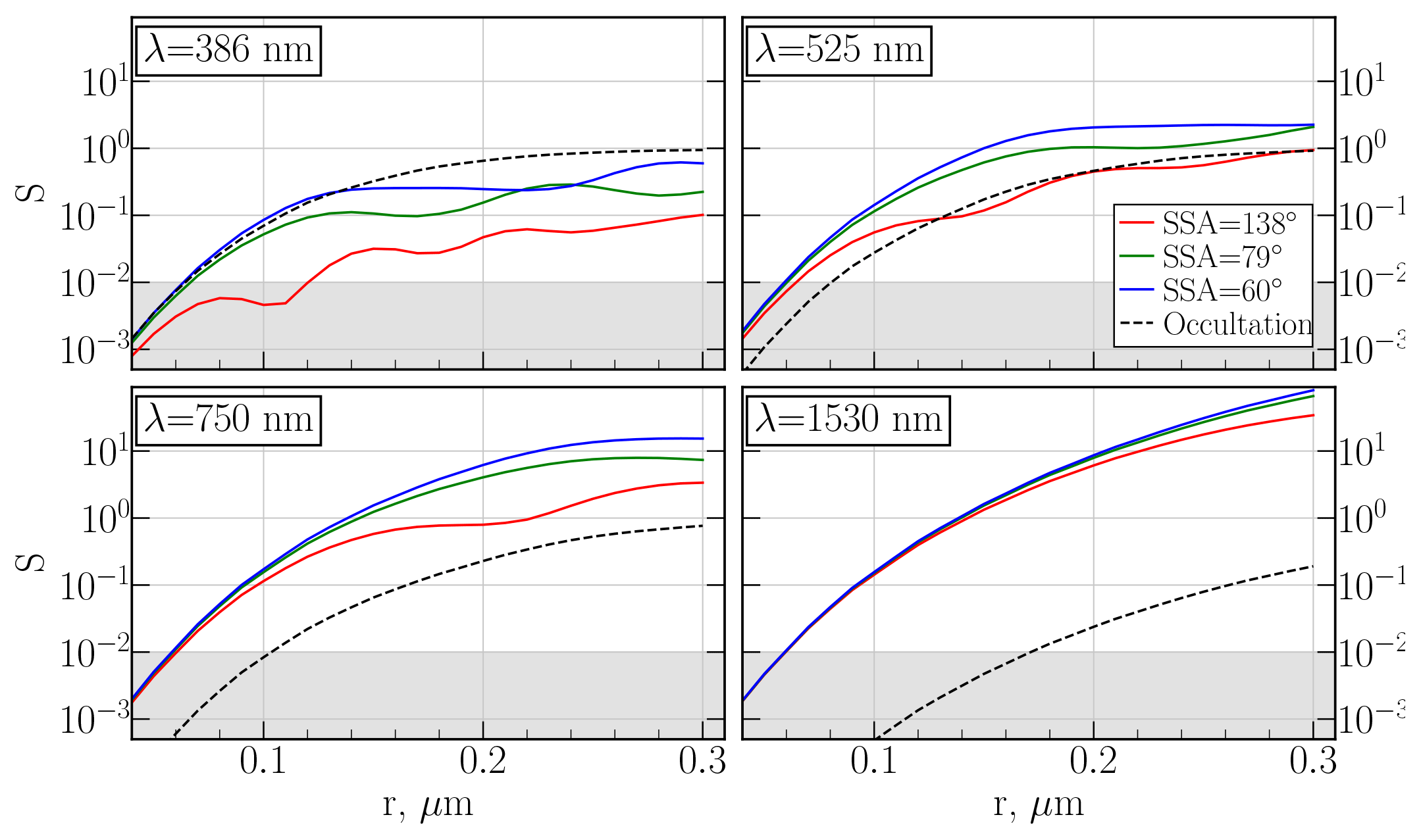
Figure 1Modelled sensitivity, S, at 21.7 km for the range of particle radii (r). The simulations were performed for different limb geometries with different solar scattering angles, SSA, and for one occultation geometry.
To understand how the differences in the measurement techniques influence the instrument sensitivity to aerosols, extended analysis is provided below. In some previous studies (e.g Twomey, 1977; Thomason and Poole, 1993; Rieger et al., 2014) the analysis of so-called kernels was used to show the contribution of the particles of different sizes to the observed radiance. According to Twomey (1977) the measured intensity of the scattered light can be presented as
where r is the radius of the particle and Ksc is a kernel. For the measurements of the transmitted light the following equation is appropriate (Twomey, 1977):
Whereas for the measurements of scattered solar light Ksc does not have an analytic representation, for the occultation measurements kernel Kdir is given by r2Qe(r∕λ), where Qe is the Mie extinction efficiency. In addition, the right sides of Eqs. (7) and (8) have the same form, although they refer to different left sides. Indeed, for the scattered light measurements the left side is represented by I(λ), while for the transmission the left side is ln (I(λ)∕I0(λ)), which according to Eq. (5) is . Thomason and Poole (1993) derived Kdir for the extinction measurements from SAGE II. In their research Kdir had units of reciprocal metres, since they were assessing it per unit volume of air. For the limb measurements, Ksc was derived for the single-scatter radiance by Rieger et al. (2014). In their work, Rieger et al. (2014) did not use Eq. (7) directly, but assessed the kernels for the measurement vector , where Iaer and IR are aerosol and Rayleigh radiance contributions. Thus, the resulting Ksc was dimensionless. It should also be noted that for their study Rieger et al. (2014) preferred to calculate Ksc for OSIRIS numerically, stating that the derived formula contains too many approximations. Thereby, kernels can be used in the assessment of the sensitivity of the instruments employing the same measurement technique, but are not suitable for the inter-instrumental comparisons. As one objective of our study is the comparison of the sensitivities of the limb and occultation measurements to the particles of the different sizes, we will not follow the approach of Twomey (1977). Instead, we define the dimensionless measurement sensitivity, S, to the aerosol particles of a certain size as a change in the intensity of the observed radiation with respect to the aerosol-free conditions. Thus, S is defined by
where I(λ) is the radiance including both, Rayleigh and aerosol signals, and IR is the Rayleigh signal. When S=0, the radiance has no contribution from the aerosol extinction or scattering. With increasing S the aerosol contribution to the measured radiance increases. The quantitative assessment of S is made by modelling the intensities with the radiative transfer model SCIATRAN (Rozanov et al., 2014) for limb measurements (using SCIAMACHY limb geometries) and for occultation measurements. The intensities were modelled for the distributions with Rmod varying from 0.04 to 0.30 µm with the step (Δr) of 0.01 µm. In accordance with the chosen Δr, for each distribution, σ has been chosen such that w is equal to 0.01 µm (e.g., Rmod=0.10 µm, σ=1.10; Rmod=0.15 µm, σ=1.07; Rmod=0.20 µm σ=1.05). The same background N profile was used for all simulations.
For the above-described simulations S at λ=386 nm, λ=525 nm, λ=750 nm and λ=1530 nm are presented in Fig. 1 for occultation (dashed black line) and for limb measurements (coloured solid lines). As limb radiances depend on SSA, the simulations were performed for three different observational geometries: SSA (blue line), SSA (green line) and SSA (red line). The angles from 60 to 140∘ represent the SSA range for SCIAMACHY measurements in the tropical region. The calculations were carried out using an ozone climatology for the month and location of the SCIAMACHY measurements. The grey shaded area shows S<0.01. We believe that this empirical value stays the same for a typical uncertainty of the measurement-retrieval system, caused by the uncertainties in the radiative transfer modelling. A justification for this is provided further in this section.
As it is seen from Fig. 1, S for limb radiances at λ=750 nm and λ=1530 nm are obviously higher than those for the occultation measurements. For λ=525 nm, the curves representing SSA and SSA lay also above the occultation one, while the red curve (SSA ) crosses the occultation line at multiple points generally comparable by the magnitude. Moreover, for these wavelengths all the SSA limb curves enter the shaded grey area at around 0.06 µm, while the occultation curves enter this area at about 0.08 µm at λ=525 nm, 0.11 µm at λ=750 nm and 0.16 µm at λ=1530 nm. These results agree with those presented by Thomason and Poole (1993) for SAGE II measurements, and illustrate the well-known statement that the occultation measurements in visible–near-infrared spectral range are insensitive to the particles with radii smaller than 0.1 µm (see e.g., Thomason et al., 2008; Kremser et al., 2016). Considering this spectral interval, better sensitivity to the smaller particles is observed for the limb measurements, which is explained by the fact that the aerosol PSD contributes in very different ways to the observed radiances for limb and occultation measurements. While Idir depends inverse exponentially on k (or Ext), Isc is, to the first order, proportional to the product of p and η. Both, p and η, depend on the PSD parameters. As a result, in the considered spectral region, limb radiances tend to be more sensitive to aerosol particles of a smaller size, and thus provide more accurate PSD parameters during the “background” aerosol loading conditions. It should be noted that at shorter wavelengths the situation is different. Thus, for λ=386 nm presented in Fig. 1 the limb curves lay below the occultation curve for all geometries. Additionally, SSA , SSA and occultation lines cross the low-sensitivity area at around r=0.06 µm, while the red line crosses the grey area at r=0.12 µm. Such a change in the sensitivity for the short wavelengths is determined by the fact that for limb measurements the Rayleigh signal in this spectral range dominates (e.g., Bourassa et al., 2012). At the same time, for the occultation measurements, inclusion of this wavelength in the PSD retrieval might be useful for the volcanically quiescent periods.
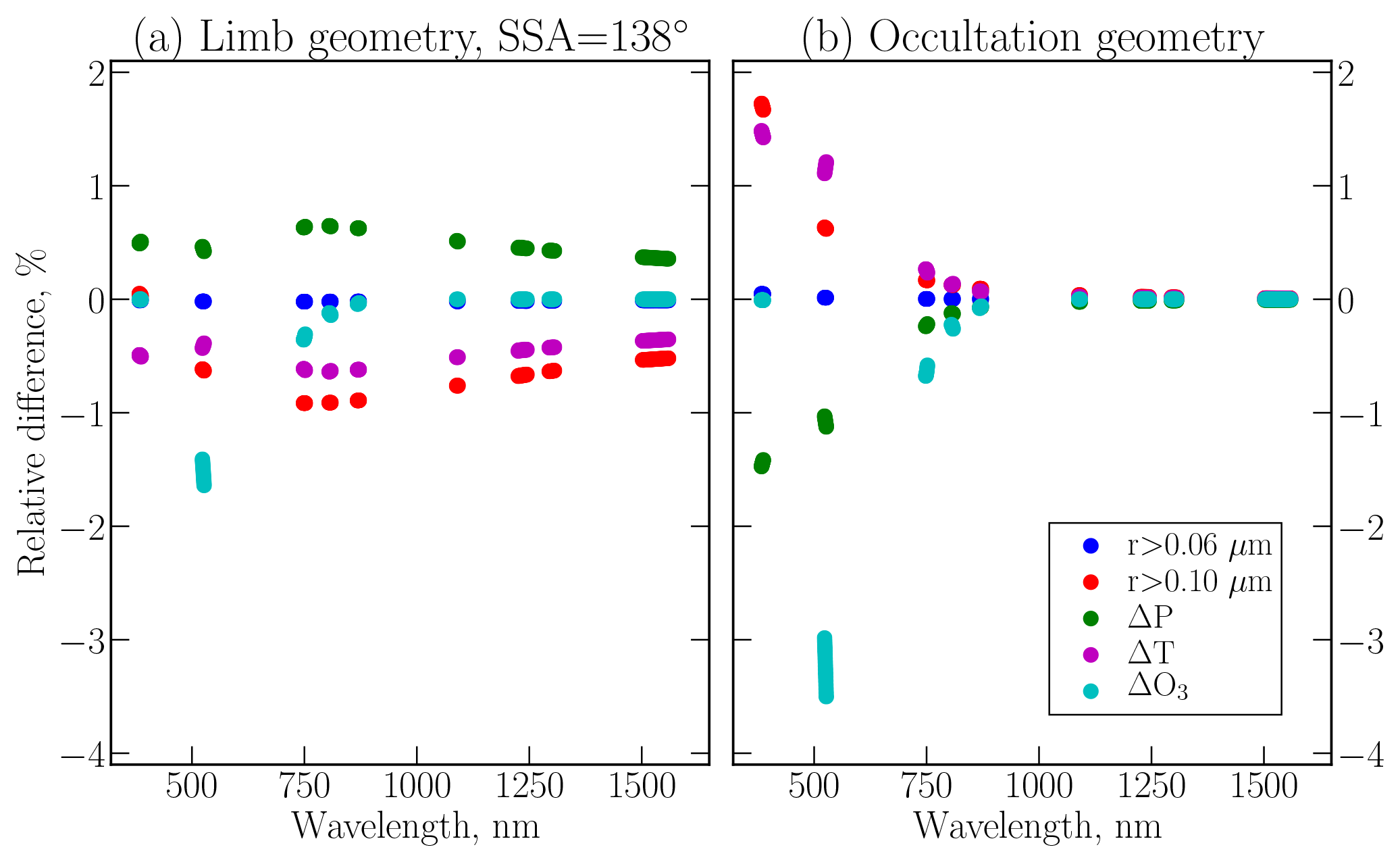
Figure 2Relative changes in the radiance at 21.7 km for limb (a) and occultation (b) geometry. The responses in radiance due to 10 % changes in temperature and atmospheric pressure and 5 % changes in ozone concentration are presented by magenta, green and cyan dots, respectively. The cutoff in PSD at 0.06 µm is depicted with blue dots, and the cutoff at 0.10 µm is presented with red dots.
To justify the choice of the sensitivity threshold, we provide an example of the relative differences in the modelled radiance due to changes in different factors for both, limb (SSA ) and occultation, geometries assuming randomly picked PSD with Rmod=0.08 µm and σ=1.6. These relative differences at 21.7 km for different wavelengths are presented in Fig. 2, with the results for limb geometry depicted in panel (a) and for occultation geometry in panel (b). For the simulations the whole profile of either temperature (magenta dots) or atmospheric pressure (green dots) was increased by 10 %. This perturbation is related to the estimated uncertainties of these parameters in the stratosphere. In the additional simulation, ozone concentration (cyan dots) was enhanced by 5 %. Changes in ozone concentration by 5 % are reasonable as they reflect the remaining uncertainties in the ozone profiles retrieved from the space-borne measurements across the relevant altitude range (Tegtmeier et al., 2013). For simplicity reasons, we perturb the whole profile, rather than values at the particular altitudes. Additionally, we depicted with the blue dots the changes in the radiances by assuming the concentration of the aerosol particles with µm equal to zero (cut off at 0.06 µm) and with the red dots assuming the cut off at 0.10 µm (particles with µm were not considered). Figure 2 shows that for the limb geometry the relative changes in the radiance due to changes in temperature, pressure or ozone concentration are within 0.8 % for most wavelengths. The exception is the 525 nm wavelength, where changes in the ozone concentrations are about 1.5 %. For the PSD cutoff at 0.06 µm the changes are about 0.03 %; however, for the cutoff at 0.10 µm the changes are about 1 % between 700 and 1000 nm, and decreasing to 0.6 % at the longer and shorter wavelengths. For the occultation geometry the changes are somewhat different. Namely, the changes in pressure or temperature are comparable with the changes in the PSD cutoff for all wavelengths, but the changes in ozone concentration contribute up to 3.5 % in the radiance at 525 nm and 1.4 % at 750 nm. Such behaviour of relative changes in the intensities shows that in the considered wavelength interval 1 % provides a realistic estimation of the uncertainties from the radiative transfer modelling for both geometries, even though this uncertainty is caused by different factors. Summarizing Sect. 3.2, it can be concluded that due to differences in the underlying radiative transfer processes, limb and occultation instruments have intrinsically different sensitivity to stratospheric aerosol parameters. Limb radiances are more sensitive to the smaller aerosol particles when measurements in the visible and near-infrared wavelength intervals are used. This is expected to result in a more accurate PSD parameter retrieval if this spectral range is used. This is particularly the case during the background aerosol loading periods when smaller particles prevail. Ext retrieval from limb instruments suffers from uncertainties due to assumed PSD and SSA dependency. Conversely, the retrieval of Ext from the occultation radiances is more straightforward, but the threshold of the sensitivity of the occultation measurements to the aerosol particle sizes is somewhat lower in comparison to the limb instruments. More information on the smaller particles from the occultation measurements can be obtained if the ultraviolet part of the spectrum is considered.
4.1 Extinction coefficient errors
As discussed above, aerosol extinction coefficient databases are widely used in stratospheric aerosol research. In order to make the SCIAMACHY aerosol PSD product comparable with the products from other satellite instruments, Ext values at four wavelengths were calculated and then used to derive the Ångström exponents at two wavelength pairs.
As was mentioned in Sect. 2.1, the SCIAMACHY PSD product provides Rmod and σ. These parameters were retrieved assuming a fixed N profile. Thus, during the volcanically active periods, an inadequate assumption of N results in errors in the retrieved Rmod and σ. To assess how this assumption affects resulting Ext and Ångström exponent, synthetic retrievals were performed. The limb radiances were simulated with the known “true” parameter settings and then used in the retrieval instead of the measurement spectra. Applying this approach, Malinina et al. (2018) showed that Rmod was retrieved with an accuracy of about 20 % even if the true value of N was a factor of 2 higher than the value assumed in the retrieval. For scenarios with the perturbed N profile, σ is retrieved with about 10 % accuracy, while an accuracy of about 5 % is reached for the profiles with unperturbed N.
To extend the error assessment of the SCIAMACHY PSD product, we use the same scenarios and the same modelled radiances as Malinina et al. (2018) to evaluate noise and parameter errors in Ext resulting from the errors in the retrieved Rmod and σ. For this study Ext was calculated employing Mie theory and Eq. (3) at 525, 750, 1020 and 1530 nm using the retrieved PSD information and the N profile assumed in the retrieval (exponentially decreasing from 15.2 cm−3 at 18 km to 0.5 cm−3 at 35 km). In addition, Ext750 was retrieved from the simulated radiances using an algorithm similar to SCIAMACHY v1.4 (Rieger et al., 2018), but with the normalization to the solar spectrum and using the phase function that was calculated from the retrieved Rmod and σ at each altitude. For this retrieval the albedo value was set to the value resulting from the PSD parameter retrieval. To distinguish the two approaches to calculate extinctions, we denominate Ext, obtained with Eq. (3) as “calculated”, and Ext, retrieved using the corrected PSD as “retrieved”.
Five scenarios for a typical observational geometry in the tropical region were used. Four of them, small, background, unperturbed and volcanic, were simulated with the same N profile as the one used for the retrieval and the aerosol PSD parameters listed in Table 1. For the scenario volcanic (2N) the N profile was multiplied by the factor of 2 below 23 km (as discussed in Malinina et al., 2018, this approach is considered to be realistic for the SCIAMACHY operation period). The scenarios are summarized in Table 1. For all scenarios the surface albedo was set to 0.15 at all wavelengths (perturbed by 0.35 in comparison to the first guess value 0.5). The measurement noise was simulated by adding the Gaussian noise to the simulated radiances. The signal-to-noise ratios were assessed from the SCIAMACHY measurements. The retrievals were carried out using 100 independent noise sequences to ensure reliable statistics.
Panel (a) of Fig. 3 shows the median calculated Ext750 profiles with solid lines and median retrieved Ext750 profiles with dashed lines. The true values are shown by the dotted lines. The colours corresponding to each scenario are listed in Table 1. Panel (b) shows the median relative parameter errors for both calculated and retrieved Ext750. Solid shaded areas show ±1 standard deviation for the calculated profiles, while the striped ones denote ±1 standard deviation for the retrieved profiles. The maximum relative errors for the calculated aerosol extinction coefficients at other wavelengths are presented in Table 1. As the altitudinal behaviour of the extinction coefficients at the other wavelengths is the same as for the Ext750 profiles, we show the results only for one wavelength.
Table 1Selected scenarios and associated maximum relative parameter errors in the calculated extinction coefficients.
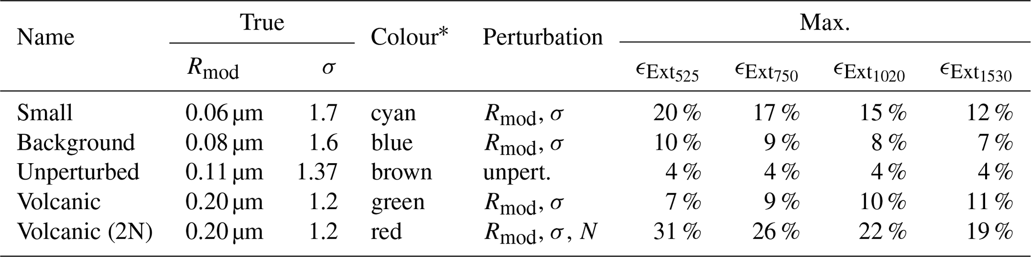
* Colour of the lines in Fig. 3.
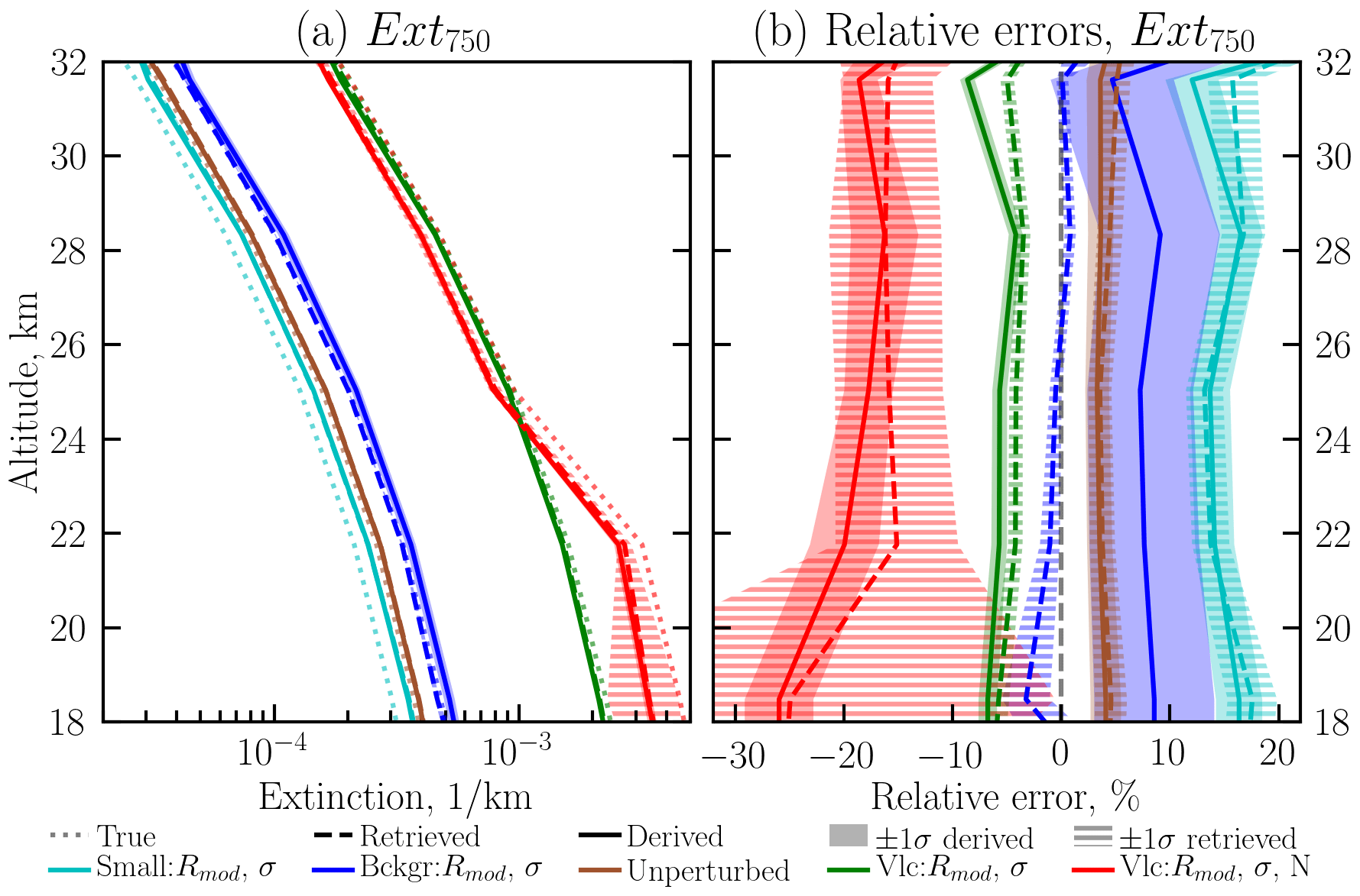
Figure 3Profiles of Ext750 (a) and their relative parameter errors (b) for a typical tropical observation geometry. The solid lines show the Ext750 profiles calculated from the PSD product. Dashed lines depict the directly retrieved profiles, while the dotted lines represent the true values. The shaded areas stand for ±1 standard deviation. The scenarios used for the simulations are listed in Table 1.
As it follows from Table 1, the relative parameter errors for the scenarios with unperturbed N do not exceed 20 %. As expected, for the volcanic (2N) scenario, the errors are slightly higher and vary depending on the wavelength from 19 % to 31 %. For all scenarios the largest parameter errors are observed for Ext525. This is most likely because for the retrieval of PSD parameters only the wavelengths longer than 750 nm were taken into consideration, while the information from the visible and UV parts of the spectrum has no contribution to the retrieval.
Analyzing Fig. 3 it is important to mention that retrieved Ext750 barely differs from that calculated. For small, unperturbed and volcanic scenarios the solid and dashed lines are very close to each other, and the median relative errors of the retrieved profiles lay mostly inside the standard deviation of calculated profiles. For the background conditions the retrieved and the calculated profiles have the same shape, but the retrieved profiles are about 8 % more accurate. As it was suggested that the difference between calculated and retrieved profiles of Ext might possibly be used to correct N for the PSD retrieval, it is most important to analyze the Ext profiles for the scenario with the perturbed N profile (volcanic (2N)). As can be seen from Fig. 3a, the retrieved Ext750 shows similar altitudinal behaviour as the calculated profile, although the retrieved profile has a larger standard deviation at the lowermost altitude. Similarly to the calculated profile, the retrieved profile is about 25 %–30 % lower than the true one. This leads to the conclusion that an additional retrieval of Ext with the corrected PSD or fixing Ext during the retrieval does not provide any additional information about the aerosol PSD, and some other independent data or constraint are needed to retrieve all three parameters. One possible way would be to combine limb and occultation measurements, using the latter to constrain N. Another possibility to constrain N would be through the use of collocated profiles of stratospheric H2SO4 concentrations. For SCIAMACHY the use of the MIPAS (Michelson Interferometer for Passive Atmospheric Sounding) H2SO4 volume mixing ratio data set (Günther et al., 2018) might be appropriate. However, synergistic use of the data from two different instruments is not straightforward, and is a subject for further studies.
4.2 Ångström exponent errors
Combining Eqs. (3) and (4), the Ångström exponent can be obtained as
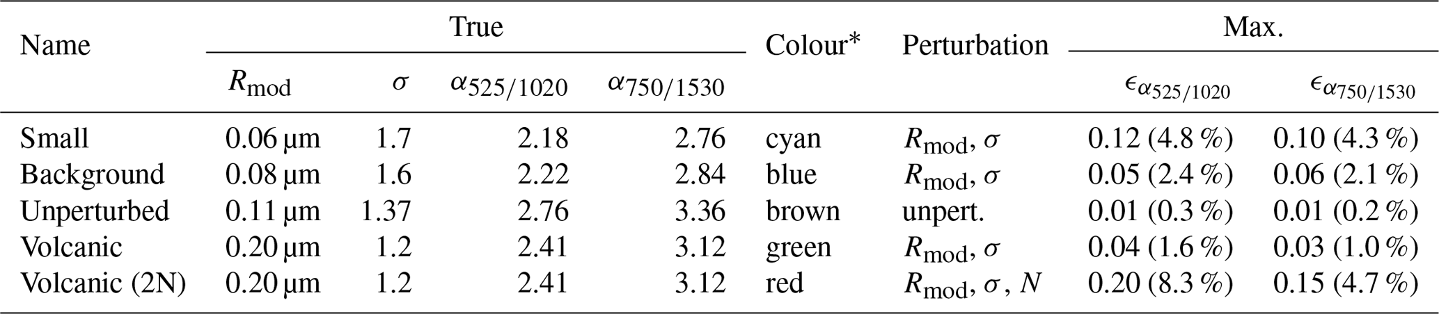
Equation (10) shows that Ångström exponent is not directly dependent on N; thus only the errors from Rmod and σ influence the derived . To assess this influence, the Ångström exponents were calculated using Eq. (10) and the calculated Ext from the synthetic retrievals discussed in Sect. 4.1. While from SCIAMACHY PSD product the Ångström exponents can be calculated at any wavelength pair, SAGE II and OSIRIS provide only α525∕1020 and α750∕1530 respectively. Thus, we limit our analysis to those values. The true Ångström exponent values, the scenario summaries (described in the previous section), and the maximum absolute and relative parameter errors for α525∕1020 and α750∕1530 are presented in Table 2. As for Ext analysis, we show the altitudinal behaviour only for one wavelength pair (α750∕1530), while the results for the other pair are very similar. In panel (a) of Fig. 4 the median derived Ångström exponents are presented with solid lines, and the true values are shown by dashed lines; in panel (b) median relative parameter errors for the chosen scenarios are depicted. For both panels shaded areas show ±1 standard deviation.
Analysis of Table 2 and Fig. 4 leads to the conclusion that the relative parameter error in the Ångström exponent for all scenarios is below 10 % for α525∕1020, and less than 5 % for α750∕1530. As expected, the largest errors are seen for the volcanic (2N) scenario, where N profile was perturbed and the parameter errors in Rmod, σ and Ext were the largest. For all scenarios the largest errors are observed at the lowermost retrieved altitude; e.g., for α750∕1530 the errors above 21.3 km do not exceed 2.5 %. The absolute error for α525∕1020 is less than 0.12 for the scenarios with unperturbed N and about 0.2 for the scenario with N perturbed by a factor of 2. For α750∕1530 the absolute parameter errors are even smaller; in particular, for the scenarios with the same N as used for the retrieval, the errors are smaller than 0.1, and for the volcanic (2N) scenario the difference between the true and derived Ångström exponents is 0.15.
Table 2Selected scenarios and associated maximum absolute (relative) parameter errors in Ångström exponents.
* Colour of the lines in Fig. 4. In the last two columns maximum absolute error for the profile is given by the number without brackets, while the maximum relative error is presented in brackets.
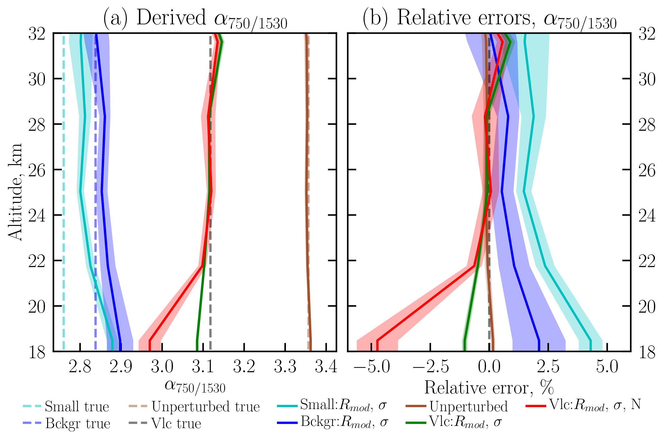
Figure 4Ångström exponent profiles (α750∕1530) (a) and their relative parameter errors (b) for a typical tropical observation geometry. The solid lines show the profiles derived from the PSD product, while the dashed lines represent the true values. The shaded areas stand for ±1 standard deviation. The scenarios used for the simulations are listed in Table 2.
Summarizing Sect. 4, it can be concluded that parameter errors in the calculated Ext for the background scenarios do not exceed 20 %, and are about 20 %–25 % for the cases with the perturbed N. The largest errors are observed for the aerosol extinction coefficient at 525 nm, most likely due to the missing information from the visible spectral range in the PSD retrieval. The retrieval results for Ext with the retrieved PSD parameters barely differ from the aerosol extinction coefficients calculated from the PSD product, and thus cannot be used to improve the knowledge of N. For the Ångström exponent the parameter errors are much smaller, as they cancel out in the ratio of the aerosol extinction coefficients and depend only on the aerosol PSD. For α525∕1020 the relative parameter error does not exceed 10 %, and for α750∕1530 the relative error is below 5 %. For both Ångström exponents the absolute parameter errors are less than 0.2 for the cases with the perturbed N profile and are even less than 0.1 for unperturbed N.
5.1 Extinction coefficient comparison with SAGE II
As discussed in the previous sections, SAGE II was an outstanding instrument, providing aerosol extinction coefficients, and there have been several comparisons performed using its data. For the SCIAMACHY PSD product the comparisons with SAGE II are associated with some challenges. First, SCIAMACHY and SAGE II have only a 3-year period of overlap. Second, SAGE II was an occultation instrument, providing about 30 vertical profiles per day, which resulted in 57 collocated profiles with SCIAMACHY (collocation criteria are latitude, longitude and ±24 h) for the entire overlap period because the SCIAMACHY PSD retrieval is currently limited to completely cloud-free profiles in the tropical zone (20∘ S–20∘ N). This number of collocated profiles is not enough for an in-depth investigation; however a rough assessment of the consistency of the data from both instruments can be provided. Another issue related to the SCIAMACHY and SAGE II comparison is the difference in the measurement techniques and thus a different sensitivity to aerosol properties. As was discussed in Sect. 3.2, SAGE II as an occultation instrument using visible–near-infrared spectral information for the PSD assessment is less sensitive to the smaller particles. At the same time, Ext retrieval from SAGE II is associated with smaller uncertainties. The limb measurements from SCIAMACHY, in turn, are more sensitive to the particles with r<0.10 µm, although the direct retrieval of Ext is associated with some issues (see Sect. 3.2). The comparison of the reff from SAGE II and SCIAMACHY, presented in Malinina et al. (2018) is expected to be influenced by these differences because the instruments' overlap period is considered to be volcanically quiescent with a prevailing number of smaller particles. Here, we present the comparison of Ext retrieved from SAGE II and that calculated from the SCIAMACHY PSD product, which is expected to be more reliable than a direct comparison of reff.
To perform the comparison, SCIAMACHY aerosol extinction coefficients at 525, 750 and 1020 nm were calculated with Eq. (3), considering the same N profile as used in the PSD retrieval. As SAGE II did not have a 750 nm channel, Ext750 for this instrument was calculated with Eq. (4) from Ext525 and Ext1020 using α525∕1020. To assess a possible uncertainty associated with the usage of the Ångström exponent when calculating Ext750 from SAGE II data, SCIAMACHY Ext750 was additionally calculated using the same approach. To distinguish between two different methods of Ext750 calculation, we use Ext750(PSD) for the one derived from the PSD product with Eq. (3) and Ext750(α525∕1020) for that calculated using the Ångström exponent. As SCIAMACHY and SAGE II have different vertical resolutions, SAGE II data were smoothed to the coarser SCIAMACHY vertical resolution and then interpolated onto the SCIAMACHY vertical grid. The mean relative differences between SCIAMACHY and SAGE II for Ext525 (blue line), Ext1020 (green line), Ext750(PSD) (red line) and Ext750(α525∕1020) (magenta line) are presented in Fig. 5. The shaded areas show the standard error of the mean. We prefer to depict the standard error of the mean instead of the standard deviation to make the figures less busy.
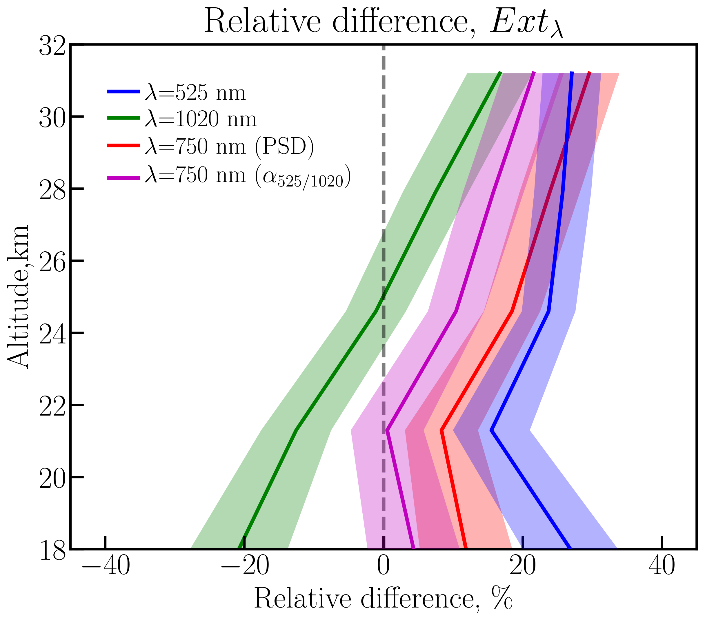
Figure 5Mean relative difference (200×(SCIAMACHY-SAGE II)/(SCIAMACHY+SAGE II)) between extinction coefficients at 525 nm (blue line), 1020 nm (green line) and 750 nm obtained directly from PSD (red line) and 750 nm converted with α525∕1020 (magenta line) from collocated SCIAMACHY and SAGE II measurements. Shaded areas show standard error of the mean.
As can be seen from Fig. 5, for all wavelengths the differences for the derived extinction coefficients are below ±25 %, which is within the reported precision of the extinction coefficients for SCIAMACHY. For Ext1020 the shape of the relative difference follows the one reported earlier in Malinina et al. (2018) for the differences between SCIAMACHY and SAGE II effective radii, but with slightly different values (−20 % to 10 % for Ext1020 versus −30 % to 0 % for reff). Such behaviour is expected because reff from SAGE II is obtained using Ext1020 and Ext525 (see Sect. 2.3). The differences in Ext525, Ext750(PSD) and Ext750(α525∕1020) are fairly constant with height and vary from 15 to 25 % for Ext525, from 10 % to 25 % for Ext750(PSD) and from 0 to 15 % for Ext750(α525∕1020). The discrepancy between two different ways of computing Ext750 is quite remarkable, as with the consistent methods a better agreement is obtained. Though it should be highlighted once again that for SAGE II 750 nm is not a measurement wavelength, and 525 nm is not considered in the SCIAMACHY retrieval. To highlight the uncertainties coming from the different approaches to derive Ext750, we depict in Fig. 6 the mean relative differences between Ext750(α525∕1020) and Ext750(PSD) for the whole SCIAMACHY data set with a solid line, and ±1 the standard deviation is shown as the shaded area. From Fig. 6 it is clear that the calculation of the extinction coefficient with Ångström exponent results in about 8 % negative bias. This result is consistent with the result presented in the supplements to Rieger et al. (2015). Thus, it is important to consider this uncertainty when comparing the aerosol extinction coefficients from different instruments measuring at different wavelengths.
Figure 6Mean relative difference between Ext750(PSD) obtained from the PSD product with Eq. (3) and Ext750(α525∕1020) calculated using the Ångström exponent (100× (Ext750(α525∕1020)-Ext750(PSD))/Ext750(PSD)) from all available SCIAMACHY measurements. The shaded area shows the ±1 standard deviation.
5.2 Ångström exponent comparison with SAGE II
To extend the comparison to the data from SAGE II, α525∕1020 was calculated from its aerosol extinctions and compared to the ones derived from the SCIAMACHY PSD product. The mean differences between SCIAMACHY and SAGE II Ångström exponents are presented in Fig. 7 with the solid blue line, with relative differences in panel (a) and absolute differences in panel (b). Following the previous comparison, the standard error of the mean is shown with the shaded area.
The relative difference between the instruments is altitude dependent, showing a different shape than Ext1020. SCIAMACHY α525∕1020 is about 40 % higher than that from SAGE II at 18 km, about 20 % higher between 21 and 28 km, and the difference at 31 km is around 10 %. In the absolute values the difference varies from 0.8 at the lowermost altitude to 0.2 at the uppermost one. The observed differences in this comparison are expected. As was discussed in the previous section, the differences between SCIAMACHY and SAGE II for Ext1020 and Ext525 are both about 20 %, but have the opposite sign, which results in the amplification of the error when calculating α525∕1020. As for reff and Ext1020, the reason why the difference between SCIAMACHY and SAGE II is altitude dependent is still under investigation. To address this question the number of collocations needs to be significantly increased to provide better sampling. This can be done by extending the SCIAMACHY PSD retrieval algorithm to other latitude bands and applying it to the profiles with cloud contamination.
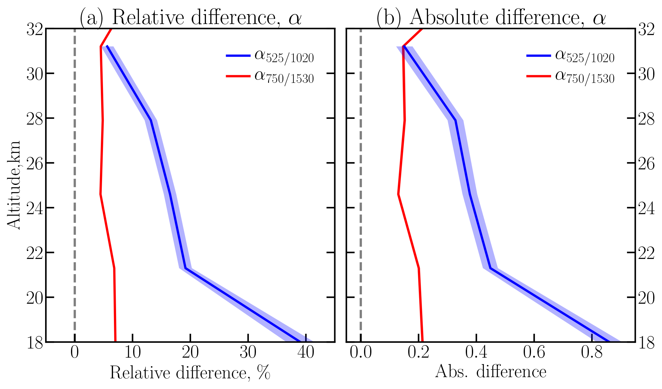
Figure 7Mean relative (a) and absolute (b) differences (200× (SCIAMACHY-instrument)/(SCIAMACHY+instrument)) between Ångström exponents from collocated SCIAMACHY and SAGE II (α525∕1020: blue lines) and SCIAMACHY and OSIRIS (α750∕1530: red lines) measurements. Shaded areas show standard error of the mean.
5.3 Ångström exponent comparison with OSIRIS
Although comparison of SCIAMACHY with SAGE II provides some information on the agreement of the products, this comparison is not sufficient to draw any robust conclusions. Additional information can be gained from the comparison with OSIRIS, which was operating at the same time as SCIAMACHY and also provided particle size information. Generally, comparison between SCIAMACHY and OSIRIS is more robust than with SAGE II, as both instruments employ the same measurement technique, use information at the same wavelengths (750 and 1530 nm) and provide a similar number of measurements per orbit. Applying the same collocation criteria as for SAGE II, 4603 coincident profiles were found, which is about half of the available SCIAMACHY profiles. The obtained number of collocations is sufficient to ensure a reliable comparison. It is important to highlight once again that all the comparisons were performed for the tropical region (20∘ N–20∘ S).
Differences between SCIAMACHY and OSIRIS α750∕1530 are presented in Fig. 7 by the red line. OSIRIS α750∕1530 was interpolated onto the SCIAMACHY measurement grid. The difference in vertical resolution was not accounted for as SCIAMACHY and OSIRIS have similar specifications. As for SAGE II, in panel (a) of Fig. 7 the mean relative differences are plotted with a solid line, while in panel (b) the mean absolute differences are depicted. The standard error of the mean is shown by the shaded area; it is, however, within the thickness of the solid line. As follows from Fig. 7, the relative difference between SCIAMACHY and OSIRIS is about 7 % for the lower altitudes and about 4 % for the altitudes above 25 km. In absolute values the difference is about 0.2 below 25 km, and less than 0.15 at the higher altitudes. Taking into consideration the α750∕1530 errors from SCIAMACHY (5 %), estimated in Sect. 4.2, and the errors reported by Rieger et al. (2014) for OSIRIS Ångström exponents (10 %), it can be concluded that the Ångström exponents obtained from both instruments agree well, with the difference being smaller than the reported errors.
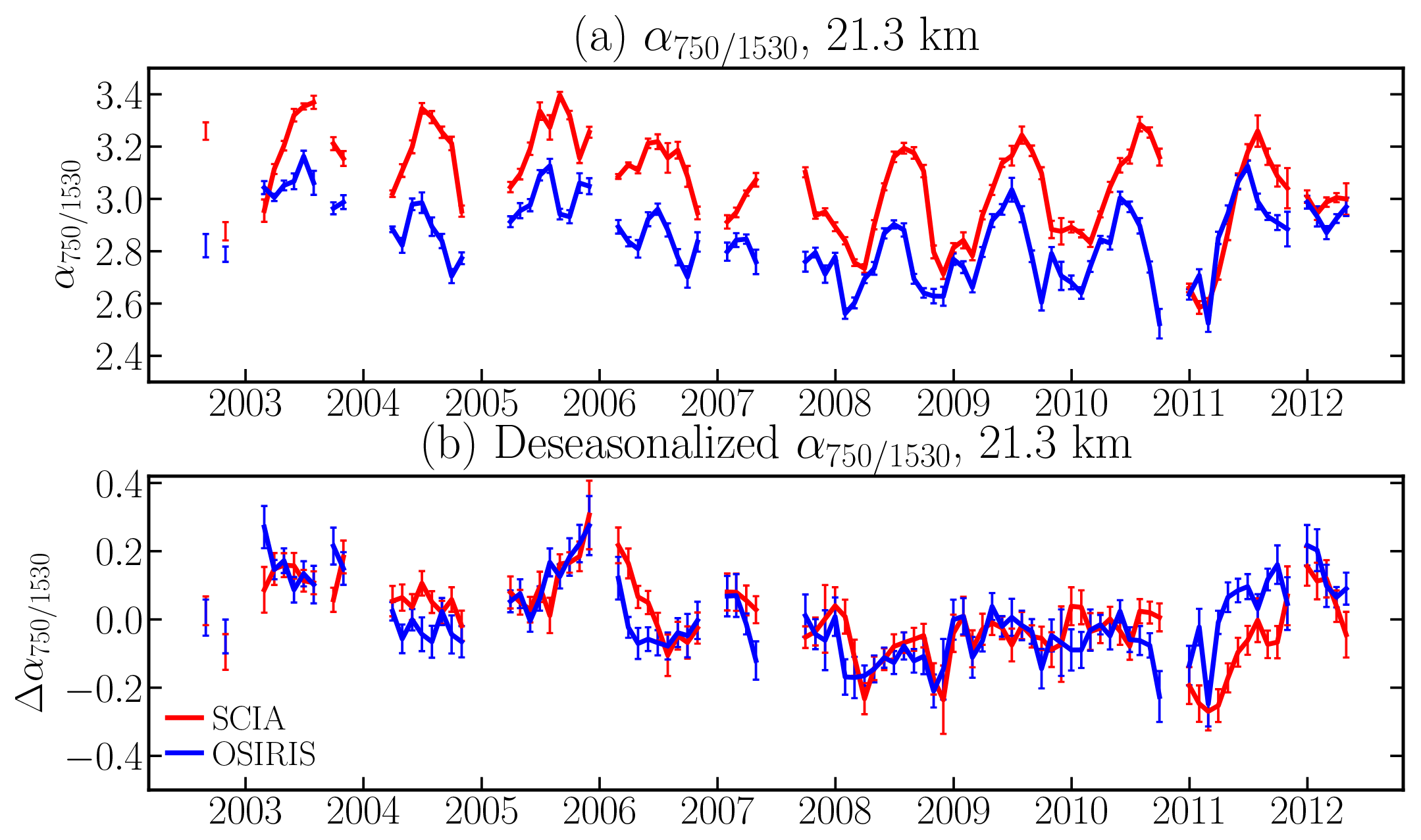
Figure 8Zonal monthly mean (a) and deseasonalized (b) Ångström exponents (α750∕1530) from collocated SCIAMACHY and OSIRIS measurements. Vertical bars show standard error of the mean.
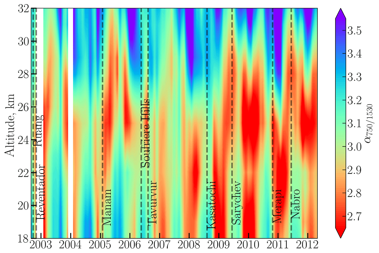
Figure 9Monthly zonal mean values of the Ångström exponents (α750∕1530) derived from SCIAMACHY limb data in the tropics (20∘ N–20∘ S).
To evaluate the temporal behaviour of the differences between SCIAMACHY and OSIRIS results, the monthly zonal means of α750∕1530 and its deseasonalized values (anomalies) at 21.3 km are plotted respectively in panels (a) and (b) of Fig. 8. The deseasonalization of α750∕1530 for the both instruments is justified, firstly, by the seasonality of stratospheric aerosols, which was reported in multiple studies including Hitchman et al. (1994) and Bingen et al. (2004), and secondly by the dependency of the limb radiances on the seasonal changes in SSA. The deseasonalized values for each instrument were calculated individually by subtracting an averaged α750∕1530 over all corresponding months in the whole observation period from each monthly mean value (e.g., the averaged α750∕1530 for July every year from 2002 until 2012 was subtracted from the monthly mean value of each July in 2002–2012). Months with fewer than 10 collocations were excluded from the comparison. SCIAMACHY data are presented in red and OSIRIS in blue; the vertical bars show the standard error of the monthly mean value.
As seen in panel (a) of Fig. 8, the Ångström exponents retrieved from both instruments show very similar behaviour, although the absolute values of α750∕1530 from SCIAMACHY are systematically higher than those from OSIRIS. A high degree of consistency is found between the results from both instruments in the comparison of the deseasonalized time series (see panel b of Fig. 8). Generally, the blue and red lines overlap or lay within the error bars and follow the same pattern, except at the beginning of 2006, when SCIAMACHY values are slightly higher, and 2011, when OSIRIS is slightly higher. However, even in those periods the differences are rather small (about 0.05–0.08). As the differences between Ångström exponents from both instruments are fairly constant with time, and do not show signatures of any remarkable events (e.g., volcanic eruptions), it can be concluded that they originate most probably from the technical specifications of the instruments and differences in the retrieval algorithms.
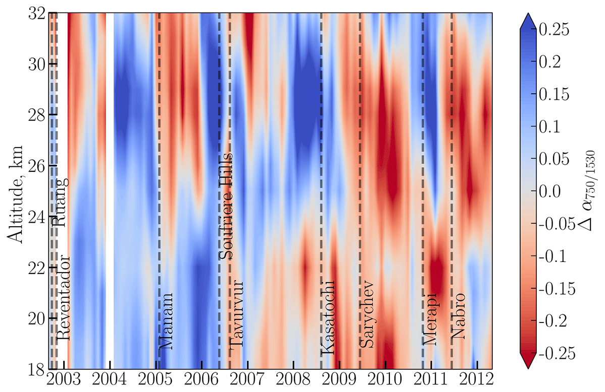
Figure 10Deseasonalized time series (anomalies) of the Ångström exponents (α750∕1530) derived from SCIAMACHY limb data in the tropics (20∘ N–20∘ S).
Summarizing Sect. 5, the following conclusions are made: aerosol extinction coefficients obtained from the SCIAMACHY PSD product agree with SAGE II within ±25 %, i.e., within the reported accuracy of the obtained Ext from SCIAMACHY. The best agreement was acquired for Ext750, calculated for both instruments from Ext525 and Ext1020 with α525∕1020. Additionally, it was shown that the recalculation of Ext using the Ångström exponent can result in about 8 % bias. Ångström exponents from SCIAMACHY were compared to the ones from SAGE II and OSIRIS. The differences with respect to SAGE II results are about 40 % at 18 km, decreasing to 20 % at 21 km and to 10 % at 30 km. With respect to OSIRIS, the agreement is much closer, with relative differences between 4 % and 7 %. The differences between the instruments are smaller than the expected uncertainties, showing remarkable agreement between the instruments. The temporal behaviour of α750∕1530 anomalies is independent of any remarkable events, with minor differences coming from the small technical differences of the instruments and retrievals. The much better agreement of SCIAMACHY aerosol values with OSIRIS than with SAGE II is explained by a better consistency of the data sets: the same measurement technique and the same spectral information were used to retrieve the parameters.
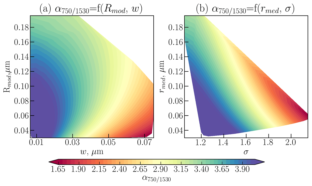
Figure 11Dependence of the Ångström exponent (α750∕1530) on mode radius, Rmod, and absolute distribution width, w (a). In panel (b) α750∕1530 as a function of median radius, rmed, and σ is presented. Plot is based on the SCIAMACHY limb data in the tropics (20∘ N–20∘ S).
In order to investigate the temporal behaviour of the Ångström exponent and to understand its dependency on the PSD parameters, the SCIAMACHY data set recalculated from the PSD product was analyzed. Unfortunately, due to rejection of cloud-contaminated profiles temporal sampling of the obtained product is too sparse to analyze volcanic plumes. For this reason the monthly zonal mean (20∘ S–20∘ N) α750∕1530 values as shown in Fig. 9 were considered. With exception of the upper altitudes (26–32 km), where the quasi-biannual oscillation (QBO) pattern is obvious, the seasonal variation in α750∕1530 represents the dominating pattern seen in Fig. 9. As was mentioned in Sect. 5.3, the seasonality of stratospheric aerosols was discussed in several previous studies. To make the analysis of the Ångström exponent behaviour after the volcanic eruptions more clear, α750∕1530 was deseasonalized using the same approach as discussed in Sect. 5.3. The deseasonalized α750∕1530 time series are presented in Fig. 10. It should be noted that in Fig. 10 the increased Ångström exponent values are shown in blue, and the decreased values in red, as the increased α750∕1530 is often interpreted as a decrease in the aerosol particle size, and vice versa.
Looking at Fig. 10, it becomes even more evident that the QBO pattern is well pronounced at altitudes above 26 km. This agrees with results reported earlier for SCIAMACHY aerosol products; e.g., Brinkhoff et al. (2015) showed similar patterns at around 30 km altitude for Ext750. Later, the QBO signatures in Rmod and w were revealed by Malinina et al. (2018). The deseasonalized α750∕1530 time series also demonstrate the influence of multiple volcanic eruptions. The slight decrease in α750∕1530 was noticed after the Tavurvur eruption, and more significant after the extratropical Kasatochi and Sarychev eruptions. Almost no change in α750∕1530 was observed after the Ruang, Reventador and Manam eruptions. After the Nabro eruption α750∕1530 increased at the 18–23 km altitude. As for Rmod and w from the same data set (Malinina et al., 2018), the changes in α750∕1530 reach higher altitudes with a certain time lag (tape-recorder effect). Interestingly, the general behaviour of α750∕1530 looks very similar to that of w (Malinina et al., 2018, Fig. 12). To evaluate it in more detail, the dependency of α750∕1530 on Rmod and w was analyzed.
It is well known that α750∕1530 is dependent on both rmed and σ but as Rmod and w are derived from these parameters, their impact on α750∕1530 is not obvious. To investigate these relationships, the results from individual measurements in the tropical region over the whole observation period of SCIAMACHY are presented in Fig. 11. In panel (a), α750∕1530 at all altitudes is presented as a function of Rmod and w, while in panel (b) the dependency of α750∕1530 on rmed and σ is shown. The colours in Fig. 11 depict the magnitude of α750∕1530. From Fig. 11, it is clear that any particular value of α750∕1530 can result from an infinite number of combinations of Rmod and w (or rmed and σ). However we note that retrieving a pair of Rmod∕rmed and w∕σ is not the only way to obtain the Ångström exponent. As was discussed in Malinina et al., 2018, in the spectral interval from 750 to 1530 nm the radiance can be fitted by two out of three PSD parameters, for SCIAMACHY the pair Rmod and σ was chosen as the limb radiances' sensitivity to these parameters is higher than to N. However, it is possible to obtain a correct Ångström exponent also by retrieving, rmed and N (Rieger et al., 2014), although the accuracy of the PSD parameters may not be as high as for Rmod and σ.
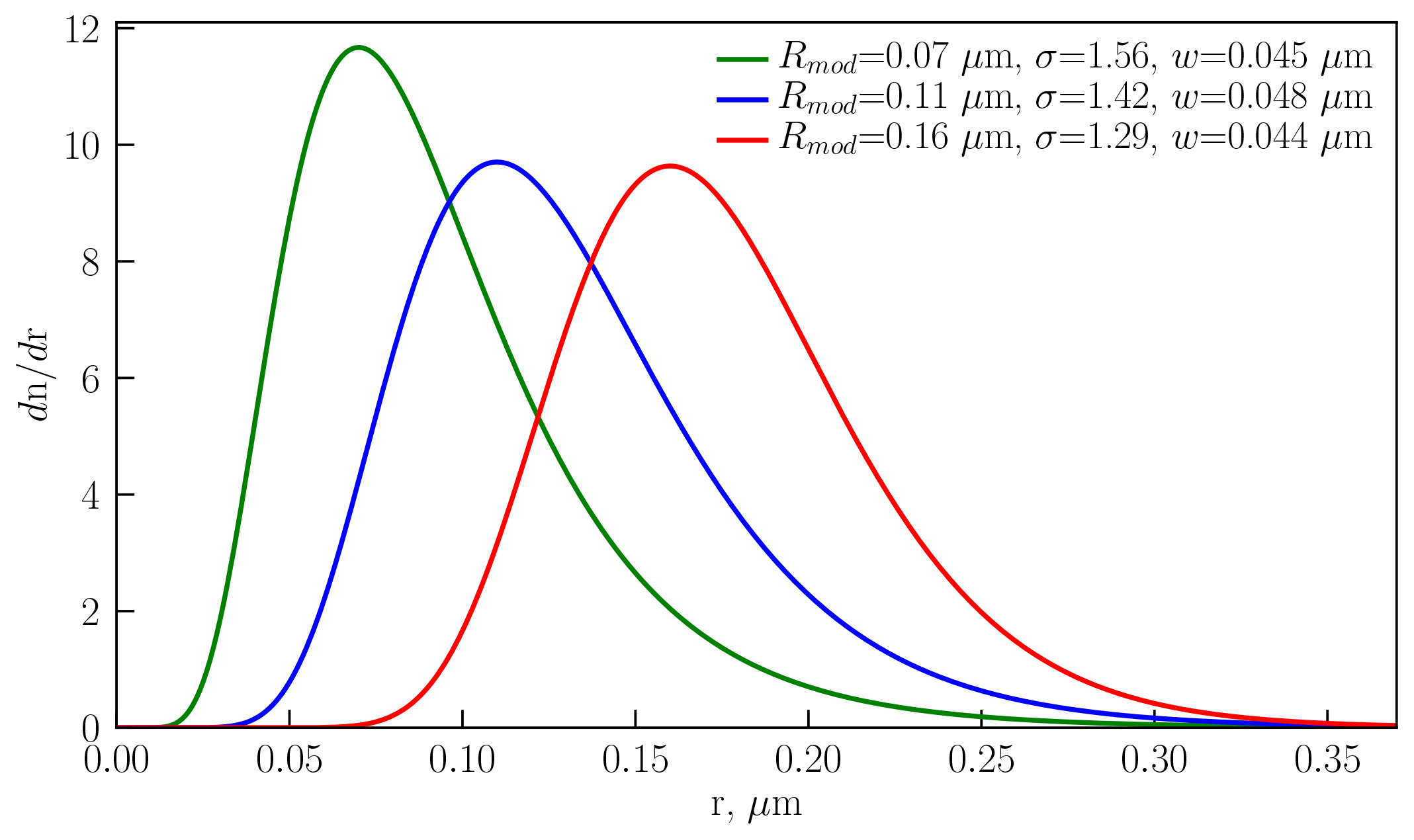
Comparing panels (a) and (b) it can be seen that is a non-monotonic function; i.e., up to a turn-around point the same value of α750∕1530 is obtained by increasing both Rmod and w, and then the same α750∕1530 is a result of increasing Rmod and decreasing w. The function is monotonic with respect to both rmed and σ, and there is the general rule: the larger rmed or σ is, the smaller α750∕1530 is. The same value of α750∕1530 can be reached by increasing rmed and decreasing σ or vice versa. It is important to highlight that completely different distributions might result in the same value of α750∕1530. To illustrate this fact, we chose three pairs of PSD parameters with , and plotted the distributions dn∕dr in Fig. 12. The values of Rmod, σ and w used for the figure are listed in the legend. This figure disproves a widely spread belief often held in scientific discussions that a smaller value of an Ångström exponent is associated with the prevalence of larger particles and vice versa. As can be seen, distributions with Rmod=0.07 µm and w=0.045 µm (green line) and Rmod=0.16 µm and w=0.044 µm (red line) have completely different numbers of large particles, but result in the same Ångström exponent. As was already noted by Ångström (1929), α has only an “approximate coincidence with the average diameter directly measured”. Thus, it can be concluded that, firstly, there is no possibility to obtain a unique pair of PSD parameters from the known single value of α750∕1530, and secondly, to provide relevant information on the change in the particle size, α750∕1530 should be accompanied by one of the PSD parameters. Here, we note that our conclusions are valid for the Ångström exponent at one wavelength pair. If several Ångström exponents for different independent wavelength pairs are provided, more information on PSD can be derived. However, any conclusions about particle size based on the Ångström exponent at one wavelength pair without any additional PSD information are meaningless. Currently, for all known space-borne instruments providing aerosol information in the stratosphere, only one value of Ångström exponent is reported in peer-reviewed publications, which makes our conclusions applicable to all of them. This statement is clearly not applicable to the data sets directly providing PSD information.
Summarizing Sect. 6, it can be concluded that based on the available climatology α750∕1530 can increase, decrease or remain unchanged after the volcanic eruptions. As for Rmod and w from the same data set, the tape-recorder effect after the volcanic eruptions as well as QBO signatures at upper altitudes (26–32 km) are observed. The pattern of α750∕1530 changes is similar to that of the changes in w, although changes in both Rmod and w contribute to the changes in α750∕1530. It was also shown, in the examples of the single measurements, that an infinite number of Rmod and w (or rmed and σ) pairs result in the same α750∕1530, and the statement that the large (small) Ångström exponent means the prevalence of small (large) particles is strictly valid only for increasing (decreasing) rmed with σ remaining unchanged.
In this study, the stratospheric aerosol extinction coefficient and Ångström exponent have been discussed. From the investigation of the sensitivity of space-borne measurements in the visible–near-infrared spectral range to the aerosol particles of different size, it was shown that limb scatter instruments are sensitive to the aerosol particles of smaller size, and thus provide more accurate PSD information than solar occultation instruments, in particular during periods with low aerosol loading. However, the sensitivity threshold of the occultation instruments can be improved, in case the UV part of the spectrum is considered. In contrast, occultation instruments provide aerosol extinction coefficients which are associated with smaller uncertainties than the ones from the limb instruments.
Here, we focus on the aerosol PSD product, which provides Rmod and σ (and recalculated w), obtained from SCIAMACHY limb measurements. In order to compare it with other space-borne instruments, aerosol extinction coefficients and Ångström exponents were recalculated using the PSD parameters. Error estimation based on the synthetic retrieval approach showed that the aerosol extinction coefficients are obtained with about 25 % accuracy for the scenarios with high aerosol loading and with less than 20 % uncertainty for the background period. It was also shown that by using the retrieved Rmod and σ from the same data set it is impossible to estimate N, or put another constraint on the parameters by implementing a coupled or consequent Ext retrieval. Ångström exponents calculated from the PSD parameters show less than 10 % error for α525∕1020 and less than 5 % error for α750∕1530. In the absolute values these errors are less than 0.2 and 0.15 respectively.
The recalculated aerosol extinction coefficients from the SCIAMACHY observations were compared to those from SAGE II. This comparison showed that differences are within ±25 %, which is within theoretically determined errors for SCIAMACHY. Ångström exponent (α525∕1020) differences vary from 40 % at 10 km to 10 % at 30 km, with SAGE II values being systematically smaller. Furthermore, SCIAMACHY Ångström exponents (α750∕1530) were compared to those from OSIRIS (another limb scatter instrument). The relative difference between the instruments is decreasing from 7 % at the lowermost altitudes to 4 % at the uppermost altitudes. The absolute values of α750∕1530 differ by less than 0.2, and both relative and absolute differences are within the theoretically determined errors of α750∕1530 for those instruments. The time series analysis of the collocated data sets showed that the differences do not change significantly with time and are not correlated with any remarkable events, such as volcanic eruptions. The Ångström exponent in the tropics was analyzed using the values recalculated from the SCIAMACHY PSD data set. It was shown that the monthly α750∕1530 anomalies show distinct QBO signatures in the upper stratosphere, and the Ångström exponent can increase, decrease or remain unchanged after a volcanic eruption. The analysis showed that changes in α750∕1530 are driven by changes in both Rmod and w (or rmed and σ), and an infinite number of pairs of these parameters provides the same value of α750∕1530. It was concluded that it is impossible to derive any reliable information on the changes in the aerosol size based solely on the Ångström exponent for one wavelength pair. This can only be done if at least one of the PSD parameters is provided in addition.
SCIAMACHY aerosol particle size distribution data are available after registration at http://www.iup.uni-bremen.de/DataRequest/ (Rozanov, 2019) The OSIRIS data set can be downloaded at http://odin-osiris.usask.ca/?q=node/280 (Roth, 2019).
EM provided the SCIAMACHY PSD data set, calculated aerosol extinction coefficients and Ångström exponents, compared the resulting product to OSIRIS and SAGE II, and wrote the paper. AR supervised and guided the work at the University of Bremen and revised the paper. LR provided the OSIRIS v6.0 data set, contributed into the comparison studies and revised the paper. AB and DD supervised the work at the University of Saskatchewan and revised the paper. HB performed scientific assurance of SCIAMACHY data quality and revised the paper. JPB initiated and proposed the research and led the project; he contributed to the data analysis, the establishment of the scientific outcomes and the preparation of the paper.
The authors declare that they have no conflict of interest.
This work was funded in part by the German Research Foundation (DFG) through the research unit VolImpact, European Space Agency (ESA) through the SQWG and SPIN projects, German Aerospace Center (DLR) through the SADOS project, German Federal Ministry of Education and Research (BMBF) through the ROMIC-ROSA project, the Natural Sciences and Engineering Research Council (Canada), the Canadian Space Agency, and the University of Bremen and state of Bremen. The Postgraduate International Programme in Physics and Electrical Engineering (PIP) and University of Bremen provided a grant for Elizaveta Malinina to visit the University of Saskatchewan. We thank ECMWF for providing pressure and temperature information. We also thank NASA for SAGE II data, which were downloaded from the NASA Langley Research Center EOSDIS Distributed Active Archive Center.
The article processing charges for this open-access publication were covered by the University of Bremen.
This paper was edited by Alexander Kokhanovsky and reviewed by two anonymous referees.
Ångström, A.: On the atmospheric transmission of sun radiation and on dust in the air, Geograf. Ann., 11, 156–166, 1929. a, b, c, d
Arosio, C., Rozanov, A., Malinina, E., Eichmann, K.-U., von Clarmann, T., and Burrows, J. P.: Retrieval of ozone profiles from OMPS limb scattering observations, Atmos. Meas. Tech., 11, 2135–2149, https://doi.org/10.5194/amt-11-2135-2018, 2018. a
Barkstrom, B. R. and Smith, G. L.: The earth radiation budget experiment: Science and implementation, Rev. Geophys., 24, 379–390, 1986. a
Bingen, C., Fussen, D., and Vanhellemont, F.: A global climatology of stratospheric aerosol size distribution parameters derived from SAGE II data over the period 1984–2000: 1. Methodology and climatological observations, J. Geophys. Res.-Atmos., 109, D06201, https://doi.org/10.1029/2003JD003518, 2004. a, b
Bingen, C., Robert, C. E., Stebel, K., Brühl, C., Schallock, J., Vanhellemont, F., Mateshvili, N., Höpfner, M., Trickl, T., Barnes, J. E., Jumelet, J., Vernier, J.-P., Popp, T., de Leeuw, G., and Pinnock, S.: Stratospheric aerosol data records for the climate change initiative: Development, validation and application to chemistry-climate modelling, Remote Sens. Environ., 203, 296–321, https://doi.org/10.1016/j.rse.2017.06.002, 2017. a
Bourassa, A. E., Rieger, L. A., Lloyd, N. D., and Degenstein, D. A.: Odin-OSIRIS stratospheric aerosol data product and SAGE III intercomparison, Atmos. Chem. Phys., 12, 605–614, https://doi.org/10.5194/acp-12-605-2012, 2012. a, b, c
Bovensmann, H., Burrows, J., Buchwitz, M., Frerick, J., Noël, S., Rozanov, V., Chance, K., and Goede, A.: SCIAMACHY: Mission objectives and measurement modes, J. Atmos. Sci., 56, 127–150, 1999. a, b
Brinkhoff, L. A., Rozanov, A., Hommel, R., von Savigny, C., Ernst, F., Bovensmann, H., and Burrows, J. P.: Ten-Year SCIAMACHY Stratospheric Aerosol Data Record: Signature of the Secondary Meridional Circulation Associated with the Quasi-Biennial Oscillation, in: Towards an Interdisciplinary Approach in Earth System Science, Springer, 49–58, 2015. a
Brühl, C., Lelieveld, J., Tost, H., Höpfner, M., and Glatthor, N.: Stratospheric sulfur and its implications for radiative forcing simulated by the chemistry climate model EMAC, J. Geophys. Res.-Atmos., 120, 2103–2118, 2015. a
Burrows, J., Hölzle, E., Goede, A., Visser, H., and Fricke, W.: SCIAMACHY-Scanning imaging absorption spectrometer for atmospheric chartography, Acta Astronaut., 35, 445–451, 1995. a, b
Chen, Z., Bhartia, P. K., Loughman, R., Colarco, P., and DeLand, M.: Improvement of stratospheric aerosol extinction retrieval from OMPS/LP using a new aerosol model, Atmos. Meas. Tech., 11, 6495–6509, https://doi.org/10.5194/amt-11-6495-2018, 2018. a, b
Damadeo, R. P., Zawodny, J. M., Thomason, L. W., and Iyer, N.: SAGE version 7.0 algorithm: application to SAGE II, Atmos. Meas. Tech., 6, 3539–3561, https://doi.org/10.5194/amt-6-3539-2013, 2013. a, b, c, d, e
Deshler, T.: A review of global stratospheric aerosol: Measurements, importance, life cycle, and local stratospheric aerosol, Atmos. Res., 90, 223–232, 2008. a, b
Deshler, T., Hervig, M., Hofmann, D., Rosen, J., and Liley, J.: Thirty years of in situ stratospheric aerosol size distribution measurements from Laramie, Wyoming (41 N), using balloon-borne instruments, J. Geophys. Res.-Atmos., 108, 4167, https://doi.org/10.1029/2002JD002514, 2003. a, b
Dörner, S.: Stratospheric aerosol extinction retrieved from SCIAMACHY measurements in limb geometry, PhD thesis, Universitätsbibliothek Mainz, 2015. a
Ernst, F.: Stratospheric aerosol extinction profile retrievals from SCIAMACHY limb-scatter observations, PhD thesis, Staats-und Universitätsbibliothek Bremen, 2013. a, b, c
Fussen, D. and Bingen, C.: Volcanism dependent model for the extinction profile of stratospheric aerosols in the UV-visible range, Geophys. Res. Lett., 26, 703–706, 1999. a
Fyfe, J., Salzen, K. V., Cole, J., Gillett, N., and Vernier, J.-P.: Surface response to stratospheric aerosol changes in a coupled atmosphere–ocean model, Geophys. Res. Lett., 40, 584–588, 2013. a, b
Gottwald, M. and Bovensmann, H.: SCIAMACHY – Exploring the Changing Earth’s Atmosphere, Springer, Dordrecht, https://doi.org/10.1007/978-90-481-9896-2, 2011. a
Günther, A., Höpfner, M., Sinnhuber, B.-M., Griessbach, S., Deshler, T., von Clarmann, T., and Stiller, G.: MIPAS observations of volcanic sulfate aerosol and sulfur dioxide in the stratosphere, Atmos. Chem. Phys., 18, 1217–1239, https://doi.org/10.5194/acp-18-1217-2018, 2018. a
Hitchman, M. H., McKay, M., and Trepte, C. R.: A climatology of stratospheric aerosol, J. Geophys. Res.-Atmos., 99, 20689–20700, 1994. a
IPCC: Climate Change 2013: The Physical Science Basis, Contribution of Working Group I to the Fifth Assessment Report of the Intergovernmental Panel on Climate Change, Cambridge University Press, Cambridge, United Kingdom and New York, NY, USA, https://doi.org/10.1017/CBO9781107415324, 2013. a, b
Ivy, D. J., Solomon, S., Kinnison, D., Mills, M. J., Schmidt, A., and Neely, R. R.: The influence of the Calbuco eruption on the 2015 Antarctic ozone hole in a fully coupled chemistry-climate model, Geophys. Res. Lett., 44, 2556–2561, 2017. a
Jaross, G., Bhartia, P. K., Chen, G., Kowitt, M., Haken, M., Chen, Z., Xu, P., Warner, J., and Kelly, T.: OMPS Limb Profiler instrument performance assessment, J. Geophys. Res.-Atmos., 119, 4399–4412, https://doi.org/10.1002/2013JD020482, 2014. a
Junge, C. E. and Manson, J. E.: Stratospheric aerosol studies, J. Geophys. Res., 66, 2163–2182, 1961. a
Kovilakam, M. and Deshler, T.: On the accuracy of stratospheric aerosol extinction derived from in situ size distribution measurements and surface area density derived from remote SAGE II and HALOE extinction measurements, J. Geophys. Res.-Atmos., 120, 8426–8447, 2015. a
Kremser, S., Thomason, L. W., Hobe, M., Hermann, M., Deshler, T., Timmreck, C., Toohey, M., Stenke, A., Schwarz, J. P., Weigel, R., Fueglistaler, S., Prata, F. J., Vernier, J.-P., Schlager, H., Barnes, J. E., Antu na-Marrero, J.-C., Fairlie, D., Palm, M., Mahieu, E., Notholt, J., Rex, M., Bingen, C., Vanhellemont, F., Bourassa, A., Plane, J. M. C., Klocke, D., Carn, S. A., Clarisse, L., Trickl, T., Neely, R., James, A. D., Rieger, L., Wilson, J. C., and Meland, B.: Stratospheric aerosol-Observations, processes, and impact on climate, Rev. Geophys., 54, 278–335, 2016. a, b, c
Liou, K.-N.: An introduction to atmospheric radiation, vol. 84, Elsevier, 2002. a
Llewellyn, E., Lloyd, N., Degenstein, D., Gattinger, R., Petelina, S., Bourassa, A., Wiensz, J., Ivanov, E., McDade, I., Solheim, B., McConnell, J. C., Haley, C. S., von Savigny, C., Sioris, C. E., McLinden, C. A., Griffioen, E., Kaminski, J., Evans, W. F. J., Puckrin, E., Strong, K., Wehrle, V., Hum, R. H., Kendall, D. J. W., Matsushita, J., Murtagh, D. P., Brohede, S., Stegman, J., Witt, G., Barnes, G., Payne, W. F., Piché, L., Smith, K., Warshaw, G., Deslauniers, D.-L., Marchand, P., Richardson, E. H., King, R. A., Wevers, I., McCreath, W., Kyrölä, E., Oikarinen, L., Leppelmeier, G. W., Auvinen, H., Mégie, G., Hauchecorne, A., Lefèvre, F., de La Nöe, J., Ricaud, P., Frisk, U., Sjoberg, F., von Schéele, F., and Nordh, L.: The OSIRIS instrument on the Odin spacecraft, Can. J. Phys., 82, 411–422, 2004. a, b
Loughman, R., Bhartia, P. K., Chen, Z., Xu, P., Nyaku, E., and Taha, G.: The Ozone Mapping and Profiler Suite (OMPS) Limb Profiler (LP) Version 1 aerosol extinction retrieval algorithm: theoretical basis, Atmos. Meas. Tech., 11, 2633–2651, https://doi.org/10.5194/amt-11-2633-2018, 2018. a, b
Malinina, E., Rozanov, A., Rozanov, V., Liebing, P., Bovensmann, H., and Burrows, J. P.: Aerosol particle size distribution in the stratosphere retrieved from SCIAMACHY limb measurements, Atmos. Meas. Tech., 11, 2085–2100, https://doi.org/10.5194/amt-11-2085-2018, 2018. a, b, c, d, e, f, g, h, i, j, k, l, m, n, o, p
McCormick, M.: SAGE II: an overview, Adv. Space Res., 7, 219–226, 1987. a
Ovigneur, B., Landgraf, J., Snel, R., and Aben, I.: Retrieval of stratospheric aerosol density profiles from SCIAMACHY limb radiance measurements in the O2 A-band, Atmos. Meas. Tech., 4, 2359–2373, https://doi.org/10.5194/amt-4-2359-2011, 2011. a
Popp, T., De Leeuw, G., Bingen, C., Brühl, C., Capelle, V., Chedin, A., Clarisse, L., Dubovik, O., Grainger, R., Griesfeller, J., Heckel, A., Kinne, S., Klüser, L., Kosmale, M., Kolmonen, P., Lelli, L., Litvinov, P., Mei, L., North, P., Pinnock, S., Povey, A., Robert, C., Schulz, M., Sogacheva, L., Stebel, K., Stein Zweers, D., Thomas, G., Tilstra, L. G., Vandenbussche, S., Veefkind, P., Vountas, M., and Xue Y.: Development, production and evaluation of aerosol climate data records from European satellite observations (Aerosol_cci), Remote Sensing, 8, 421, https://doi.org/10.3390/rs8050421, 2016. a
Rault, D. F. and Loughman, R. P.: The OMPS Limb Profiler environmental data record algorithm theoretical basis document and expected performance, IEEE T. Geosci. Remote, 51, 2505–2527, 2013. a, b
Rieger, L., Bourassa, A., and Degenstein, D.: Merging the OSIRIS and SAGE II stratospheric aerosol records, J. Geophys. Res.-Atmos., 120, 8890–8904, 2015. a, b
Rieger, L. A., Zawada, D. J., Bourassa, A. E., and Degenstein, D. A.: A multi-wavelength retrieval approach for improved OSIRIS aerosol extinction retrievals, J. Geophys. Res.-Atmos., 124, https://doi.org/10.1029/2018JD029897, online first, 2019. a, b
Rieger, L. A., Bourassa, A. E., and Degenstein, D. A.: Stratospheric aerosol particle size information in Odin-OSIRIS limb scatter spectra, Atmos. Meas. Tech., 7, 507–522, https://doi.org/10.5194/amt-7-507-2014, 2014. a, b, c, d, e, f, g, h, i, j, k, l
Rieger, L. A., Malinina, E. P., Rozanov, A. V., Burrows, J. P., Bourassa, A. E., and Degenstein, D. A.: A study of the approaches used to retrieve aerosol extinction, as applied to limb observations made by OSIRIS and SCIAMACHY, Atmos. Meas. Tech., 11, 3433–3445, https://doi.org/10.5194/amt-11-3433-2018, 2018. a, b, c, d, e
Robert, C. É., Bingen, C., Vanhellemont, F., Mateshvili, N., Dekemper, E., Tétard, C., Fussen, D., Bourassa, A., and Zehner, C.: AerGOM, an improved algorithm for stratospheric aerosol extinction retrieval from GOMOS observations – Part 2: Intercomparisons, Atmos. Meas. Tech., 9, 4701–4718, https://doi.org/10.5194/amt-9-4701-2016, 2016. a
Roth, C.: OSIRIS on ODIN, available at: http://odin-osiris.usask.ca/?q=node/280, last access: 28 June 2019. a
Rozanov, A.: IUP data limb sets, available at: http://www.iup.uni-bremen.de/DataRequest/, last access: 28 June 2019. a
Rozanov, A., Rozanov, V., and Burrows, J. P.: A numerical radiative transfer model for a spherical planetary atmosphere: Combined differential–integral approach involving the Picard iterative approximation, J. Quant. Spectrosc. Ra., 69, 491–512, 2001. a
Rozanov, A., Weigel, K., Bovensmann, H., Dhomse, S., Eichmann, K.-U., Kivi, R., Rozanov, V., Vömel, H., Weber, M., and Burrows, J. P.: Retrieval of water vapor vertical distributions in the upper troposphere and the lower stratosphere from SCIAMACHY limb measurements, Atmos. Meas. Tech., 4, 933–954, https://doi.org/10.5194/amt-4-933-2011, 2011. a
Rozanov, V., Rozanov, A., Kokhanovsky, A., and Burrows, J.: Radiative transfer through terrestrial atmosphere and ocean: software package SCIATRAN, J. Quant. Spectrosc. Ra., 133, 13–71, 2014. a
Solomon, S.: Stratospheric ozone depletion: A review of concepts and history, Rev. Geophys., 37, 275–316, 1999. a
Solomon, S., Daniel, J. S., Neely, R. R., Vernier, J.-P., Dutton, E. G., and Thomason, L. W.: The persistently variable “background” stratospheric aerosol layer and global climate change, Science, 333, 866–870, 2011. a, b
Taha, G., Rault, D. F., Loughman, R. P., Bourassa, A. E., and von Savigny, C.: SCIAMACHY stratospheric aerosol extinction profile retrieval using the OMPS/LP algorithm, Atmos. Meas. Tech., 4, 54–556, https://doi.org/10.5194/amt-4-547-2011, 2011. a
Tegtmeier, S., Hegglin, M. I., Anderson, J., Bourassa, A., Brohede, S., Degenstein, D., Froidevaux, L., Fuller, R., Funke, B., Gille, J., Jones, A., Kasai, Y., Krüger, K., Kyrölä, E., Lingenfelser, G., Lumpe, J., Nardi, B., Neu, J., Pendlebury, D., Remsberg, E., Rozanov, A., Smith, L., Toohey, M., Urban, J., von Clarmann, T., Walker, K. A., and Wang, R. H. J.: SPARC Data Initiative: A comparison of ozone climatologies from international satellite limb sounders, J. Geophys. Res.-Atmos., 118, 12–229, 2013. a
Thomason, L. W.: Toward a combined SAGE II-HALOE aerosol climatology: an evaluation of HALOE version 19 stratospheric aerosol extinction coefficient observations, Atmos. Chem. Phys., 12, 8177–8188, https://doi.org/10.5194/acp-12-8177-2012, 2012. a
Thomason, L. and Peter, T.: SPARC Assessment of Stratospheric Aerosol Properties (ASAP), Tech. rep., SPARC, available at: http://www.sparc-climate.org/publications/sparc-reports/ (last access: 28 June 2019), 2006. a, b, c
Thomason, L. W. and Poole, L. R.: Use of stratospheric aerosol properties as diagnostics of Antarctic vortex processes, J. Geophys. Res.-Atmos., 98, 23003–23012, 1993. a, b, c
Thomason, L. W., Burton, S. P., Luo, B.-P., and Peter, T.: SAGE II measurements of stratospheric aerosol properties at non-volcanic levels, Atmos. Chem. Phys., 8, 983–995, https://doi.org/10.5194/acp-8-983-2008, 2008. a, b, c, d
Thomason, L. W., Ernest, N., Millán, L., Rieger, L., Bourassa, A., Vernier, J.-P., Manney, G., Luo, B., Arfeuille, F., and Peter, T.: A global space-based stratospheric aerosol climatology: 1979–2016, Earth Syst. Sci. Data, 10, 469–492, https://doi.org/10.5194/essd-10-469-2018, 2018. a
Twomey, S.: Introduction to the mathematics of inversion in remote sensing and indirect measurements, vol. 3, Elsevier, 1977. a, b, c, d
Vanhellemont, F., Mateshvili, N., Blanot, L., Robert, C. É., Bingen, C., Sofieva, V., Dalaudier, F., Tétard, C., Fussen, D., Dekemper, E., Kyrölä, E., Laine, M., Tamminen, J., and Zehner, C.: AerGOM, an improved algorithm for stratospheric aerosol extinction retrieval from GOMOS observations – Part 1: Algorithm description, Atmos. Meas. Tech., 9, 4687–4700, https://doi.org/10.5194/amt-9-4687-2016, 2016. a
Vernier, J.-P., Thomason, L., and Kar, J.: CALIPSO detection of an Asian tropopause aerosol layer, Geophys. Res. Lett., 38, L07804, https://doi.org/10.1029/2010GL046614, 2011. a
von Savigny, C., Ernst, F., Rozanov, A., Hommel, R., Eichmann, K.-U., Rozanov, V., Burrows, J. P., and Thomason, L. W.: Improved stratospheric aerosol extinction profiles from SCIAMACHY: validation and sample results, Atmos. Meas. Tech., 8, 5223–5235, https://doi.org/10.5194/amt-8-5223-2015, 2015. a, b, c
Yue, G. K., McCormick, M., Chu, W., Wang, P., and Osborn, M.: Comparative studies of aerosol extinction measurements made by the SAM II and SAGE II satellite experiments, J. Geophys. Res.-Atmos., 94, 8412–8424, 1989. a
Zawada, D. J., Rieger, L. A., Bourassa, A. E., and Degenstein, D. A.: Tomographic retrievals of ozone with the OMPS Limb Profiler: algorithm description and preliminary results, Atmos. Meas. Tech., 11, 2375–2393, https://doi.org/10.5194/amt-11-2375-2018, 2018. a