the Creative Commons Attribution 4.0 License.
the Creative Commons Attribution 4.0 License.
 | 04 Jul 2019
Description of a formaldehyde retrieval algorithm for the Geostationary Environment Monitoring Spectrometer (GEMS)
Hyeong-Ahn Kwon
Gonzalo González Abad
Kelly Chance
Thomas P. Kurosu
Jhoon Kim
Isabelle De Smedt
Michel Van Roozendael
Enno Peters
John Burrows
We describe a formaldehyde (HCHO) retrieval algorithm for the Geostationary Environment Monitoring Spectrometer (GEMS) that will be launched by the Korean Ministry of Environment in 2019. The algorithm comprises three steps: preprocesses, radiance fitting, and postprocesses. The preprocesses include a wavelength calibration, as well as interpolation and convolution of absorption cross sections; radiance fitting is conducted using a nonlinear fitting method referred to as basic optical absorption spectroscopy (BOAS); and postprocesses include air mass factor calculations and bias corrections. In this study, several sensitivity tests are conducted to examine the retrieval uncertainties using the GEMS HCHO algorithm. We evaluate the algorithm with the Ozone Monitoring Instrument (OMI) Level 1B irradiance/radiance data by comparing our retrieved HCHO column densities with OMI HCHO products of the Smithsonian Astrophysical Observatory (OMHCHO) and of the Quality Assurance for Essential Climate Variables project (OMI QA4ECV). Results show that OMI HCHO slant columns retrieved using the GEMS algorithm are in good agreement with OMHCHO, with correlation coefficients of 0.77–0.91 and regression slopes of 0.94–1.04 for March, June, September, and December 2005. Spatial distributions of HCHO slant columns from the GEMS algorithm are consistent with the OMI QA4ECV products, but relatively poorer correlation coefficients of 0.52–0.76 are found compared to those against the OMHCHO products. Also, we compare the satellite results with ground-based multi-axis differential optical absorption spectroscopy (MAX-DOAS) observations. OMI GEMS HCHO vertical columns are 9 %–25 % lower than those of MAX-DOAS at Haute-Provence Observatory (OHP) in France, Bremen in Germany, and Xianghe in China. We find that the OMI GEMS retrievals have less bias than the OMHCHO and OMI QA4ECV products at OHP and Bremen in comparison with MAX-DOAS.
- Article
(6305 KB) -
Supplement
(1423 KB) - BibTeX
- EndNote


Formaldehyde (HCHO) is mainly produced by the oxidation of nonmethane volatile organic compounds (NMVOCs), and it has been observed from space since the GOME instrument on the ERS-2 satellite first began conducting column measurements in 1995 (Chance et al., 2000). The subsequent instrument, SCIAMACHY on ENVISAT, collected continuous HCHO column data for 2002–2012 (Wittrock et al., 2006), and the GOME-2A and 2B instruments have been conducting measurements from 2007 to the present day (De Smedt et al., 2012, 2015). The Ozone Monitoring Instrument (OMI) instrument was launched in 2004 and has provided global HCHO vertical column data with a higher spatial resolution of 13 km×24 km at the nadir than that of former instruments. Furthermore, the Tropospheric Monitoring Instrument (TROPOMI) equivalent to OMI has been offering consecutive data with an even finer spatial resolution of 7 km×3.5 km in UVIS bands at the nadir since 2017. There are thus more than 20 years of HCHO column data available from these various instruments, which enable analyses to be conducted on the global changes of HCHO columns throughout this time period.
All of the low-orbiting sun-synchronous satellite measurements of HCHO columns have played an important role in filling gaps for regions where limited (or no) in situ measurements of HCHO have been made, and these measurements have been used to constrain top-down estimates of biogenic and anthropogenic emissions of NMVOCs (Marais et al., 2012; Barkley et al., 2013; Stavrakou et al., 2014; Zhu et al., 2014). Together with satellite glyoxal measurements, HCHO satellite measurements have been used to distinguish dominant volatile-organic-compound (VOC) sources (e.g., biogenic vs. anthropogenic) (DiGangi et al., 2012; Vrekoussis et al., 2010). In addition, the ratio of HCHO to nitrogen dioxide (NO2) columns has been used to determine NOx-limited or VOC-limited ozone production regimes (Martin et al., 2004; Duncan et al., 2010; Choi et al., 2012). Continuous HCHO column measurements from sun-synchronous satellites are thus invaluable for evaluating and monitoring NMVOC emission trends over long-term periods.
However, as sun-synchronous satellites have measurement frequencies of once or twice a day, they provide limited explorations of diurnal cycles and transboundary transport of air pollutants. Moreover, their coarse spatial resolutions make discerning local source emissions difficult. With the aim of overcoming the issues, Zhu et al. (2014) used the oversampling method and temporally averaged out pixels of OMI HCHO vertical columns over high-resolution grids of ∼2 km, and Kim et al. (2016) developed a downscaling method for OMI NO2 measurements by adopting the spatial distribution information from a regional air quality model. However, both these methods have inherent limitations: the former method involves a trade-off between spatial and temporal information and the latter method includes the uncertainties of emission distributions.
To tackle the limitations inherent in low-orbiting satellites measurements, environmental geostationary satellites will be launched in 2019 (or later) by South Korea and the United States and in 2021 by the European Union, to monitor air quality over East Asia, North America, and Europe, respectively. Instruments on board these geostationary satellites have spatial resolutions corresponding well with those of TROPOMI and high signal-to-noise ratios, and they will conduct column measurements of air pollutants every hour during the daytime. The Geostationary Environment Monitoring Spectrometer (GEMS) will be launched by South Korea, and it will measure radiances ranging from 300 to 500 nm every hour with fine spatial resolutions of 3.5 km×8 km for aerosols or 7 km×8 km for gases over Seoul in South Korea to monitor column concentrations of air pollutants including O3, NO2, SO2, and HCHO, and aerosol optical properties (aerosol optical depth and single-scattering albedo). The measurements from GEMS will then be used in applications such as data assimilation of air quality forecasts and top-down constraints of air pollutant emissions.
This paper describes a GEMS retrieval algorithm for HCHO. It also presents an uncertainty analysis and an evaluation of the algorithm, which involves comparing OMI GEMS HCHO results with OMI HCHO products from the Smithsonian Astrophysical Observatory (OMHCHO) and those from the Quality Assurance for Essential Climate Variables (QA4ECV) project. In addition, OMI HCHO results are compared with those of multi-axis differential optical absorption spectroscopy (MAX-DOAS) ground observations. In Sect. 2, we describe the GEMS instrument and provide the theoretical basis for HCHO retrievals. In Sect. 3, sensitivity tests are conducted to examine the retrieval uncertainties; and, in Sect. 4, we discuss an evaluation of HCHO results retrieved from the GEMS algorithm.
2.1 GEMS instrument
GEMS is a scanning ultraviolet–visible spectrometer which will be launched by the Korean Ministry of Environment in 2019 on board a geostationary satellite (GEO-KOMPSAT 2B), which also carries a Geostationary Ocean Color Imager 2 (GOCI-2). GEMS will be located at ∼128.2∘ E near the Equator and will cover East and Southeast Asia (5∘ S–45∘ N, 75–145∘ E). The instrument will conduct hourly measurements during the day (eight times) over the whole domain. It will measure one swath from south to north and then turn a scan mirror from east to west using an imaging time of 30 min and a transmission time of 30 min to enable GOCI-2 measurements for a 30 min period.
Solar backscattered radiances will be measured in the 300–500 nm wavelength range with a spectral resolution of 0.6 nm and a wavelength interval of 0.2 nm. Signal-to-noise ratio requirements for GEMS are 720 and 1500 at 320 and 430 nm, respectively, for natural spatial resolutions (3.5 km×8 km over Seoul). However, pixels are coadded in order to increase signal-to-noise ratio, and GEMS will provide spatial resolutions of 7 km×8 km or less over Seoul, South Korea, for trace gases. The field of regards (FOR) and information about GEMS are shown in Fig. 1 and Table 1, respectively. Detailed information about the GEMS instrument and algorithms for species other than HCHO are found elsewhere (Kim et al., 2019; M. Kim et al., 2018; Go et al., 2019).
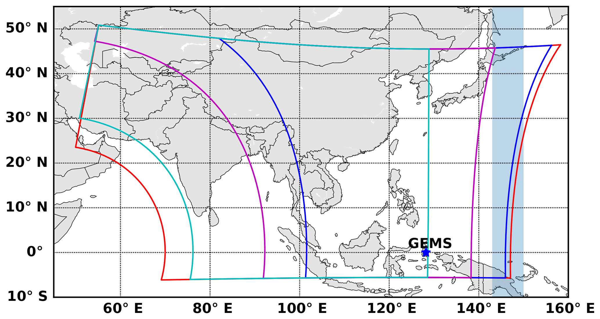
Figure 1GEMS field of regard (red), nominal daily scan (blue), full central scan (magenta), full western scan (cyan), and GEMS location (blue star). Shaded areas (143–150∘ E) are regions for radiance references and common mode.
Table 1Summary of GEMS system attributes, parameters for radiance fitting, and parameters for the air mass factor (AMF) lookup table.
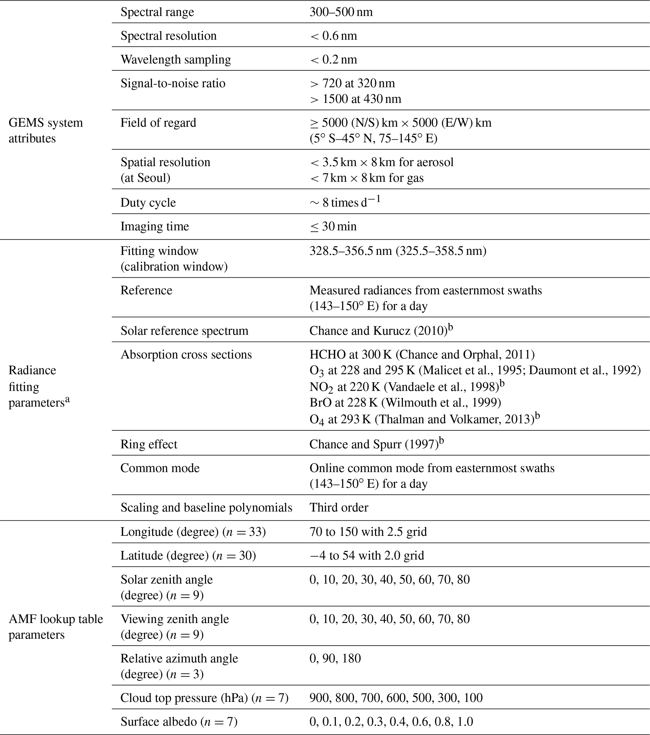
a GEMS fitting parameters follow González Abad et al. (2015). However, undersampling is not included in the fitting parameters for GEMS, and the reference sector for radiance reference and common mode is different. b Datasets used in QA4ECV retrievals. Please refer to De Smedt et al. (2018) for details on other datasets and fitting options.
2.2 HCHO algorithm description
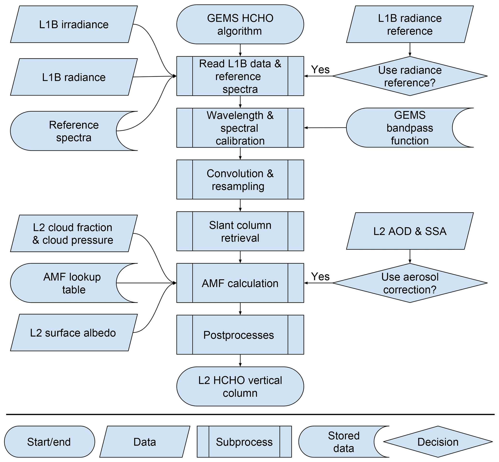
Figure 2 is a flow chart of the HCHO retrieval algorithm for GEMS. The retrieval procedure consists of three steps: preprocesses, radiance fitting, and postprocesses. The preprocesses begin with a wavelength calibration of Level 1B data (irradiance and radiance), as well as interpolation and convolution of absorption cross sections at calibrated wavelength grid points. Radiance fitting is then conducted to derive the HCHO slant columns using a nonlinear least-squares method. Finally, the postprocesses include an air mass factor (AMF) calculation that employs a lookup table to convert HCHO slant columns to vertical columns, an assignment of data quality flags for each pixel, the removal of a possible stripe pattern along each cross-track position, and corrections for background values. Each retrieval step is described in more detail in the following sections.
2.2.1 Wavelength calibration and GEMS bandpass function
Wavelength grid points of measured irradiances and radiances in a charge-coupled-device (CCD) sensor are often shifted or squeezed, and such systematic biases due to wavelength shifts or squeezes need to be corrected when producing Level 1B data. However, as precise wavelength alignments between irradiances/radiances and absorption cross sections are required to achieve accurate radiance fitting, it is also necessary to conduct wavelength calibration during retrieval.
In wavelength calibration, the solar reference spectrum (Chance and Kurucz, 2010) is firstly convolved with a GEMS bandpass function and is then interpolated to the wavelength grids of the measured spectrum. A convolved solar reference spectrum with wavelength shift parameters and polynomial parameters (Eq. 1) is then fitted to the measured irradiances and radiances in a broader fitting window (325.5–358.5 nm) than that of the radiance fitting for HCHO retrievals as follows:
where IR(λ) is the modeled irradiance and radiance, is the solar reference spectrum with a high spectral resolution of 0.01 nm wavelength interval, Δλ is the wavelength shift, g(λ) is a bandpass function, and Psc(λ) and Pbl(λ) are scaling and baseline polynomials, respectively. The symbol ⊗ denotes the convolution procedure, as shown in Eq. (2).
We use the GEMS bandpass functions for the convolution in wavelength calibration to ensure consistency with the spectral resolutions of measured irradiances and radiances. GEMS bandpass functions are provided at seven center wavelengths ranging from −1.8 to 1.8 nm at center wavelengths, with wavelength sampling intervals of 0.06 nm (Fig. 3). Figure 3b shows bandpass functions averaged for spatial indices at 330 and 365 nm, and it also shows the relative differences between bandpass functions at 365 and 330 nm. The relative differences are smaller near the wavelength center, but they increase over each wing of the function. For GEMS HCHO retrieval, we will conduct calibration for every spatial pixel of the sensor using the bandpass functions at 330 nm. However, as bandpass functions are not linear with wavelengths, it will be necessary to estimate uncertainties for the wavelength dependency of the bandpass functions after GEMS is launched.
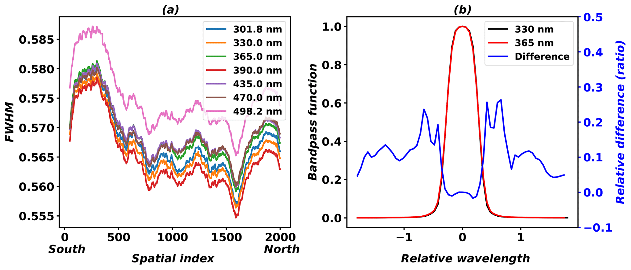
Figure 3Full width at half maximum (FWHM) of GEMS bandpass as a function of spatial index of GEMS detection rows (a) and averaged bandpass functions for spatial indices at 330 and 365 nm and relative differences (b).
2.2.2 Convolution and reference spectra sampling
Table 1 shows a summary of absorption cross-section datasets used in GEMS HCHO retrieval. In the retrieval algorithm, absorption cross-section data with fine spectral resolutions (for example, HCHO absorption cross-section data with a spectral resolution of 0.011 nm) are first convoluted with the bandpass functions described in Sect. 2.2.1, and they are then interpolated to the calibrated wavelength grids of measured radiances. Finally, radiance fitting accounts for attenuation of a reference spectrum (measured irradiance or radiance) by gas absorption using Eq. (3) with convoluted cross-section data as follows:
where τh is the optical depth of interfering gases with fine spectral resolutions.
However, radiative transfer in the atmosphere occurs in a slightly different manner. Solar irradiance is firstly reduced by the absorption of interfering gases, and radiances are subsequently measured on discrete wavelength grids of an instrument with predetermined spectral resolutions, as shown in Eq. (4),
Therefore, the difference between measured and calculated radiances on discrete grids may provide biases in radiance fitting when sensors have limited spectral resolutions, which is referred to as the solar I0 effect (Aliwell et al., 2002; Chan Miller et al., 2014).
We calculate pseudo absorption cross sections to account for the differences in gas absorptions between reality and radiance fitting. We assume that the absorption process in radiance fitting is the same as that in reality, and the pseudo absorption cross sections are computed using the following equation (Aliwell et al., 2002; Chan Miller et al., 2014),
where σps(λ) is a pseudo absorption cross section, scdref is a reference slant column density, and σh(λ) is an absorption cross section with a fine spectral resolution.
Although the corrected absorption cross section can be applied to all the species, we only apply the correction to the O3 absorption cross section, which is the most important interfering species in the fitting window of HCHO retrievals, and we use an O3 reference slant column density of 300 DU for the correction.
2.2.3 Radiance fitting
Three different methods have been used with sun-synchronous satellite measurements in previous HCHO retrievals: the differential optical absorption spectroscopy (DOAS) method (De Smedt et al., 2008, 2012); a nonlinearized fitting method, which is known as basic optical absorption spectroscopy (BOAS) (Chance et al., 2000; González Abad et al., 2015, 2016); and principal component analysis (Li et al., 2015). Zhu et al. (2016) conducted an intercomparison of HCHO vertical column densities retrieved using the three retrieval methods for four instruments such as OMI, GOME-2A, GOME-2B, and OMPS; they found that the different retrieval results were consistent in terms of temporal and spatial variations of HCHO columns in the southeastern United States.
To yield HCHO slant columns in this study, we use the BOAS method, which is based on a nonlinearized form of the Lambert–Beer law, as shown in Eq. (6) (González Abad et al., 2015). One advantage of the BOAS method is that it uses unprocessed radiance data, and it is thus more intuitive than the widely used DOAS method, which uses a linearized form by taking the logarithm of radiance to irradiance and high-pass filtering the result. The modeled radiative equation is given as follows:
where a is an amplitude factor; I0(λ) is a reference spectrum (solar irradiance or radiance reference); crσr(λ) is the contribution of the Ring effect; is the contributions of all gas absorptions; SCDi and σi(λ) are slant column densities and absorption cross sections for species i, respectively; ccmσcm(λ) is the contribution of the common mode; and Psc(λ) and Pbl(λ) are scaling and baseline polynomials, respectively, considering low frequency variations due to Rayleigh and Mie scattering. Furthermore, the modeled spectrum is fitted to measured radiances using a nonlinear least-squares method (Wedin and Lindström, 1987) to yield HCHO slant columns.
The common mode denotes fitting residuals caused by instrument properties which have not been determined from physical analysis. Accounting for the common mode can reduce fitting residuals and fitting uncertainties without affecting the retrieved slant columns (González Abad et al., 2015). The common mode for GEMS can be calculated by averaging fitting residuals at every cross track over easternmost swaths (143–150∘ E) shown as shaded areas in Fig. 1, which are relatively clean regions.
Table 1 summarizes the detailed information used in the GEMS HCHO retrieval algorithm. Fitting options in González Abad et al. (2015) are followed. We use measured radiances as the reference spectrum, called a radiance reference, and measured radiances are averaged over the easternmost swaths (143–150∘ E; shaded areas in Fig. 1) for a day as a function of cross-track positions in the south-to-north direction. Background corrections are required when we use a radiance reference and are discussed in Sect. 2.2.5. Also, GEMS has cross-track swaths in the south-to-north direction while instruments such as OMI and TROPOMI have a west-to-east swath. Therefore, latitudinal biases resulting from BrO and O3 latitude-dependent interferences can be minimized for GEMS and are discussed in Sect. 4.1.
2.2.4 Air mass factor
HCHO slant column densities (Ωs) from the radiance fitting are then converted to vertical columns (Ωv) with an AMF (Eq. 7), which is a correction factor for the light slant path to the vertical path. Previous studies have shown that AMF uncertainty is one of the crucial factors causing retrieval uncertainties (De Smedt et al., 2012, 2018), and AMF uncertainties contribute to retrieval uncertainties by multiple factors including cloud top pressure, cloud fraction, HCHO vertical distribution, aerosol vertical distribution, and aerosol optical properties (Millet et al., 2006; Chimot et al., 2016; Kwon et al., 2017; Hewson et al., 2015).
An AMF can be decoupled with a scattering weight (wl) and a vertical shape factor (Sl) of the target species (Eq. 8), which represent radiative sensitivity to the optical depth of the absorber and a partial column density profile normalized by total vertical column density, respectively, at each layer l () (Palmer et al., 2001). Scattering weights are dependent on the solar zenith angle (θs), viewing zenith angle (θv), relative azimuth angle (θr), surface albedo (αs), cloud top pressure (pcld), and effective cloud fraction (fc).
Surface albedo, effective cloud fraction, and cloud top pressure are retrieved from GEMS and used in the AMF calculations. GEMS Level 2 surface properties include Lambertian equivalent reflectivity (LER) and the daily bidirectional reflectance distribution function (BRDF) (Lee and Yoo, 2018). GEMS LER products are retrieved as composites of minimum LER values for 15 d every hour with fixed viewing geometry so that geometry-dependent LERs are yielded. The effective cloud fraction and cloud top pressure (effective cloud pressure) are retrieved from GEMS with the assumption of a Lambertian cloud surface (cloud surface albedo =0.8) (Veefkind et al., 2016). GEMS surface reflectivity products are also used for cloud retrievals. In addition, the radiative cloud fraction (frc) will be provided from GEMS Level 2 cloud products and is defined by Eq. (9), where Icld and Iclr are radiances over cloud and cloud-free surfaces, respectively.
In order to consider the presence of clouds in the AMF calculations, scattering weights in the partial cloudy scenes are linearly interpolated as a function of radiative cloud fractions with scattering weights for clear sky (wl, nc) and fully covered cloudy sky (wl, wc) (Eq. 10) (Martin et al., 2002; González Abad et al., 2015). The latter (wl, wc) is calculated as a function of cloud top pressures using the assumption of Lambertian cloud surface with a cloud surface albedo of 0.8.
For AMF calculations, we compile an AMF lookup table (LUT) at 340 nm as a function of the variables described in Eqs. (8)–(10) and Table 1. González Abad et al. (2015) showed that the wavelength dependence of scattering weights in the HCHO fitting window is small. Therefore, we ignore the wavelength dependence and use AMF values for one wavelength. The AMF LUT is calculated using VLIDORT v2.6 (Spurr, 2006) with a priori data including temperature, pressure, and gas profiles (O3, NO2, SO2, and HCHO), which were simulated from a 3-D chemical transport model (GEOS-Chem v9-01-02; Bey et al., 2001) driven by Modern-Era Retrospective Analysis for Research and Applications (MERRA) with 47 vertical levels and a horizontal resolution, for 2014.
However, the horizontal resolution of for HCHO profiles in AMF LUT is much coarser than the GEMS horizontal resolution of 7 km×8 km to discern spatial variations by local source emissions. HCHO profiles in AMF LUT are monthly averaged so that hourly variations are not taken into account. In order to resolve these coarser conditions, we can use HCHO profiles with a finer resolution as a function of time. For example, Kwon et al. (2017) showed that HCHO retrievals using monthly mean hourly AMF values were in better agreement with the model simulations in observation system simulation experiments than those using monthly mean AMF values. Additionally, air quality forecasting data can be used to consider hourly varying HCHO profiles. Further studies are required to examine the dependency of AMF calculations on spatial resolutions and temporal variations of HCHO profiles and its effect on GEMS retrieval.
Figure 4 shows examples of scattering weights and vertical profile shapes from the AMF LUT in June with conditions of a solar zenith angle of 30∘, a viewing zenith angle of 0∘, a relative azimuth angle of 90∘, a surface albedo of 0.1, a cloud top pressure of 800 hPa, and an effective cloud fraction of 0.3 over clean and polluted grids. Clean grids are classified as having a HCHO column density less than 3.0×10¹⁵ molecules cm−2 and a surface pressure higher than 990 hPa, and polluted grids have a HCHO column higher than 1.0×10¹⁶ molecules cm−2 and a surface pressure higher than 990 hPa. In Fig. 4, although scattering weights are not significantly changed, the normalized vertical profile (a vertical shape factor) over a polluted area is larger near the surface compared to a clean area, which results in AMF values of 1.55 and 1.28 over the clean and polluted areas, respectively.
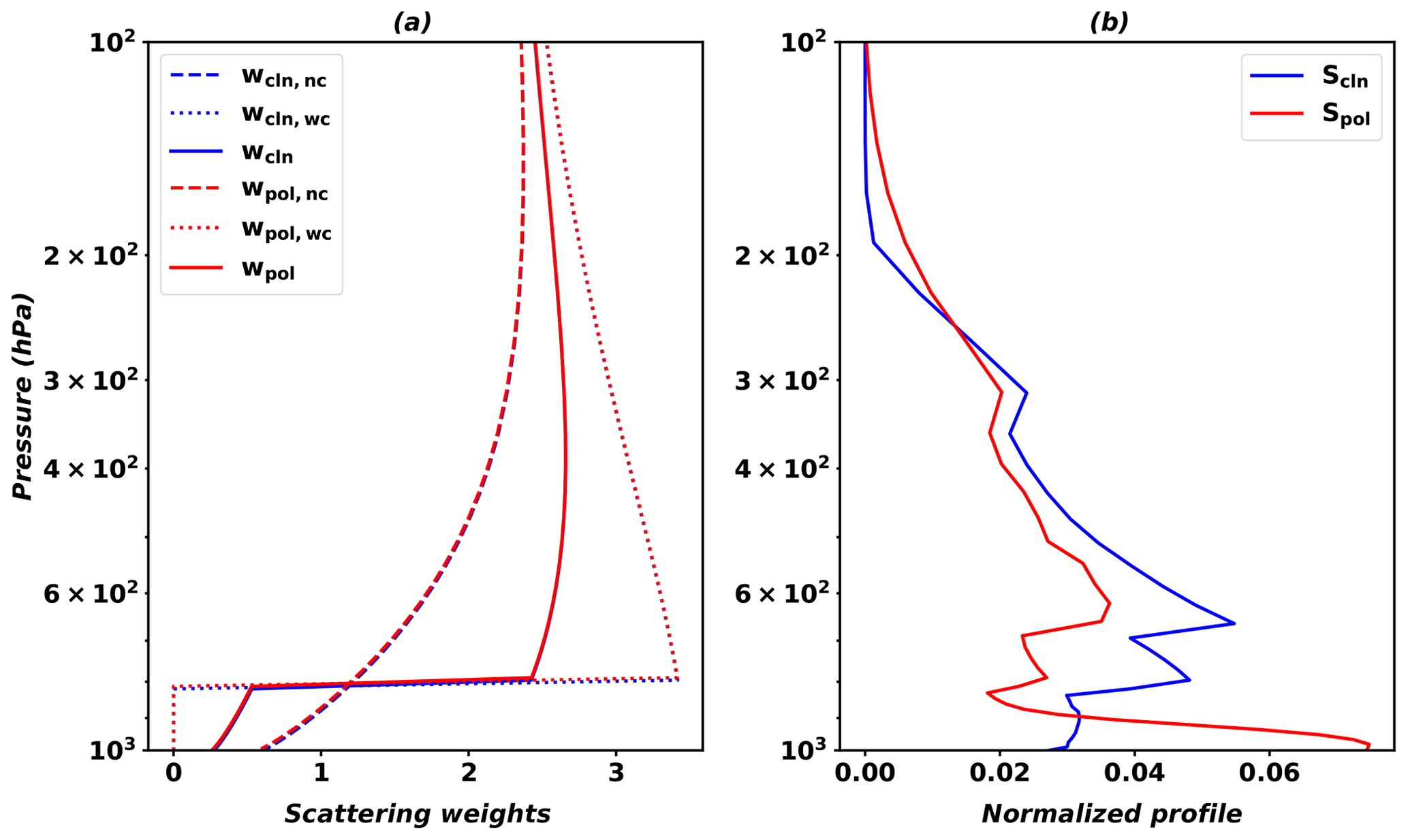
Figure 4Scattering weights (a) and normalized profiles (b) from the AMF LUT over clean (blue) and polluted (red) grids. Dashed and dotted lines in (a) indicate scattering weights with no cloud (nc) and with cloud (wc), respectively. The solid line in (a) indicates scattering weights for a partial cloudy scene calculated using Eq. (10).
2.2.5 Postprocesses
Postprocesses include systematic bias corrections and a statistic data quality flag calculation for each pixel. Systematic bias corrections include cross-track bias correction and background HCHO column correction. Cross-track biases can appear in two-dimensional CCD sensors such as GEMS as functions of each cross-track position when a solar irradiance is used as a reference spectrum (Chan Miller et al., 2014; Nowlan et al., 2016). The cross-track biases are attributed to cross-track variability of the measured irradiance. For example, the biases for OMI are constant at different latitudes; therefore, the biases are shown as stripes in the along-track direction. The cross-track biases are estimated by a polynomial fit through medians of HCHO slant columns for each cross-track position in clean sectors, which are the easternmost swaths for GEMS. The biases are removed from all data measured on the same day for each cross-track position.
An alternative method to avoid the abovementioned biases in the fitting procedure is to use measured radiances over a clean background region (referred to as radiance references) as the reference spectrum in radiance fitting. As measured radiance includes instrument noise and attenuation by interfering gases in the background atmosphere, the interfering effects can be minimized in radiance fitting, which results in negligible cross-track biases.
The retrieved slant columns using a radiance reference are differential slant columns () and do not include background HCHO columns (SCD0) that are mainly from the oxidation of methane. Therefore, the background columns need to be corrected, and we use simulated HCHO vertical columns for 2014 from GEOS-Chem with a spatial resolution of over the reference sector, which is the easternmost regions (143–150∘ E) and is shown as shaded areas in Fig. 1. Simulated HCHO vertical columns are averaged zonally and monthly over the reference sector and are interpolated to 720 latitudinal grid points with a resolution of 0.25∘ from 90∘ S to 90∘ N.
In order to account for dependency of measured radiances on geometric angles, we convert simulated background vertical columns into slant columns by applying AMF values over the reference sector (AMF0), which are calculated with cloud information and geometric angles on the reference sector. Corrected GEMS HCHO slant columns are formulated as the sum of the retrieved differential slant columns and the simulated background slant columns as shown in Eq. (11),
where i and j indicate pixel indices of cross and along tracks, respectively, and VCDm denotes a background vertical column density from the model. We finally apply AMF values from the LUT to the corrected slant columns to obtain GEMS HCHO vertical column densities.
For GEMS, radiance references can be obtained from easternmost swaths, including part of islands near the Equator and Japan, which are relatively clean areas in the south–north direction over the GEMS domain. In comparison with background HCHO vertical columns over the Pacific Ocean for OMI (Fig. S1 in the Supplement), the annual mean of GEMS background columns over 4∘ S–45∘ N is 3.3×10¹⁵ molecules cm−2, which is slightly higher than that of OMI background columns (3.2×10¹⁵ molecules cm−2), showing that we can use the easternmost regions as background in the GEMS domain. Occasionally, local differences between GEMS and OMI background columns can be as large as 3.8×10¹⁵ molecules cm−2 in the tropical region of the Southern Hemisphere due to biogenic activity and biomass burning, but the standard deviation of background values in that region is 5.1×10¹⁴ molecules cm−2, which is even lower than that of 1.2×10¹⁵ molecules cm−2 in the middle latitude (>30∘ N).
After the correction of systematic biases and conversion to vertical column densities with AMFs, all pixels are flagged with vertical columns and fitting uncertainties (González Abad et al., 2015). We assign a data quality flag of 0 for good pixels, where retrieved vertical columns plus two-times fitting uncertainties are positive. The pixels in which retrieved vertical columns are negative within two-times fitting uncertainties, but positive within three-times fitting uncertainties, are assigned with a data quality flag of 1, which represents suspected quality pixels. Pixels with negative vertical columns within three-times fitting uncertainties are designated as bad quality pixels and given a data quality flag of 2, and missing values are flagged by −1. It is of note that these conditions are generous and that tighter conditions for good data may be required for analysis.
We use error and uncertainty terminology from the Guide to the Expression of Uncertainties in Measurements (GUM) (https://www.bipm.org/utils/common/documents/jcgm /JCGM_100_2008_E.pdf, last access: 20 June 2019). Following GUM, “error” means the difference between a measurement result and a true value, and “uncertainty” means the dispersion of measurement values, such as a standard deviation and a full width at half maximum. Because there is a lack of true values for HCHO vertical columns, we consider that the word “uncertainty” is more appropriate for use in our analysis.
Uncertainties in the retrieval steps mentioned in Sect. 2.2 are assumed to be uncorrelated, because the steps are independently performed. Total uncertainty in HCHO vertical column density (VCD) using a radiance reference can be formulated as follows (Boersma et al., 2004; De Smedt et al., 2008):
where σ is the uncertainty in each part; Ωv is the vertical column density; and subscripts v, s, and m represent vertical, slant, and model, respectively. The total uncertainty equation is transformed using Eqs. (7), (11), and (12) into Eq. (13),
We analyze expected uncertainties for the GEMS algorithm by using simulated radiances from Kwon et al. (2017) and OMI Level 1B data. In order to estimate the expected random uncertainty for GEMS (Sect. 3.1.1), we use simulated radiances which are convoluted with GEMS bandpass functions at 330 nm as a function of cross-track positions in the south-to-north direction. Simulated radiances include noises based on the expected signal-to-noise ratio for coadded pixels with spatial resolutions of 7 km×8 km. We use absorption cross sections of the Ring effect, O3, NO2, HCHO, and additionally SO2 (Hermans et al., 2009; Vandaele et al., 2009) in radiance fitting because O3, NO2, and HCHO, and SO2 were considered in the radiance calculation (Kwon et al., 2017).
For other uncertainty analyses, we use OMI Level 1B data with OMI slit function data (Dirksen et al., 2006) in order to examine algorithm sensitivities to different parameters. Fitting options such as absorption cross-section data and the fitting window are summarized in Table 1. It will be necessary to conduct an additional uncertainty analysis for GEMS HCHO retrievals after GEMS is launched.
3.1 Uncertainties in slant columns
3.1.1 Random uncertainty
Uncertainties in slant columns result from random uncertainties (σrand) and systematic uncertainties (σsys) (Eq. 14) (De Smedt et al., 2018),
Random uncertainties are fitting uncertainties when yielding slant columns, and they mainly result from instrument noises. We can reduce random uncertainties by using measured radiances over clean areas as reference spectra instead of irradiances, as the use of measured radiances can minimize instrument noises and interference of O3 and BrO in the stratosphere. In addition, averaging the resulting slant columns for individual pixels can reduce random uncertainties, but this is achieved at the expense of a loss of temporal and spatial resolution (De Smedt et al., 2018).
Random uncertainties can be calculated from root-mean-square (rms) values of fitting residuals, degrees of freedom (m−n), and diagonal components of a covariance matrix (Cj, j) for fitting parameters,
where m and n are the number of spectral grids and fitting parameters, respectively, and j denotes specific species in fitting parameters.
Random uncertainties from the GEMS algorithm are estimated using simulated radiances. The rms values of fitting residuals and random uncertainty for the GEMS domain range from to and 2.1×10¹⁵ to 1.6×10¹⁶ molecules cm−2, respectively, which are comparable with those (rms: to ; random uncertainty: 3.3×10¹⁵ to 1.8×10¹⁶ molecules cm−2) obtained from the GEMS algorithm using OMI Level 1B data. GEMS measures target species every hour in daytime, and changes of solar location during the day can affect the accuracy of radiance fitting. An averaged fitting rms value and a random uncertainty are and 5.0×10¹⁵ molecules cm−2 for conditions with both solar and viewing zenith angles less than 70, which happen at 08:00–18:00 and 09:00–16:00 LT of Seoul in summer and winter, respectively. However, the fitting rms value and the random uncertainty increase to and 8.2×10¹⁵ molecules cm−2, respectively, when solar and viewing zenith angles are higher than 70.
3.1.2 Systematic uncertainty
Systematic uncertainties result from uncertainties of wavelength calibration, the bandpass function for convolution, and absorption cross sections. We estimate systematic uncertainties from sensitivity tests to parameters using OMI Level 1B data. First, systematic uncertainties associated with absorption cross sections are estimated using alternative absorption cross sections: we compare resulting slant columns to the baseline calculation with conditions in Table 1 for a 1-month period (March 2005). In the analysis, we define an uncertainty as a standard deviation of differences between the sensitivity and baseline calculations. Absorption cross sections are convoluted and interpolated using the same spectral resolution and wavelength sampling to enable comparisons between datasets.
To test the retrieval sensitivity to HCHO absorption cross sections, we use HCHO absorption cross-section datasets from Cantrell et al. (1990) instead of those of Chance and Orphal (2011), which provide a rescaling of the datasets in Cantrell et al. (1990) to those of Meller and Moortgat (2000). Absorption cross sections of Cantrell et al. (1990) are ∼10 % lower than those of Chance and Orphal (2011), and the differences are directly linked to slant column retrieval (Pinardi et al., 2013). Therefore, slant columns using Cantrell et al. (1990) are a factor of 1.1 higher than those of the baseline calculation. The slant column changes are similar to values from previous studies (Pinardi et al., 2013; De Smedt et al., 2018).
We conduct a sensitivity test to O3 absorption cross sections at 223 and 293 K from Chehade et al. (2013). Uncertainties of these datasets at both temperatures are ∼4 % in the fitting window of the GEMS algorithm. Compared to the baseline calculation, use of the O3 datasets of Chehade et al. (2013) at 223 and 293 K changes the slant columns by ∼20 % and ∼8 % on average, respectively, which provides uncertainties in slant columns of 1.4×10¹⁵ and 0.57×10¹⁵ molecules cm−2. These uncertainties are larger than those of 13 % and 5 % from Pinardi et al. (2013) and De Smedt et al. (2018), respectively. It thus appears that the GEMS HCHO retrieval algorithm is the most sensitive to O3 absorption, especially at low temperatures in the stratosphere, due to strong absorption in the ultraviolet.
A sensitivity test is conducted against the BrO dataset of Fleischmann et al. (2004), which is ∼9 % lower than the baseline BrO dataset in the GEMS HCHO fitting window and results in ∼4 % slant column changes compared to the baseline calculation (with an uncertainty of 0.28×10¹⁵ molecules cm−2).
We then examine slant column uncertainties for O4 and NO2 absorption cross sections. We use alternative O4 absorption cross sections from http://spectrolab.aeronomie.be/o2.htm (last access: 20 June 2019) that have differences of 28 % compared to the dataset used in the baseline calculation. Due to the large uncertainties of the data compared to other absorption cross-section data, the resulting slant column changes are significant, ∼24 %, with an uncertainty of 1.6×10¹⁵ molecules cm−2. This uncertainty could thus be decreased by reducing the uncertainties of the O4 datasets. Also, O4 should be included in the large fitting interval for HCHO because it has strong peaks near 344.0 and 361 nm (De Smedt et al., 2015; Thalman and Volkamer, 2013). The NO2 datasets from Burrows et al. (1998) are 2 % larger than those in the baseline calculation; switching to them leads to ∼5 % slant column changes with uncertainty of 0.37×10¹⁵ molecules cm−2.
We also estimate the systematic uncertainties of slant columns for wavelength calibration and solar I0 effects by using an alternative solar irradiance reference. As described in Sect. 2.2.1 and 2.2.2, a solar irradiance reference spectrum was used in the wavelength calibration and calculation of pseudo absorption cross sections related to the solar I0 effect. An alternative reference spectrum from the Kitt Peak National Observatory (Kurucz et al., 1984) is almost identical to that of the baseline calculation, but the resulting slant column changes are up to ∼14 % with uncertainty of 0.92×10¹⁵ molecules cm−2. We thus consider that the solar I0 effect associated with the strongest interfering gas (O3) is very sensitive to the reference spectrum.
The total systematic uncertainty of slant columns for the parameters discussed is 38 % of the slant column densities on average for 1 month. This uncertainty is larger than that of De Smedt et al. (2018), which is 20 % of the slant column densities. However, there are remaining slant column uncertainties resulting from uncertainties relating to other parameters, such as polynomial orders in Eq. (6), instrument bandpass functions, and temperature dependency of cross sections. Therefore, we estimate the systematic uncertainty as being 38 % of the slant columns, prior to conducting uncertainty analyses on other parameters.
3.2 Uncertainty in AMF
The AMF uncertainty can be estimated by each parameter in Eq. (16). We examine AMF uncertainties for surface albedo (αs), cloud top pressure (pc), and effective cloud fraction (fc) with a solar zenith angle of 30∘, a viewing zenith angle of 30∘, and a relative azimuth angle of 0∘. In addition, we define a profile height parameter (ph) as an altitude below which 75 % of HCHO VCDs exist from the surface to estimate AMF uncertainty with respect to a HCHO profile shape (De Smedt et al., 2018). The uncertainties of parameters (, hPa, and ) are based on De Smedt et al. (2018) and will be replaced to those from GEMS Level 2 products. The uncertainty of profile height () is defined as a standard deviation of profile heights in AMF LUT, and in polluted and clean areas is 84 and 55 hPa, respectively.
Figure 5a shows AMF sensitivities to surface albedos with clear-sky conditions (fc=0). AMF values increase linearly with an increase in surface albedos and are slightly higher for clean regions than polluted regions in which HCHO is concentrated near the surface.
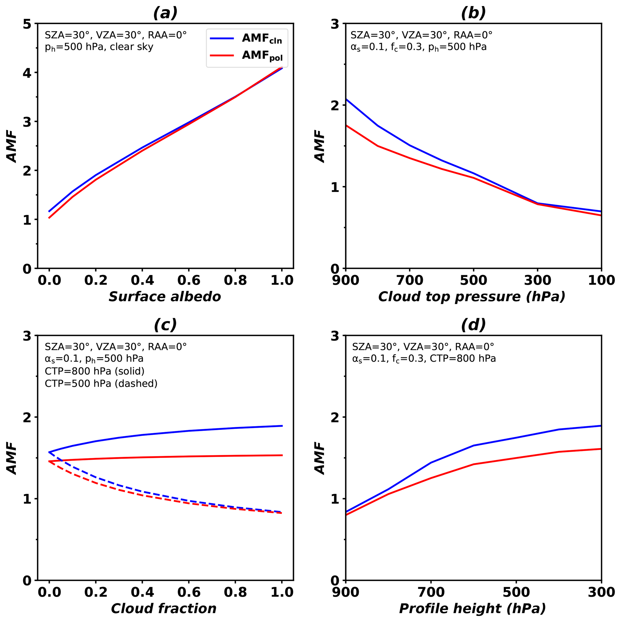
Figure 5AMF variations as functions of (a) surface albedo, (b) cloud top pressure (CTP), (c) effective cloud fraction (fc), and (d) profile height over clean (blue) and polluted (red) areas. Conditions of the AMF LUT are given in the figures. For sensitivity to surface albedo, cloud-free conditions are assumed. For sensitivity to cloud fraction, cloud top pressures are 800 hPa (solid line) and 500 hPa (dashed line).
Clouds below or within HCHO layers increase photon path lengths due to multiple scattering, while clouds at altitudes above HCHO layers shield photons from reaching the surface. Therefore, the AMF values decrease with a decrease in cloud top pressures (with an increase in cloud heights) due to fewer photons reaching the surface (Fig. 5b). AMFs rapidly change with increasing cloud top pressures near the surface, implying a high AMF sensitivity to the changes in photon path lengths with respect to multiple scattering.
Cloud fractions also play an important role in determining AMF values and their effects are shown in Fig. 5c. For a cloud with its top pressure at 800 hPa, AMF values increase with an increase in the cloud fraction, which implies that more photons arrive at the near surface due to multiple scattering by clouds with increasing cloud fractions. However, for clouds with its top pressure at high altitudes (500 hPa), AMF values decrease with an increase in cloud fractions due to the shielding effect of clouds.
Figure 5d shows increasing AMF values with an increase in the profile height, resulting from increased HCHO absorptions at high altitudes. The AMF sensitivity to profile heights in clean areas is higher than that in polluted areas because HCHO distributions are more uniform in clean areas than polluted areas.
Table 2Retrieval uncertainties of GEMS HCHO VCD due to AMF uncertainties as functions of surface albedos, cloud top pressures, cloud fractions, and HCHO profile heights for clean and polluted areas. Values are calculated for conditions with a solar zenith angle of 30∘, a viewing zenith angle of 30∘, a relative azimuth angle of 0∘, cloud fractions less than 0.3, and a profile height of 700 hPa.
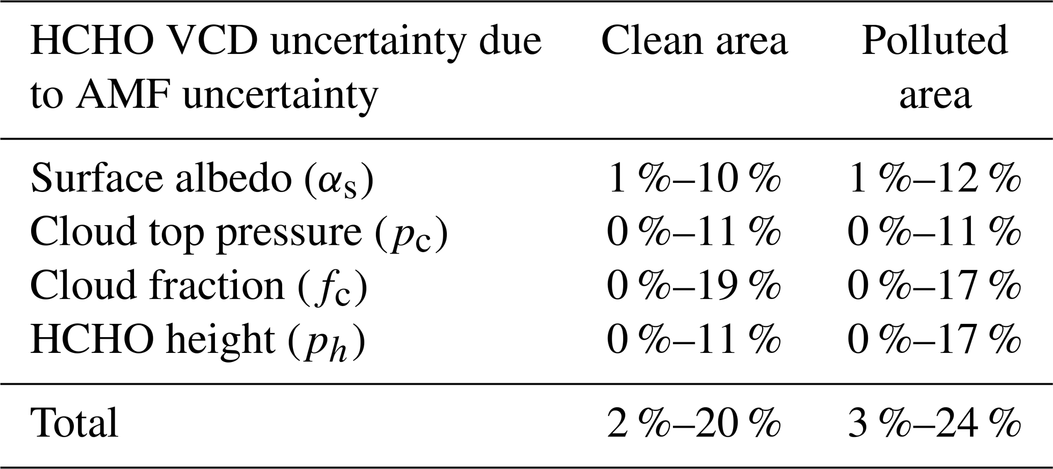
Table 2 summarizes estimated retrieval uncertainties of GEMS HCHO VCDs due to AMF uncertainties as functions of surface albedos, cloud top pressures, and cloud fractions. Values are calculated assuming conditions with solar zenith angle of 30∘, viewing zenith angle of 30∘, relative azimuth angle of 0∘, cloud fractions less than 0.3, and a profile height of 700 hPa. Uncertainties of HCHO VCDs due to AMF uncertainties can be as large as 20 % and 24 % of HCHO VCDs in clean and polluted areas, respectively. Maximum values occur for conditions with low surface albedo, clouds at high altitudes, and high cloud fractions, but they do not differ significantly between clean and polluted areas. However, AMF-driven HCHO uncertainty with respect to the profile height in polluted areas is higher than that in clean areas, implying that accurate HCHO profile information in polluted areas is important for the GEMS HCHO retrieval. We can minimize the a priori HCHO profile uncertainties by using averaging kernels.
Aerosol vertical distributions and aerosol optical properties are also important sources of AMF uncertainty (Chimot et al., 2016; Kwon et al., 2017; Hewson et al., 2013). Nonabsorbing aerosols play a similar role to that of clouds in radiative transfer and are implicitly considered when cloud information is used. However, absorbing aerosols, such as mineral dust and black carbon, counteract the effects of nonabsorbing aerosols and clouds. In the GEMS domain, dust storms and biomass burning occur seasonally, and we may therefore need to consider the effect of absorbing aerosols on the retrieval. We plan to update our AMF LUT as a function of aerosol optical depth, single-scattering albedo, and aerosol height – all of which will be retrieved by GEMS – to account for the effect of absorbing aerosols. Online AMF calculation can also be used for aerosol correction with cloud information and model simulation (Lin et al., 2014).
3.3 Uncertainty in background correction
The uncertainties of model results for background concentrations (σm) and AMFs over the reference sector () are important for background corrections (σbg) in Eq. (17), which represents the third and fourth terms on the right-hand side of Eq. (13),
We estimate model uncertainties by using standard deviations of model results as a function of latitude. Standard deviations range from 2.3×10¹⁴ to 1.4×10¹⁵ molecules cm−2. Uncertainties related to AMF in the reference sector are identical to those discussed in Sect. 3.2.
In this section, we use OMI Level 1B data to validate our retrieval algorithm. Resulting HCHO products are compared with OMI products of other institutes for 1 month of each season (March, June, September, and December) in 2005 to provide seasonal variation in the GEMS domain. We also compared OMI products with ground-based MAX-DOAS at two sites in Europe for 2005 and one site in China for 2016.
4.1 Retrieval of OMI HCHO
GEMS fitting options described in Table 1 are largely consistent with those of OMHCHO products (González Abad et al., 2015). However, we do not include spectral undersampling (Chance et al., 2005) in the fitting process for GEMS, and the reference sector for a radiance reference is 143–150∘ E (shaded areas in Fig. 1). For OMI products, spectral undersampling needs to be included, and radiance references are from the Pacific Ocean as described in González Abad et al. (2015). We use simulated HCHO vertical columns for the background correction, which are zonally and monthly averaged over the reference sector (140–160∘ W, 90∘ S–90∘ N), except for Hawaii (154–160∘ W, 19–22∘ N).
In addition, we need to correct latitudinal biases for OMI. Previous studies explained that the latitudinal biases result from spectral interferences of BrO and O3, whose concentrations are a function of latitude and are high in high latitudes (De Smedt et al., 2008, 2015; González Abad et al., 2015). Therefore, the latitudinal biases were corrected when a radiance reference was used as the reference spectrum (De Smedt et al., 2008, 2018; González Abad et al., 2015). We correct the latitudinal biases, which are slant columns retrieved for a radiance reference and are averaged as a function of latitude, by subtracting the biases from the corrected slant columns in Eq. (11).
Figure 6 shows OMI HCHO slant columns from OMHCHO products (Fig. 6a) and the GEMS algorithm without and with latitudinal bias corrections (Fig. 6b and c). HCHO slant columns without latitudinal bias corrections (Fig. 6b) are retrieved larger in 5–25∘ N than OMHCHO products, but HCHO slant columns with the bias corrections are in better agreement with OMHCHO products. Figure 6d shows the absolute differences between OMI HCHO slant columns with and without latitudinal bias corrections from the GEMS algorithm as latitudinal biases. Slant columns with bias corrections increase at latitudes lower than 5∘ N and higher than 25∘ N but decrease at latitudes from 5 to 25∘ N.

Figure 6HCHO slant column densities (8 March 2005, orbit 3436): (a) OMHCHO products, (b) the GEMS algorithm without latitudinal bias corrections and (c) GEMS with latitudinal bias corrections, and (d) differences (c–b).
However, latitudinal biases can be minimized when using a radiance reference as a function of each cross-track position in the south-to-north direction for GEMS. In default fitting options, therefore, we do not include latitudinal correction and do not analyze uncertainty of latitudinal corrections in Sect. 3. However, a further investigation for the latitudinal biases needs to be required after GEMS is launched.
Figure 7 shows an example of retrieved HCHO optical depths and fitting residuals as functions of wavelengths for a pixel in Indonesia (23 March 2005; orbit 3655). The retrieved HCHO slant column is 3.2×10¹⁶ molecules cm−2, which is relatively high due to biomass burning in that region. Averaged slant column and random uncertainty for all pixels on the orbit are 7.6×10¹⁵ and 6.9×10¹⁵ molecules cm−2, respectively, over the GEMS domain. The large random uncertainty of 100 % or larger results from pixels with low concentrations, where averaged slant columns and random uncertainties are 2.2×10¹⁵ and 6.2×10¹⁵ molecules cm−2.
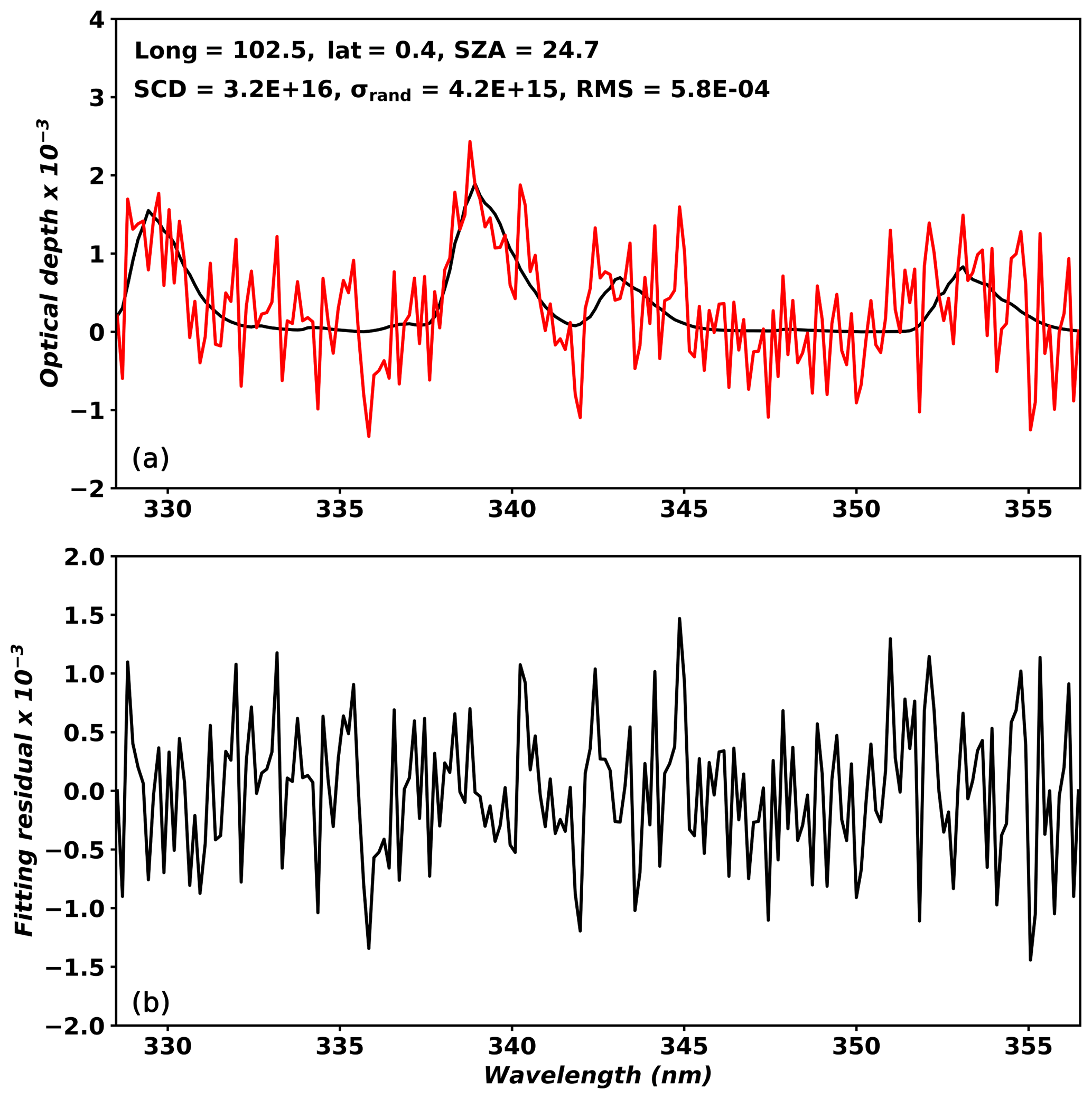
Figure 7Fitted HCHO optical depth (a) and fitting residuals (b) on a pixel (23 March 2005; orbit 3655) with a main data quality flag of 0 and an effective cloud fraction less than 0.3. In (a), the black solid line indicates optical depth, and the red solid line indicates HCHO optical depth plus fitting residuals.
4.2 Comparison with other OMI products
Figure 8 compares monthly mean slant columns retrieved using the GEMS algorithm and those of OMHCHO products (González Abad et al., 2015). We select pixels with (1) vertical columns ranging from to 10×1016 molecules cm−2, (2) a main data quality flag of 0, (3) an effective cloud fraction of less than 0.3, and (4) a solar zenith angle of less than 60. Monthly mean slant column densities are weighted by uncertainties and overlapped areas between pixels and grid boxes with a horizontal resolution of .
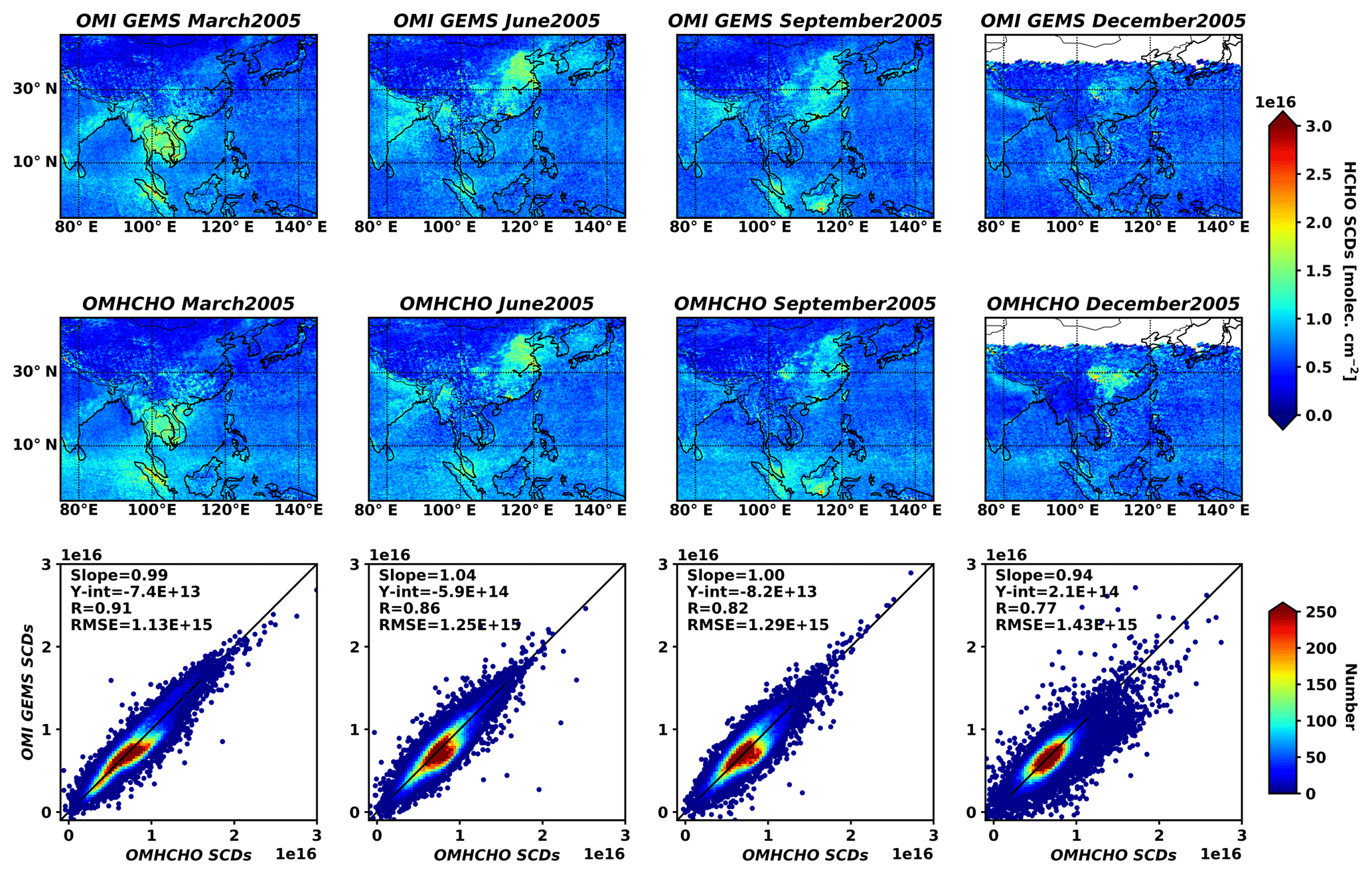
Figure 8Monthly mean slant column densities (SCDs) from the GEMS algorithm (first row) and OMHCHO products (second row) for 4 months in 2005, and scatter plots between GEMS and OMHCHO. Statistics are given in the figures.
We find similar spatial patterns of HCHO slant columns in both products; this shows that high HCHO columns occur over Indonesia and the Indochina Peninsula in March and over Indonesia in September, owing to biomass burning and biogenic activities. In summer, HCHO enhancements over China are caused by biomass burning and the oxidation of biogenic and anthropogenic VOCs due to photochemical reactions. In addition, high HCHO slant column densities occur over the Pearl River Delta, where anthropogenic VOCs are emitted from petrochemical industries, cargo ports, paint production, and many other activities (Zhong et al., 2013). The scatter-plot comparisons with OMHCHO products show that GEMS HCHO slant columns are in good agreement with OMHCHO products, with correlation coefficients of 0.77–0.91 and regression slopes of 0.94–1.04. The relative differences between GEMS slant columns and those of OMHCHO products are −3 % to 0.1 % on average over the domain.
However, some discrepancies are found despite overall good agreement between GEMS and OMHCHO products, and these are mainly related to the background correction from the different model results. Figure 9 shows the simulated HCHO vertical columns used for background corrections in OMHCHO (solid lines) and the GEMS algorithm (dashed lines), respectively. Similar latitudinal variations are shown with a peak in the tropics and gradual decreases in high latitudes, which reflects the photochemical production of HCHO; however, the magnitudes slightly differ. The model results used in GEMS are smaller than those used in the OMHCHO products (especially within ±20∘ latitudes) by molecules cm−2 near 6∘ N in September. Both results were obtained from the same 3-D global chemical transport model (GEOS-Chem), but different assimilated meteorological products were employed. HCHO vertical columns used in the OMHCHO products were from GEOS-Chem with GEOS-4 meteorological data (Millet et al., 2006), which have lower cloud optical depths near the Equator compared to GEOS-3 and GEOS-5. Therefore, low cloud optical depths in the tropics resulted in faster methane oxidation and the production of more HCHO in relation to high hydroxyl radical concentrations (http://wiki.seas.harvard.edu/geos-chem/index.php/GMAO_GEOS-4, last access: 20 June 2019). González Abad et al. (2016) also showed that the OMHCHO products are larger than OMI BIRA-IASB products near the Equator, such as in southeastern Asia, tropical Africa, and the Amazon basin.
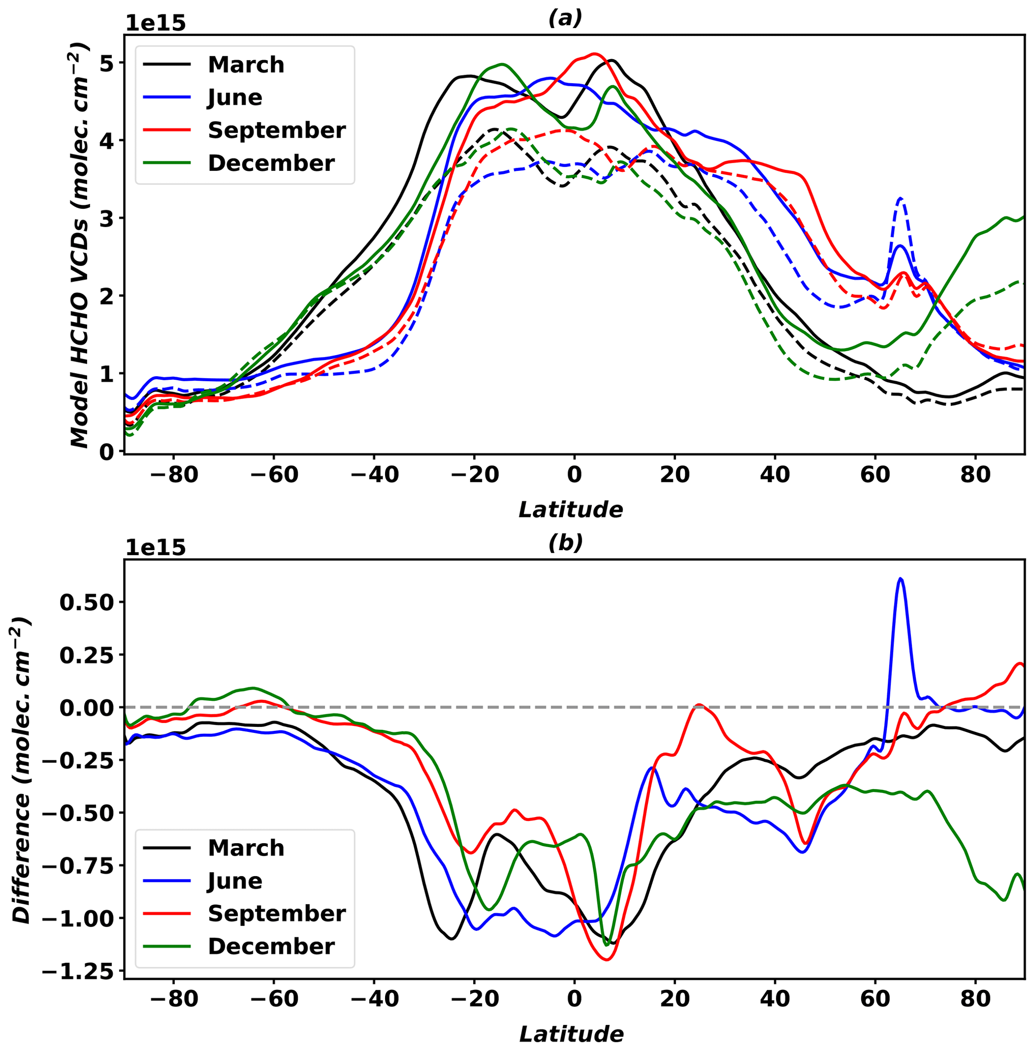
Figure 9Simulated HCHO vertical column densities used in OMHCHO (solid lines) and the GEMS algorithm (dashed lines) for background correction (a), and absolute differences of model results between the GEMS algorithm and OMHCHO (b).

Figure 10Monthly mean slant column densities (SCDs) from the GEMS algorithm (first row) and OMI QA4ECV products (second row) for 4 months in 2005, and scatter plots between GEMS and OMI QA4ECV. Statistics are given in the figures.
We select four regions (Sumatra/Malaysia, the Indochina Peninsula, China, and Borneo), where HCHO is abundant from biomass burning and biogenic and anthropogenic sources. Table 3 provides the relative differences between OMI GEMS HCHO slant columns and OMHCHO slant columns in these four regions. GEMS HCHO slant columns are 1 % to 13 % lower than those of OMHCHO in Sumatra/Malaysia and Borneo, because the differences in simulated HCHO column densities for background corrections are relatively large near the Equator compared to the midlatitudes, as previously mentioned. In the Indochina Peninsula and China, however, the GEMS HCHO slant columns are 6 % to 25 % higher than the OMHCHO slant columns, although the simulated HCHO concentrations used in the GEMS algorithm for background corrections are lower than those used in OMHCHO.
Table 3Relative differences between OMI GEMS HCHO slant columns and OMHCHO and OMI QA4ECV slant columns in four regions.
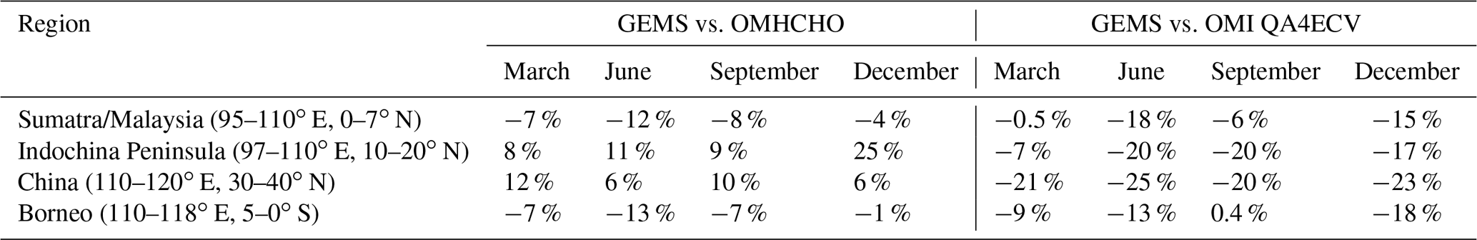
We also compare OMI GEMS HCHO slant columns with OMI QA4ECV products (OMI QA4ECV) (De Smedt et al., 2018). The QA4ECV project was proposed to provide reliable satellite and ground-based measurements of climate and air quality variables with detailed uncertainty information (http://www.qa4ecv.eu, last access: 20 June 2019). Figure 10 shows that the spatial distributions of the GEMS HCHO slant columns are consistent with those of the OMI QA4ECV products, but relatively poorer correlation coefficients of 0.52 to 0.76 are found compared to those with the OMHCHO products. The relative differences between GEMS and QA4ECV slant columns range from −11 % to −22 % on average over the GEMS domain.
Magnitudes of relative differences between OMI GEMS and OMI QA4ECV slant columns vary regionally and seasonally (Table 3). The differences are relatively small near the Equator (Sumatra/Malaysia and Borneo) compared to those in subtropics and midlatitudes (Indochina Peninsula and China) because biomass burning often occurs and biogenic sources are more abundant near the Equator. The HCHO differences near the Equator are lower in spring and fall than those in summer and winter due to biomass burning. The effects of biomass burning on HCHO slant columns are also found over the Indochina Peninsula in spring. As a result, magnitudes of relative differences in regions and seasons with high HCHO concentrations are small, implying that HCHO can be well-retrieved because of the abundant HCHO concentrations, regardless of the fitting method used.
The discrepancy between the two products could result from the radiance fitting. The OMI QA4ECV products use the DOAS method while the GEMS algorithm uses a nonlinearized fitting method (BOAS) for radiance fitting. We also find that polynomial orders accounting for Rayleigh and Mie scatterings are important factors, causing differences between the two products. Retrieved slant columns using the fourth polynomial order are in better agreement with the QA4ECV products (Fig. S2). Both correlation coefficient and regression slope are improved although OMI GEMS HCHO values are higher than those of the QA4ECV. We use the fourth-order polynomial instead of the fifth-order one used in the QA4ECV products because slant columns retrieved using the fifth-order one in the GEMS algorithms are much higher than the QA4ECV products.
Also, different O3 absorption cross sections (Serdyuchenko et al., 2014) are used in the OMI QA4ECV at different temperatures (220 and 243 K), and a nonlinear O3 absorption effect (Puķīte et al., 2010) is included in the OMI QA4ECV. We examine the O3 effects on retrieved slant columns in the GEMS algorithm using O3 datasets used in QA4ECV and considering a nonlinear O3 absorption effect. Correlation coefficient and regression slopes are slightly improved (Table S1 in the Supplement), and relative differences in the four regions defined above are slightly reduced in most seasons and regions (Table S2).
4.3 Comparison with ground-based MAX-DOAS
We also compare satellite results with MAX-DOAS ground observations at Haute-Provence Observatory (OHP) in France, Bremen in Germany, and Xianghe in China (Table 4). MAX-DOAS data are collected within the OMI overpass time (12:00–15:00 LT) at OHP and Bremen in 2005 and at Xianghe in 2016. We collect OMI data pixels that are overlapped by a grid box of 0.25∘ at the center of the site location, and average values of OMI data are weighted by uncertainties and overlapped areas between pixels and grid boxes.
Table 4Averaged HCHO VCDs (molecules cm−2) from MAX-DOAS ground observations and OMI satellite data at OHP in France, Bremen in Germany, and Xianghe in China. For satellites, mean values are weighted by uncertainties and overlapped areas between satellite pixels and 0.25∘ grid cells for each site. Relative differences between OMI and MAX-DOAS are given in parentheses.
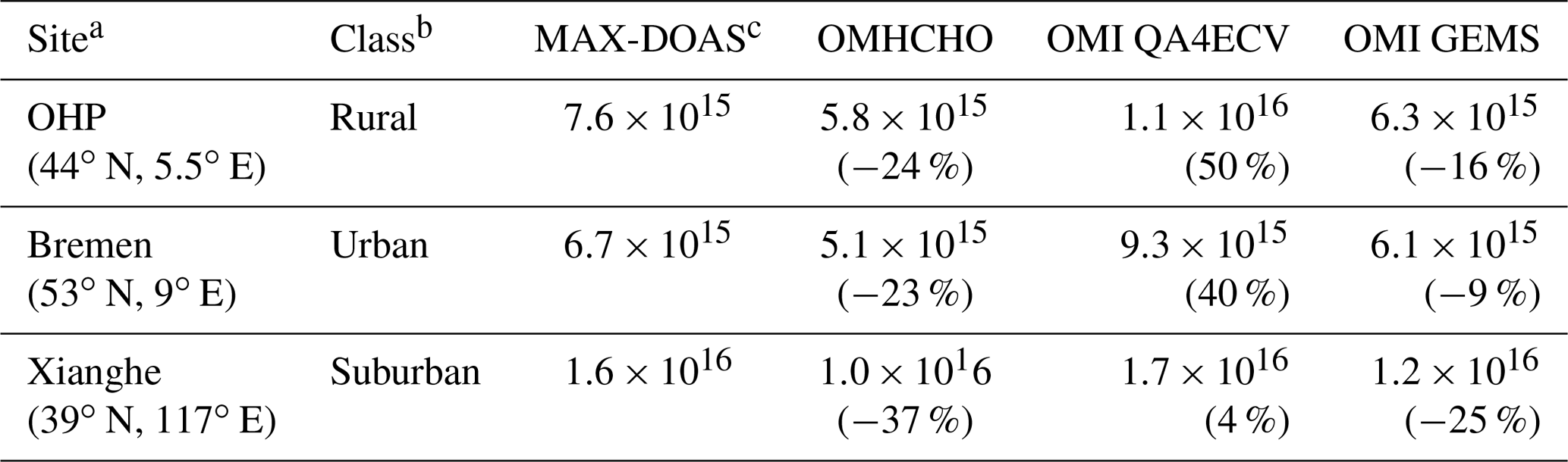
a HCHO VCDs are averaged at OHP and Bremen in 2005 and at Xianghe in 2016. b Class is assigned in a QA4ECV MAXDOAS website (http://uv-vis.aeronomie.be/groundbased/QA4ECV_MAXDOAS, last access: 20 June 2019). c Fitting windows of 336–359 nm are used at OHP and Bremen, and fitting windows of 324–359 nm are used at Xianghe.
Comparisons of HCHO VCDs between MAX-DOAS and satellite products are shown in Fig. 11 and Table 4. Averaged MAX-DOAS HCHO VCDs for a year are 7.6×10¹⁵, 6.7×10¹⁵, and 1.6×10¹⁶ molecules cm−2 at OHP, Bremen, and Xianghe, respectively. HCHO VCDs show a seasonal variation with the maximum concentrations in summer at all sites (Fig. S3). The largest monthly change is shown at Xianghe, likely driven by abundant VOC precursors for HCHO production compared to OHP and Bremen.

Figure 11HCHO vertical columns from MAX-DOAS, OMHCHO, OMI QA4ECV, and OMI GEMS at OHP and Bremen in 2005 and at Xianghe in 2016. Orange lines are median values for each dataset, and blue diamonds are mean values. We computed mean values of each satellite product weighted by uncertainties and overlapped areas between satellite pixels and 0.25∘ grid cells for each site. Boundaries of boxes indicate the first and last quantiles of datasets.
Averaged HCHO VCDs from OMI GEMS are 16 %, 9 %, and 25 % lower than those from MAX-DOAS at OHP, Bremen, and Xianghe. At Bremen, HCHO VCDs from the GEMS algorithm are in the best agreement with those of MAX-DOAS and show similar monthly variations with MAX-DOAS. OMI GEMS results at Xianghe show a monthly variation but do not show a monthly variation at OHP despite a small increment in summer. In particular, the GEMS algorithm yields lower HCHO VCDs in summer. These lower values may be caused by the a priori HCHO profiles used in AMF calculation. In summer, HCHO is produced and concentrated near the surface, which results in lower AMFs (higher VCDs). S. W. Kim et al. (2018) showed the anticorrelation between AMF values and the HCHO mixing ratios at 200 m above ground level. OMHCHO products show similar tendencies to OMI GEMS, but they are much lower than those of OMI GEMS. OMI QA4ECV products are higher than MAX-DOAS at OHP and Bremen but are in the best agreement with MAX-DOAS at Xianghe compared to other satellite products.
We have developed a GEMS HCHO algorithm based on a nonlinearized fitting method and described the algorithm in detail. The GEMS HCHO algorithm consists of three steps: preprocesses, radiance fitting, and postprocesses. Preprocesses include wavelength calibration, as well as interpolation and convolution of absorption cross sections. In the radiance fitting, HCHO slant column densities are retrieved by minimizing the difference between calculated radiances with initial guesses of absorbing gases and measured radiances in HCHO fitting windows. Finally, AMF values are calculated from an AMF LUT, and bias corrections are conducted if necessary.
We estimated the uncertainties of slant columns, AMF, and background corrections using simulated radiances and OMI Level 1B data. The random uncertainties of slant columns are estimated using simulated radiances and are comparable with those of OMI GEMS products. The systematic uncertainty is 38 % of the slant columns, which is higher than that of De Smedt et al. (2018). However, the systematic uncertainty can be reduced by using up-to-date absorption cross sections. AMF uncertainty amounts to 20 % and 24 % of the HCHO vertical columns in clean and polluted areas, respectively, and mainly results from uncertainties associated with HCHO profile heights and cloud information (cloud top pressure and cloud fractions).
OMI HCHO columns from the GEMS algorithm were compared to the OMHCHO products with consistent fitting conditions applied. OMI GEMS slant columns show good agreement with OMHCHO products, with correlation coefficients of 0.77–0.91 and regression slopes of 0.94–1.04. However, some differences between two products were found because of background corrections. Both products used the model results simulated by GEOS-Chem but driven with different assimilated meteorological datasets. The simulated HCHO vertical columns used in OMHCHO products were from GEOS-Chem with GEOS-4 meteorological data, which have lower cloud optical depths near the Equator compared to GEOS-3 and GEOS-5. Low cloud optical depths in the tropics result in faster methane oxidation and greater HCHO production caused by high hydroxyl radical concentrations. Therefore, OMHCHO slant columns are 1 % to 13 % higher than OMI GEMS slant columns in Sumatra/Malaysia and Borneo near the Equator.
The spatial distributions of GEMS HCHO slant columns were consistent with OMI QA4ECV products, but relatively poorer correlation coefficients of 0.52 to 0.76 are found compared to those with OMHCHO products. Relative differences between GEMS and QA4ECV slant columns range from −11 % to −22 % on average over the GEMS domain. We found that the discrepancy between the GEMS and QA4ECV products was mainly caused by polynomial orders in the fitting window, the different O3 absorption datasets, and consideration of the nonlinear O3 absorption effect.
We also compared satellite results with MAX-DOAS ground observations at OHP in France, Bremen in Germany, and Xianghe in China. HCHO VCDs from the GEMS algorithm were 16 %, 9 %, and 25 % lower than those of MAX-DOAS, but the GEMS discrepancies at OHP and Bremen were the smallest compared to the other satellites against the in situ data.
After GEMS is launched, several options need to be tested. As described in Sect. 2.2.1, it will be necessary to estimate uncertainties resulting from the wavelength dependence of bandpass functions. We may also need to conduct additional sensitivity tests to optimize the fitting window and fitting options. We currently use a broad fitting window (328.5–356.0 nm). However, we may need to use a different fitting window to reduce interference from polarization effects because GEMS does not include a polarization scrambler. A polarization correction is planned to minimize its interference during GEMS Level 1B production, but we need to examine the retrieval sensitivity to polarization. Additionally, an update to the optimized AMF LUT with finer spatial and temporal resolutions is required.
OMHCHO products are available at https://doi.org/10.5067/Aura/OMI/DATA2015 (Chance, 2007; González Abad et al., 2015). OMI QA4ECV products are available at http://www.qa4ecv.eu/ecv/hcho-p/data (last access: 20 June 2019) (De Smedt et al., 2018). MAX-DOAS data are available at http://uv-vis.aeronomie.be/groundbased/QA4ECV_MAXDOAS/index.php (last access: 20 June 2019).
The supplement related to this article is available online at: https://doi.org/10.5194/amt-12-3551-2019-supplement.
HAK and RJP designed the study, carried out the analyses, and wrote the manuscript. GGA, KC, TPK, and JK participated in algorithm development. IDS and MVR carried out measurements for OMI QA4ECV and MAX-DOAS at OHP and Xianghe. EP and JB carried out MAX-DOAS measurements at Bremen.
The authors declare that they have no conflict of interest.
We thank the anonymous reviewers for their invaluable comments. This subject is supported by the Korea Ministry of Environment (MOE) as the Public Technology Program based on Environmental Policy (2017000160001). Part of the research was carried out at the Jet Propulsion Laboratory, California Institute of Technology, under a contract with NASA. Research at the Smithsonian Astrophysical Observatory was supported by NASA grant NNX13AI43G, SAO Participation in the Korean Geostationary Environment Monitoring Spectrometer (GEMS): Instrument Design and Algorithm Development.
This research has been supported by the Korea Ministry of Environment (MOE) as the Public Technology Program based on Environmental Policy (grant no. 2017000160001).
This paper was edited by Helen Worden and reviewed by three anonymous referees.
Aliwell, S. R., Van Roozendael, M., Johnston, P. V., Richter, A., Wagner, T., Arlander, D. W., Burrows, J. P., Fish, D. J., Jones, R. L., Tørnkvist, K. K., Lambert, J. C., Pfeilsticker, K., and Pundt, I.: Analysis for BrO in zenith-sky spectra: An intercomparison exercise for analysis improvement, J. Geophys. Res., 107, ACH-10-11–ACH-10-20, https://doi.org/10.1029/2001JD000329, 2002.
Barkley, M. P., De Smedt, I., Van Roozendael, M., Kurosu, T. P., Chance, K., Arneth, A., Hagberg, D., Guenther, A., Paulot, F., and Marais, E.: Top-down isoprene emissions over tropical South America inferred from SCIAMACHY and OMI formaldehyde columns, J. Geophys. Res.-Atmos., 118, 6849–6868, https://doi.org/10.1002/jgrd.50552, 2013.
Bey, I., Jacob, D. J., Yantosca, R. M., Logan, J. A., Field, B. D., Fiore, A. M., Li, Q., Liu, H. Y., Mickley, L. J., and Schultz, M. G.: Global modeling of tropospheric chemistry with assimilated meteorology: Model description and evaluation, J. Geophys. Res., 106, 23073–23095, https://doi.org/10.1029/2001JD000807, 2001.
Boersma, K. F., Eskes, H. J., and Brinksma, E. J.: Error analysis for tropospheric NO2 retrieval from space, J. Geophys. Res., 109, D04311, https://doi.org/10.1029/2003JD003962, 2004.
Burrows, J. P., Dehn, A., Deters, B., Himmelmann, S., Richter, A., Voigt, S., and Orphal, J.: ATMOSPHERIC REMOTE-SENSING REFERENCE DATA FROM GOME: PART 1. TEMPERATURE-DEPENDENT ABSORPTION CROSS-SECTIONS OF NO2 IN THE 231–794 nm RANGE, J. Quant. Spectrosc. Ra., 60, 1025–1031, https://doi.org/10.1016/S0022-4073(97)00197-0, 1998.
Cantrell, C. A., Davidson, J. A., McDaniel, A. H., Shetter, R. E., and Calvert, J. G.: Temperature-dependent formaldehyde cross sections in the near-ultraviolet spectral region, J. Phys. Chem., 94, 3902–3908, https://doi.org/10.1021/j100373a008, 1990.
Chan Miller, C., Gonzalez Abad, G., Wang, H., Liu, X., Kurosu, T., Jacob, D. J., and Chance, K.: Glyoxal retrieval from the Ozone Monitoring Instrument, Atmos. Meas. Tech., 7, 3891–3907, https://doi.org/10.5194/amt-7-3891-2014, 2014.
Chance, K.: OMI/Aura Formaldehyde (HCHO) Total Column 1-orbit L2 Swath 13×24 km V003, Greenbelt, MD, USA, Goddard Earth Sciences Data and Information Services Center (GES DISC), https://doi.org/10.5067/Aura/OMI/DATA2015, 2007.
Chance, K. and Kurucz, R. L.: An improved high-resolution solar reference spectrum for earth's atmosphere measurements in the ultraviolet, visible, and near infrared, J. Quant. Spectrosc. Ra., 111, 1289–1295, https://doi.org/10.1016/j.jqsrt.2010.01.036, 2010.
Chance, K. and Orphal, J.: Revised ultraviolet absorption cross sections of H2CO for the HITRAN database, J. Quant. Spectrosc. Ra., 112, 1509–1510, https://doi.org/10.1016/j.jqsrt.2011.02.002, 2011.
Chance, K. and Spurr, R. J. D.: Ring effect studies: Rayleigh scattering, including molecular parameters for rotational Raman scattering, and the Fraunhofer spectrum, Appl. Optics, 36, 5224–5230, https://doi.org/10.1364/AO.36.005224, 1997.
Chance, K., Palmer, P. I., Spurr, R. J. D., Martin, R. V., Kurosu, T. P., and Jacob, D. J.: Satellite observations of formaldehyde over North America from GOME, Geophys. Res. Lett., 27, 3461–3464, https://doi.org/10.1029/2000GL011857, 2000.
Chance, K., Kurosu, T. P., and Sioris, C. E.: Undersampling correction for array detector-based satellite spectrometers, Appl. Optics, 44, 1296–1304, https://doi.org/10.1364/AO.44.001296, 2005.
Chehade, W., Gür, B., Spietz, P., Gorshelev, V., Serdyuchenko, A., Burrows, J. P., and Weber, M.: Temperature dependent ozone absorption cross section spectra measured with the GOME-2 FM3 spectrometer and first application in satellite retrievals, Atmos. Meas. Tech., 6, 1623–1632, https://doi.org/10.5194/amt-6-1623-2013, 2013.
Chimot, J., Vlemmix, T., Veefkind, J. P., de Haan, J. F., and Levelt, P. F.: Impact of aerosols on the OMI tropospheric NO2 retrievals over industrialized regions: how accurate is the aerosol correction of cloud-free scenes via a simple cloud model?, Atmos. Meas. Tech., 9, 359–382, https://doi.org/10.5194/amt-9-359-2016, 2016.
Choi, Y., Kim, H., Tong, D., and Lee, P.: Summertime weekly cycles of observed and modeled NOx and O3 concentrations as a function of satellite-derived ozone production sensitivity and land use types over the Continental United States, Atmos. Chem. Phys., 12, 6291–6307, https://doi.org/10.5194/acp-12-6291-2012, 2012.
Daumont, D., Brion, J., Charbonnier, J., and Malicet, J.: Ozone UV spectroscopy I: Absorption cross-sections at room temperature, J. Atmos. Chem., 15, 145–155, https://doi.org/10.1007/BF00053756, 1992.
De Smedt, I., Müller, J.-F., Stavrakou, T., van der A, R., Eskes, H., and Van Roozendael, M.: Twelve years of global observations of formaldehyde in the troposphere using GOME and SCIAMACHY sensors, Atmos. Chem. Phys., 8, 4947–4963, https://doi.org/10.5194/acp-8-4947-2008, 2008.
De Smedt, I., Van Roozendael, M., Stavrakou, T., Müller, J.-F., Lerot, C., Theys, N., Valks, P., Hao, N., and van der A, R.: Improved retrieval of global tropospheric formaldehyde columns from GOME-2/MetOp-A addressing noise reduction and instrumental degradation issues, Atmos. Meas. Tech., 5, 2933–2949, https://doi.org/10.5194/amt-5-2933-2012, 2012.
De Smedt, I., Stavrakou, T., Hendrick, F., Danckaert, T., Vlemmix, T., Pinardi, G., Theys, N., Lerot, C., Gielen, C., Vigouroux, C., Hermans, C., Fayt, C., Veefkind, P., Müller, J.-F., and Van Roozendael, M.: Diurnal, seasonal and long-term variations of global formaldehyde columns inferred from combined OMI and GOME-2 observations, Atmos. Chem. Phys., 15, 12519–12545, https://doi.org/10.5194/acp-15-12519-2015, 2015.
De Smedt, I., Theys, N., Yu, H., Danckaert, T., Lerot, C., Compernolle, S., Van Roozendael, M., Richter, A., Hilboll, A., Peters, E., Pedergnana, M., Loyola, D., Beirle, S., Wagner, T., Eskes, H., van Geffen, J., Boersma, K. F., and Veefkind, P.: Algorithm theoretical baseline for formaldehyde retrievals from S5P TROPOMI and from the QA4ECV project, Atmos. Meas. Tech., 11, 2395–2426, https://doi.org/10.5194/amt-11-2395-2018, 2018.
DiGangi, J. P., Henry, S. B., Kammrath, A., Boyle, E. S., Kaser, L., Schnitzhofer, R., Graus, M., Turnipseed, A., Park, J.-H., Weber, R. J., Hornbrook, R. S., Cantrell, C. A., Maudlin III, R. L., Kim, S., Nakashima, Y., Wolfe, G. M., Kajii, Y., Apel, E. C., Goldstein, A. H., Guenther, A., Karl, T., Hansel, A., and Keutsch, F. N.: Observations of glyoxal and formaldehyde as metrics for the anthropogenic impact on rural photochemistry, Atmos. Chem. Phys., 12, 9529–9543, https://doi.org/10.5194/acp-12-9529-2012, 2012.
Dirksen, R., Dobber, M., Voors, R., and Levelt, P.: Prelaunch characterization of the Ozone Monitoring Instrument transfer function in the spectral domain, Appl. Optics, 45, 3972–3981, https://doi.org/10.1364/AO.45.003972, 2006.
Duncan, B. N., Yoshida, Y., Olson, J. R., Sillman, S., Martin, R. V., Lamsal, L., Hu, Y., Pickering, K. E., Retscher, C., Allen, D. J., and Crawford, J. H.: Application of OMI observations to a space-based indicator of NOx and VOC controls on surface ozone formation, Atmos. Environ., 44, 2213–2223, https://doi.org/10.1016/j.atmosenv.2010.03.010, 2010.
Fleischmann, O. C., Hartmann, M., Burrows, J. P., and Orphal, J.: New ultraviolet absorption cross-sections of BrO at atmospheric temperatures measured by time-windowing Fourier transform spectroscopy, J. Photoch. Photobio. A, 168, 117–132, https://doi.org/10.1016/j.jphotochem.2004.03.026, 2004.
Go, S., Kim, J., Mok, J., Irie, H., Yoon, J. M., Torres, O., Krotkov, N., Labow, G., Kim, M., Koo, J.-H., Choi, M., and Lim, H.: Column Effective Imaginary part of refractive index derived from UV-MFRSR and SKYNET in Seoul, and implications for retrieving UV Aerosol Optical Properties from GEMS measurements, Remote Sens. Environ., summited, 2019.
González Abad, G., Liu, X., Chance, K., Wang, H., Kurosu, T. P., and Suleiman, R.: Updated Smithsonian Astrophysical Observatory Ozone Monitoring Instrument (SAO OMI) formaldehyde retrieval, Atmos. Meas. Tech., 8, 19–32, https://doi.org/10.5194/amt-8-19-2015, 2015.
González Abad, G., Vasilkov, A., Seftor, C., Liu, X., and Chance, K.: Smithsonian Astrophysical Observatory Ozone Mapping and Profiler Suite (SAO OMPS) formaldehyde retrieval, Atmos. Meas. Tech., 9, 2797–2812, https://doi.org/10.5194/amt-9-2797-2016, 2016.
Hermans, C., Vandaele, A. C., and Fally, S.: Fourier transform measurements of SO2 absorption cross sections:: I. Temperature dependence in the 24 000–29 000 cm−1 (345–420 nm) region, J. Quant. Spectrosc. Ra., 110, 756–765, https://doi.org/10.1016/j.jqsrt.2009.01.031, 2009.
Hewson, W., Bösch, H., Barkley, M. P., and De Smedt, I.: Characterisation of GOME-2 formaldehyde retrieval sensitivity, Atmos. Meas. Tech., 6, 371–386, https://doi.org/10.5194/amt-6-371-2013, 2013.
Hewson, W., Barkley, M. P., Gonzalez Abad, G., Bösch, H., Kurosu, T., Spurr, R., and Tilstra, L. G.: Development and characterisation of a state-of-the-art GOME-2 formaldehyde air-mass factor algorithm, Atmos. Meas. Tech., 8, 4055–4074, https://doi.org/10.5194/amt-8-4055-2015, 2015.
Kim, H. C., Lee, P., Judd, L., Pan, L., and Lefer, B.: OMI NO2 column densities over North American urban cities: the effect of satellite footprint resolution, Geosci. Model Dev., 9, 1111–1123, https://doi.org/10.5194/gmd-9-1111-2016, 2016.
Kim, M., Kim, J., Torres, O., Ahn, C., Kim, W., Jeong, U., Go, S., Liu, X., Moon, J. K., and Kim, D.-R.: Optimal Estimation-Based Algorithm to Retrieve Aerosol Optical Properties for GEMS Measurements over Asia, Remote Sens., 10, 162, https://doi.org/10.3390/rs10020162, 2018.
Kim, S.-W., Natraj, V., Lee, S., Kwon, H.-A., Park, R., de Gouw, J., Frost, G., Kim, J., Stutz, J., Trainer, M., Tsai, C., and Warneke, C.: Impact of high-resolution a priori profiles on satellite-based formaldehyde retrievals, Atmos. Chem. Phys., 18, 7639–7655, https://doi.org/10.5194/acp-18-7639-2018, 2018.
Kim, J., Jeong U., Ahn, M.-H., Kim, J. H., Park, R. J., Lee, H., Song, C. H., Choi, Y.-S., Lee, K.-H., Yoo, J.-M., Jeong, M.-J., Park, S. K., Lee, K.-M., Song, C.-K., Kim, S.-W., Kim, Y.-J., Kim, S.-W., Kim, M., Go, S., Liu, X., Chance, K., Chan Miller, C., Al-Saadi, J., Veihelmann, B., Bhartia, P. K., Torres, O., González Abad, G., Haffner, D. P., Ko, D. H., Lee, S. H., Woo, J.-H., Chong, H., Park, S. S., Nicks, D., Choi, W. J., Moon, K.-J., Cho, Yoon, J.-M., Kim, S.-K., Hong, H., Lee, K., Lee, H., Lee, S., Choi, M., Veefkind, P., Levelt, P., Edwards, D. P., Kang, M., Eo, M., Bak, J., Baek, K., Kwon, H.-A., Yang, J., Park, J., Han, K. M., Kim, B., Shin, H.-W., Choi, H., Lee, E., Chong, J., Cha, Y., Koo, J.-H., Irie, H., Hayashida, S., Kasai, Y., Kanaya, Y., Liu, C., Lin, J., Crawford, J. H., Carmichael, G. R., Newchurch, M. J., Lefer, B. L., Herman, J. R., Swap, R. J., Lau, A. K. H., Kurosu, T. P., Jaross, G., Ahlers, B., Dobber, M., McElroy, T., and Choi, Y.: New Era of Air Quality Monitoring from Space: Geostationary Environment Monitoring Spectrometer (GEMS), B. Am. Meteorol. Soc., in review, 2019.
Kurucz, R. L., Furenlid, I., Brault, J., and Testerman, L.: Solar flux atlas from 296 to 1300 nm, National Solar Observatory, Sunspot, New Mexico, 1984.
Kwon, H.-A., Park, R. J., Jeong, J. I., Lee, S., González Abad, G., Kurosu, T. P., Palmer, P. I., and Chance, K.: Sensitivity of formaldehyde (HCHO) column measurements from a geostationary satellite to temporal variation of the air mass factor in East Asia, Atmos. Chem. Phys., 17, 4673–4686, https://doi.org/10.5194/acp-17-4673-2017, 2017.
Lee, K. and Yoo, J.-M.: Determination of directional surface reflectance from geostationary satellite observations, SPIE Asia-Pacific Remote Sensing, Hawaii, United States, 10777-52, 25 September 2018.
Li, C., Joiner, J., Krotkov, N. A., and Dunlap, L.: A new method for global retrievals of HCHO total columns from the Suomi National Polar-orbiting Partnership Ozone Mapping and Profiler Suite, Geophys. Res. Lett., 42, 2515–2522, https://doi.org/10.1002/2015GL063204, 2015.
Lin, J.-T., Martin, R. V., Boersma, K. F., Sneep, M., Stammes, P., Spurr, R., Wang, P., Van Roozendael, M., Clémer, K., and Irie, H.: Retrieving tropospheric nitrogen dioxide from the Ozone Monitoring Instrument: effects of aerosols, surface reflectance anisotropy, and vertical profile of nitrogen dioxide, Atmos. Chem. Phys., 14, 1441–1461, https://doi.org/10.5194/acp-14-1441-2014, 2014.
Malicet, J., Daumont, D., Charbonnier, J., Parisse, C., Chakir, A., and Brion, J.: Ozone UV spectroscopy. II. Absorption cross-sections and temperature dependence, J. Atmos. Chem., 21, 263–273, https://doi.org/10.1007/BF00696758, 1995.
Marais, E. A., Jacob, D. J., Kurosu, T. P., Chance, K., Murphy, J. G., Reeves, C., Mills, G., Casadio, S., Millet, D. B., Barkley, M. P., Paulot, F., and Mao, J.: Isoprene emissions in Africa inferred from OMI observations of formaldehyde columns, Atmos. Chem. Phys., 12, 6219–6235, https://doi.org/10.5194/acp-12-6219-2012, 2012.
Martin, R. V., Chance, K., Jacob, D. J., Kurosu, T. P., Spurr, R. J. D., Bucsela, E., Gleason, J. F., Palmer, P. I., Bey, I., Fiore, A. M., Li, Q., Yantosca, R. M., and Koelemeijer, R. B. A.: An improved retrieval of tropospheric nitrogen dioxide from GOME, J. Geophys. Res., 107, 4437, https://doi.org/10.1029/2001JD001027, 2002.
Martin, R. V., Fiore, A. M., and Van Donkelaar, A.: Space-based diagnosis of surface ozone sensitivity to anthropogenic emissions, Geophys. Res. Lett., 31, L06120, https://doi.org/10.1029/2004GL019416, 2004.
Meller, R. and Moortgat, G. K.: Temperature dependence of the absorption cross sections of formaldehyde between 223 and 323 K in the wavelength range 225–375 nm, J. Geophys. Res., 105, 7089–7101, https://doi.org/10.1029/1999JD901074, 2000.
Millet, D. B., Jacob, D. J., Turquety, S., Hudman, R. C., Wu, S., Fried, A., Walega, J., Heikes, B. G., Blake, D. R., Singh, H. B., Anderson, B. E., and Clarke, A. D.: Formaldehyde distribution over North America: Implications for satellite retrievals of formaldehyde columns and isoprene emission, J. Geophys. Res., 111, D24S02, https://doi.org/10.1029/2005JD006853, 2006.
Nowlan, C. R., Liu, X., Leitch, J. W., Chance, K., González Abad, G., Liu, C., Zoogman, P., Cole, J., Delker, T., Good, W., Murcray, F., Ruppert, L., Soo, D., Follette-Cook, M. B., Janz, S. J., Kowalewski, M. G., Loughner, C. P., Pickering, K. E., Herman, J. R., Beaver, M. R., Long, R. W., Szykman, J. J., Judd, L. M., Kelley, P., Luke, W. T., Ren, X., and Al-Saadi, J. A.: Nitrogen dioxide observations from the Geostationary Trace gas and Aerosol Sensor Optimization (GeoTASO) airborne instrument: Retrieval algorithm and measurements during DISCOVER-AQ Texas 2013, Atmos. Meas. Tech., 9, 2647–2668, https://doi.org/10.5194/amt-9-2647-2016, 2016.
Palmer, P. I., Jacob, D. J., Fiore, A. M., and Martin, R. V.: Air mass factor formulation for spectroscopic measurements from satellites: Application to formaldehyde retrievals from the Global Ozone Monitoring Experiment, J. Geophys. Res., 106, 14539–514550, https://doi.org/10.1029/2000JD900772, 2001.
Pinardi, G., Van Roozendael, M., Abuhassan, N., Adams, C., Cede, A., Clémer, K., Fayt, C., Frieß, U., Gil, M., Herman, J., Hermans, C., Hendrick, F., Irie, H., Merlaud, A., Navarro Comas, M., Peters, E., Piters, A. J. M., Puentedura, O., Richter, A., Schönhardt, A., Shaiganfar, R., Spinei, E., Strong, K., Takashima, H., Vrekoussis, M., Wagner, T., Wittrock, F., and Yilmaz, S.: MAX-DOAS formaldehyde slant column measurements during CINDI: intercomparison and analysis improvement, Atmos. Meas. Tech., 6, 167–185, https://doi.org/10.5194/amt-6-167-2013, 2013.
Puķīte, J., Kühl, S., Deutschmann, T., Platt, U., and Wagner, T.: Extending differential optical absorption spectroscopy for limb measurements in the UV, Atmos. Meas. Tech., 3, 631–653, https://doi.org/10.5194/amt-3-631-2010, 2010.
Serdyuchenko, A., Gorshelev, V., Weber, M., Chehade, W., and Burrows, J. P.: High spectral resolution ozone absorption cross-sections – Part 2: Temperature dependence, Atmos. Meas. Tech., 7, 625-636, https://doi.org/10.5194/amt-7-625-2014, 2014. https://doi.org/10.5194/amt-7-625-2014, 2014.
Spurr, R. J.: VLIDORT: A linearized pseudo-spherical vector discrete ordinate radiative transfer code for forward model and retrieval studies in multilayer multiple scattering media, J. Quant. Spectrosc. Ra., 102, 316–342, https://doi.org/10.1016/j.jqsrt.2006.05.005, 2006.
Stavrakou, T., Müller, J.-F., Bauwens, M., De Smedt, I., Van Roozendael, M., Guenther, A., Wild, M., and Xia, X.: Isoprene emissions over Asia 1979–2012: impact of climate and land-use changes, Atmos. Chem. Phys., 14, 4587–4605, https://doi.org/10.5194/acp-14-4587-2014, 2014.
Thalman, R. and Volkamer, R.: Temperature dependent absorption cross-sections of O2–O2 collision pairs between 340 and 630 nm and at atmospherically relevant pressure, Phys. Chem. Chem. Phys., 15, 15371–15381, https://doi.org/10.1039/C3CP50968K, 2013.
Vandaele, A. C., Hermans, C., Simon, P. C., Carleer, M., Colin, R., Fally, S., Mérienne, M. F., Jenouvrier, A., and Coquart, B.: Measurements of the NO2 absorption cross-section from 42 000 cm−1 to 10 000 cm−1 (238–1000 nm) at 220 K and 294 K, J. Quant. Spectrosc. Ra., 59, 171–184, https://doi.org/10.1016/S0022-4073(97)00168-4, 1998.
Vandaele, A. C., Hermans, C., and Fally, S.: Fourier transform measurements of SO2 absorption cross sections: II.: Temperature dependence in the 29 000–44 000 cm−1 (227–345 nm) region, J. Quant. Spectrosc. Ra., 110, 2115–2126, https://doi.org/10.1016/j.jqsrt.2009.05.006, 2009.
Veefkind, J. P., de Haan, J. F., Sneep, M., and Levelt, P. F.: Improvements to the OMI O2–O2 operational cloud algorithm and comparisons with ground-based radar–lidar observations, Atmos. Meas. Tech., 9, 6035–6049, https://doi.org/10.5194/amt-9-6035-2016, 2016.
Vrekoussis, M., Wittrock, F., Richter, A., and Burrows, J. P.: GOME-2 observations of oxygenated VOCs: what can we learn from the ratio glyoxal to formaldehyde on a global scale?, Atmos. Chem. Phys., 10, 10145–10160, https://doi.org/10.5194/acp-10-10145-2010, 2010.
Wedin, P. Å. and Lindström, P.: Methods and Software for Nonlinear Least Squares Problems, Institute of Information Processing, Umeå University, 1987.
Wilmouth, D. M., Hanisco, T. F., Donahue, N. M., and Anderson, J. G.: Fourier Transform Ultraviolet Spectroscopy of the Transition of BrO, J. Phys. Chem. A, 103, 8935–8945, https://doi.org/10.1021/jp991651o, 1999.
Wittrock, F., Richter, A., Oetjen, H., Burrows, J. P., Kanakidou, M., Myriokefalitakis, S., Volkamer, R., Beirle, S., Platt, U., and Wagner, T.: Simultaneous global observations of glyoxal and formaldehyde from space, Geophys. Res. Lett., 33, L16804, https://doi.org/10.1029/2006GL026310, 2006.
Zhong, L., Louie, P. K. K., Zheng, J., Yuan, Z., Yue, D., Ho, J. W. K., and Lau, A. K. H.: Science–policy interplay: Air quality management in the Pearl River Delta region and Hong Kong, Atmos. Environ., 76, 3–10, https://doi.org/10.1016/j.atmosenv.2013.03.012, 2013.
Zhu, L., Jacob, D. J., Mickley, L. J., Marais, E. A., Cohan, D. S., Yoshida, Y., Ducan, B. N., González Abad, G., and Chance, K. V.: Anthropogenic emissions of highly reactive volatile organic compounds in eastern Texas inferred from oversampling of satellite (OMI) measurements of HCHO columns, Environ. Res. Lett., 9, 114004, https://doi.org/10.1088/1748-9326/9/11/114004, 2014.
Zhu, L., Jacob, D. J., Kim, P. S., Fisher, J. A., Yu, K., Travis, K. R., Mickley, L. J., Yantosca, R. M., Sulprizio, M. P., De Smedt, I., González Abad, G., Chance, K., Li, C., Ferrare, R., Fried, A., Hair, J. W., Hanisco, T. F., Richter, D., Jo Scarino, A., Walega, J., Weibring, P., and Wolfe, G. M.: Observing atmospheric formaldehyde (HCHO) from space: validation and intercomparison of six retrievals from four satellites (OMI, GOME2A, GOME2B, OMPS) with SEAC4RS aircraft observations over the southeast US, Atmos. Chem. Phys., 16, 13477–13490, https://doi.org/10.5194/acp-16-13477-2016, 2016.