the Creative Commons Attribution 4.0 License.
the Creative Commons Attribution 4.0 License.
 | 18 Jul 2019
A practical information-centered technique to remove a priori information from lidar optimal-estimation-method retrievals
Ali Jalali
Shannon Hicks-Jalali
Alexander Haefele
Thomas von Clarmann
Lidar retrievals of atmospheric temperature and water vapor mixing ratio profiles using the optimal estimation method (OEM) typically use a retrieval grid with a number of points larger than the number of pieces of independent information obtainable from the measurements. Consequently, retrieved geophysical quantities contain some information from their respective a priori values or profiles, which can affect the results in the higher altitudes of the temperature and water vapor profiles due to decreasing signal-to-noise ratios. The extent of this influence can be estimated using the retrieval's averaging kernels. The removal of formal a priori information from the retrieved profiles in the regions of prevailing a priori effects is desirable, particularly when these greatest heights are of interest for scientific studies. We demonstrate here that removal of a priori information from OEM retrievals is possible by repeating the retrieval on a coarser grid where the retrieval is stable even without the use of formal prior information. The averaging kernels of the fine-grid OEM retrieval are used to optimize the coarse retrieval grid. We demonstrate the adequacy of this method for the case of a large power-aperture Rayleigh scatter lidar nighttime temperature retrieval and for a Raman scatter lidar water vapor mixing ratio retrieval during both day and night.


Rodgers (2000) introduced an optimal estimation method (OEM) based on information theory for use in atmospheric remote sensing retrievals. The OEM has primarily been used in passive remote sensing (Rodgers, 1976; Cunnold et al., 1989; Boersma et al., 2004), and it was not until recently that the OEM was applied to lidar measurements to retrieve atmospheric aerosol properties, temperature, and water vapor profiles (Povey et al., 2014; Sica and Haefele, 2015, 2016). OEM is advantageous for lidar work not only because the desired geophysical quantities are retrieved (e.g., temperature, water vapor mixing ratio, etc.), but also because it produces averaging kernels and a full uncertainty budget on a profile-by-profile basis. The averaging kernel matrix is a diagnostic tool that indicates the degree to which the retrieval is determined by the lidar measurements or by the retrieval a priori values.
Lidars have high temporal and spatial resolution compared to passive remote sensing instruments, coupled with high signal-to-noise (SNR) ratio measurements over much of their dynamic range and thus have averaging kernels close to unity for the majority of their retrievals, with a much finer grid spacing than passive instruments. At most retrieval altitudes, the majority of the information comes from the lidar measurements. However, near the top of the lidar retrieval range, and in other regions where the SNR is low, the a priori contribution to the retrieval increases and consequently the amount of information from the measurement decreases. The a priori influence at the top of the retrieval should be considered when comparing OEM lidar measurements, particularly if different a priori profiles are used.
An estimate of the measurements' contribution to the retrieval, otherwise known as the “measurement response”, can be calculated by taking the sum of the averaging kernel functions. The measurement response is calculated by multiplying the averaging kernel matrix, A, with a unit vector, u, which we will refer to henceforth as Au. The a priori contribution is then 1 minus the measurement response.
An example of the a priori's influence is shown in Fig. 1 of Jalali et al. (2018). Jalali et al. (2018) used more than 500 nights of measurements from the Purple Crow Lidar (PCL) in London, Ontario, between 1994 and 2013 to calculate the OEM temperature climatology. The cutoff height used for the climatology was the altitude at which the measurement response equaled 0.9, or where the retrieval is roughly comprised of 90 % measurements and 10 % a priori information. In order to see the influence of the a priori temperature profile on the temperature retrieval, temperature profiles from two different models, CIRA-86 and the US Standard Atmosphere (Committee on Extension to the Standard Atmosphere, 1976), were chosen to use as a priori temperatures. Temperatures were retrieved using both a priori profiles, and the differences between the two were compared at the altitudes where Au=0.9 and Au=0.99. The distribution of the influence of the a priori temperature profiles at these altitudes for the entire climatology is shown in Fig. 1 of this paper. However, the temperature a priori's effect is always one or two degrees smaller than the random uncertainties at these altitudes.

Figure 1Distribution of the differences in temperatures retrieved at the altitudes where the sum of the averaging kernels (Au) is 0.99 (a) and 0.9 (b) using two a priori temperature profiles – the US Standard Atmosphere and CIRA-86 – for over 500 nights as detailed in Jalali et al. (2018). The red dashed line shows the mean. For each case, the difference in temperatures is always smaller than the statistical uncertainty at the same altitude.
The mean value of the histogram at the altitude where Au=0.99 is 0.53±1.29 K and the mean at Au=0.9 increases to 0.96±3.25 K. There is a positive bias in both histograms due to the fact that the monthly CIRA-86 temperature profiles are consistently warmer than the yearly US Standard Atmosphere profile. The effect of the a priori increases as the values of Au decrease. Also, all values in the histogram are within 2σ of the statistical uncertainty of the PCL climatology.
As Rodgers (2000) suggested, it is important to pick the most accurate a priori value for the retrieval. We used the CIRA-86 and US Standard Atmosphere to investigate the influence of the choice in a priori profile more clearly, as the differences between these two model temperature profiles is large. If a priori profile values from the CIRA-72 and CIRA-86 models had been chosen for comparison, the mean values on the histogram would have been much smaller.
Several methods for reducing the a priori's influence on the retrieval have been suggested by Vincent et al. (2015), Ceccherini et al. (2009), von Clarmann and Grabowski (2007), and Joiner and Silva (1998). Their method to minimize the effect of the a priori information was based on transforming a regularized to a maximum likelihood retrieval by moving from a fine grid to a coarser grid. Our work applies the methodology of von Clarmann and Grabowski (2007) (henceforth vCG) to a Rayleigh lidar OEM temperature retrieval and a Raman lidar OEM water vapor retrieval. The method uses a grid transformation on the retrieved temperature and water vapor lidar profiles to remove the a priori temperature and water vapor contribution. The transformation is applied in such a way that each final grid point carries roughly one degree of freedom (information-centered). Then, the retrieved profiles are calculated on the coarse grid by rerunning the OEM in a way that the effect of the a priori constraint is minimized.
We have used two lidars in this study, whose specifications are discussed in more detail in Sect. 2. Section 3 summarizes some fundamental material of the OEM which will be referenced throughout the paper. Section 4 discusses the a priori removal methodology with a simple example. The method is then applied in Sect. 5 for three cases: Raman water vapor daytime, Raman water vapor nighttime, and Rayleigh nightly temperature retrievals. Section 6 discusses the differences between our practical application and the method in vCG and some of the proposed method's advantages. Sections 7 and 8 are the Summary and Conclusions respectively.
Two lidars were used in this study, the Raman Lidar for Meteorological Observation (RALMO) in Payerne, Switzerland, and the Purple Crow Lidar (PCL) in London, Ontario. RALMO was used for the water vapor daytime and nighttime retrievals, and the PCL was used for the Rayleigh temperature retrievals.
2.1 RALMO
RALMO is located at the MeteoSwiss research station in Payerne, Switzerland (46.81∘ N, 6.94∘ E; 491 m a.s.l.). RALMO was built at the École Polytechnique Fédérale de Lausanne (EPFL) and was designed as an operational lidar for model validation and climatological research. RALMO uses a 355 nm wavelength laser operating at 30 Hz with a nominal power of 300 mJ. Measurements are made in 1 min intervals with an altitude resolution of 3.75 m. A typical 30 min water vapor profile will extend to 10–12 km at night and 4–5 km during the day. Detailed specifications for the RALMO can be found in Dinoev et al. (2013) and Brocard et al. (2013). The water vapor retrieval for daytime and nighttime followed the same procedure as described in Sica and Haefele (2016), with the exception that we now retrieve the overlap, which is no longer a model parameter. Only raw (uncorrected) photo-count measurements are used for the water vapor retrievals. The lidar input measurements are 30 min profiles beginning at the same time as the coincident radiosonde launch from the Payerne station. The US Standard Atmosphere water vapor profile is used as the water vapor a priori input for both daytime and nighttime retrievals.
2.2 Purple Crow Lidar
The Purple Crow Lidar is located at the Environmental Sciences Western Field Station (43.07∘ N, 81.33∘ W; 275 m a.s.l.) near the University of Western Ontario in London, Canada. The PCL uses a 532 nm wavelength Nd: YAG laser with 1000 mJ per pulse power at 30 Hz. The PCL is comprised of two Rayleigh channels, a high-level-Rayleigh (HLR) channel whose high-gain detector is useful from between 40 to 110 km and a low-level-Rayleigh (LLR) low-gain channel, which is nearly linear due to the use of a neutral density filter, above 25 km. Returns from below 25 km are blocked by a mechanical chopper which controls the firing of the laser. The backscattered photons are collected by a 2.65 m diameter liquid mercury mirror. The temporal and spatial resolution of the PCL is 1 min, or 1800 laser shots, and 7.5 m, respectively. The details of the PCL OEM Rayleigh temperature retrieval are discussed in Sica and Haefele (2015) and its application to the PCL data set in Jalali et al. (2018). The PCL OEM temperature profiles are created using nightly integrated HLR and LLR measurements and typically reach up to 100 km. The a priori temperature profiles are the CIRA-86 (Fleming et al., 1988) and US Standard Atmosphere temperatures.
3.1 OEM
The optimal estimation method (OEM) is an inverse method based on Bayesian statistics which calculates the maximum a posteriori solution by minimizing a cost function involving both the fit residual and the difference between the result and the a priori information. The measured signal y can be represented as
where y is the measurement vector which includes measurement noise (ϵ), F is the forward model, x is for the state or retrieval vector, and b is a vector including all model parameters which are considered by the forward model but not retrieved. Note that all vectors and matrices will be in bold font, but vectors will be written in lower case and matrices will be capitalized in the same format as Rodgers (2000).
The OEM assumes Gaussian probability density functions (PDFs) to maximize the a posteriori probability of the atmospheric state, given the value of the measurements (P(x|y)) and choice of a priori value:
The possible values of measurements and solutions are distributed by the PDFs P(y) and P(x) respectively, and P(y|x) is the probability of the measurement given the atmospheric state x. The solution can be optimized in a number of ways depending on the goal of the observer. The method implemented by Sica and Haefele (2015) and Jalali et al. (2018) picks the most likely state for the solution by minimizing a cost function. The cost function (Eq. 3) is a weighted least squares regression with a regularization term comprised from measurements and a priori components.
where xa is the a priori value for the retrieval vector x and Sa is the corresponding covariance matrix. The first term in the cost function is the weighted least squares minimization problem, or the fit residuals. Minimizing the cost function produces the retrieval solution (), where the solution is then the maximum a posteriori solution based on the PDFs and is given by
where K refers to the Jacobian matrix, G is the gain matrix, and Sϵ is the covariance matrix of the error measurements. The gain matrix describes the sensitivity of the retrieval to the observations:
One of the advantages of the OEM is that, in addition to obtaining a retrieval/solution vector, the method also provides diagnostic tools and a full uncertainty budget. The primary diagnostic tool is the averaging kernel matrix (A) which represents the sensitivity of the retrieved state to the true state (Eq. 6):
At each retrieval grid point (level or altitude), the averaging kernel shows the sensitivity of the retrieval to the measurement. The full width at half maximum of the averaging kernel at each altitude represents the vertical resolution. Eq. (4) can be rewritten using the averaging kernel as
Equation (7) shows that if the A is the identity matrix the retrieval is sensitive only to the measurements, with no contribution from the a priori information or value. Wherever the row sums of A (at each level or altitude) are less than unity, the a priori information is contributing to the retrieval and the extent of its contribution can be estimated using the measurement response. The averaging kernel also provides a means of calculating the number of degrees of freedom (dgf) in the retrieval by evaluating the trace of A,
Ideally, the contribution of the a priori information is zero at all levels, and dgf equals the number of levels of the retrieved water vapor or temperature profiles.
3.2 Maximum likelihood solution
A maximum likelihood (ML) solution is an inverse technique which does not make use of a priori information and finds a solution which is solely based on the measurement information. If a Gaussian probability distribution of measurement errors is assumed, the maximum likelihood solution is the solution which minimizes the squared covariance-weighted differences between the measurements and the forward model (Eq. 1):
The solution to the ML inverse problem is then
which is equivalent to the first term of the OEM solution without regularization. From Eq. (10), the gain matrix for ML is
Therefore, by definition, the averaging kernel of the maximum likelihood solution must be equal to the identity matrix.
We see that it is possible to arrive at the maximum likelihood solution mathematically through the OEM solution by setting in Eq. (4). Additionally, as the solution is based on Gaussian probability distributions, the uncertainties are calculated in the same manner as in the OEM. However, the maximum likelihood uncertainties will be larger than the OEM uncertainties due to the removal of the inverse of the covariance matrix from the gain matrix, as the a priori information no longer constrains the covariance of the retrieval to that of the a priori profile. This is not a shortcoming of the ML solution but simply reflects the fact that the uncertainties of OEM designate different things. The OEM uncertainty estimate describes our combined a priori and measurement knowledge, while the ML error bars refer to the pure measurement information.
Our objective in this study is to find a practical method to remove the a priori information from the retrieval vector. We have based our work upon the methodology of vCG and have developed a quick and straightforward method to remove the a priori information from the lidar retrieval. vCG proposed removing the effect of the a priori information by using an information-centered grid approach. Each level of the retrieval on the information-centered grid contains one degree of freedom, and therefore the number of degrees of freedom of the signal is the same as the number of retrieval levels. In this condition, the formal a priori information can be removed without destabilizing the retrieval.
To create an information-centered grid that contains close to one degree of freedom per level requires the averaging kernel of the fine-grid retrieval. For a lidar, this is either the raw measurement spacing or a grid found by integrating some number of raw measurements into larger bins. Therefore, the first step is to run the OEM retrieval following the same procedures as in Sica and Haefele (2015) or Sica and Haefele (2016), which use a slightly nonlinear forward model and solve the retrieval using the Levenberg–Marquardt method (Rodgers, 2000). This produces a temperature or water vapor retrieval along with their respective averaging kernel matrices and uncertainty budgets on the fine grid or first retrieval grid. For RALMO water vapor retrievals, the fine-grid altitude resolution is 100 and 50 m resolution for the daytime and nighttime retrievals, respectively, and 1024 m for the PCL Rayleigh temperature retrieval. The fine-grid averaging kernel contains information regarding the degrees of freedom of the retrieval along the diagonal elements of the matrix (see Sect. 3). The cumulative trace of the averaging kernel is the total degrees of freedom of the retrieval (Eq. 8).
To illustrate the method, we will give a simple example with the fine-grid levels, diagonal components of the averaging kernel matrix, and the cumulative trace of the averaging kernel, as shown in Table 1.
Table 1A simple example for demonstrating the averaging kernel matrix's role in finding the coarse grid which resembles the typical structure of a lidar temperature retrieval averaging kernel. The first column is the retrieval level which is typically in units of altitude for lidar OEM retrievals. The second column is the elements along the diagonal of the averaging kernel matrix A. The third column is the cumulative trace of A, where the last value determines the number of degrees of freedom per grid point for the coarse grid using Eq. (12).

We then use the triangular representation from vCG to create the information-centered grid using the fine-grid averaging kernel. First, the cumulative trace of the averaging kernel matrix is used to determine the amount of information needed for each grid point on the coarse grid using Eq. (12):
where dgfc refers to the degrees of freedom per level on the coarse grid, dgf is the cumulative trace of the fine-grid averaging kernel matrix (Eq. 8), and int(dgf) is the integer value of dgf (e.g., int(4.8) =4). The degrees of freedom per grid point is determined by dividing the total degrees of freedom by one less than the integer value of the total. For example, if the total degrees of freedom of the retrieval is 8.2, then the degrees of freedom per grid point is degrees of freedom per grid point. In the triangular representation the information is spread over dgf −1 grid points because the first and last points remain the same as those in the fine grid. It is then necessary to interpolate the fine grid to the points where the diagonal elements are equal to the appropriate degrees of freedom to create the coarse grid. As each grid point contains an equal number of degrees of freedom, the grid points are distributed irregularly. The final levels which are used in the coarse grid are shown in Fig. 2. In this case, we now have coarse-grid points at 1, 2.2, 3.4, 4.6, 6.1, 8, and 12. As the sensitivity of the averaging kernel decreases, the number of points used in the coarse grid increases.
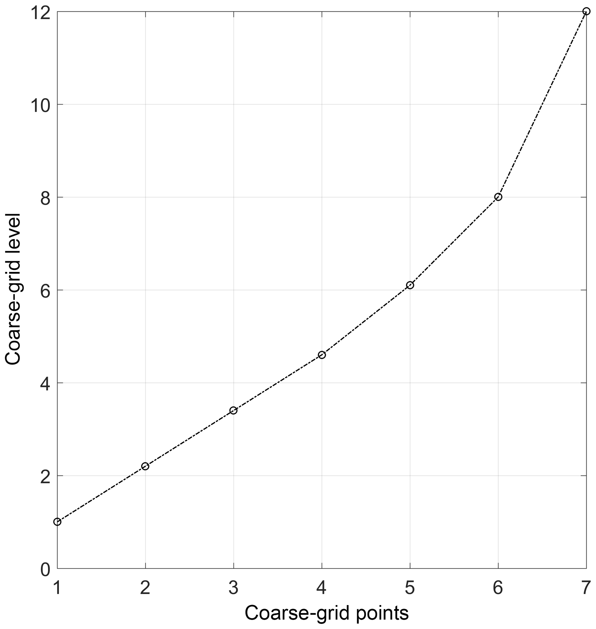
Figure 2The coarse-grid levels are shown for the example case as a function of the cumulative trace of the averaging kernel matrix. The total degrees of freedom for the retrieval is 8.2, which is spread over the entire retrieval grid such that each point has roughly one degree of freedom. As the SNR of the measurements decreases, more fine-grid points are used in the coarse grid, and the distance between points generally increases with altitude.
The resulting coarse grid is then used as the retrieval grid for a second retrieval run. In this paper we will refer to a “run” as one retrieval which typically requires 10 iterations to converge to a solution. However, before running the retrieval again we remove the regularization term in Eq. (4) by choosing an arbitrarily large a priori uncertainty such that the inverse of the a priori covariance matrix () becomes zero. If is set to zero, the optimal estimation becomes the unconstrained weighted least squares solution (vCG), which is the solution of the maximum likelihood problem with the assumption of Gaussian residuals in force. The second retrieval is then a ML retrieval which uses the new coarse retrieval grid calculated from the original first OEM retrieval, and the effect of the a priori is minimal due to minimizing the regularization term. The ML coarse-grid averaging kernels then are unity at all levels.
We now apply our information-centered approach, using the triangular representation from vCG, to lidar OEM retrievals in order to minimize the effect of the a priori information. We will examine the method's effectiveness with RALMO daytime and nighttime water vapor retrievals, as well as with a PCL Rayleigh temperature retrieval. This method is also applicable in general and can be applied to other lidar retrievals. First, we will discuss the results from the triangular representation and the creation of the coarse grid and how it is used as the new retrieval grid. Then we will discuss its effect on the retrieval, vertical resolution, uncertainty budgets, and averaging kernel for a case study for each type of retrieval. We will then discuss the results of the method using representative data sets for all water vapor and temperature retrievals.
5.1 Daytime RALMO water vapor a priori removal
5.1.1 Daytime case study
The daytime water vapor case study retrieval is a 30 min integration obtained in conjunction with a Vaisala RS92 radiosonde launch from the Payerne station on 22 January 2013 at 12:00 UT. This date was chosen because it shows the large impact our method has on low signal-to-noise ratios, which occur during the daytime due to the high solar background or in dry layers (regions with relative humidities less than 25 %). The input data grid for this case was binned to 50 m to remove numerical features in the retrieval due to the high background noise levels.
The diagonal values of the daytime case fine-grid averaging kernels (Fig. 3a) quickly drop below 1 above 2 km due to a dry layer. The measurement response is shown by the red line which first drops below 0.9 at 2.7 km. This is the uppermost altitude at which we consider the retrieval to not have significant influence from the a priori information. The coarse-grid averaging kernels (Fig. 3b), by definition, are all equal to 1 as discussed in Sect. 4 and reach up to 10 km. While the coarse grid ensures that each altitude has 1 degree of freedom, we do not necessarily consider the entire retrieval as meaningful, which will be discussed further below. The vertical resolution of each point on the fine and coarse retrieval grids is shown in Fig. 4. In this case, the fine-grid averaging kernels are never exactly 1, and therefore have some a priori information, which explains why the resolution of the fine-grid retrieval is still a little bit coarser than the grid width. The vertical resolution of the coarse-grid retrieval is still a bit worse. This is attributed to the loss of a fractional degree of freedom, resulting from Eq. (12). The penultimate point in the coarse retrieval grid has a vertical resolution of over 600 m. The coarse-grid points which have incorporated more fine-grid points have a lower vertical resolution than others (i.e., the points between 2.8 and 10 km altitude).
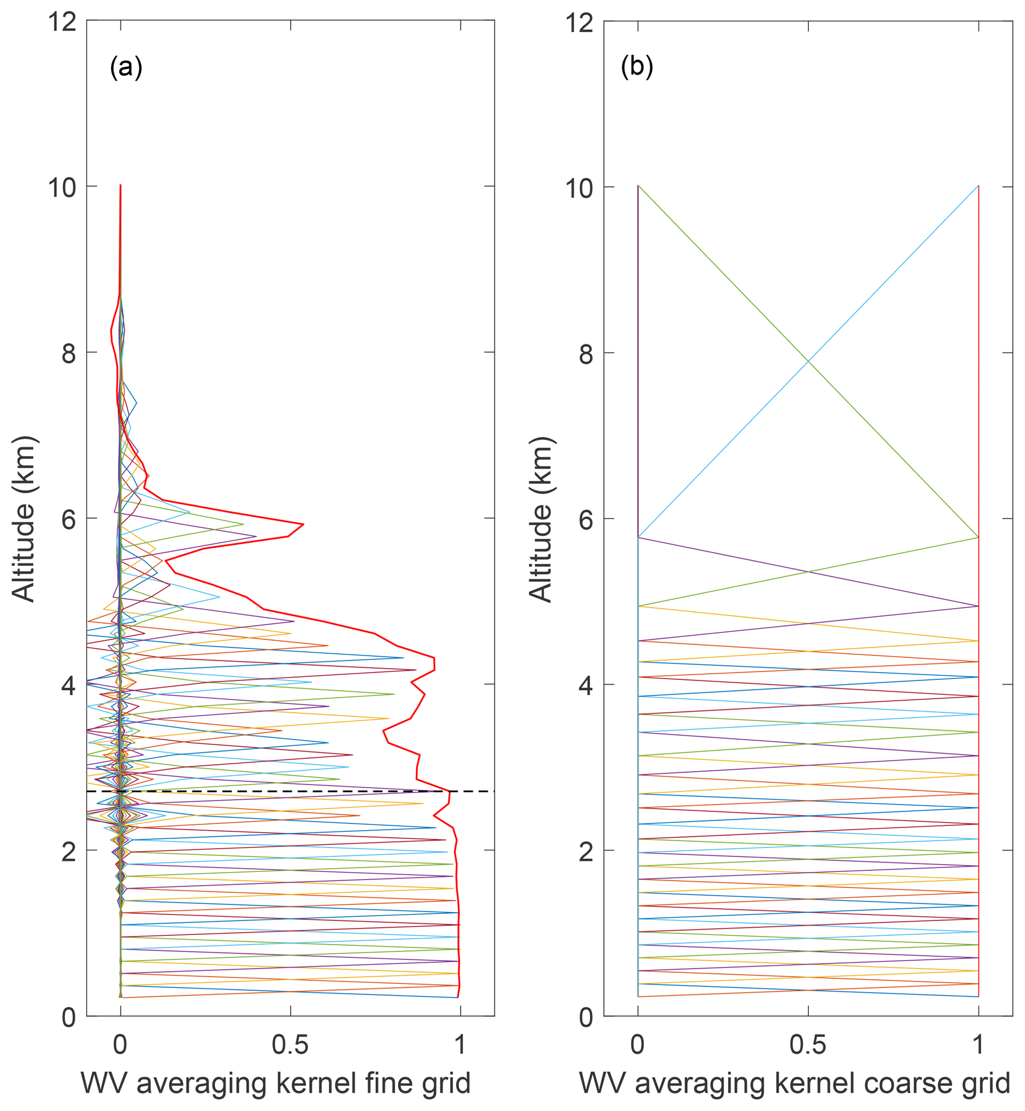
Figure 3The clear-sky daytime water vapor averaging kernel matrix for 22 January 2013 at 12:00 UT (a) on the fine grid and (b) on the coarse grid. Every other averaging kernel has been plotted for clarity. (a) The measurement response Au is the red solid line. The horizontal dashed line is the height at which the measurement response is first equal to 0.9 and is the line above which we would consider there to be large influence from the a priori. (b) The coarse-grid averaging kernels all equal 1 and reach up to the last retrieval altitude at 10 km.
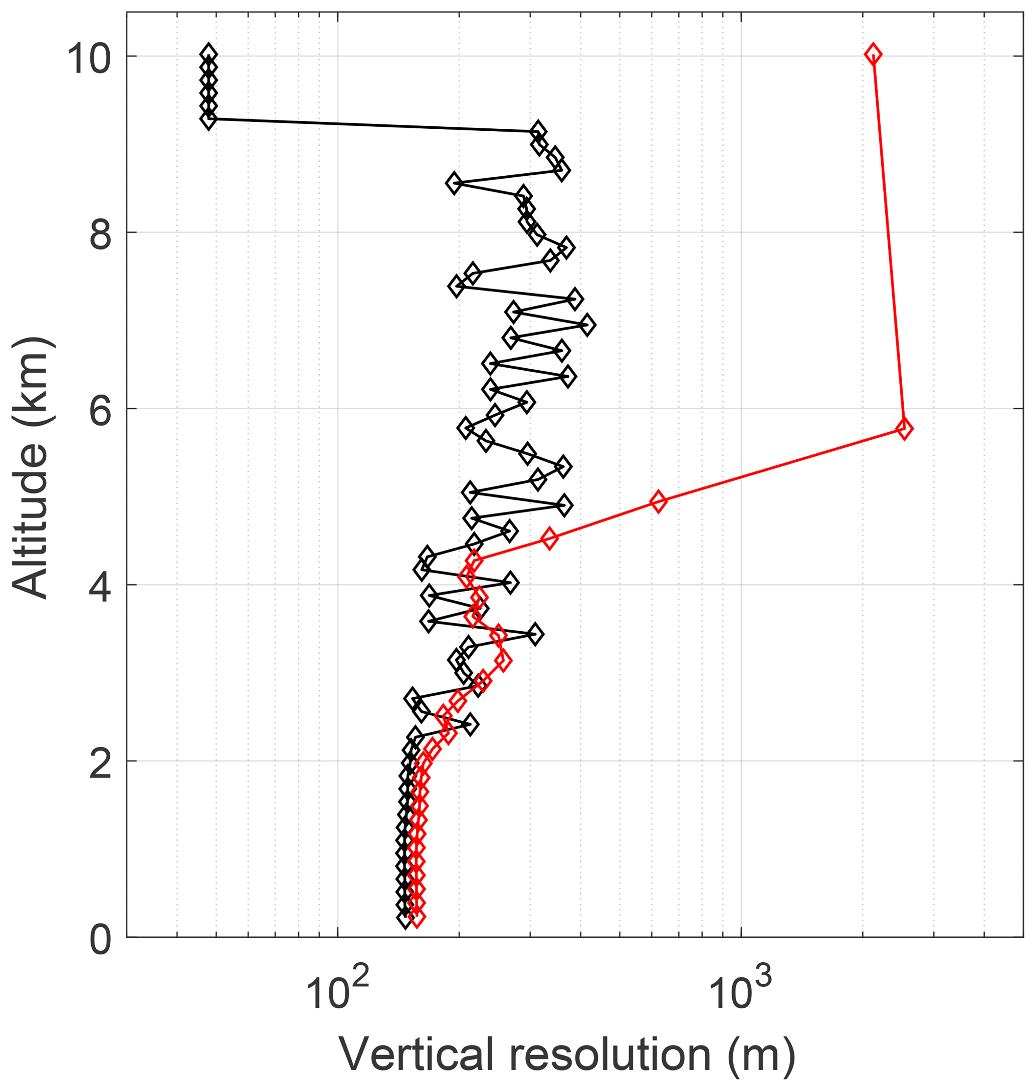
Figure 4The vertical resolution profile on 22 January 2013 12:00 UT. The vertical resolution will decrease on the coarse grid as the points are used to reach one degree of freedom. The last two points have vertical resolutions of several hundred meters but are not considered meaningful points as they have total uncertainties larger than 60 %.
The daytime water vapor fine- and coarse-grid retrievals are shown in Figs. 5a and b respectively. The fine- and coarse-grid retrievals are the same up to 2.5 km, at which point the coarse-grid retrieval (in red) begins to more closely follow the path of the radiosonde and the traditional profile (dotted blue) and not the fine-grid retrieval (black). The coarse-grid retrieval agrees with the radiosonde until 4.5 km. At 4.8 km the statistical uncertainty is above 100 %, and the last two points are above 80 % statistical uncertainty; therefore, the retrieval is no longer meaningful at these altitudes. All valid points are below the red dotted line. The large peaks in the fine-grid retrieval above 5 km show features that are not physical. If we consider the last valid point to be 4.5 km with a statistical uncertainty of 27 %, the a priori removal method extends the valid altitude range of the daytime OEM retrievals by 2 km.
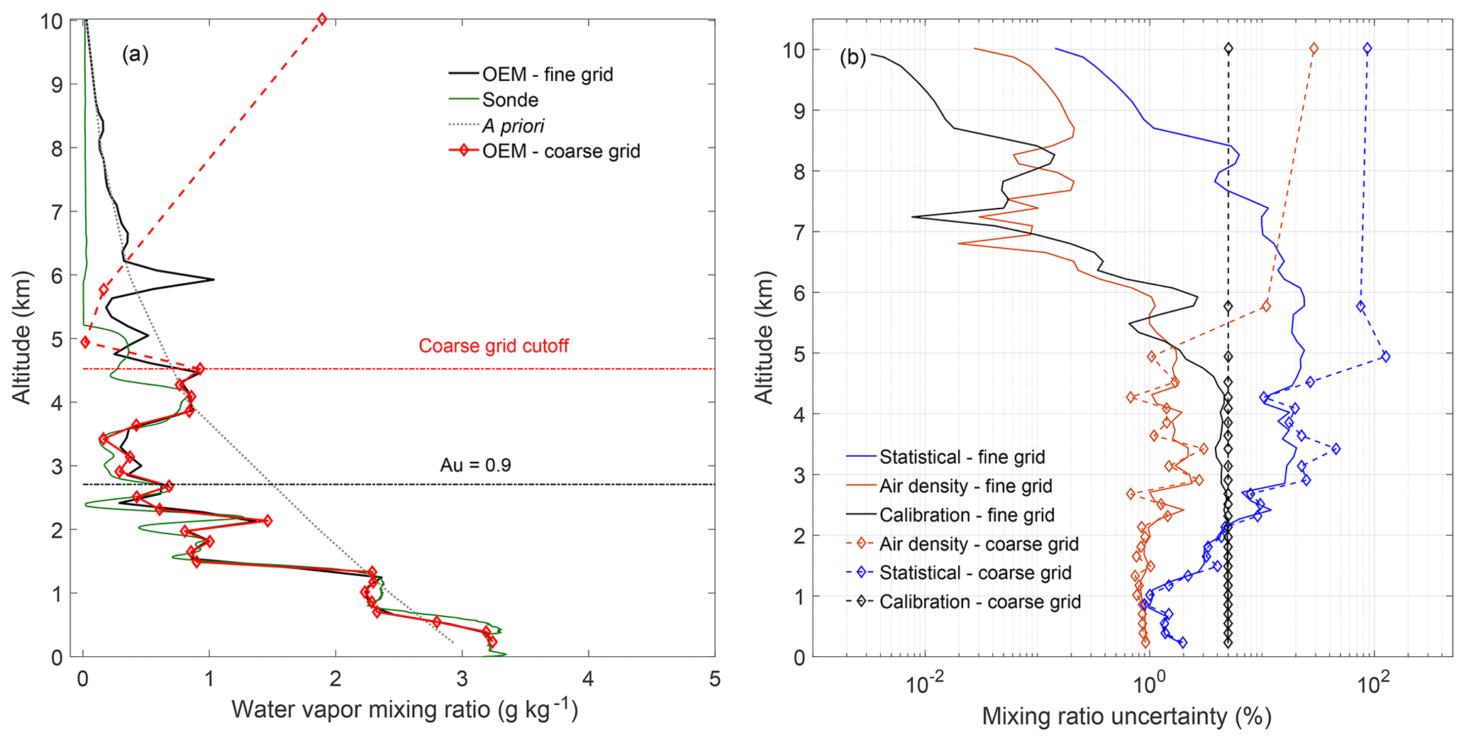
Figure 5(a) The retrieved daytime water vapor profile for 22 January 2013 12:00 UT. The fine-grid retrieval is in black and includes the a priori information. The coarse-grid retrieval is in red and the a priori (grey) has been removed. The radiosonde is shown in green. The points which we do not consider meaningful because their uncertainties are larger than 80 % in the retrieval are shown in dashed red lines. The coarse-grid retrieval increases the last valid point by 2 km (red dashed line) and now more closely resembles the radiosonde above the original cutoff altitude of 2.7 km (black dashed line). (b) The three primary contributors to the uncertainty budget on 22 January 2013 12:00 UT are shown for comparison: the statistical uncertainty, the uncertainty due to the calibration constant, and the uncertainty due to air density. The solid lines are the relative uncertainties from the fine-grid retrieval, and the dashed lines are from the coarse-grid retrieval. The a priori begins influencing the profile above 2 km where the uncertainty increases.
The three main components of the uncertainty budget are shown in Fig. 5b. The uncertainties shown in this study are relative percent uncertainties, e.g., the uncertainty value divided by the quantity times 100. The fine-grid statistical and air density uncertainties increase with altitude due to decreasing SNR of the return photo counts and then decrease as the retrieval falls back to the a priori value as the signal goes to zero. The coarse-grid statistical uncertainties and the uncertainty due to air density continue to increase with altitude, instead of falling back to zero, on the coarse grid because the a priori information has been removed. The a priori information has been removed by setting the inverse covariance matrix to zero in Eq. (5). When the a priori covariance is removed, the solution space is no longer constrained and the coarse-grid uncertainties increase compared to the fine-grid uncertainties. The calibration uncertainty also increases but now remains constant at all altitudes with the exception of the last point, as it is no longer influenced by the a priori constraint.
Since the measurement response of the unconstrained coarse-grid retrieval is unity everywhere by definition, this quantity is not an adequate criterion for determining the last useful altitude of a retrieval. Therefore, we use the uncertainty of the retrieval as a criterion instead. A relative uncertainty of 60 % was chosen as the largest acceptable error, which resulted in a cutoff height of 4.5 km altitude. We found this height to correspond with the altitude at which the signal-to-noise ratio decreases below 1 and noise begins to dominate the retrieval. However, the choice of the critical uncertainty is a matter of preference, and depending on the goal of the research it may be more preferable to cut the retrieval at a lower uncertainty. It is also important to take the presence of dry layers into account to avoid cutting the profile too low if the uncertainty threshold is lowered. It may also be more useful to determine a threshold based on absolute errors instead of relative, particularly for the case of dry regions with low signal. To maintain consistency with Sica and Haefele (2015, 2016), we have chosen to use relative errors for this analysis. The second-to-last point in the statistical uncertainty has a mixing ratio uncertainty of 100 % due to the lack of signal above 4.5 km. Therefore, the ML coarse-grid retrieval was cut to include measurements below 4.5 km. The maximum uncertainty is 46 % statistical uncertainty at 3.8 km, where the water vapor signal is very small due to the presence of a dry layer at that altitude. A dry layer is a layer where the water content has below 25 % relative humidity. The relative humidity measured by the radiosonde at 3.8 km is 10 %. While the a priori removal technique increases the maximum retrieval altitude, in addition to removing the contribution from the a priori profile, it will increase the statistical uncertainty of the retrieval as well. It should, however, be noted that uncertainties of OEM and maximum likelihood retrievals signify different things. The OEM uncertainties characterize the a posteriori knowledge including a priori and measurement information, while the maximum likelihood uncertainties characterize the pure measurement information.
Finally, we compare the fine- and coarse-grid retrievals with the radiosonde profile in Fig. 6. To highlight the differences in the OEM fine- and ML coarse-grid retrievals, we have interpolated the radiosonde onto both the fine and coarse grids for comparison, and the 1σ uncertainties in the percent difference are shown as the shaded regions on each side of the percent difference profile. The radiosonde uncertainties used to calculate the percent difference uncertainties were calculated by propagating pressure, temperature, and relative humidity uncertainties through the mixing ratio formulae of Hyland and Wexler (1983). The uncertainty values were assumed constant with height using the values presented in Dirksen et al. (2014). The percent difference calculated on the fine grid is cut at the 0.9 measurement response cutoff height. At all altitudes the retrievals agree with the radiosonde within their respective 1σ uncertainties. The large uncertainties and the large difference from the radiosonde at 2.2 km are due to the presence of a dry layer where the signal is much weaker. The radiosonde detects much less water vapor compared to both lidar retrievals. That altitude is not included in the coarse-grid retrieval due to its lack of information; therefore a similar feature is not seen in the coarse-grid percent difference profile.
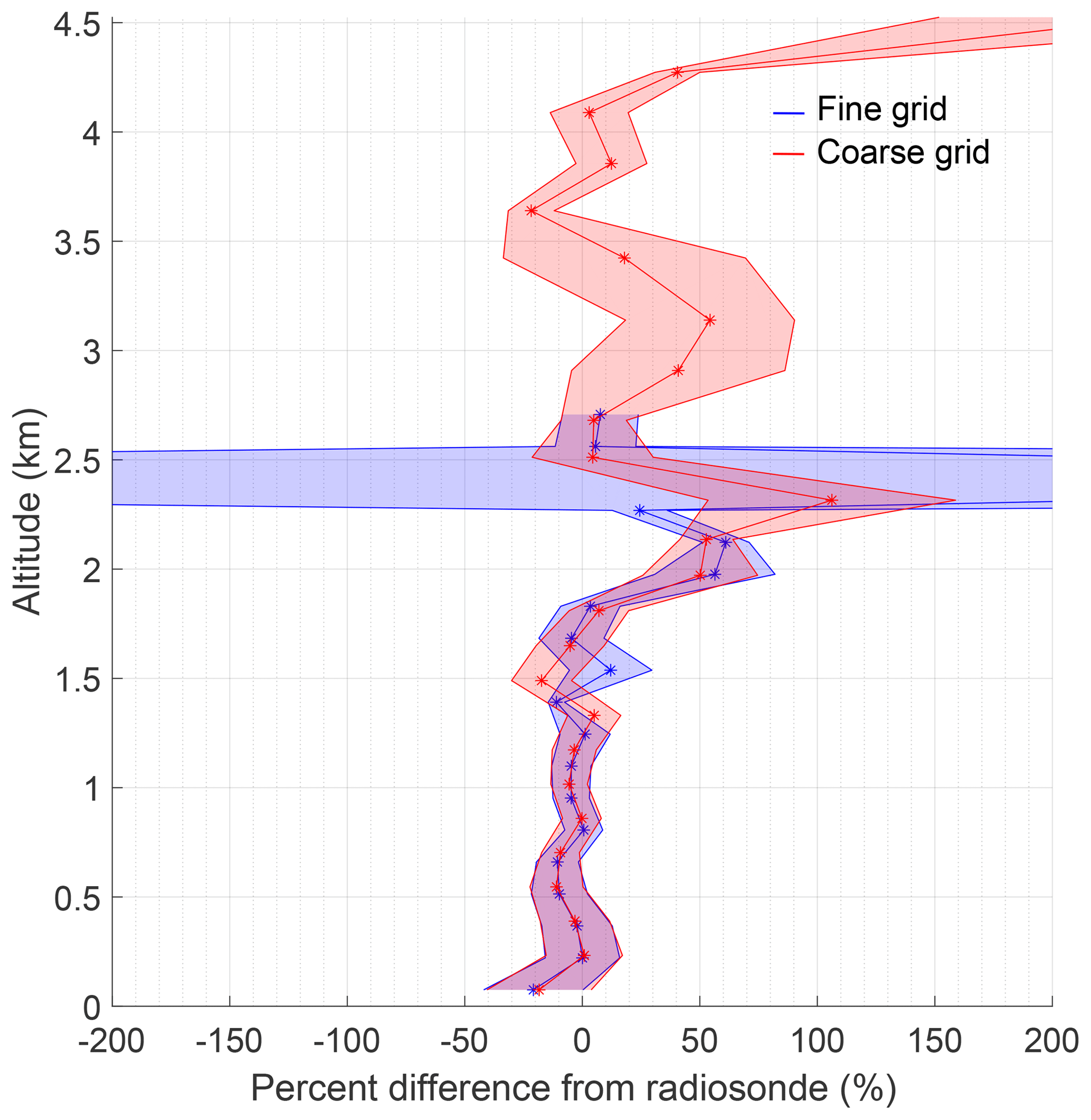
Figure 6The relative percent difference between the radiosonde and the fine- and coarse-grid retrievals on 22 January 2013 12:00 UT. The 1σ uncertainties for percent difference are shown as shaded regions. The fine-grid results are shown in blue and the coarse-grid results in red. The largest percent difference for the fine grid is 600 % and is not shown.
5.1.2 Daytime representative data set
The a priori removal technique was tested on 5 additional days to study the differences between the fine- and coarse-grid cutoff heights as well as their agreement to the radiosonde (Fig. 7). The daytime water vapor OEM profiles typically reach up to around 3–5 km on the fine grid and up to 6 km on the coarse grid. There is an average of 1.5 km difference between the two cutoff heights. In some cases, the differences are much larger, and this is usually due to the presence of dry layers causing the averaging kernel to decrease at a lower altitude. The large difference between the final altitudes on each grid is typically due to a slow decrease in averaging kernel values with height, as was shown in the case study. Additionally, in some cases, such as on 28 February 2012, the uncertainty never rose above 60 %, in which case the second-to-last point on the coarse grid was chosen as the cutoff point.
The daytime water vapor OEM fine- and coarse-grid profiles show similar differences to the radiosonde profile within their respective uncertainties. For each case, with the exception of 5 May 2009, there are very few differences between the fine- and coarse-grid retrievals from the radiosonde. On 5 May 2009, the coarse-grid retrieval was shifted with respect to the fine-grid OEM retrieval, possibly due to poor calibration on that day.
The daytime fine- and coarse-grid retrievals agree with radiosonde measurements within their respective uncertainties, and the coarse-grid retrievals significantly increase the final meaningful retrieval altitude by an average of 1.5 km. Daytime water vapor retrievals are often limited in altitude due to the high solar background in both the water vapor and nitrogen channels. Increasing the final meaningful altitude by up to 2 km is highly valuable for forecasting and validation purposes.
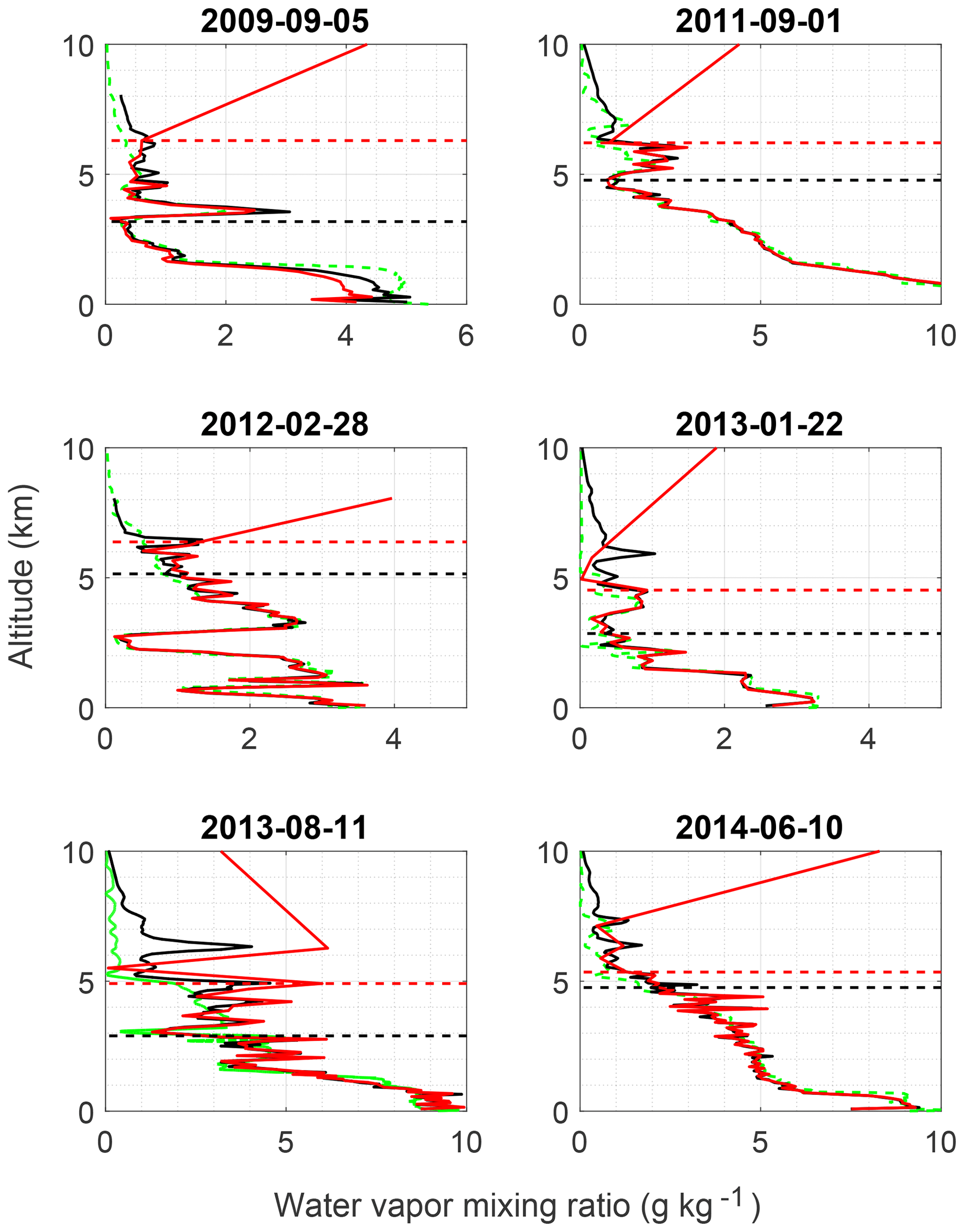
Figure 7Daytime water vapor mixing ratio retrievals for 5 additional nights. Black lines are the original OEM retrieval on the fine grid, red solid lines are the ML coarse-grid retrievals, and the dashed green lines are the radiosonde mixing ratio measurements. The black dashed line is the original 0.9 measurement response cutoff height, and the red dashed lines are the coarse-grid cutoff heights which were chosen as the last altitude whose measurements had less than 60 % total uncertainty.
5.1.3 Examining cutoff heights using signal-to-noise ratios
To confirm our choice of cutoff heights for the fine- and coarse-grid retrievals, we looked at the SNR profiles for the digital water vapor signal for each of the daytime comparisons (Fig. 8). The water vapor signals are roughly 10 times weaker than the nitrogen signal and therefore determine the amount of information available to the retrieval. The SNR profiles were calculated using the raw digital input signals to the OEM retrieval. As digital signals follow Poisson statistics, the SNR was calculated using the following equation:
where z is altitude, N is the number of photon counts, and B is the mean background signal calculated as an average of the counts from 55 to 60 km for the water vapor measurements.
It stands to reason that as the SNRs of the measurements drop, the OEM dependence on the measurements should also decrease (and the a priori's increase) due to the increase in noise. Typically, the SNR level drops below between 3 and 4 km altitude for daytime measurements due to the high solar background. The 0.9 measurement response cutoff height used for the fine-grid OEM results is shown by the blue dashed line in Fig. 8. For each daytime retrieval, the 0.9 measurement response cutoff falls between a SNR of 1 and 2. The green dashed lines are the last heights at which the measurement response is larger than 0.8. The 0.8 cutoff is consistently located at the heights were the signal-to-noise ratio is unity and usually 500 m to 1 km or higher than the 0.9 cutoff. The coarse-grid cutoff height, shown by the red dashed line, corresponds typically to the boundary where the SNR drops below 1 into the region where noise dominates. The location of the coarse-grid cutoff then makes sense, as this would be the altitude where no more information could be gathered and the uncertainties increase beyond what we would consider meaningful or useful. The coarse-grid cutoff sometimes coincides with the location of the 0.8 cutoff but is typically below the coarse-grid point. The SNRs of the 0.9 measurement response cutoff correspond to the traditional limits of water vapor measurements for the RALMO lidar, which are typically cut where the water vapor SNR drops below 2. Therefore, for a fine-grid OEM retrieval, we find that the 0.9 cutoff is a consistent choice with regards to the traditional method. The 0.8 cutoff height could be used, but we would caution against it as it may induce unwanted amounts of a priori water vapor information into the retrieval. The coarse grid utilizes the amount of information available from the measurements to produce an information-centered profile; therefore, we also find its height appropriate as it borders where the noise begins to dominate the measurements.
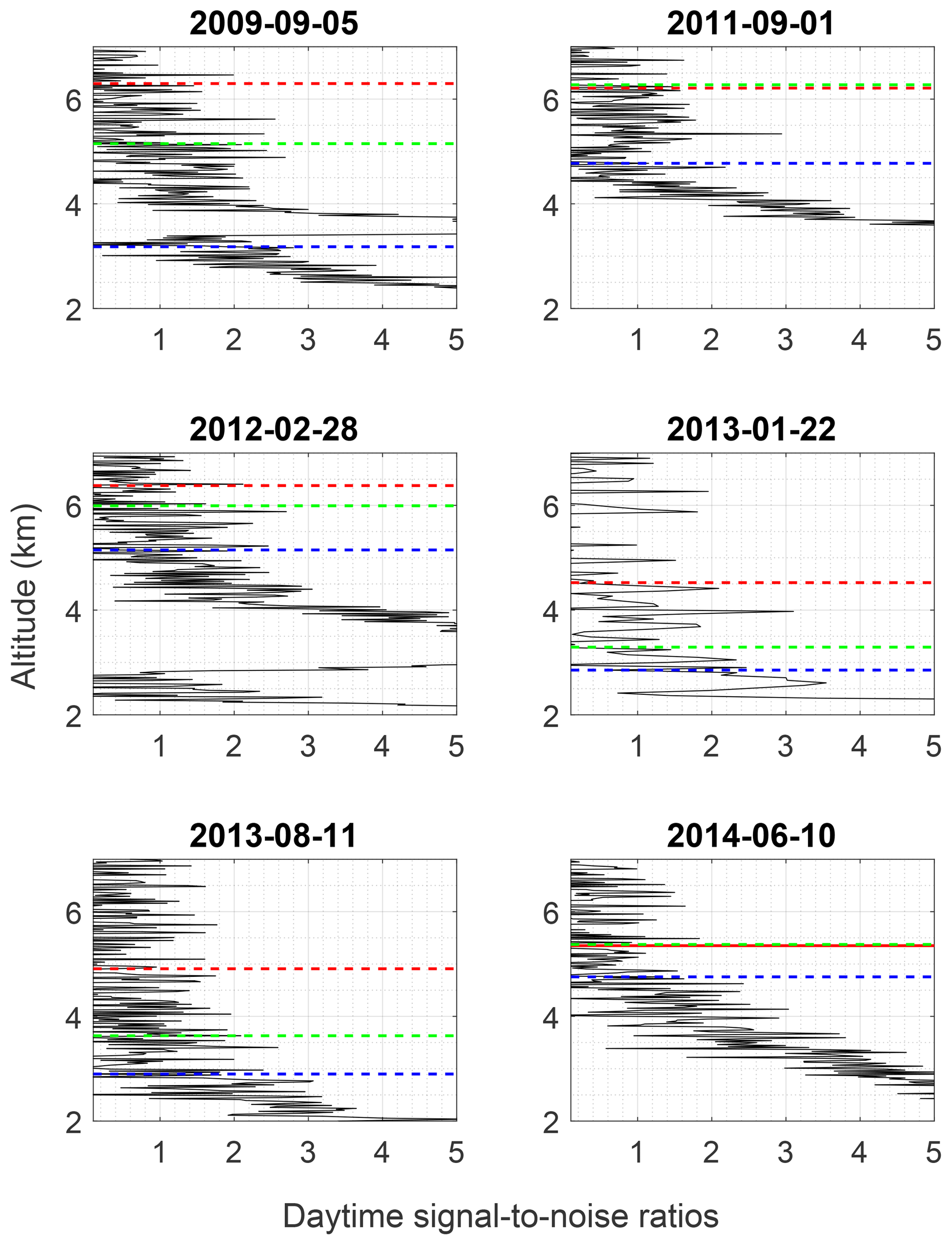
Figure 8Daytime water vapor SNRs (black). The various cutoff heights are shown in dashed lines. The 0.9 measurement response cutoff is blue, the 0.8 measurement response cutoff is green, and the coarse-grid cutoff is in red.
5.2 Nighttime RALMO water vapor a priori removal
5.2.1 Nighttime case study
The nighttime case study retrieval uses a 30 min integration on 24 April 2013 00:00 UT which coincides with the time of radiosonde launch. The fine retrieval grid for the RALMO water vapor retrieval is 50 m.
The averaging kernel matrix for the fine- and coarse-grid retrievals is shown in Fig. 9a and b, respectively. The altitude where Au first equals 0.9 for the fine-grid retrieval is at 9.1 km, which is typical for a 30 min nighttime measurement. The coarse-grid averaging kernels all equal 1, with the second-to-last altitude at 11 km.
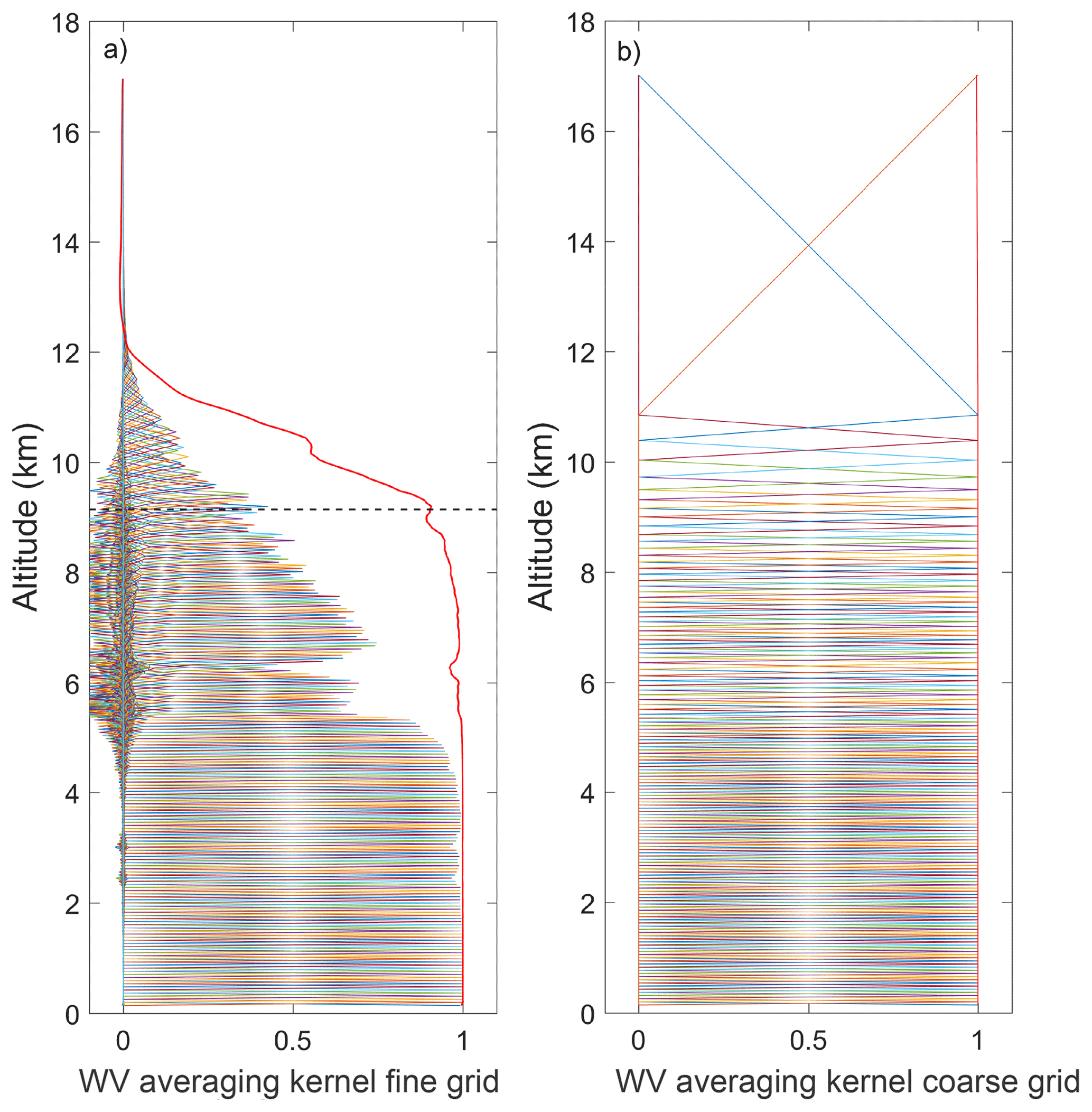
Figure 9The averaging kernel matrix for the nighttime water vapor retrieval on 24 April 2013 00:00 UT. (a) The fine-grid retrieval with a maximum altitude of 9.1 km (black dashed line). The measurement response is shown in red. (b) The coarse-grid retrieval, where each averaging kernel is 1 for all altitudes.
Unlike the daytime case, the nighttime vertical resolution between the fine- and coarse-grid retrievals is very close up to 5 km where they begin to diverge (Fig. 10). This is because the nighttime averaging kernels are very close to 1 until 5 km. As the a priori information enters the signal, more points from the fine grid are used to create the coarse grid, resulting in larger coarse-grid averaging kernels and decreasing the vertical resolution.
Figure 11 shows the final water vapor retrievals on the fine and coarse grid as well as a Global Climate Observing System (GCOS) Reference Upper-Air Network (GRUAN) Vaisala RS92 radiosonde profile. Both fine- and coarse-grid profiles agree past the 0.9 cutoff and up to 9 km, at which point the coarse-grid retrieval diverges from both the fine-grid retrieval and the radiosonde. We do see small differences in dry layers where the signal level is lower; however, the differences are inside the total uncertainty. The last four points in the retrieval are shown in dashed lines because we do not consider them to be meaningful points as their total uncertainties are 70 % or larger.
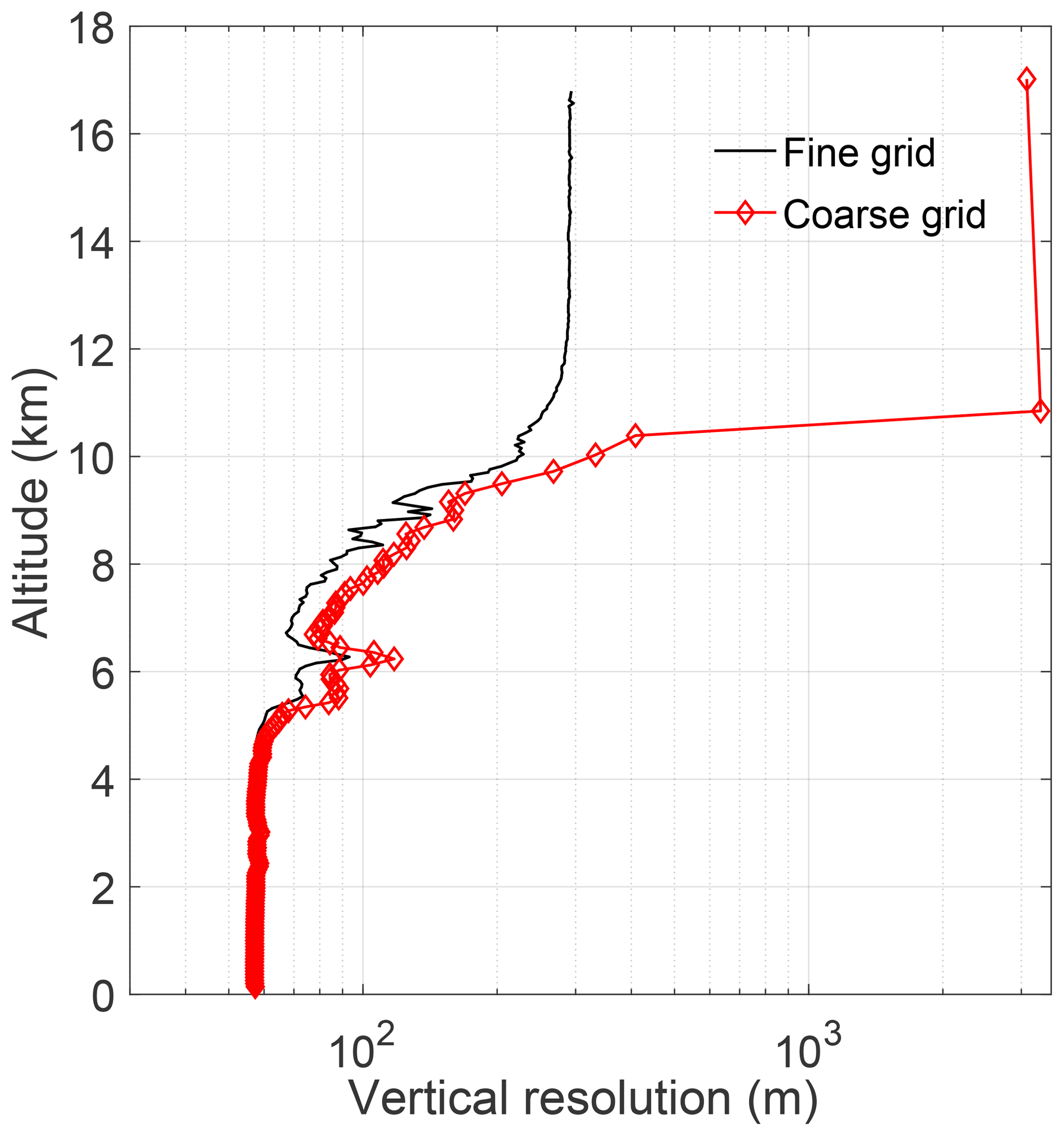
Figure 10The vertical resolution for 24 April 2013 00:00 UT. The vertical resolution on the coarse-grid retrieval decreases as more points are added to ensure that each bin has one degree of freedom. The coarse-grid resolution is shown in red and each point is marked. The fine grid has points every 50 m; therefore they are not shown individually.
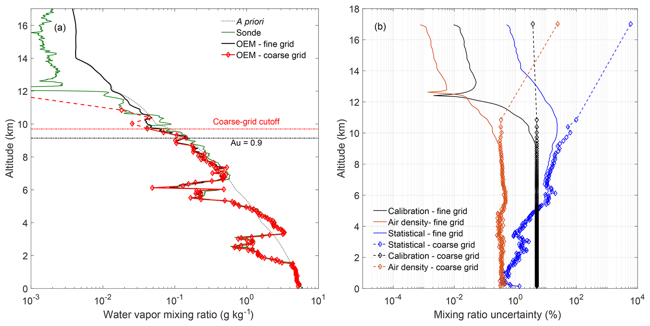
Figure 11(a) The water vapor retrieval for 24 April 2013 00:00 UT. The fine-grid retrieval is in black; the coarse-grid retrieval is in red. In general, both OEM retrievals on the coarse and fine grid and the radiosonde agree until the original cutoff altitude at 9.1 km (dashed black line). The dashed red lines above 9.7 km show the points we do not consider meaningful due to their large uncertainties. Therefore, the a priori removal technique increases the last altitude bin by 600 m. The method is limited by the lack of water vapor in the upper troposphere which causes a large and rapid drop in signal. (b) The three largest relative uncertainty components are compared here on the fine and coarse grid. The drawback of the a priori removal technique is that while you gain in altitude, you increase the uncertainty. At 9.7 km the statistical uncertainty is 52 %, above which is where we no longer consider the rest of the retrieval to be viable.
The uncertainties for the nighttime retrievals are shown in Fig. 11b. Similarly to the daytime retrievals, we have shown the top three uncertainty contributors for comparison. Below 5 km the uncertainties are the same, as there is no influence from the a priori information. However, above 5 km the uncertainties begin to increase due to the removal. The statistical uncertainty increases to almost 100 % uncertainty at the second-to-last point due to the lack of signal above 11 km. The mixing ratio uncertainty due to the calibration uncertainty is now constant with altitude, which we would intuitively expect, and contributes roughly 5 % uncertainty to the mixing ratio measurements. The uncertainty due to air density increases by a maximum of 0.2 % at the second-to-last point. We would consider anything above 9.7 km to be invalid since points above that height have a total uncertainty of 60 % or higher. The last valid point has a total uncertainty of 52 % at 9.7 km. Therefore, the a priori removal technique increases the maximum valid altitude of the retrieval by 600 m.
The fine- and coarse-grid retrievals do not change very much with respect to each other until 9.1 km where the averaging kernels begin to drop off significantly. They both produce similar differences with the radiosonde (Fig. 12), except between 5 and 7 km, likely due to the dry layer present at those altitudes and smoothing from the coarser grid. The uncertainties for the nighttime percent differences are more variable than the daytime percent difference uncertainties due to the fact that we used a GRUAN RS92 radiosonde on this night which calculates the uncertainties of the radiosonde as a function of altitude. Mixing ratio uncertainties were calculated in the same way as the daytime radiosonde mixing ratio uncertainties.
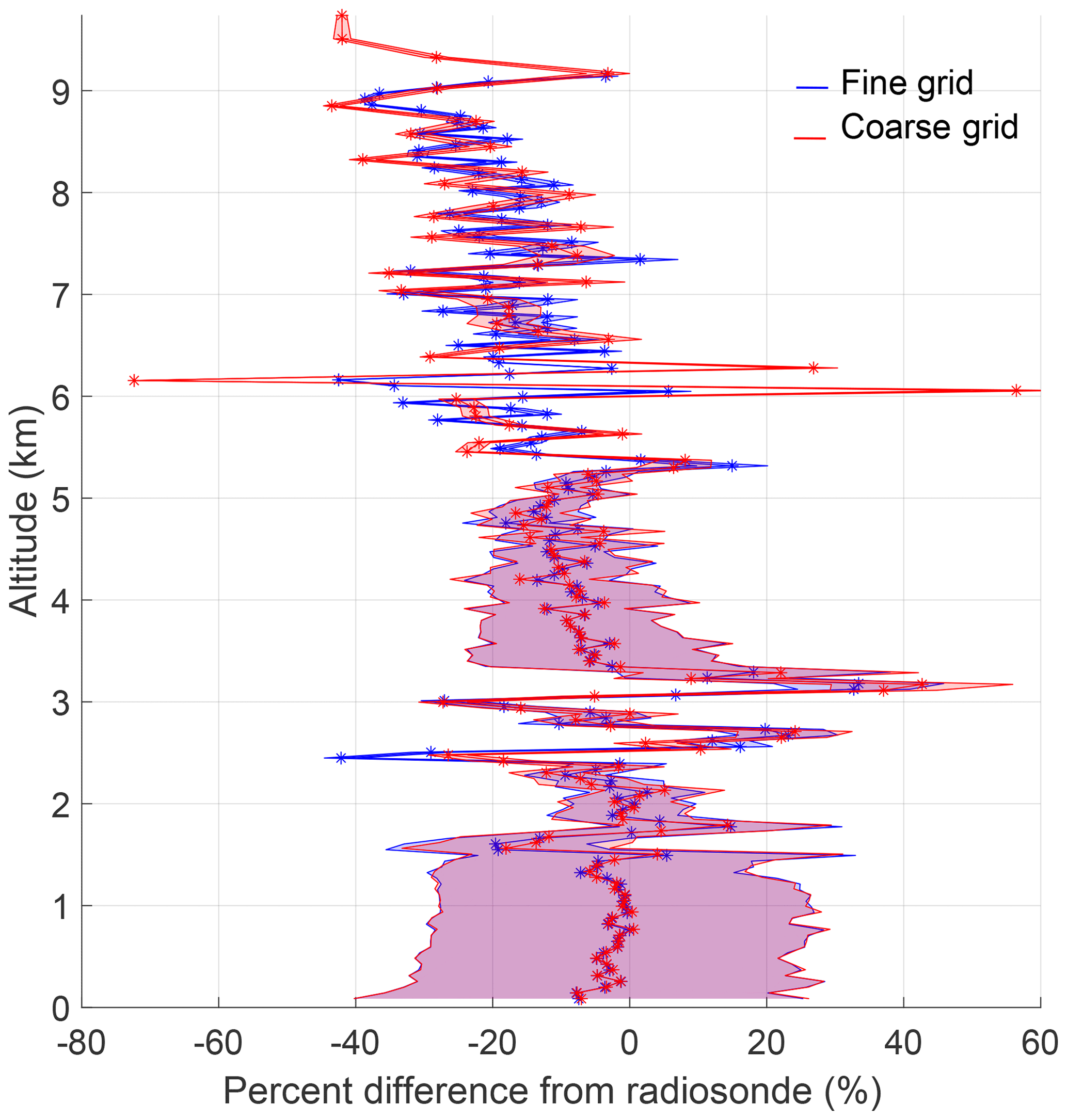
Figure 12The percent difference from the radiosonde for both the fine- and coarse-grid retrievals. Both show similar differences with the radiosonde and the last valid height is 9.7 km.
5.2.2 Nighttime representative data set
The a priori removal method was applied to eight additional nighttime retrievals (Fig. 13). The nighttime cutoff heights in Fig. 13 show a general increase in cutoff height when using the a priori removal method, albeit not as large. As with the daytime retrievals, the coarse-grid cutoffs were chosen to be the last altitude below with a total uncertainty less than 60 %. Choosing a maximum uncertainty of 40 % would result in cutoff heights closer to the original fine grid's. In all cases, the coarse grid increases the maximum acceptable altitude, however, in some cases by only a few hundred meters. On those nights, the averaging kernels decrease quickly after the original fine-grid cutoff height; therefore there is very little information with which to create the coarse grid.
In all cases, the water vapor nighttime OEM fine-grid and ML coarse-grid retrievals produced profiles which agreed with the radiosondes within their respective uncertainties. Differences larger than 0.4 g kg−1, between both retrievals and the radiosonde profile, can be seen on 25 May 2012. This was likely due to lack of colocation with the lidar, as the balloon was 10 km away from the lidar at that altitude.
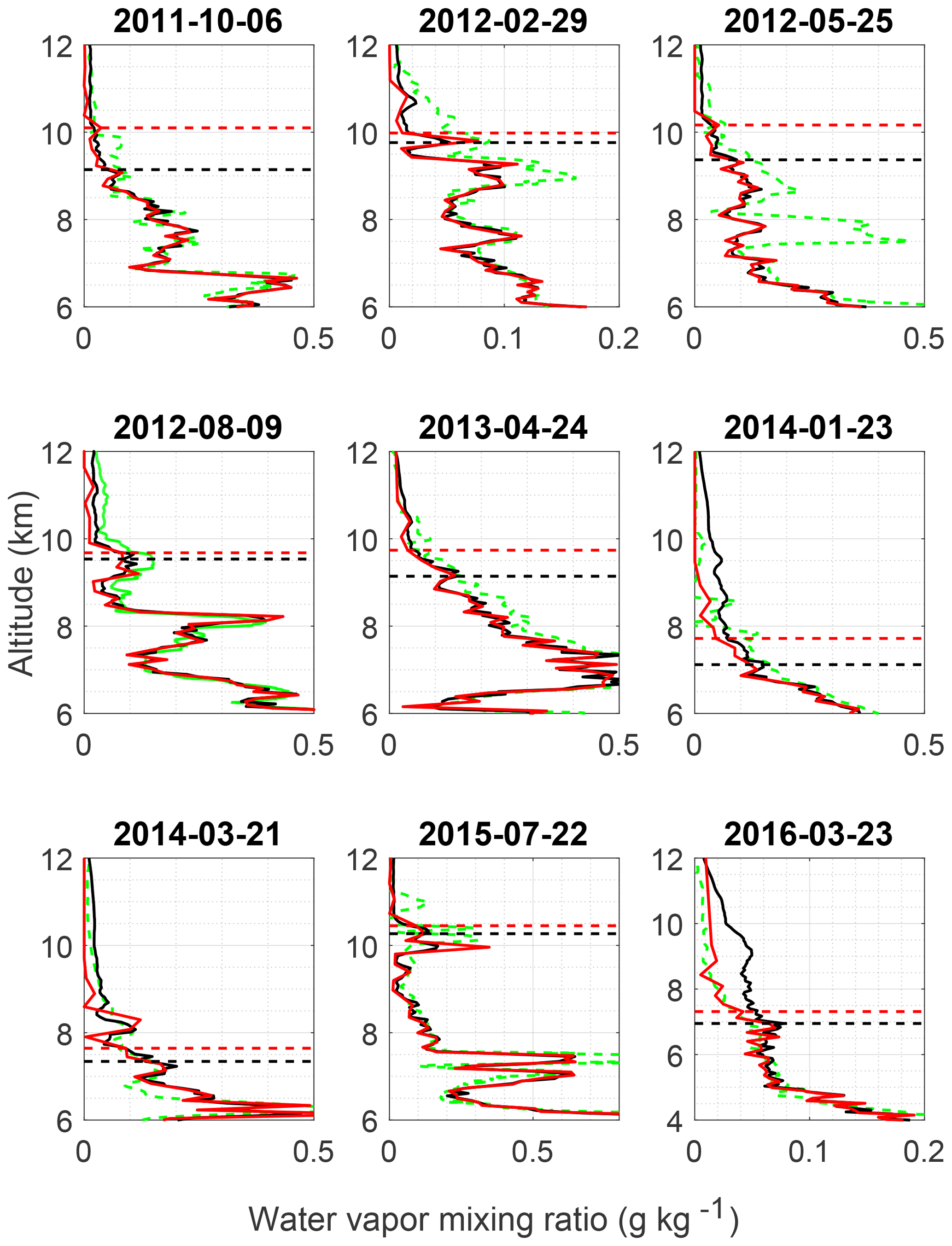
Figure 13All nighttime water vapor retrievals. The radiosonde is shown by the green dashes, the fine-grid retrieval in black, and the coarse-grid retrieval in red. The 0.9 cutoff height for the fine grid is shown by the black dashed line, while the coarse-grid cutoff height is the horizontal red dashed line.
Using the a priori removal technique for nighttime retrievals may be helpful when trying to improve water vapor measurements of the upper troposphere and lower stratosphere (UTLS) region. However, in this case, because the nighttime measurements have large SNRs and a rapid change from high to low signal values, we do not see as large of a difference between the coarse- and fine-grid retrievals as we do in the daytime retrievals. For nighttime retrievals, the coarse grid may not provide an operational advantage but can still be used to homogenize a data set for trend analysis or climatological studies which would require no a priori influence. This will be discussed further in Sect. 6.
5.2.3 Nighttime cutoff heights and SNRs
Similarly to the daytime water vapor measurements, we have also compared the SNR values with the fine-grid and coarse-grid cutoff heights (Fig. 14). As before, the fine-grid 0.9 measurement response cutoff corresponds to the last point where the measurement response is greater than 0.9 and is shown by the blue dashed line in Fig. 2. We have also included the 0.8 measurement response cutoff height (green dashed line) for comparison, which is calculated in the same way as the 0.9 measurement response cutoff. Lastly, we have included the cutoff height for the coarse grid, chosen as the last height at which the total uncertainty of the retrieval is less than 60 %.
In all cases, the 0.9 measurement response cutoff corresponds to a SNR of 2. When we compare the 0.8 measurement response cutoff height with the 0.9 cutoff height, we see that the 0.8 cutoff is typically between a few hundred meters to 1 km higher. However, unlike the daytime measurements, the 0.8 cutoff and the coarse-grid cutoff are very close and are either close to 1 or at the boundary where the SNR starts to be noise-dominated. Therefore, we would suggest when using fine-grid nighttime OEM water vapor retrievals to use the 0.9 measurement response as a cutoff height since the 0.8 cutoff height may be in the region where noise dominates, which would lead to larger amounts of the a priori entering the retrieval.
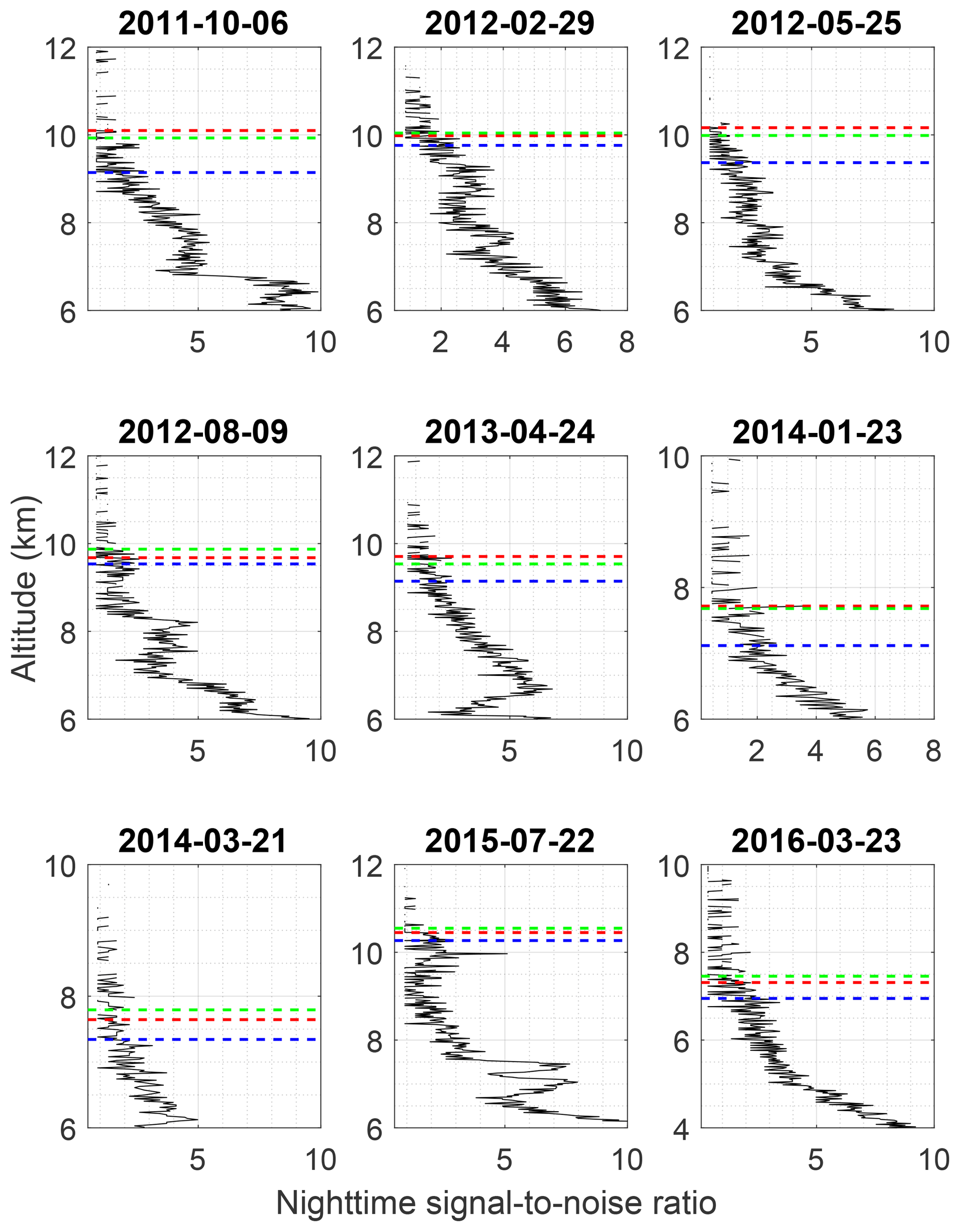
Figure 14Nighttime SNR calculations for each nighttime water vapor OEM retrieval. The dashed lines are the corresponding cutoff heights: 0.9 measurement response (blue), 0.8 measurement response (green), and coarse grid (red).
5.3 Purple Crow Lidar Rayleigh temperature a priori removal
We picked a sample night, 12 May 2012, from the Rayleigh temperature climatology in Jalali et al. (2018) to illustrate the a priori removal procedure for a Rayleigh temperature retrieval. The original OEM retrieval fine grid was 1024 m, and the a priori temperatures were taken from the CIRA-86 model. The details regarding the OEM retrieval are discussed in Sica and Haefele (2015), and its results applied to the climatology are discussed in Jalali et al. (2018).
The averaging kernels for the fine-grid and coarse-grid retrievals are shown in Fig. 15a and b. The red line is the measurement response or the estimate of the averaging kernel's sensitivity to the measurements. The height at which the measurement response equals 0.9 was chosen as a cutoff height in Jalali et al. (2018), which is shown in Fig. 15a with a dashed line. After applying the a priori removal, the averaging kernel on the coarse grid is equal to 1 at each point. Fig. 15b shows that at the coarse-grid points, according to the averaging kernel, the temperature retrieval is completely sensitive to the measurements and therefore there is no a priori contribution.
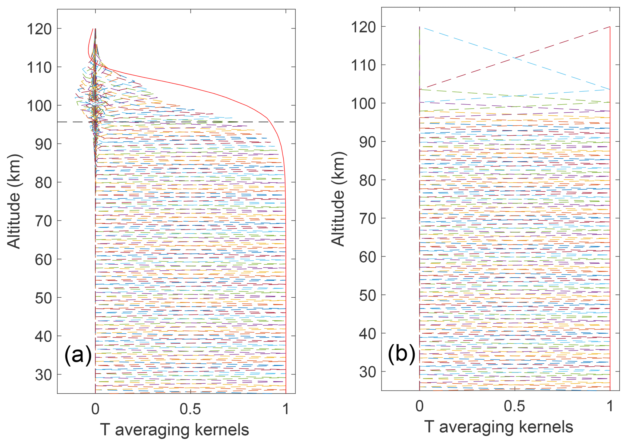
Figure 15The PCL averaging kernels for the temperature retrieval on 12 May 2012 on the fine grid (a) and on the coarse grid (b). The Au=0.9 cutoff height on the fine grid is shown by the black horizontal dashed line at 97 km. The red lines on the edges of the averaging kernels are the measurement response. The coarse grid extends the temperature upwards by 4 km.
The vertical resolution for both grids is similar up to 85 km altitude (Fig. 16). Above this height the coarse grid incorporates more points from the fine grid, and thus the vertical resolution decreases. The values of the vertical resolution (Fig. 16) of the two highest points for the coarse grid are 10 km at 100 km and 8 km at 110 km. However, the corresponding total uncertainties at these altitudes are above 100 % and 60 %; therefore we do not consider them to contribute to the retrieval.
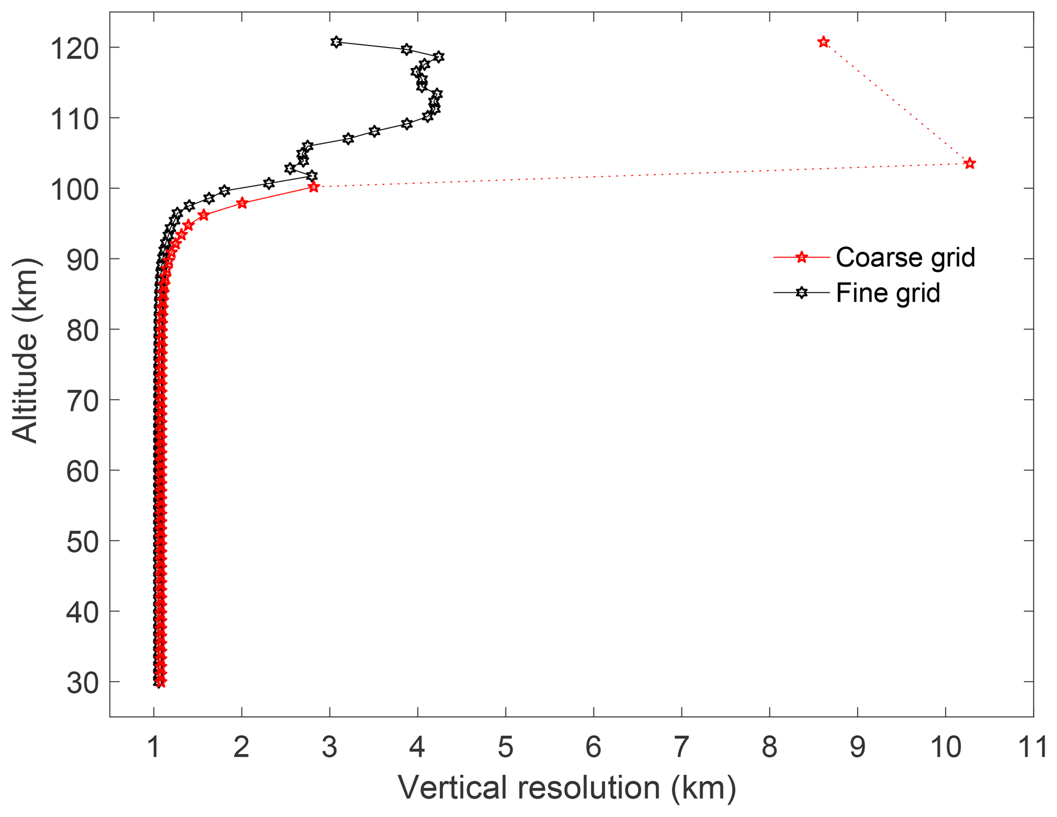
Figure 16The PCL vertical resolution for 12 May 2012 on the fine and coarse grid. The vertical resolution is similar up to 85 km on both grids. Above this height the vertical resolution decreases until it is 10 km in resolution above 100 km altitude (dotted red line). We consider 100 km to be the highest meaningful point on the coarse grid due to large uncertainties above that height.
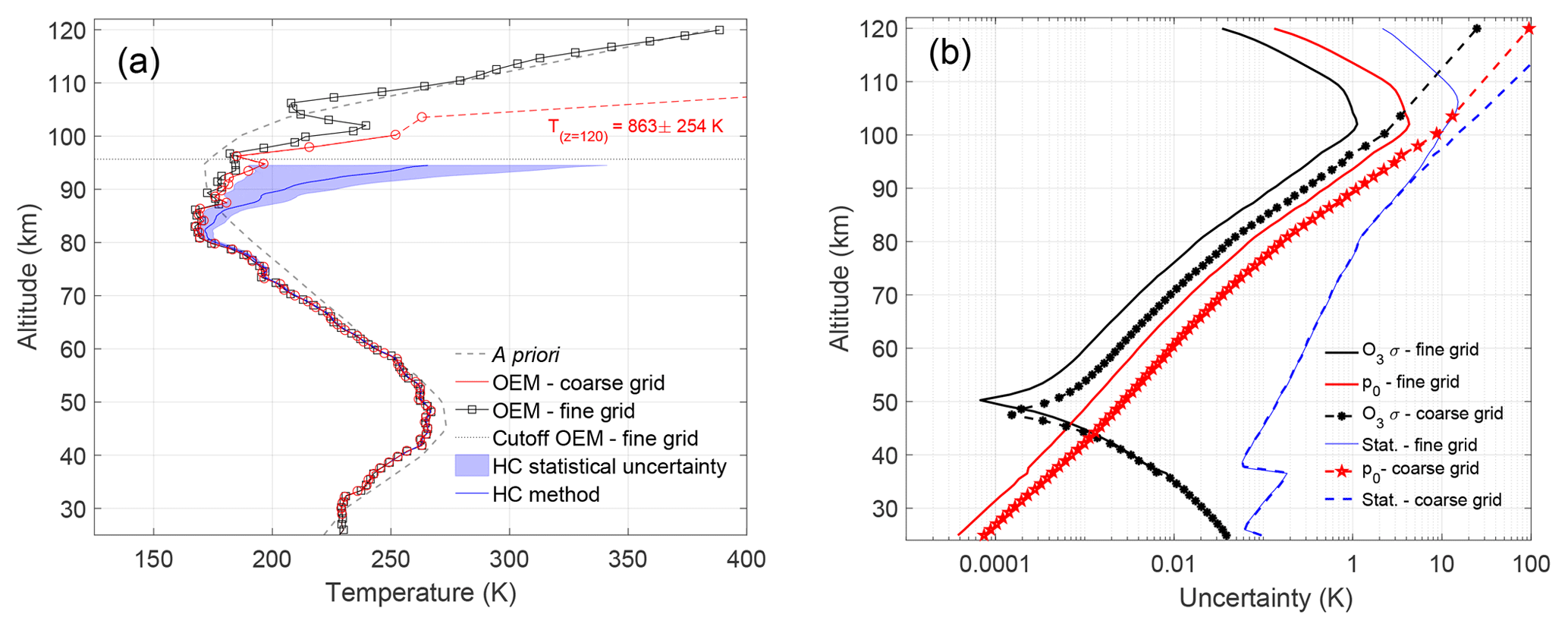
Figure 17(a) PCL temperature retrieval for the fine and coarse grids on 12 May 2012. The temperature and its uncertainty for the last coarse-grid point has a large value and it is not shown. (b) The statistical and systematic uncertainties due to the tie-on pressure and ozone cross section for the PCL temperature retrieval. The other systematic uncertainty terms included in our retrieval are not shown.
Figure 17a shows the OEM fine- and ML coarse-grid temperature retrievals compared to the Chanin and Hauchecorne (HC) temperature calculation (Hauchecorne and Chanin, 1980). The two OEM and ML retrievals are identical up to 88 km. Above 88 km the coarse-grid retrieval differs from the fine-grid retrieval and provides only four additional levels. The last two levels are shown with dashed lines in Fig. 17a and are points that we would not consider in the retrieval due to their large uncertainties. The last meaningful point shown in Figure 17a is around 100 km, where the corresponding statistical uncertainty is 15 K and the systematic uncertainties due to the tie-on pressure and ozone cross section are 9 and 2.3 K, respectively. Therefore, the last valid point of the retrieved temperature on the fine grid is within the total uncertainty of the coarse grid, and the final retrieval altitude increases by 4 km.
In this case, it cannot be concluded if the HC result is closer to the fine- or coarse-grid result. In order to investigate, we used nine additional nights randomly picked from PCL measurements, and the percent difference between the fine- and coarse-grid retrieval with the HC method was calculated (Fig. 18). In general, the method does just as well as the regular OEM, or better, with respect to the HC method results. We may also conclude that, in general, the a priori temperatures do not have a large effect on the profiles retrieved with the OEM for most nights; however, for nights such as 24 and 28 May 2012 the a priori information seems to have had a larger effect which is removed by our technique.
A consequence of applying this method is that the uncertainties in the retrieval increase where the coarse grid is not equal to the fine grid. Figure 17b shows the statistical uncertainty on the fine and coarse grid, as well as two of the largest systematic uncertainties, including the uncertainty in the retrieved temperature due to the tie-on pressure and ozone cross section. The most sensitive uncertainty parameter is the statistical uncertainty, which changes from 13 to 20 K at 98 km. The details of the systematic uncertainties on the fine grid are discussed in Sica and Haefele (2015) and Jalali et al. (2018). The systematic uncertainties increase after a priori removal due to the gain matrix (Eq. 5) increasing after the regularization term is removed. In general, all uncertainties on the coarse grid (Fig. 17b) increase at higher altitudes, where contribution from the a priori temperature profile starts. The increasing of the random uncertainties at the highest altitudes is due to decreasing photo counts from the exponential decrease in air density.
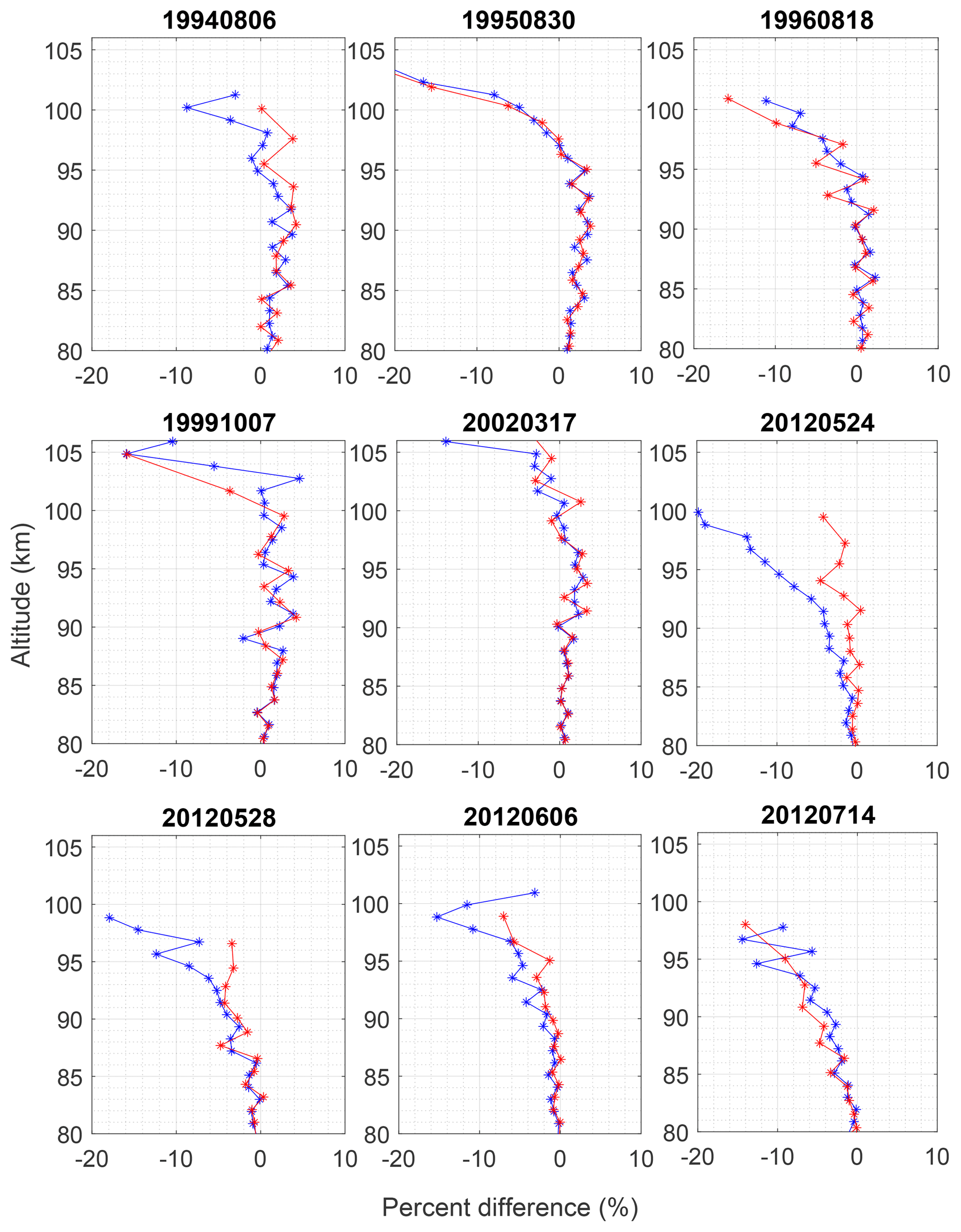
Figure 18The percent difference between the fine-grid retrieval with the HC method (blue line) and coarse-grid retrieval (a priori removed) with the HC method (red line). Below 80 km the retrievals are identical, as the coarse and fine grid are identical.
To illustrate that the a priori information is in fact being removed, we compared the temperature retrievals using two very different a priori temperature profiles, one calculated by CIRA-86 and one calculated by the US Standard Atmosphere (Fig. 19). The difference between the two temperatures on the fine-grid retrieval is shown by the black curve and is about 2 K at the 0.9 cutoff line, within the statistical uncertainty. The difference increases rapidly above that height. The same temperature difference after the a priori information is removed is shown in red and is on the order of 0 at all altitudes.
The HC method considers the fact that the atmosphere consists of isothermal layers and uses a seed pressure (or temperature) at the top of each measurement profile to calculate the temperature in the lower layers. The maximum height at which there is enough information in the signal is at SNR equals 2. Therefore, the seed value usually is chosen at the altitude that the SNR of 2 and 10 km from the top of the temperature profile is removed due to the seed value uncertainty. We also examined the relationship with the Rayleigh temperature retrieval and the SNR of the Rayleigh channel signal to determine if there was a similarly consistent value associated with the measurement response cutoff height as there was for the water vapor retrievals. However, based on the examination of all 500+ nights in the Jalali et al. (2018) study, removing 10 km below the altitude at which the SNR =2 yields cutoff altitudes higher than the measurement response of 0.8, which suggests that removing 15 km instead of 10 km may be more consistent with the OEM technique.
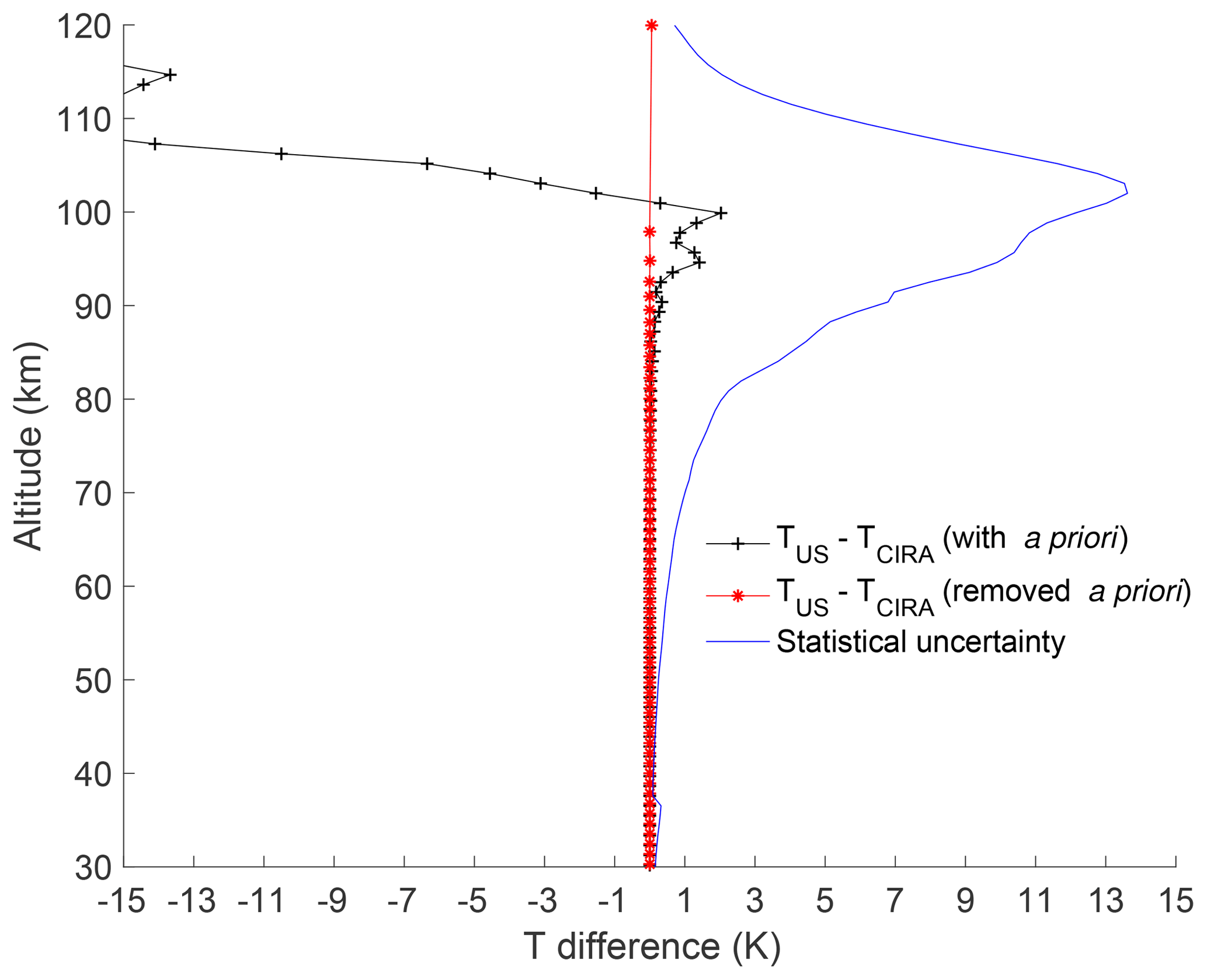
Figure 19PCL temperature difference between the OEM retrieved temperature profiles using values from the US Standard Atmosphere and CIRA-86 as the a priori temperature profiles.
We have developed a method to remove the influence of the a priori temperature and water vapor profiles on the retrieval based on the method discussed in vCG. These authors presented a method to re-regularize the retrieval in a way that the original a priori information is removed and the regularization on the fine grid emulates a coarser grid. These re-regularized profiles can then be resampled on a coarse grid without additional loss of information. The optimal coarse grid is determined from the averaging kernel matrix of the original retrieval. This method effectively removes the prior information from the retrieval while keeping the retrieval stable by the use of the coarser final grid. This independence of a priori information can be diagnosed by the averaging kernel matrix, which is unity on the coarse grid.
vCG presented two approaches, a “staircase” representation and a “triangular” representation, to transform the retrieval from the fine to the coarse grid. The cumulative trace of A shows the total degrees of freedom of the retrieval. In these representations, the cumulative trace of the averaging kernel matrix A as a function of altitude is calculated and is then interpolated to the coarse grid based on the centered information approach. As each space contains only one degree of freedom, the spaces are distributed. The staircase representation with its discontinuities at the layer boundaries is not a realistic representation of the atmosphere; therefore we use the triangular representation here to create the coarse grid. In the triangular representation, the highest and lowest level of the coarse grid are considered to be the same as the fine grid, and the rest of the grid points are distributed such that each layer between two levels represents approximately one degree of freedom.
Our method differs from vCG in that we do not re-regularize the retrieval to remove the a priori information. Instead, after the initial retrieval, we remove the regularization term from the retrieval and rerun the retrieval using the coarse grid. This second run of the retrieval is then equivalent to a maximum likelihood retrieval whose results are solely based on the information provided by the measurements. Both the proposed method and that of vCG are equally effective; however, our method is more of a brute-force technique but easier to practically implement since it is trivial to rerun the retrieval a second time.
For lidars, the triangular coarse-grid calculation results in a grid that is very close to the original OEM retrieval at the lower retrieval altitudes where there is more signal and the averaging kernels of the OEM are close to unity. However, at higher altitudes, where the OEM averaging kernels decrease, the information is spread over more altitudes, and therefore the coarse-grid spacing becomes larger to compensate for the lack of information. An information-centered regridding approach is important for a ML retrieval because it is not guaranteed that any inhomogeneous grid will produce a stable a priori-free retrieval. Additionally, a statistical gridding approach is easily automated and creates a grid that represents the physical conditions of the atmosphere.
We have shown how the a priori removal method works for three sample retrievals: water vapor during both daytime and nighttime, and a nighttime Rayleigh temperature. The a priori removal technique is most useful when the SNR is low, such as for daytime water vapor measurements. The method can increase the daytime retrieval altitude by up to 2 km, which is highly beneficial for meteorological studies that rely on accurate tropospheric measurements. The nighttime water vapor retrieval was provided for contrast to illustrate how the a priori removal technique does not provide significantly more information when the signal level falls off rapidly.
For Rayleigh temperature retrievals, we used measurements from the PCL in London, Ontario. Jalali et al. (2018) suggested that the 0.9 level be used as the valid cutoff height. In the case of the PCL, we see that the second-to-last point on the coarse grid has a vertical resolution not much larger than the fine-grid retrieval (Fig. 16) and is very close to the same height; therefore, the 0.9 measurement response value seems to be a conservative choice for a valid cutoff. We also showed that the effect of the a priori is removed completely in the Rayleigh temperature retrieval when we compared the differences in the retrieved temperature using the values from CIRA-86 and from the US Standard Atmosphere as the a priori profiles (Fig. 19). The presented method provides us with higher altitudes for the retrieved temperature profiles. Additionally, where the retrieved temperature profile in the coarse grid is the same as it is for the fine grid, we can be confident the temperature retrieval has a negligible contribution from the chosen a priori temperature profile.
An advantage of our method over OEM is that the entire coarse-grid profile is a priori-free, in the sense that the regularization term does not contribute to the retrieval. In regions where the SNR is low or the averaging kernel is significantly less than 1, the a priori removal method improves the validity of the retrieval. An a priori-free profile is especially useful for trend analyses and climatological studies which must not include prior information and must be wholly based on measurements. The advantage of an information-centered grid for a typical measurement may be used for multiple retrievals. A grid which is optimal for one atmospheric state will in most cases be close to optimal for a similar atmospheric state. With this consistent grid choice, the altitude resolution of a multiyear time series will be consistent, which is important when working with data over long time periods or conducting trend analyses. Varying information content of the individual measurements will lead to error bars of different size. The coarse grid allows time series analysis or trend analysis for single altitudes without problems caused by varying vertical resolution.
The important trade-off with this technique is that the uncertainties of the retrieval increase when moving from an OEM fine-grid retrieval to a ML coarse-grid retrieval. Both the systematic and statistical uncertainties in the second ML retrieval increase due to the removal of the inverse of the a priori covariance matrix from the gain equation (Eq. 5). The vertical resolution of the profile also increases as a consequence of the method. We also lose the ability to determine the maximum useful retrieval altitude by using the averaging kernels. In this case, it is necessary to use the uncertainties to determine the maximum altitude. While the a priori removal gives us more confidence in the retrieval, we may not consider the entire profile meaningful due to high uncertainties. Hence, the last few points with unity averaging kernel value on the coarse grid may not be recognized as valid retrieval levels.
We have developed a practical and robust method which removes the effect of a priori information in lidar OEM retrievals. The method utilizes an information-centered coarse grid which is derived using the averaging kernels from the initial fine-grid retrieval. The resulting coarse grid is then used, alongside setting the inverse of the a priori covariance matrix to zero, to create the final ML retrieval without any a priori information. The method has little computational cost; the OEM retrieval is extremely fast even on a laptop computer, so having to do the retrieval twice for each profile is not critical. We illustrated the method using a simple example in Sect. 4 and demonstrated the removal method using the water vapor signal from the RALMO and the Rayleigh temperature signal from the PCL. We summarize the results from both of these examples as follows.
-
Figure 1b shows that 90 % of the nights in the temperature climatology from Jalali et al. (2018) had less than a 5 K influence from the a priori temperature profiles at the Au=0.9 cutoff height. Additionally, in all cases the a priori temperature influence was less than the statistical uncertainty, as was illustrated in Fig. 6 in Jalali et al. (2018). Although small, the a priori temperature profile does contribute to the retrieved temperature in regions where the measurement response is smaller than 1.
-
The a priori removal technique increased the maximum altitude of the water vapor daytime retrieval by an average of 1 km and up to a maximum of 2 km; however, the maximum altitude is on the same order of the fine-grid retrieval height if a lower uncertainty threshold is adopted. Both OEM fine-grid and ML coarse-grid retrievals produced similar differences with respect to the radiosonde which agreed within their respective uncertainties (Fig. 6). While the nighttime coarse-grid retrievals did not show a significant increase in cutoff height, they did increase on average by a few hundred meters. The nighttime water vapor averaging kernels decrease quickly with height and therefore have very little information to add to the retrieval, thereby resulting in very small increases in altitude when using the coarse grid.
-
Applying the method to the PCL temperature retrieval showed useful retrievals above the Au=0.9 cutoff height by 2 km, validating the choice of Au=0.9 for a cutoff made in Jalali et al. (2018) to form their climatology up to an altitude where tie-on pressure effects were minimal. The temperatures below the cutoff height were the same.
-
In all cases, the vertical resolution of the OEM retrieval decreases after a priori removal.
-
The systematic uncertainties after a priori removal increase roughly by a factor of 2 but remain on the same order of magnitude as before the a priori removal. The values of the systematic uncertainties also remain significantly smaller than the statistical uncertainties.
-
The temperature difference between the PCL retrieved temperature profiles using two different a priori profiles was used to show the effectiveness of the a priori removal method. The temperature difference before removal around the 0.9 cutoff height was more than 2 K; however, this value was zero for the entire range after a priori removal.
-
The water vapor measurement response values of 0.9 consistently corresponded to a SNR of 2 for the nighttime retrievals and between 1 and 2 for the daytime retrievals. Therefore, it is our recommendation that traditional water vapor retrievals be cut at a SNR of 2 to compare with the OEM water vapor retrievals. Additionally, measurement response values of 0.8 or higher corresponded to SNR values of 1 or less than 1; therefore we would not suggest cutting the water vapor retrievals at heights above which the measurement response is less than 0.9.
-
The Rayleigh temperature measurement response 0.9 cutoff height was also compared to the SNR of the Rayleigh signal. However, no correlation could be found between the cutoff height and the SNR value. In fact, removing 10 km below a SNR of 2 tended to correspond to measurement response values of less than 0.8, which suggests that it may be more appropriate to remove 15 km from the altitude at which the SNR equals 2 to achieve results more consistent with the OEM.
When designing an OEM retrieval, it is often desirable to understand the effect of the chosen a priori parameters or profiles. This effect has been explored in detail for satellite-based and passive ground-based instruments but not for the new area of applying OEM to active-sensing measurements such as lidar. Lidars are high-resolution instruments with significant amounts of information available from their measurements, as evidenced by the retrieval averaging kernels. The OEM helps to illustrate the robustness of the lidar data products with the advantage of providing diagnostic tools, such as the averaging kernel and a full uncertainty budget.
The a priori removal technique may be helpful for checking the a priori's influence on the retrieval and in determining the appropriate a priori. It is also important to note that the differences between the fine-grid OEM retrieval and the coarse-grid ML retrieval may be smaller if one uses an a priori closer to the true atmospheric state. Often, reanalysis model profiles are used as a priori for OEM retrievals because they are closer to the atmospheric true state than a climatological profile. However, the nature of the a priori profile should depend on the design of the instrument and the goal of the work.
In this study, the US Standard Atmosphere water vapor profile was chosen as the a priori profile to accommodate the operational nature of RALMO lidar water vapor measurements, which requires a minimal number of dependencies in the code as possible and preferably no need for internet. The CIRA temperature profile was used for the temperature a priori because there are very few model temperature a priori profiles above 80 km for the PCL and coincident satellite measurements are not always available. Additionally, when conducting trend analyses or climatological studies it may be more useful to use a consistent a priori profile throughout the analysis to avoid inducing trends or biases into the results.
The removal method is most operationally useful for lidar measurements with low signal to noise and a slow transition from regions of high signal to low signal. The method is less effective at increasing the maximum retrieval altitude when signal strength changes rapidly, such as when the nighttime water vapor measurements quickly enter the dry upper troposphere or lower stratosphere. However, the method is most useful for homogenizing large data sets for trend analyses. One representative coarse grid would be applied to an entire data set and a ML retrieval would be run to remove a priori information from all measurements, thereby making them suitable for trends.
In the future, this method will be applied to the entire 10 years of RALMO measurements to retrieve the water vapor daytime and nighttime measurements and create a water vapor climatology. We anticipate that this technique will increase the altitude of the daytime water vapor retrievals by several kilometers. It is also our hope that this method may provide statistically significant measurements in the UTLS region. Finally, the RALMO water vapor climatology will be used to find trends.
RALMO data are available upon request from Alexander Haefele by email: alexander.haefele@meteoswiss.ch. PCL data are available upon request from Robert J. Sica by email: sica@uwo.ca. GRUAN radiosonde data from Payerne can be downloaded via the GRUAN website (http://www.gruan.org, GRUAN, 2019).
AJ was responsible for developing the a priori removal method and code as well as manuscript preparation, including the following sections: Introduction, Theoretical background, Methodology, Purple Crow Lidar Rayleigh temperature a priori removal, Summary, Discussion, and Conclusions. He also applied the method to the Rayleigh temperature analysis. This work is the second component of his doctoral thesis. SHJ applied the removal method to the water vapor daytime and nighttime analyses as well as helped with manuscript preparation, including the following sections: Introduction, Theoretical background, Methodology, Daytime RALMO water vapor a priori removal, Nighttime RALMO water vapor a priori removal, Summary, Discussion, and Conclusions. This will serve as a component of her doctoral thesis. RJS was responsible for supervising the doctoral theses and contributed to manuscript preparation. AH was also responsible for supervising the doctoral thesis of SHJ and contributed to manuscript preparation and scientific discussions. TvC significantly contributed to the scientific discussions which resulted in this paper, helped develop the method based on his original work, and contributed to manuscript preparation.
The authors declare that they have no conflict of interest.
We would like to thank the Federal Office of Meteorology and Climatology, MeteoSwiss, for its support of this project and providing the water vapor lidar measurements. We would like to thank the GRUAN support team for providing the GRUAN-processed radiosonde measurements.
This project has been funded in part by the National Science and Engineering Research Council of Canada through a Discovery Grant (Sica) and a CREATE award for a Training Program in Arctic Atmospheric Science (Dr. Kim Strong, PI), as well as by MeteoSwiss (Switzerland).
This paper was edited by Andrew Sayer and reviewed by three anonymous referees.
Boersma, K. F., Eskes, H. J., and Brinksma, E. J.: Error analysis for tropospheric NO2 retrieval from space, J. Geophys. Res., 109, D04311, https://doi.org/10.1029/2003JD003962, 2004. a
Brocard, E., Philipona, R., Haefele, A., Romanens, G., Mueller, A., Ruffieux, D., Simeonov, V., and Calpini, B.: Raman Lidar for Meteorological Observations, RALMO – Part 2: Validation of water vapor measurements, Atmos. Meas. Tech., 6, 1347–1358, https://doi.org/10.5194/amt-6-1347-2013, 2013. a
Ceccherini, S., Raspollini, P., and Carli, B.: Optimal use of the information provided by indirect measurements of atmospheric vertical profiles, Opt. Express, 17, 4944–4958, https://doi.org/10.1364/OE.17.004944, 2009. a
Committee on Extension to the Standard Atmosphere: U.S. standard atmosphere, US Government Printing Office, 1–227, NASA-TM-X-74335, NOAA-S/T-76-1562, 1976. a
Cunnold, D. M., Chu, W., Barnes, R. A., McCormick, M. P., and Veiga, R. E.: Validation of SAGE II ozone measurements, J. Geophys. Res., 94, 8447–8460, https://doi.org/10.1029/JD094iD06p08447, 1989. a
Dinoev, T., Simeonov, V., Arshinov, Y., Bobrovnikov, S., Ristori, P., Calpini, B., Parlange, M., and van den Bergh, H.: Raman Lidar for Meteorological Observations, RALMO – Part 1: Instrument description, Atmos. Meas. Tech., 6, 1329–1346, https://doi.org/10.5194/amt-6-1329-2013, 2013. a
Dirksen, R. J., Sommer, M., Immler, F. J., Hurst, D. F., Kivi, R., and Vömel, H.: Reference quality upper-air measurements: GRUAN data processing for the Vaisala RS92 radiosonde, Atmos. Meas. Tech., 7, 4463–4490, https://doi.org/10.5194/amt-7-4463-2014, 2014. a
Fleming, E. L., Chandra, S., Shoeberl, M. R., and Barnett, J. J.: Monthly Mean Global Climatology of Temperature, Wind, Geopotential Height and Pressure for 0–120 km, NASA Tech. Memo, NASA TM100697, 85 pp., 1988. a
GRUAN: GCOS Reference Upper Air Network, available at: http://www.gruan.org, last access: 13 July 2019. a
Hauchecorne, A. and Chanin, M.: Density and temperature profiles obtained by lidar between 35 and 70 km, Geophys. Res. Lett., 7, 565–568, https://doi.org/10.1029/GL007i008p00565, 1980. a
Hyland, R. and Wexler, A.: Formulations for the thermodynamic properties of the saturated phases of H2O from 173.15 K to 473.15 K, ASHRAE Tran., 89, 500–519, 1983. a
Jalali, A., Sica, R. J., and Haefele, A.: Improvements to a long-term Rayleigh-scatter lidar temperature climatology by using an optimal estimation method, Atmos. Meas. Tech., 11, 6043–6058, https://doi.org/10.5194/amt-11-6043-2018, 2018. a, b, c, d, e, f, g, h, i, j, k, l, m, n
Joiner, J. and Silva, A. D.: Efficient methods to assimilate remotely sensed data based on information content, Q. J. Roy. Meteor. Soc., 124, 1669–1694, https://doi.org/10.1002/qj.49712454915, 1998. a
Povey, A. C., Grainger, R. G., Peters, D. M., and Agnew, J. L.: Retrieval of aerosol backscatter, extinction, and lidar ratio from Raman lidar with optimal estimation, Atmos. Meas. Tech., 7, 757–776, https://doi.org/10.5194/amt-7-757-2014, 2014. a
Rodgers, C. D.: Retrieval of atmospheric temperature and composition from remote measurements of thermal radiation, Rev. Geophys., 14, 609–624, https://doi.org/10.1029/RG014i004p00609, 1976. a
Rodgers, C. D.: Inverse Methods for Atmospheric Sounding: Theory and Practice, vol. 2, World Scientific, Hackensack, NJ, USA, https://doi.org/10.1142/3171, 2000. a, b, c, d
Sica, R. J. and Haefele, A.: Retrieval of temperature from a multiple-channel Rayleigh-scatter lidar using an optimal estimation method, Appl. Optics, 54, 1872–1889, https://doi.org/10.1364/AO.54.001872, 2015. a, b, c, d, e, f, g
Sica, R. J. and Haefele, A.: Retrieval of water vapor mixing ratio from a multiple channel Raman-scatter lidar using an optimal estimation method, Appl. Optics, 55, 763–777, https://doi.org/10.1364/AO.55.000763, 2016. a, b, c, d
Vincent, R. A., Dudhia, A., and Ventress, L. J.: Vertical level selection for temperature and trace gas profile retrievals using IASI, Atmos. Meas. Tech., 8, 2359–2369, https://doi.org/10.5194/amt-8-2359-2015, 2015. a
von Clarmann, T. and Grabowski, U.: Elimination of hidden a priori information from remotely sensed profile data, Atmos. Chem. Phys., 7, 397–408, https://doi.org/10.5194/acp-7-397-2007, 2007. a, b