the Creative Commons Attribution 4.0 License.
the Creative Commons Attribution 4.0 License.
 | 19 Jul 2019
Comparison between the assimilation of IASI Level 2 ozone retrievals and Level 1 radiances in a chemical transport model
Emanuele Emili
Brice Barret
Eric Le Flochmoën
Daniel Cariolle
The prior information used for Level 2 (L2) retrievals in the thermal infrared can influence the quality of the retrievals themselves and, therefore, their further assimilation in atmospheric composition models. In this study we evaluate the differences between assimilating L2 ozone profiles and Level 1 (L1) radiances from the Infrared Atmospheric Sounding Interferometer (IASI). We minimized potential differences between the two approaches by employing the same radiative transfer code (Radiative Transfer for TOVS, RTTOV) and a very similar setup for both the L2 retrievals (1D-Var) and the L1 assimilation (3D-Var). We computed hourly 3D-Var analyses assimilating L1 and L2 data in the chemical transport model MOCAGE and compared the resulting O3 fields among each other and against ozonesondes. We also evaluated the joint assimilation of limb measurements from the Microwave Limb Sounder (MLS) in combination with IASI to assess the impact of stratospheric O3 on tropospheric analyses. Results indicate that significant differences can arise between L2 and L1 assimilation, especially in regions where the L2 prior information is strongly biased (at low latitudes in this study). In these regions the L1 assimilation provides a better variability of the free-troposphere ozone column. L1 and L2 assimilation instead give very similar results at high latitudes, especially when MLS measurements are used to constrain the stratospheric O3 column. A critical analysis of the potential benefits and drawbacks of L1 assimilation is given in the conclusions. We also list remaining issues that are common to both the L1 and L2 approaches and that deserve further research.


The global monitoring of atmospheric composition relies on a large number of dedicated satellite missions and on the sustained improvement of numerical forecast models. Today, research and operational centres provide both satellite-based reanalyses and forecasts of atmospheric composition for a large number of applications, spanning from stratospheric ozone monitoring (van der A et al., 2010) to climate change (Flemming et al., 2017) and air quality (Zhang et al., 2012; Marécal et al., 2015).
Satellite sensors measure the spectral signature of gases and aerosols on the radiation field that traverse the atmosphere. Retrieving the concentration of a given gas from the radiation measured at the satellite position represents an inverse problem that is in most cases ill-posed and underdetermined; i.e. finding the solution requires some type of mathematical regularization or prior information (Rodgers, 2000). The accuracy of the solution depends in general on the intensity of the spectral signature of the retrieved compound, the source of radiation (e.g. the Earth or the Sun), the observation geometry and the accuracy of the radiative transfer model (RTM). The last-mentioned factor also means correctly accounting for all the atmospheric constituents or surface properties that affect the radiation field but are not retrieved themselves (auxiliary RTM inputs).
When the retrieval is done within a Bayesian framework, like the optimal estimation method (Rodgers, 2000), the measurement errors, the RTM errors and the uncertainty in the prior information (also named background or a priori profile) are prescribed. The procedure then provides an estimation of the error covariance for the retrieved quantity and the averaging kernels (AKs), which quantify the sensitivity of the retrieval to the true state and are linked to the degrees of freedom (DOF) of the solution. The retrieval errors and the AKs (or the DOF) can be used first to diagnose the quality and the relevance of the atmospheric retrieval. They become even more important when retrievals are further assimilated in numerical forecast models because they weight the impact of the observations in the system.
Chemical transport models (CTMs) solve the chemical and physical processes within the atmosphere but are based on meteorological fields from a numerical weather prediction (NWP) model to advect the chemical species. Coupled chemistry–meteorology models (CCMMs) that simulate both meteorology and chemistry online became available later but are quite common today in operational centres (Zhang et al., 2008; Flemming et al., 2015). There are currently growing efforts to introduce even stronger coupling of the atmosphere with both ocean and surface models, which has given rise to so-called Earth system models (ESMs; Brown et al., 2012; Hurrell et al., 2013). ESMs provide a comprehensive tool for climate predictions and reanalyses, but they are also considered for state-of-the-art air-quality modelling (Neal et al., 2017).
Closely following the historical advances in modelling, the assimilation of satellite data was first introduced in CTMs (Geer et al., 2006; Lahoz et al., 2007), and it is now also well integrated in operational CCMMs (Flemming et al., 2017).
Today, numerous satellite retrievals of trace gases (e.g. O3, CO, NO2, CH4, CO2) and aerosols (aerosol optical depth, AOD) are assimilated daily within operational CTMs and CCMMs (Inness et al., 2015; Bocquet et al., 2015).
For a long time, meteorological variables such as temperature and water vapour profiles have been corrected by means of assimilating satellite radiances (Level 1 data) directly in NWP models. Therefore, the RTM became part of the observation operator of the assimilation system (Andersson et al., 1994). This avoided the introduction of biases in NWP that arose from poor prior information used in satellite retrievals at that time and neglect of the AKs (Eyre et al., 1993). On the other hand, chemical species and aerosols are mostly corrected by means of assimilating geophysical retrievals (Level 2 or L2 data) that are made available by satellite data providers. To remove the impact of the prior information when assimilating L2 retrievals, the AK of the retrieval must be multiplied by the modelled profiles before computing the innovation vectors (Rodgers, 2000; Eskes and Boersma, 2003; Migliorini, 2012). However, within standard methods based on the linearization of the RTM, like optimal estimation, issues might still arise when the prior information used in the retrieval is far from the true atmospheric state: this might challenge the linearization of the observation operator and result in sub-optimal retrievals. Since the AKs themselves are also a result of the retrieval (and depend upon its prior information), we expect that a perfect removal of the prior information within data assimilation (DA) cannot always be ensured.
The precise conditions that provide an equivalence between assimilating retrievals (using some kind of weighting function) and radiances have been formalized by Migliorini (2012) and further tested by Prates et al. (2016) on synthetic satellite observations. These authors conclude that the equivalence holds under the hypothesis of an almost linear radiative transfer (RT) regime and with careful selection of the prior error covariances in order to maximize the measurement information in the retrieval step. Nonetheless, testing the two approaches within an operational system and with real observations remains crucial to verify whether these conditions are met in practice. Moreover, the perfect equivalence only holds when all the auxiliary inputs of the RTM are exactly the same in both the retrieval and the radiance assimilation. It is clear that a climatological option for some RTM inputs will always be a more practical choice when computing L2 retrievals. On the other hand, the evolution towards strongly integrated ESMs will allow in principle to dispose of the most accurate prior information for all RTM inputs and favours the radiance assimilation approach. In this context, it appears important to introduce and evaluate the assimilation of radiances for chemical applications as well.
To the best of the authors' knowledge, the existent literature on this topic only concerns meteorological applications. Han and McNally (2010) explored the possibility of assimilating O3 sensitive radiances within a NWP model but without comparing the two approaches. Similarly, Weaver et al. (2007) examined the assimilation of satellite radiances for aerosols, but the focus was on the impact of using modelled aerosol microphysical properties as auxiliary input for the RTM, and no comparison was provided. No other studies could be found concerning the assimilation of chemical compounds.
The objective of this study is to perform a first strict comparison between the assimilation of radiances and retrievals, with respect to O3 estimation in the thermal infrared (TIR). To this end, systematic differences between the assimilation of retrieval and radiances have been minimized as much as possible, for example by means of employing the same RTM within the two approaches.
We consider the case of O3 assimilation using the Infrared Atmospheric Sounding Interferometer (IASI) on board the European MetOp satellites (Clerbaux et al., 2009). Several IASI O3 retrievals have already been well validated (Dufour et al., 2012) and used directly to provide multi-annual time series of the global O3 budget (Wespes et al., 2016) or successfully assimilated within global (Peiro et al., 2018) and regional CTMs (Coman et al., 2012). However, an empirical correction of the retrievals has been found to be necessary to ensure globally unbiased reanalyses, and slightly degraded assimilation results are still found at mid-latitudes and high latitudes (Emili et al., 2014). Since the tropospheric O3 signature in the selected IASI spectral window decreases over colder surfaces, the impact of the retrieval's prior information might become more relevant at high latitudes. In addition, the majority of IASI O3 retrievals use a single a priori profile globally (Barret et al., 2011; Boynard et al., 2016), which might present very large local departures from the true O3 profile. Hence, IASI O3 assimilation represents a good benchmark to evaluate the differences between the assimilation of retrievals and radiances.
The IASI SOFRID (Software for a Fast Retrieval of IASI Data) O3 product (Barret et al., 2011) and MOCAGE CTM have been used here to benefit from the experience of previous studies (Emili et al., 2014; Peiro et al., 2018). SOFRID and MOCAGE DA are based on a variational algorithm, and, since SOFRID employs RTTOV (Saunders et al., 1999), which is a community RTM developed originally for NWP applications, the same RTM has been implemented in the MOCAGE system. Global O3 analyses are computed for July 2010, and the results are compared against all available radiosoundings to evaluate their accuracy. Since the sensitivity of IASI TIR measurements to O3 is not uniform along the atmospheric column, we also investigate the impact of assimilating more accurate stratospheric profiles from the Microwave Limb Sounder (MLS) in combination with IASI radiances. This might reveal possible synergies when assimilating multiple instruments that sense different layers of the atmosphere.
The paper is organized as follows. The satellite measurements, the Level 2 retrievals and the validation measurements used for this study are described in Sect. 2, as well as main steps concerning the preprocessing for some of the datasets. The chemical transport model, the radiative transfer model, the assimilation algorithm and the setup of the experiments are described in Sect. 3. The assimilation of IASI retrievals and radiances is compared in Sect. 4.1, and the impact of MLS assimilation in combination with IASI is discussed in Sect. 4.3. The conclusions are summarized in the last section, where some recommendations are also given.
2.1 IASI
IASI flies on board the series of polar-orbiting satellites MetOp operated by the EUropean organization for the exploitation of METeorological SATellites (EUMETSAT). It provides hyper-spectral measurements of the Earth's thermal radiation in the 3.62–15.5 µm (2760–645 cm−1) window and serves meteorological and atmospheric chemistry applications (Clerbaux et al., 2009; Hilton et al., 2012). IASI is an operational mission meant to provide long-term (>20 years) time series of accurate TIR spectra at high spatial resolution. A total of three IASI instruments will be flying simultaneously at the end of 2019, providing nearly global coverage six times per day (morning and evening overpasses). Hence, they represent a great opportunity for both NWP and climate–chemistry reanalyses. Only MetOp-A data, available from 2008 to present, have been employed for this study.
2.1.1 L1 radiances
IASI L1c data contain calibrated and geolocalized spectra at 0.5 cm−1 spectral resolution (after apodization), i.e. 8461 radiance values for each ground pixel, with a footprint of 12 km for nadir observations. For this study, historical L1c data granules have been downloaded from the EUMETSAT Earth Observation data portal (https://eoportal.eumetsat.int, last access: 16 July 2019) in NETCDF format. Data files also contain the observation geometry (Sun and satellite angles) for each ground pixel and the co-located land mask and cloud fraction values, obtained from the Advanced Very High Resolution Radiometer (AVHRR) measurements, also on board MetOp.
2.1.2 SOFRID L2 retrievals
The Software for a Fast Retrieval of IASI Data (SOFRID) was developed at the Laboratoire d'Aérologie to retrieve O3 (Barret et al., 2011) and CO (De Wachter et al., 2012) profiles from IASI. It is based on the Radiative Transfer for TOVS (RTTOV) RTM (Saunders et al., 1999) and the 1D-VAR scheme developed within the Numerical Weather Prediction Satellite Application Facilities (NWP SAF) programme. SOFRID retrieves the O3 profile in volume mixing ratio (vmr) units at 43 pressure levels between the surface and 0.1 hPa using 469 spectral channels within the main IASI O3 window (980–1100 cm−1). The choices that are made in SOFRID and are relevant for this study are summarized in Table 2. Note that a single a priori profile and error covariance matrix are used globally and that the surface skin temperature (SST) is estimated within the retrieval.
The number of DOF of the SOFRID retrieval has been evaluated to be between 2 and 3 for the full atmospheric column, with about 1 DOF for the tropospheric column (Dufour et al., 2012). SOFRID's averaging kernels corresponding to the retrievals used within this study (see Sect. 2.4) are shown in Fig. 1. We remark that the largest sensitivities are found for the lower stratosphere (50–100 hPa) and upper troposphere (200–300 hPa) levels. The sensitivity in the free troposphere (400–600 hPa) is maximum at tropical latitudes and decreases towards the poles due to the decreasing thermal contrast. Very low sensitivities are in general found for levels below 700 hPa at all latitudes.
(Borbas and Ruston, 2010)(Borbas and Ruston, 2010)Table 2Summary of the configuration of SOFRID L2 retrievals and MOCAGE L1 assimilation.

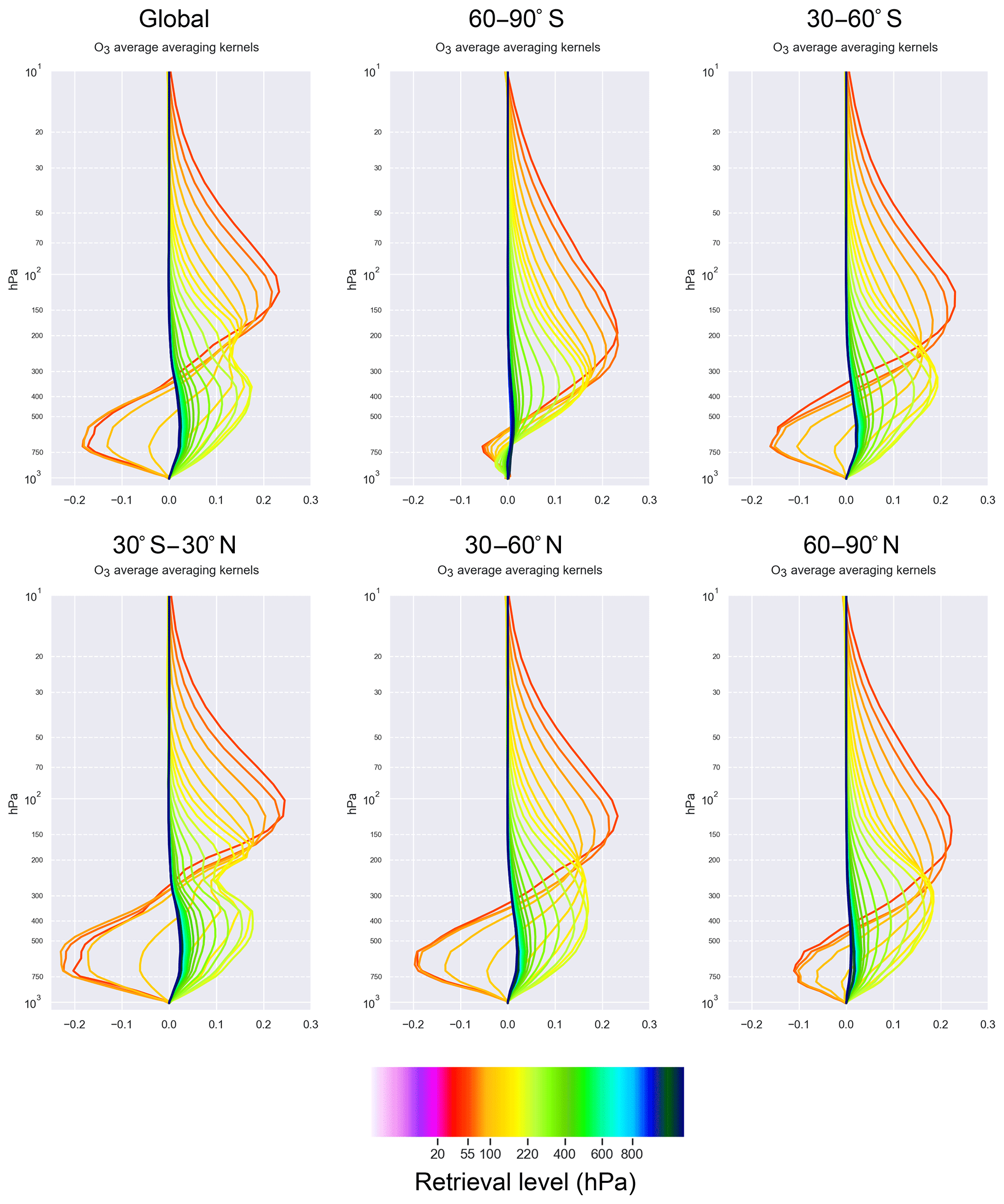
Figure 1SOFRID O3 averaging kernels for the month of July 2010 averaged globally (first plot) and for five separate latitude bands (90–60∘ S, 60–30∘ S, 30∘ S–30∘ N, 30–60∘ N, 60–90∘ N). Each coloured line corresponds to a retrieval's level, and the corresponding pressure is indicated in the colour bar. Only SOFRID levels with a pressure >50 hPa are displayed for better clarity.
The accuracy of the retrieved O3 depends on the latitude and the vertical level but is generally within 10 %–20 % of the corresponding radiosounding values, once the averaging kernels are applied. However, biases are found in the troposphere with SOFRID (+10 %), and positive biases of about 15 % are found in the upper troposphere–lower stratosphere (UTLS) region with all current IASI O3 products (Dufour et al., 2012). The reasons for such biases are not yet fully understood and can impact data assimilation (Emili et al., 2014) or trend analysis (Gaudel et al., 2018) negatively. This study will provide further insights about the impact of the constant a priori profile on IASI retrievals.
The SOFRID V1.5 retrievals described in Barret et al. (2011) are available for the full MetOp-A period at http://thredds.sedoo.fr/iasi-sofrid-o3-co (last access: 16 July 2019). The V3.0 version of SOFRID retrievals has been used for this study and was obtained from Brice Barret (personal communication, 2019). The main difference to version 1.5 concerns the temperature and water vapour profiles employed in the radiative transfer computations, which are taken from the ECMWF NWP model instead of EUMETSAT L2 retrievals. The SOFRID v3.0 preprocessor retrieves the operational analysis (type “an”) at 00:00, 06:00, 12:00, and 18:00 UTC from the ECMWF NWP model and assimilation system (Integrated Forecast System, IFS), regridded to a resolution of . All the fields are then interpolated at the closest hour to the IASI pixel, and a nearest-neighbour interpolation is done to extract the corresponding profiles and surface properties. Since the CTM is also based on ECMWF NWP forcing fields (Sect. 3.1), this choice minimizes possible systematic differences between L2 retrievals and L1 assimilation. Also, SOFRID v3.0 is based on a more recent version of RTTOV and newer IASI coefficients (v11.1, coefficients on 101 levels) than the original L2 product (v9.0, coefficients on 43 levels). In addition to the O3 retrieval and its error covariance, SOFRID files contain a number of auxiliary and diagnostic fields. The cloud fraction is based on a combination of the EUMETSAT L2 product (AVHRR) and a brightness temperature (BT) analysis at 11 and 12 µm to fill pixels with missing AVHRR data (Barret et al., 2011). An index based on the V-shaped sand signature computed as is used to detect pixels affected by large aerosol load. Usage of these products will be detailed in Sect. 2.4, “Data preprocessing”.
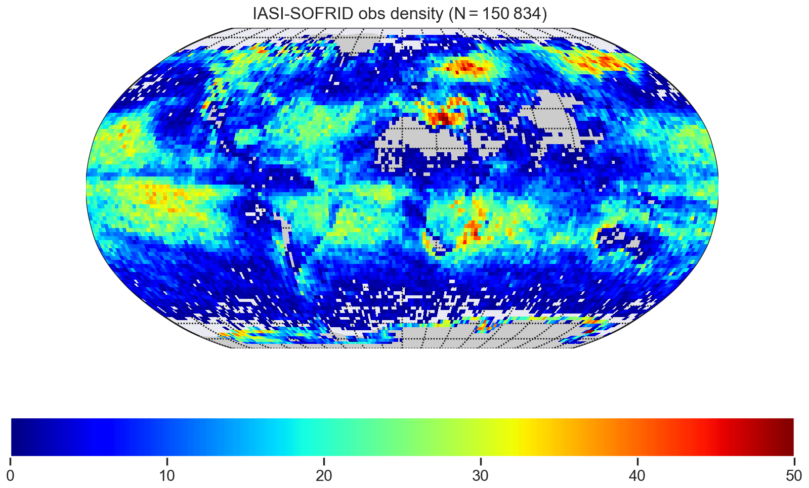
Figure 2Total number of IASI observations per model grid box () retained after the selection procedure described in Sect. 2.4 and further assimilated in this study for the month of July 2010. The total number of assimilated observation for the entire globe (N) is given above the map.
2.2 MLS L2 retrievals
Since 2004 the Microwave Limb Sounder (MLS) has been flying on board the research mission AURA and measures thermal emission at the atmospheric limb (Waters et al., 2006). It provides about 3500 stratospheric profiles of multiple atmospheric constituents each day, including O3 (Froidevaux et al., 2008). Since version 3 of MLS products has been in operation, O3 profiles have been retrieved on 55 pressure levels, with a recommended range for scientific usage between 0.02 and 261 hPa for version 4.2 (Livesey, 2018). The biases of MLS O3 profiles are typically within 5 % with respect to ozonesondes and lidar measurements (Hubert et al., 2016), with slightly higher values below 200 hPa. Given its good accuracy, MLS O3 has been widely used both for trend analysis (Froidevaux et al., 2015) and assimilation experiments (Massart et al., 2010; Miyazaki et al., 2012; Inness et al., 2015). Similarly to previous studies (Emili et al., 2014), we retain only the most accurate data using MLS, i.e. above 170 hPa. The MLS V4.2 product used in this study has been downloaded from the Goddard Earth Sciences Data and Information Services Center (GES DISC) web portal (https://disc.gsfc.nasa.gov, last access: 16 July 2019).
2.3 Radiosoundings
Ozonesondes are launched on a weekly basis by meteorological services and provide accurate profiles of O3 up to 10 hPa with a vertical resolution of 150–200 m. Electrochemical concentration cell (ECC) sondes, which represent the largest percentage of the global network, have a precision of about 5 % (Thompson et al., 2003). Radiosoundings are relatively sparse, and their geographical distribution is much more representative of the northern mid-latitudes. However, for several decades they have provided the most precise information on vertical ozone distribution in the troposphere. Therefore, they have been used to derive widely used tropospheric O3 climatologies (McPeters et al., 2007) and validate both satellite products (Dufour et al., 2012) or models (Geer et al., 2006). They will be used in this study to validate all model simulations. Data are collected and distributed by the World Ozone and Ultraviolet Radiation Data Center (WOUDC; http://www.woudc.org, last access: 16 July 2019).
2.4 Data preprocessing
Some further preprocessing has been applied to the original L1c and SOFRID datasets to ease the interpretation of the assimilation experiments presented later in Sect. 4. The objective was to ensure that exactly the same spectra are used for both L1 and L2 assimilation.
Only the spectral channels that are used in SOFRID are extracted from IASI L1c granules, i.e. channel no. 1350 (980 cm−1) to 1818 (1100 cm−1). Some further screening is applied to remove channels that are affected by strong H2O absorption, as also done in SOFRID.
The spatial resolution of the CTM (; Sect. 3.1) is much coarser than IASI pixel size. Since it is preferable to avoid all kind of spatial averaging of the observations, a significant reduction of ground pixels is needed. In return, we employ strict selection criteria to avoid contamination from clouds and bright surfaces as much as possible, which reduces the RT accuracy and increases retrieval or assimilation errors. The data selection is performed as follows.
First, only L1 pixels with both IASI and AVHRR highest-quality flags are kept.
Then, ground pixels from IASI L1 and SOFRID products are filtered using their respective cloud masks (Sect. 2.1.1 and 2.1.2) and only keeping pixels with a cloud fraction less than or equal to 1 %.
SOFRID pixels with a sand signature greater than 0.5 and with a number of retrieved levels lower than 35 (mountains) are also filtered out.
Resulting datasets are then matched; i.e. only common ground pixels that remained available after the previous L1 and SOFRID independent selections are kept. Finally, data thinning is performed using a regular grid of resolution and only keeping the first pixel that falls in every two grid boxes. This ensures a minimum distance of 1∘ among assimilated observations. After the completion of the data selection procedure the final number of retained ground pixels for L1 and SOFRID is about 5000 per day, compared to about 105 when only the cloud screening is applied. The total number of L1 and L2 observations resulting from the above selection and further assimilated in this study is displayed in Fig. 2.
This section summarizes the main characteristics of the CTM (Sect. 3.1), the RTM (Sect. 3.2) and the assimilation algorithm (Sect. 3.3) used in this study. Further details on the particular selection of the main parameters of the assimilation experiments (e.g. the error covariances) are given in Sect. 3.4.
3.1 Chemical transport model
The chemical transport model (CTM) MOCAGE (Josse et al., 2004) is used in this study. A global configuration with a horizontal resolution of and 60 hybrid sigma-pressure levels up to 0.1 hPa has been used. The vertical resolution varies from about 100 m in the planetary boundary layer to about 700 m in the upper troposphere, decreasing further to approximately 2 km in the upper stratosphere. Chemical mechanism, emissions and physical parameterizations follow the setup used for operational air-quality forecasts (Marécal et al., 2015), which includes about 100 species and 300 chemical reactions. A similar configuration has been employed by Barré et al. (2013) to assimilate IASI O3 columns over Europe but with a lower model top at 5 hPa. Other authors favoured a simplified chemistry scheme but with a model top at 0.1 hPa to assimilate satellite O3 products globally (Emili et al., 2014; Peiro et al., 2018).
For this study we considered the highest available model top because we need to simulate the full atmosphere to compute radiances. In addition, the 0.1 hPa top matches with the vertical grid used for SOFRID retrievals (Sect. 2.1.2), making the comparison of the two assimilation approaches (radiances versus L2) stricter. The full chemical scheme is chosen instead of a simplified chemistry to reduce biases of the modelled O3 in the troposphere as much as possible. The main intent of this study is in fact to evaluate the impact of dynamical and accurate O3 prior information on assimilation results.
The meteorological forcing comes from the ECMWF IFS, from which we retrieved the forecast (type “fc”) initialized with the analysis at 00:00 UTC each day. The NWP fields are interpolated on the horizontal grid of MOCAGE () during the retrieval process and stored with a time step of 3 h. During the integration of MOCAGE, the meteorological forcing is linearly interpolated at the advection time step of MOCAGE (hourly) and on the CTM's vertical grid.
3.2 Radiative transfer model
RTTOV (Saunders et al., 1999) is a community RTM developed for operational NWP models. One of its main advantages is computational efficiency, which is achieved by running accurate but costly line-by-line RT simulations for a large number of satellite sensors, observation geometries and atmospheres and storing the corresponding coefficients in large lookup tables. RTTOV provides application programming interfaces (APIs) for the direct RT computations plus the tangent linear and adjoint model, which are needed in variational assimilation systems.
Version 11.3 of RTTOV (Saunders et al., 2013) has been used in this study for the L1 assimilation. This version includes coefficients for the IASI TIR channels computed using a fine atmospheric grid (101 vertical levels). The SST, 2 m temperature, 2 m pressure and 2 m wind vector are taken from high-resolution () global IFS forecasts initialized with the analysis at 00:00 UTC each day and co-located (nearest neighbour) with satellite ground pixels prior to data assimilation. A linear interpolation from the 3 h forecast steps to the closest hour of the IASI observations is also performed for these fields. The surface emissivity is based on the RTTOV monthly TIR emissivity atlas (Borbas and Ruston, 2010). Only clear-sky RT computations are performed for this study, and no aerosols have been prescribed. The RTM configuration is summarized in Table 2. Due to the different processing chains, the auxiliary inputs of RTTOV could not be set exactly equal for L1 assimilation and L2 retrievals (Table 2). The potential impact of these residual differences is discussed in Sect. 4.1.
3.3 Assimilation algorithm
The assimilation suite for MOCAGE is based on a variational algorithm and was developed initially within the ASSET (Assimilation of Envisat data) project (Lahoz et al., 2007). The objective was to assimilate satellite products at a global scale, and a 3-D-FGAT implementation was chosen. It evolved later to provide air-quality reanalyses at the surface based on a 3D-Var implementation (Jaumouillé et al., 2012) and was extended to 4D-Var when employing linearized chemistry schemes (Massart et al., 2012; Emili et al., 2014). In all cases the minimization of the variational cost function is performed using the limited-memory Broyden–Fletcher–Goldfarb–Shanno (BFGS) algorithm (Liu and Nocedal, 1989). In this study we used a 3D-Var algorithm with hourly assimilation windows and with O3 as the control variable.
The 3-D background error covariance is modelled through a diffusion operator (Weaver and Courtier, 2001) and allows the specification of heterogeneous correlation length scales. Compared to previous studies using the MOCAGE assimilation suite, a new vertical correlation operator has been employed here: the vertical error correlation is now assigned by explicitly filling a positive definite matrix using the Gaussian formulation of Paciorek and Schervish (2006) and by numerically computing its square root. This avoids difficulties encountered with diffusion-based operators concerning the normalization in the presence of boundaries (e.g. the surface) and heterogeneity (Mirouze and Weaver, 2010). Since the vertical dimension of the model grid is relatively small, this choice does not impact the numerical cost and the memory requirements significantly with respect to the previous implementation based on diffusion.
The observation operator of MOCAGE allows a large number of measurements to be assimilated, spanning from columns of gases (Massart et al., 2009) to aerosol optical depth (Sič et al., 2016). Next, we give some details of the implementation used in this study to assimilate vertical profiles and radiances.
After the horizontal and temporal interpolation of the model fields at the satellite ground-pixel position, modelled profiles are linearly interpolated to the retrieval's vertical grid. When the averaging kernels are used (i.e. for SOFRID assimilation), the linear estimation equation (Barret et al., 2011) is used to remove the impact of the prior information from the innovation vector. The ensemble of these operations is stored as coefficients of a large sparse matrix and done through its multiplication by the model 3-D field. This approach is practical since numerous applications of the linearized and adjoint operator are needed during the minimization of the variational cost function. Differently from all previous studies involving IASI O3 assimilation (Massart et al., 2009; Emili et al., 2014; Peiro et al., 2018), in which L2 profiles were first reduced to total or partial columns prior to assimilation, here we assimilate the full L2 profiles directly (43 levels). This avoids any loss of information and allows a fairer comparison between L2 and radiance assimilation. The error covariance matrix of the profile-type observations is diagonal in the latitude–longitude dimensions, but off-diagonal terms are allowed along the vertical dimension. Alternative approaches exist to optimally reduce the dimension of the L2 observation space based on the DOF of the retrievals (Migliorini et al., 2008; Mizzi et al., 2016), which are of interest to further reduce the numerical cost of SOFRID assimilation without loss of accuracy. However, this is left for future work.
To compute modelled radiances we employ the same horizontal and temporal interpolation as in the case of profile observations, except for the vertical interpolation. In fact, the RTTOV vertical interpolator is used for radiance computations instead of the MOCAGE one. All model levels (60) and corresponding pressure levels are given as input to RTTOV, which performs the vertical interpolation to the IASI coefficient levels internally. Since the model vertical resolution is lower than the one available in RTTOV for IASI coefficients (101 levels), we used the default option based on Rochon et al. (2007). Also, O3 profiles above the CTM top (0.1 hPa) are completed using RTTOV climatological profiles. Auxiliary inputs for the radiance computation include the pressure, temperature and water vapour profiles, which are interpolated from the corresponding MOCAGE fields.
The MOCAGE control vector has been extended to include the SST, as in the SOFRID retrieval scheme. This proved to be important since small errors in the SST translate in significant differences between modelled and measured radiances. Not accounting for this would produce incorrect O3 analyses. The SST does not belong to the MOCAGE prognostic fields, nor is it prescribed on the MOCAGE grid. Hence, the SST analysis is not propagated in time, and no spatial covariance model has been implemented so far. In this regard the treatment of the SST is equivalent to that done in L2 retrievals. In the context of MOCAGE 3D-Var, it can be interpreted as a variational bias correction term in the observation space (Dee and Uppala, 2009), with prior values given by the NWP model (IFS; see Sect. 3.2).
3.4 Setup of the experiments
We performed numerical experiments for the month of July 2010, which corresponds to the typical presence of summer O3 maxima in the Northern Hemisphere linked to photochemical pollution. July 2010 is also interesting due to the development of a strong La Niña episode (Peiro et al., 2018). The main difference between assimilating L2 and L1 data consists in using a climatological (L2 assimilation) versus a dynamical a priori profile (L1 assimilation) for the inversion of the radiative transfer problem. The chosen period presents large local deviations of the O3 field from climatological values. Therefore, it provides an interesting benchmark period with respect to the objective of this study.
The CTM was initialized on 1 June 2010 with a zonal climatology and run for a 1-month period (spin-up) to provide chemically balanced initial conditions on 1 July 2010 for all simulations.
The observation error covariance matrix (R) is prescribed according to the choices adopted in SOFRID V3.0. When the radiances are assimilated, a diagonal matrix (i.e. with no inter-channel correlation) is used, with a constant standard deviation of to 0.7 mW m−2 sr−1 cm for all channels. This is a simplified although common setting for most IASI O3 retrievals (Barret et al., 2011; Boynard et al., 2016). The SST, which is controlled as well within radiance assimilation, has a prescribed standard deviation of 4 ∘C for all ground pixels. When L2 profiles are assimilated we used the full non-diagonal error covariance matrix provided by SOFRID or MLS retrievals.
We considered a dynamical rejection of observations based on the relative differences between simulated and measured values with respect to simulated values. It avoids assimilating observations with departures from the corresponding model background that are too large. The threshold values are set to 12 % for L1 radiances and 2000 % for L2 profiles, and trespassing the threshold for any particular channel or profile level rejects the entire spectrum or profile. The strong difference between the two thresholds is a consequence of the very different nature of assimilated observations: the exponential shape of O3 profiles can produce very large departures when the gradient is the steepest (tropopause), and a small rejection threshold would filter out most of the profile observations. This is not the case for radiances, which vary on a linear scale. Threshold values have been chosen based on misfit histograms in order to remove abnormal tails. As a consequence, L1 and L2 pixels that pass the selection and are further assimilated could differ. However, the relative number of rejected observations for the entire month of July is quite limited in both cases (3 % for L1, 6 % for L2), thus not affecting the results statistically.
The setup of the background error covariance (B) is a critical step both for L2 retrievals and data assimilation. We did benefit from past experiences using MOCAGE, IASI and MLS O3 (Massart et al., 2012; Emili et al., 2014; Peiro et al., 2018) to define a first guess of B, and we tried to further derive an optimal parameterization for this study. Note that the B matrix (3-D) used in data assimilation is by definition different with respect to the one specified within SOFRID (1-D), but the same 3-D B is used for all data assimilation experiments (L1 and L2).
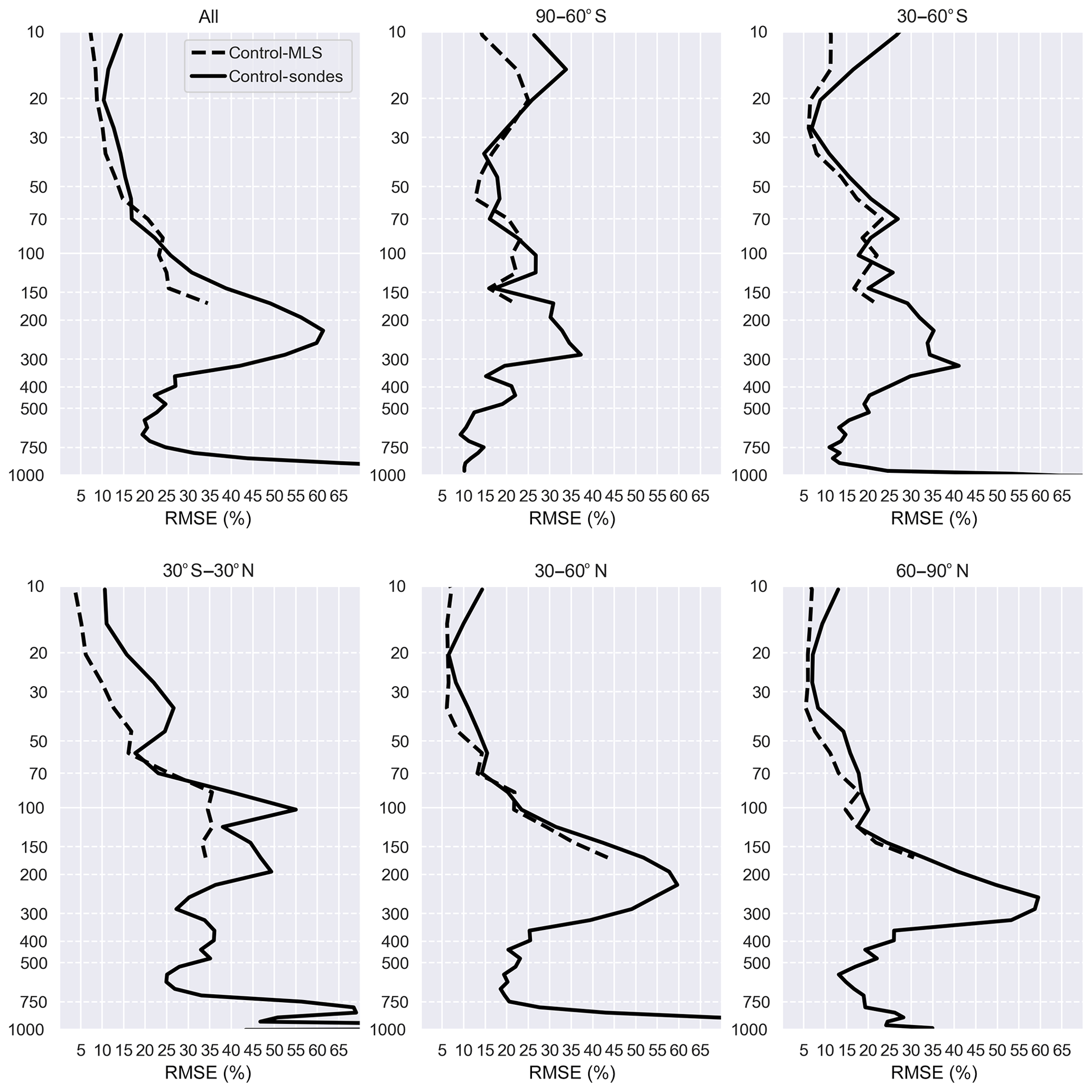
Figure 3Relative root mean square error (RMSE) of the control simulation with respect to radiosoundings (solid lines) and MLS (dotted lines) averaged globally (first plot) and for five separate latitude bands (90–60∘ S, 60–30∘ S, 30∘ S–30∘ N, 30–60∘ N, 60–90∘ N). To compute the percentage, the RMSE statistics have been divided by the corresponding average profile of the observations (radiosoundings or MLS) for each band.
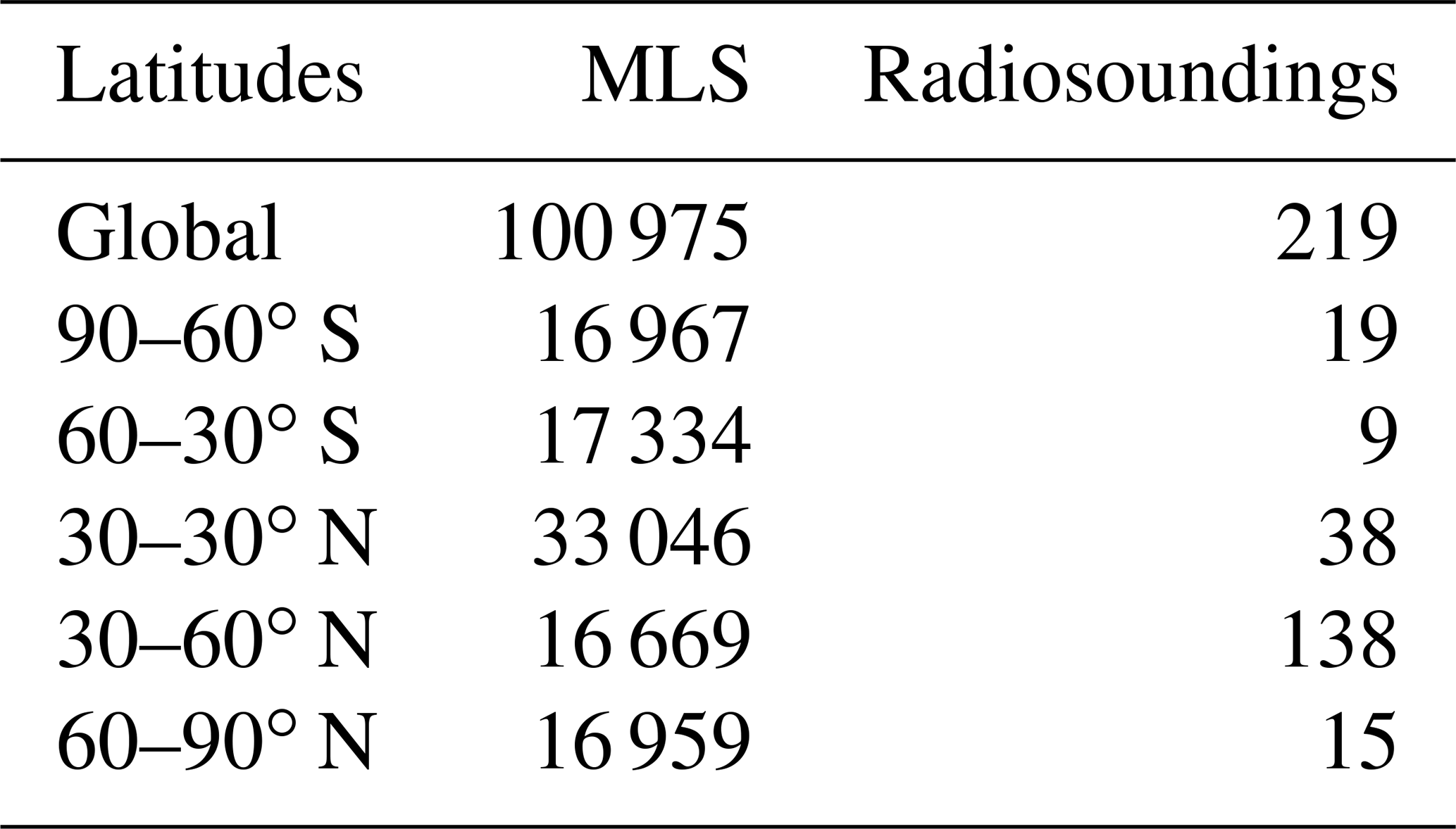
Concerning the standard deviation, Emili et al. (2014) and Peiro et al. (2018) employed vertically varying errors expressed as percentages of the background O3 profile, with larger relative errors in the troposphere and smaller in the stratosphere. Since we use a more detailed chemistry model here (Sect. 3.1), we evaluated the root mean square error (RMSE) of the free model simulation (control) against ozonesondes and MLS profiles (Fig. 3). We remark that the model's RMSE reproduces the vertical features observed in previous studies, with smaller errors in the stratosphere (between 20 and 50 hPa), larger errors in the free troposphere and highest errors close to the tropopause and within the planetary boundary layer. Note also the zonal variability of the maxima, which appear to be linked to the variability of the tropopause height. Thanks to the detailed chemical mechanism, biases (Fig. 4) are generally smaller than in the studies cited previously but remain significant compared to standard deviation values (Fig. 5), especially around the tropopause. Interestingly, RMSE and standard deviation values computed against MLS are generally smaller than those evaluated against ozonesondes, whereas biases are more consistent between the two datasets. We attribute this effect to the larger number of MLS observations (Table 1), which provides more robust standard deviation statistics.

Figure 4Relative bias of the control simulation with respect to radiosoundings (solid lines) and MLS (dotted lines). Same plots as in Fig 3.
The background standard deviation is prescribed through a smooth step function that takes values of 2 % above 50 hPa and 10 % below to reproduce roughly the patterns observed in Fig. 5. Values are smaller than those in Fig. 5 to account for the error reduction during the assimilation, which is particularly strong when MLS observations are used (see Sect. 4.3). Also, neglecting error correlations between IASI channels within R leads to a strong weight towards the observations: reducing the background standard deviation compensates in part for this effect. All the choices made to define B are a result of a large number of assimilation evaluations, in which different options were considered. For example, setting values of 5 % and 25 % leads to less accurate results for both L1 and L2 assimilation (not reported). The percent profile is multiplied by the hourly O3 field of the control simulation once for the entire period and not at every forecast time step. Therefore, all assimilation experiments presented in this study are based on the same B matrix. This choice was made to permit a stricter comparison between L1 and L2 assimilation experiments.

Figure 5Relative standard deviation of the control simulation with respect to radiosoundings (solid lines) and MLS (dotted lines). Same plots as in Fig. 3.
The vertical error correlation diffuses the assimilation increments between model levels and has been found to significantly impact the quality of O3 analyses with current model vertical resolutions (not shown). In general, small values of vertical correlation are favoured in the stratosphere due to the stratification and to avoid injection of large stratospheric O3 increments in the troposphere, whereas larger values are expected within the troposphere due to vertical mixing. In this study a constant value of one model level defines the length scale of the Gaussian correlation (Sect. 3.3). Different choices for the stratosphere and troposphere did not lead to particular improvements (not shown).
Finally, the exponential scale of the horizontal error correlation is set to be equal to 200 km, with the zonal component that is reduced towards the poles to account for the increasing resolution of the model's grid (Emili et al., 2014).
The choice of the background and observation errors is relatively simplistic in this study. Further improvements of the B parameterization could be achieved by diagnosing the forecast errors hourly (Desroziers et al., 2005) or using ensembles of model forecasts. However, more complex and costly estimations do not always improve the results of chemical assimilation systematically and significantly (Massart et al., 2012). Moreover, a good estimation of B cannot be done independently of that of R, which is kept fixed here on purpose. Additional research is needed in this regard, which is beyond the scope of this study.
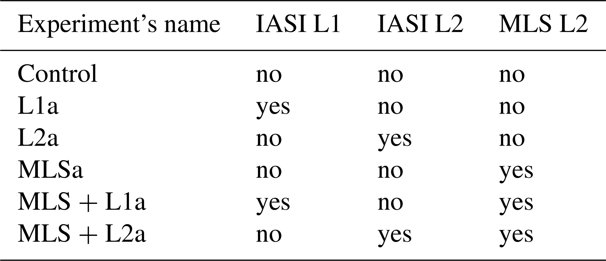
A total of six simulations for the month of July 2010 have been performed (Table 3), starting on 1 July: a free model simulation (control) and five 3D-Var analyses assimilating SOFRID L2 profiles (named L2a), IASI L1 radiances (L1a), MLS L2 profiles (MLSa), MLS plus SOFRID L2 profiles (MLS + L2a) and MLS plus L1 radiances (MLS + L1a). The first three simulations (control, L2a and L1a) are discussed in Sect. 4.1. The control simulation and the three analyses that include MLS are discussed in Sect. 4.3. All simulations have been validated against ozonesondes profiles to elucidate the differences of the resulting O3 vertical distribution. A total of 219 radiosoundings are available globally for July 2010 (Table 1). The co-location of ozonesonde profiles with model fields in time and space is performed through the MOCAGE observation operator (Sect. 3).
4.1 IASI assimilation
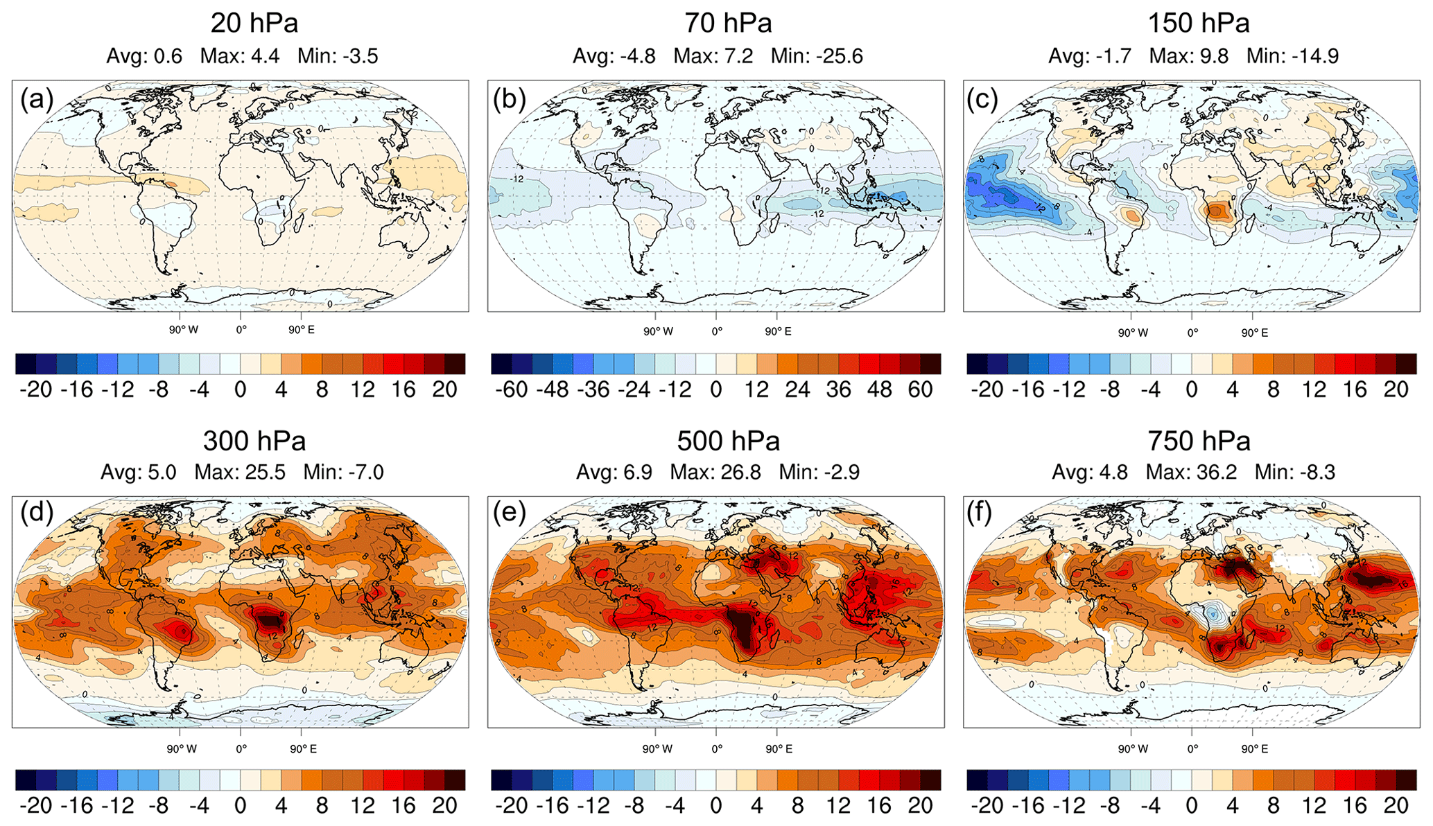
The average O3 values of the control simulation are displayed in Fig. 6. O3 fields have been first interpolated vertically from the model grid to a selection of pressure levels, covering both the stratosphere and the troposphere, and averaged afterwards. The maps show well known properties of the O3 distribution such as the strong zonal gradients in the stratosphere and the presence of local minima in the tropical free troposphere due to deep convection. The average difference between the control simulation and the fixed a priori profile used in SOFRID retrievals (Sect. 2.1.2) is displayed in Fig. 7. Large differences (>100 %) are found at low latitudes both in the lower stratosphere and in the troposphere, with largest values close to the tropical tropopause (150 hPa). This is expected since the SOFRID a priori profile is based on a global ozonesonde climatology that is more representative of mid-latitude O3 profiles (Sect. 2.1.2).
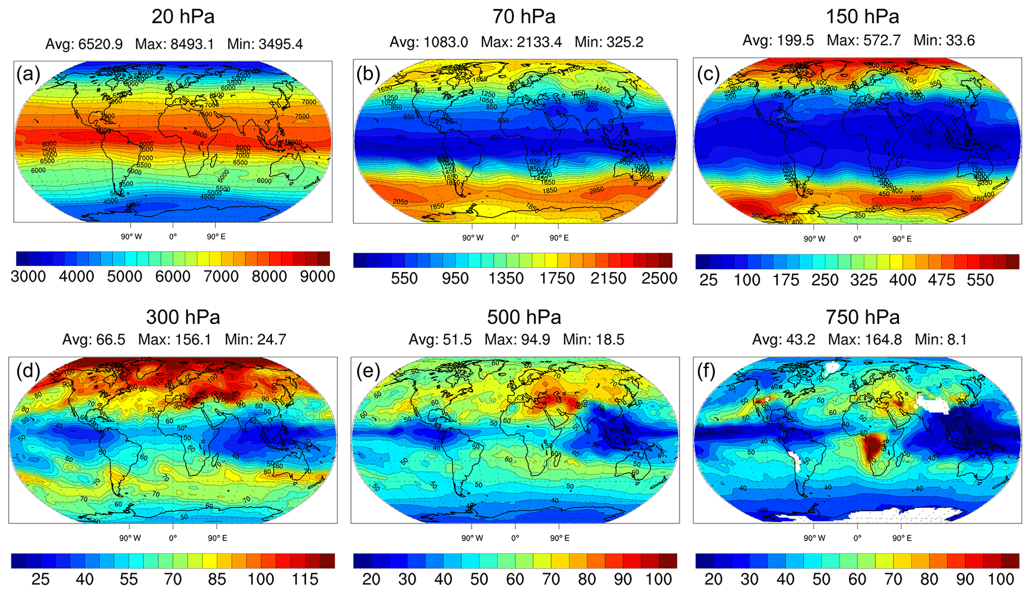
Figure 6Average O3 values of the control simulation in units of parts per billion (ppb) for July 2010. From left to right, different pressure levels are displayed covering the stratosphere (a, b, c) and the free troposphere (d, e, f). Average, maximum and minimum values of the displayed fields are given above each map.
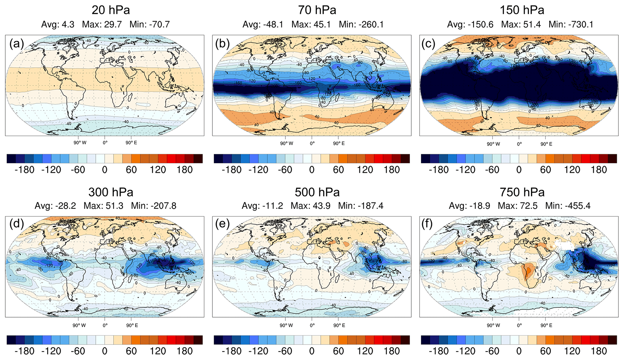
We discuss the geographical differences between L1a and L2a analyses by looking at the monthly bias between the two experiments, divided by the average O3 of the control simulation (Fig. 6). Relative differences are displayed in Fig. 8. First, we remark that differences are generally significant both in the stratosphere and in the troposphere, with absolute values that can exceed 50 % of the O3 field locally and global averages as high as to 20 %. Largest differences in the stratosphere are found at tropical latitudes, L1a showing larger O3 values than L2a at 20 hPa and lower at 70 hPa. In the troposphere the strongest positive differences are still found in the tropics, especially over central Africa, eastern Asia, South America and Middle East regions. Differences become smaller when moving down to 750 hPa and tend to disappear at lower altitudes (not shown), which is normal considering the vertical sensitivity of IASI. At mid-latitudes and high latitudes, relative differences are smaller than at the tropics. This behaviour is consistent with the fact that the SOFRID prior information is much less accurate for tropical latitudes than for mid-latitudes and high latitudes (Fig. 7). Overall, these plots suggest that when the L2 a priori profile is strongly biased (>100 %), the equivalence between L1 and L2 assimilation in the thermal infrared is not verified for O3, even when the averaging kernels are employed.
To confirm that the observed differences are not a consequence of the slightly different NWP inputs used in L1 assimilation and L2 retrievals (Table 2) we rerun the L1a simulation using exactly the same SST a priori values used in SOFRID retrievals. Since we cannot use the same water vapour and temperature profiles of SOFRID within L1a due to the different vertical grids, a different approach has been used: we repeated all assimilation experiments but using ERA Interim (Dee et al., 2011) instead of the NWP forecasts as meteorological forcing for the CTM. This increases potential differences between the L1 and L2 assimilation, due to the different configurations of operational NWP and ERA Interim (model resolution, assimilated instruments, etc.). In all the above cases we obtained very similar results to those presented in Fig. 8 (not shown), which suggests that differences between L1a and L2a discussed previously do not depend on the auxiliary RTM inputs.
To further verify which one out of the L1a and L2a experiments reproduces the measured O3 profiles better, we validated the three simulations against radiosoundings. Figure 9 reports the RMSE differences computed globally and for five different latitude bands. The displayed values are the differences between the RMSE of the assimilation experiment and the corresponding value for the control simulation (Fig. 3). Negative values in Fig. 9 indicate that the assimilation improved the O3 field and decreased the relative RMSE with respect to ozonesondes by the amount displayed on the plot. Looking at the global averages we remark that below 70 hPa the gain is similar for both L1a and L2a experiments and quite significant at 200 hPa (20 %). Note, however, the strong similarity between the global and 30–60∘ N statistics, due to the over-representation of ozonesondes for the Northern Hemisphere (NH) mid-latitudes (63 % of the total).
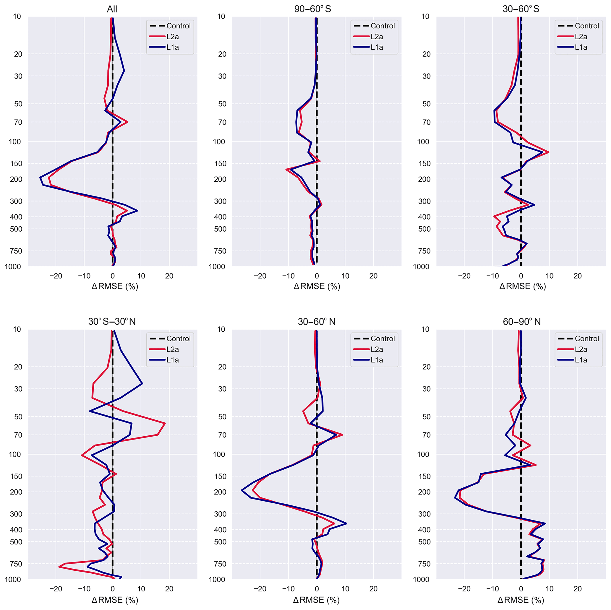
Figure 9Relative difference of RMSE (ΔRMSE) with respect to radiosoundings for L1a (blue) and L2a (red). The difference is computed by subtracting the RMSE of L1a (L2a) from the RMSE of the control simulation (Fig. 3). Negative values mean that the assimilation improved (decreased) the RMSE of the control simulation, and positive values indicate degradation (increase) of the RMSE. The statistics are computed for the same latitudes as in Fig. 3.
In the NH the RMSE of the control simulation is effectively reduced between 70 and 300 hPa (up to 20 %). L1a shows a slightly better gain than L2a between 150 and 300 hPa. Interestingly, both L1a and L2a display increased RMSE between 300 and 400 hPa. This behaviour is also confirmed when the vertical error correlation is switched off in the 3D-Var B and with different choices for the vertical interpolation of O3 optical coefficients within RTTOV (log-linear or Rochon, not shown). Since large negative biases were present in the control simulation (as low as −30 %; see Fig. 4), a possible explanation is that part of the strong positive correction of O3 between 100 and 300 hPa is propagated downwards, where both absolute O3 concentrations and relative biases are much lower. This can degrade the analysis accuracy below 300 hPa. Whether this propagation is carried out by the Jacobian matrix of the observation operator (either through the RTM or the retrieval's AK) or by vertical O3 transport is not yet elucidated and would need further investigation. Also, other possible factors affecting the accuracy of the RTM exist, like inadequate vertical resolution close to the tropopause or uncertainties in meteorological profiles or in the impact of aerosols. Nonetheless, these errors impact both L1a and L2a in our study: further optimization of the L1 assimilation configuration with respect to the L2 retrievals is left for a future study. The RMSE is reduced again at about 500 hPa between 30 and 60∘ N, although not very significantly. The assimilation increases the RMSE of the tropospheric profile (350–1000 hPa) at northern latitudes (60–90∘ N). In general, the validation confirms that L1a and L2a have a very similar accuracy in NH at mid-latitudes and high latitudes, as also suggested previously by Fig. 8. However, the strongest positive corrections are confined to the UTLS.
At the tropics (30∘ S–30∘ N) the results differ more significantly. In the troposphere (below 100 hPa), both L1a and L2a reduced the RMSE of the control simulation, although by a smaller amount than in the NH (5 %). Note also that L1a RMSE reduction is larger than L2a between 400 and 600 hPa, whereas it is the other way around at about 250 and 800 hPa. Above 100 hPa we observe an increase of RMSE that peaks at 60 hPa with L2a and at 30 hPa with L1a but smaller in magnitude for L1a. This behaviour might be linked to the strong differences that exist between the SOFRID prior information and the modelled O3 at the tropical tropopause, to some other factor affecting the RT computations, to overestimation of the background error covariances or to a complex combination of all previous causes. A full satisfactory explanation has not been found yet.
Results in the Southern Hemisphere (SH) (30–90∘ S) are again similar: a lower RMSE than for the control simulation is found for both L1a and L2a in the upper and lower stratosphere (between 30 and 100 hPa and between 150 and 300 hPa). An improvement is also found in the troposphere (400–600 hPa) at mid-latitudes (30–60∘ S), but the low number of ozonesondes available in this band (Table 1) requires a more careful interpretation.

Figure 10Relative difference of RMSE (ΔRMSE) with respect to MLS profiles for L1a (blue) and L2a (red). Same plots as in Fig. 9.
Since radiosoundings do not provide a uniform global coverage, and vertical coverage is also lacking in the vicinity of the O3 maximum, we validated the three simulations against MLS measurements. The RMSE differences for stratospheric profiles can be found in Fig. 10. These statistics are based on more than 105 profiles for the global average and between 15 000 and 30 000 for zonal averages, depending on the latitude band (Table 1). The patterns observed in the stratosphere with respect to ozonesondes are also confirmed with MLS. The only exceptions are a smaller RMSE degradation at 50 hPa for L2a in the tropics and for both L1a and L2a at 150 hPa in the 30–60∘ S band. Higher confidence should be given to the RMSE values provided by MLS than those obtained with radiosoundings (see also Fig. 3 and the relative discussion in Sect. 3.4). However, a similar RMSE behaviour is observed overall, and this bolsters the robustness of the conclusions derived with the radiosoundings in the troposphere.
4.2 Computational cost
The computational cost of L1 assimilation is necessarily higher than for L2 assimilation. Additional CPU time is due not only to online RTM computations but also to a higher number of iterations needed by the minimizer to converge. For a typical 24 h long simulation performed on Intel Xeon E5-2680 V3 CPU, the total CPU time is 3.9 CPU hours for L2a and 13.2 CPU hours for L1a. Note that the L2a time does not include the cost of the L1 to L2 processor but only the cost of the 3D-Var assimilation plus the model forecasts. Most of the CPU time for L1a is spent on the linearized and adjoint calls of the RTM (50 % of the total CPU time), whereas the corresponding time spent for the observation operator within the L2a experiment is about 1 %. However, the total CPU time can be significantly decreased by reducing the maximum number of iterations of the minimizer. A simulation with a halved number of iterations (75) showed very similar results to the ones that have been reported (150 iterations) and could be considered if computation time is a critical factor. Moreover, with standard high-performance computers, and thanks to the parallel nature of the observation operator and the RTM, we could obtain a speed-up of about 24 on the 24 CPU cores. This reduces the runtime of L1a to about 36 min for the 24 h long simulation versus 13 min for L2a. The extra cost of L1 assimilation therefore also seems acceptable for operational applications.
4.3 IASI and MLS assimilation
Some issues were identified in the previous section in the stratosphere, especially at tropical latitudes. Among possible reasons, one is that inversion of TIR measurements might be particularly sensitive to the vertical distribution of O3 in the tropical stratosphere. We consider assimilating MLS L2 profiles in combination with IASI here to correct the model stratosphere and troposphere simultaneously, as also done in previous studies (Emili et al., 2014; Peiro et al., 2018). When the radiances are assimilated, the RT problem is solved for the entire atmospheric column within the iterations of the variational algorithm. Therefore, enhanced and better synergies could be observed than when only L2 products are assimilated.
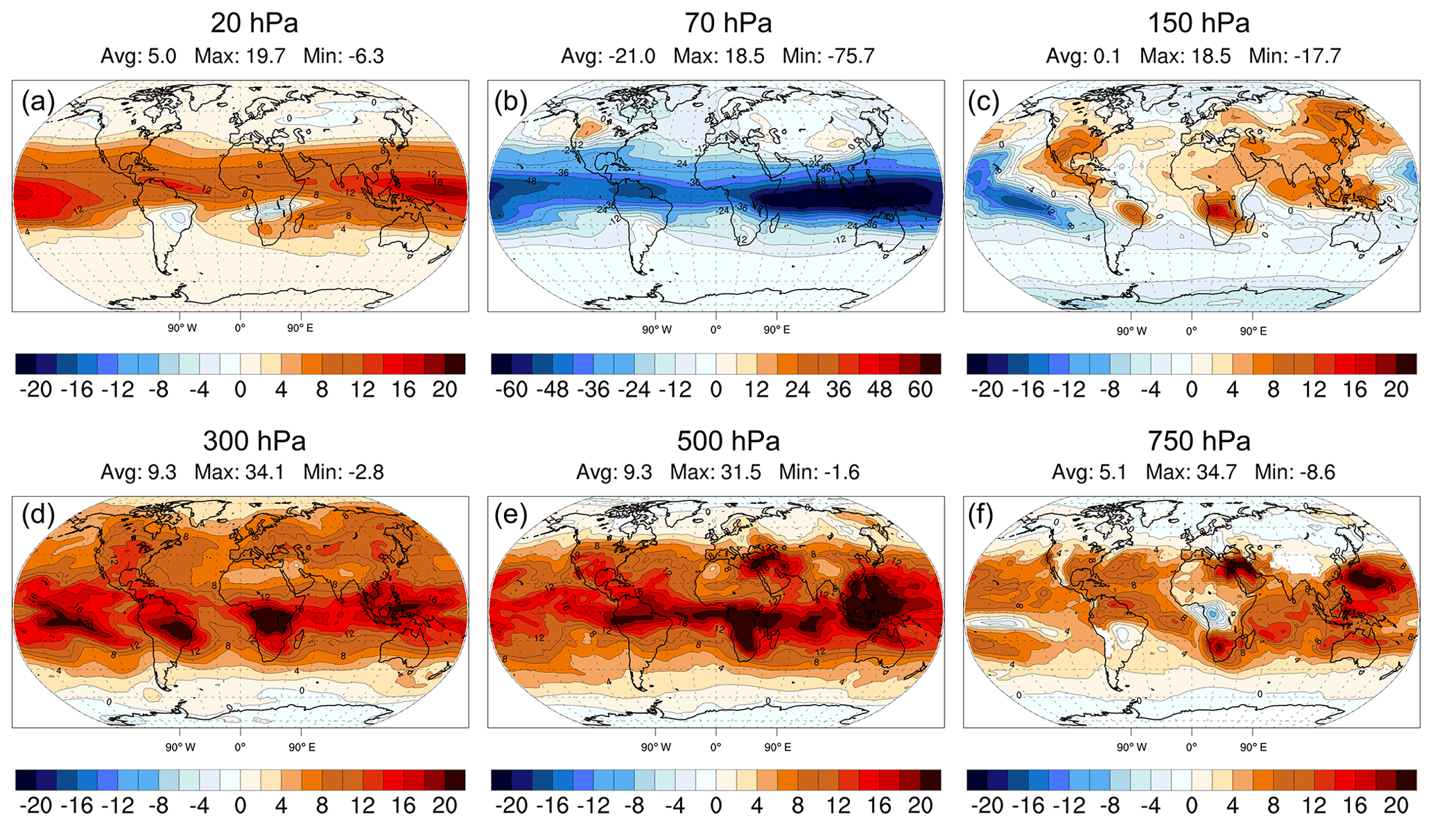
We report in Fig. 11 the impact of assimilating MLS in combination with IASI L1 and L2 by computing the average differences between MLS + L1a and MLS + L2a. We remark that the differences in the stratosphere are highly reduced with respect to Fig. 8, which is expected due to the direct constraint of MLS observations. Significant differences (>10 %) remain below 150 hPa, with patterns and sign similar to those in Fig. 8. The amplitude of the differences is, however, also slightly reduced at 300 and 500 hPa.
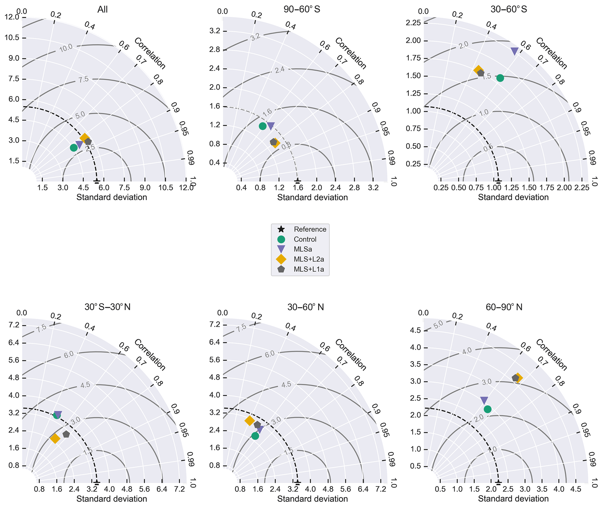
Figure 13Taylor diagrams of modelled tropospheric ozone columns (340–750 hPa) for the Control simulation (green), MLSa (violet), MLS + L1a (grey) and MLS + L2a (yellow) averaged globally and for five separate latitude bands. The Taylor statistics are computed against radiosoundings.
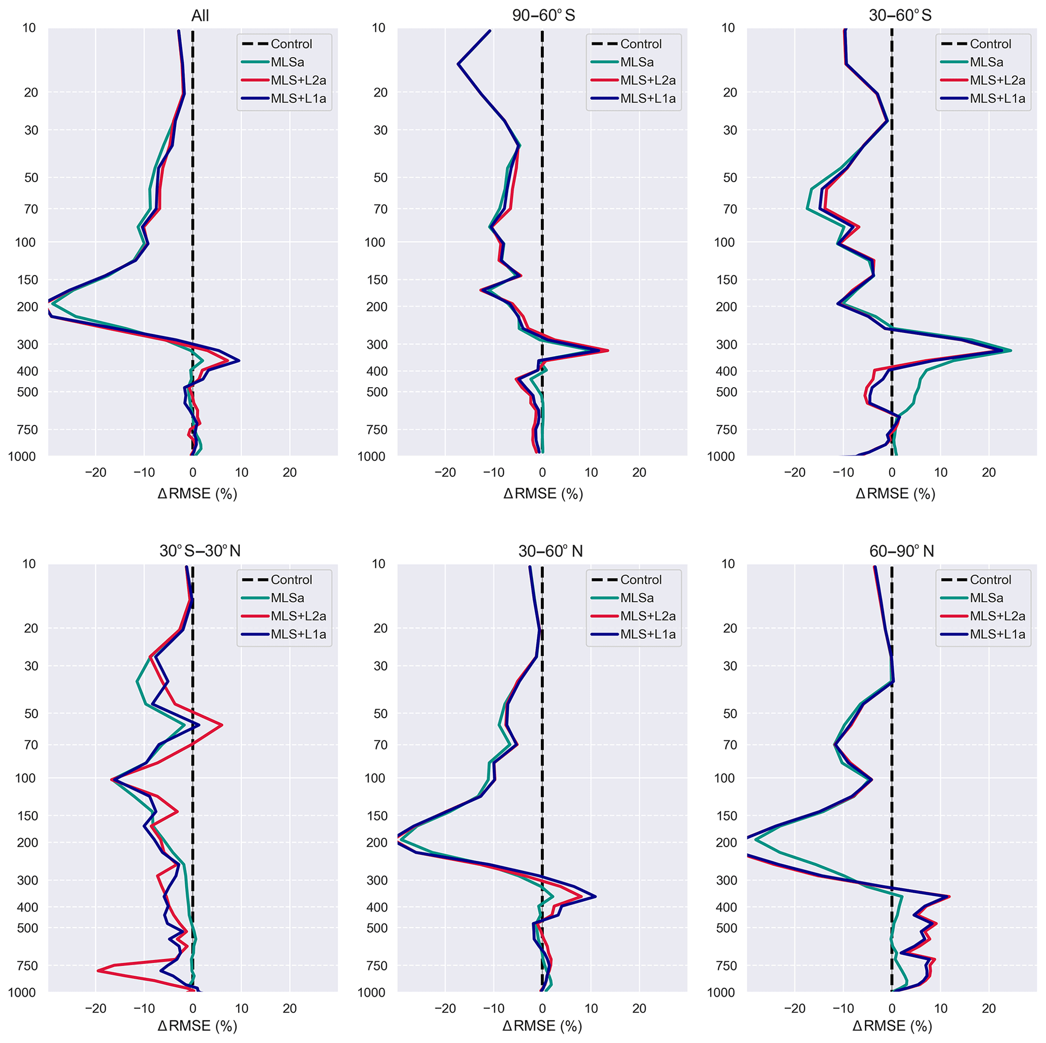
We compared the RMSE of MLSa, MLS + L1a and MLS + L2a computed against ozonesondes (Fig. 12) to evaluate if the joint assimilation improves the overall O3 distribution. MLSa provides particularly accurate results down to 200 or 300 hPa, depending on the latitude, with a robust reduction of the RMSE with respect to the control simulation. The only exception is in the SH mid-latitudes below 250 hPa, where the MLSa RMSE increases. We suspect that this might be linked again to the combination of strong O3 gradients at the tropopause height and the negative bias of the control simulation above the tropopause (see Sect. 4.1). Overall MLSa confirms results found in past studies (Massart et al., 2012; Emili et al., 2014) and represents much better prior information for assimilation of radiances or retrievals.
We remark that MLS + L1a and MLS + L2a now provide closer results in the NH and in the tropics compared to Fig. 9. The stratospheric O3 gain is much more significant with MLS + L1a and MLS + L2a than with L1a and L2a and remains very close to MLSa, demonstrating that assimilating accurate stratospheric profiles remains essential for O3 reanalyses. The only region where IASI further improves the UTLS profile with respect to MLSa is in the NH: a positive, albeit small, effect of assimilating IASI in combination with MLS is found between 150 and 300 hPa. On the other hand, below 300 hPa, the addition of MLS (Fig. 12) does not bring further improvements with respect to IASI alone (Fig. 9). We can conclude that MLS corrects most of the errors introduced by IASI assimilation in the stratosphere (Fig. 9), but no particular synergy is observed in the case of MLS and L1 assimilation in the troposphere.
In Fig. 13 we report the Taylor plots concerning the free troposphere O3 column (340–750 hPa), to further evaluate the skills of the assimilation experiments in terms of variability. We examine the free troposphere here since it is where the direct impact of IASI assimilation is the largest and the impact of MLS the smallest (except for the 30–60∘ S band). IASI assimilation improves the variability of the modelled O3 field when looking at global averages, but this conclusion varies as a function of the latitude band. Robust and significant improvements are only found at the tropics and in the SH polar region; mixed results are obtained elsewhere. This confirms previous findings obtained with L2 assimilation (Emili et al., 2014) and adds the conclusion that better prior information does not necessarily solve all issues related to the assimilation of TIR measurements at mid-latitudes and high latitudes. Nevertheless, the assimilation of radiances provides slightly better results at all latitudes in general and permits more variability to be extracted from IASI spectra, especially at tropical latitudes.
In this study we addressed the following question: what are the differences between the direct assimilation of IASI radiances (Level 1) and the assimilation of Level 2 products for O3 analyses and reanalyses? We used an experimental setup in which differences between the L2 retrieval and the L1 assimilation have been minimized as much as possible, for example by using the same RTM (RTTOV) and control vector (O3 and SST) in both approaches. This allowed the impact of the O3 prior information and its error covariance on the quality of the analysis to be delved into.
We performed twin assimilation experiments with the MOCAGE CTM and the SOFRID O3 retrievals, using the same IASI ground pixels for both L1 and L2 assimilation, named L1a and L2a respectively. We compared the obtained analyses against each other and against ozonesondes and MLS profiles for the month of July 2010.
The results suggest that the accuracy of the O3 prior information used in the L2 retrievals can influence the analysis, even when the averaging kernels are employed within the assimilation. When the O3 prior information is strongly biased (at low latitudes in this study), L1a and L2a differ significantly (>10 %) and the analysis shows a better variability when assimilating directly L1 radiances instead of L2 profiles. L1a and L2a are otherwise very similar at mid-latitudes and high latitudes, where the SOFRID prior information is closer to the true O3 profile.
We conclude that particular care should be taken before assimilating satellite retrievals with prior information that can, in some circumstances, differ significantly from the local ozone profile. Computing retrievals using an a priori profile issued from a model could be relevant in improving current IASI O3 L2 products and might reduce the differences between L2a and L1a observed in our study. Preliminary results with SOFRID based on a modelled a priori profile also show significant differences with the original product (Brice Barret, personal communication, 2019), with patterns similar to those presented in this study. However, when the final purpose is data assimilation, the L1 approach is more practical and statistically consistent, especially in the case that the observations need to be assimilated within the same forecast model that was used to compute L2 retrievals.
A positive impact has been found when assimilating MLS profiles and IASI simultaneously (either L1 or L2), which corrected stratospheric biases due to IASI assimilation alone. Differences between L1 and L2 assimilation are globally reduced by MLS in the stratosphere but remain significant (>10 %) in the tropical troposphere. Also, MLS assimilation strongly improves the model's accuracy down to 200 hPa, and a clear added value of IASI assimilation (L1 or L2) can only be observed in the tropical troposphere. These results remind us that the information brought by limb sounders like MLS into the DA system remains essential to improve upper stratosphere O3. Interesting perspectives for future work are to (i) verify whether the assimilation of O3 retrievals from UV spectrometers like GOME-2 or TROPOMI also shows issues related to the a priori dependence and (ii) examine if UV assimilation could replace MLS when assimilated jointly with IASI and provide similar performances in the stratosphere. This will be important to ensure the capacity to carry out accurate O3 reanalyses when the MLS instrument is phased out.
We reckon that L1 assimilation requires the full atmosphere to be modelled, which may not be available to some models, for example those conceived exclusively for tropospheric applications. Moreover, Level 2 products can be aggregated vertically to correct some model layers selectively and averaged spatially to fit models with coarser resolution than the satellite ground-pixel size. This cannot easily be done with radiances and should be addressed in future research.
In this study the observations, their error covariance and the RTM auxiliary inputs were kept almost identical between L1 and L2 assimilation on purpose. Further research is needed to address issues that are common to L1 and L2 assimilation, e.g. increased errors close to the tropopause in the NH or in the tropical stratosphere. Improvements are expected, for example, by increasing the vertical resolution of the model, including modelled aerosols within the RT or using more realistic observation error covariances. Including more modelled variables among the RTM inputs is in particular of interest in the context of the evolution towards ESMs, for which hyper-spectral sounders like IASI can provide very valuable constraints for multi-variate reanalyses (atmosphere plus surface). Including inter-channel and ground-pixel correlations in the observation error covariance matrix seems necessary to correctly weight very dense IASI observations within higher-resolution models than the one used in this study. All these aspects deserve further research.
The input data used in this study are freely accessible through the web pages reported in the paper, if not stated differently. Access to operational ECMWF (https://www.ecmwf.int/en/forecasts/accessing-forecasts, last access: 18 July 2019) analyses and forecasts used to run the chemical transport model is subject to some particular conditions. All results are available upon request to the author.
EE performed the numerical experiments and wrote the manuscript. BB and EF computed SOFRID retrievals used as input for some of the experiments. DC helped with the setup of the chemistry transport model.
The authors declare that they have no conflict of interest.
We acknowledge EUMETSAT for providing IASI L1C data, WOUDC for providing ozonesondes data and the NASA Jet Propulsion Laboratory for the availability of Aura MLS Level 2 O3. We also thanks the MOCAGE team at Météo-France for providing the chemical transport model, the RTTOV team for the radiative transfer model and Andrea Piacentini and Gabriel Jonville for their help with technical developments of the assimilation code. This work was possible thanks to the financial support from the Région Midi-Pyrénées, who sponsored the preliminary work of Hélène Peiro on the subject, and CNES (Centre National d'Études Spatiales), through the TOSCA program.
This paper was edited by Mark Weber and reviewed by two anonymous referees.
Andersson, E., Pailleux, J., Thépaut, J.-N., Eyre, J. R., McNally, A. P., Kelly, G. A., and Courtier, P.: Use of cloud-cleared radiances in three/four-dimensional variational data assimilation, Q. J. Roy. Meteor. Soc., 120, 627–653, https://doi.org/10.1002/qj.49712051707, 1994. a
Barré, J., Peuch, V.-H., Lahoz, W. A., Attié, J.-L., Josse, B., Piacentini, A., Eremenko, M., Dufour, G., Nedelec, P., von Clarmann, T., and El Amraoui, L.: Combined data assimilation of ozone tropospheric columns and stratospheric profiles in a high-resolution CTM, Q. J. Roy. Meteor. Soc., 140, 966–981, https://doi.org/10.1002/qj.2176, 2013. a
Barret, B., Le Flochmoen, E., Sauvage, B., Pavelin, E., Matricardi, M., and Cammas, J. P.: The detection of post-monsoon tropospheric ozone variability over south Asia using IASI data, Atmos. Chem. Phys., 11, 9533–9548, https://doi.org/10.5194/acp-11-9533-2011, 2011. a, b, c, d, e, f, g
Bocquet, M., Elbern, H., Eskes, H., Hirtl, M., vZabkar, R., Carmichael, G. R., Flemming, J., Inness, A., Pagowski, M., Pérez Camaño, J. L., Saide, P. E., San Jose, R., Sofiev, M., Vira, J., Baklanov, A., Carnevale, C., Grell, G., and Seigneur, C.: Data assimilation in atmospheric chemistry models: current status and future prospects for coupled chemistry meteorology models, Atmos. Chem. Phys., 15, 5325–5358, https://doi.org/10.5194/acp-15-5325-2015, 2015. a
Borbas, E. E. and Ruston, B. C.: The RTTOV UWiremis IR land surface emissivity module, Tech. rep., NP-SAF report, available at: http://nwpsaf.eu/vs_reports/nwpsaf-mo-vs-042.pdf (last access: 16 July 2019), 2010. a, b, c
Boynard, A., Hurtmans, D., Koukouli, M. E., Goutail, F., Bureau, J., Safieddine, S., Lerot, C., Hadji-Lazaro, J., Wespes, C., Pommereau, J.-P., Pazmino, A., Zyrichidou, I., Balis, D., Barbe, A., Mikhailenko, S. N., Loyola, D., Valks, P., Van Roozendael, M., Coheur, P.-F., and Clerbaux, C.: Seven years of IASI ozone retrievals from FORLI: validation with independent total column and vertical profile measurements, Atmos. Meas. Tech., 9, 4327–4353, https://doi.org/10.5194/amt-9-4327-2016, 2016. a, b
Brown, A., Milton, S., Cullen, M., Golding, B., Mitchell, J., and Shelly, A.: Unified Modeling and Prediction of Weather and Climate: A 25-Year Journey, B. Am. Meteorol. Soc., 93, 1865–1877, https://doi.org/10.1175/BAMS-D-12-00018.1, 2012. a
Clerbaux, C., Boynard, A., Clarisse, L., George, M., Hadji-Lazaro, J., Herbin, H., Hurtmans, D., Pommier, M., Razavi, A., Turquety, S., Wespes, C., and Coheur, P.-F.: Monitoring of atmospheric composition using the thermal infrared IASI/MetOp sounder, Atmos. Chem. Phys., 9, 6041–6054, https://doi.org/10.5194/acp-9-6041-2009, 2009. a, b
Coman, A., Foret, G., Beekmann, M., Eremenko, M., Dufour, G., Gaubert, B., Ung, A., Schmechtig, C., Flaud, J.-M., and Bergametti, G.: Assimilation of IASI partial tropospheric columns with an Ensemble Kalman Filter over Europe, Atmos. Chem. Phys., 12, 2513–2532, https://doi.org/10.5194/acp-12-2513-2012, 2012. a
Dee, D. P. and Uppala, S.: Variational bias correction of satellite radiance data in the ERA-Interim reanalysis, Q. J. Roy. Meteor. Soc., 135, 1830–1841, https://doi.org/10.1002/qj.493, 2009. a
Dee, D. P., Uppala, S. M., Simmons, A. J., Berrisford, P., Poli, P., Kobayashi, S., Andrae, U., Balmaseda, M. A., Balsamo, G., Bauer, P., Bechtold, P., Beljaars, A. C. M., van de Berg, L., Bidlot, J., Bormann, N., Delsol, C., Dragani, R., Fuentes, M., Geer, A. J., Haimberger, L., Healy, S. B., Hersbach, H., Hólm, E. V., Isaksen, L., Kållberg, P., Köhler, M., Matricardi, M., McNally, A. P., Monge-Sanz, B. M., Morcrette, J.-J., Park, B.-K., Peubey, C., de Rosnay, P., Tavolato, C., Thépaut, J.-N., and Vitart, F.: The ERA-Interim reanalysis: configuration and performance of the data assimilation system, Q. J. Roy. Meteor. Soc., 137, 553–597, https://doi.org/10.1002/qj.828, 2011. a
Desroziers, G., Berre, L., Chapnik, B., and Poli, P.: Diagnosis of observation, background and analysis-error statistics in observation space, Q. J. Roy. Meteor. Soc., 131, 3385–3396, https://doi.org/10.1256/qj.05.108, 2005. a
De Wachter, E., Barret, B., Le Flochmoën, E., Pavelin, E., Matricardi, M., Clerbaux, C., Hadji-Lazaro, J., George, M., Hurtmans, D., Coheur, P.-F., Nedelec, P., and Cammas, J. P.: Retrieval of MetOp-A/IASI CO profiles and validation with MOZAIC data, Atmos. Meas. Tech., 5, 2843–2857, https://doi.org/10.5194/amt-5-2843-2012, 2012. a
Dufour, G., Eremenko, M., Griesfeller, A., Barret, B., LeFlochmoën, E., Clerbaux, C., Hadji-Lazaro, J., Coheur, P.-F., and Hurtmans, D.: Validation of three different scientific ozone products retrieved from IASI spectra using ozonesondes, Atmos. Meas. Tech., 5, 611–630, https://doi.org/10.5194/amt-5-611-2012, 2012. a, b, c, d
Emili, E., Barret, B., Massart, S., Le Flochmoen, E., Piacentini, A., El Amraoui, L., Pannekoucke, O., and Cariolle, D.: Combined assimilation of IASI and MLS observations to constrain tropospheric and stratospheric ozone in a global chemical transport model, Atmos. Chem. Phys., 14, 177–198, https://doi.org/10.5194/acp-14-177-2014, 2014. a, b, c, d, e, f, g, h, i, j, k, l, m
Eskes, H. J. and Boersma, K. F.: Averaging kernels for DOAS total-column satellite retrievals, Atmos. Chem. Phys., 3, 1285–1291, https://doi.org/10.5194/acp-3-1285-2003, 2003. a
Eyre, J. R., Kelly, G. A., McNally, A. P., Andersson, E., and Persson, A.: Assimilation of TOVS radiance information through one-dimensional variational analysis, Q. J. Roy. Meteor. Soc., 119, 1427–1463, https://doi.org/10.1002/qj.49711951411, 1993. a
Flemming, J., Huijnen, V., Arteta, J., Bechtold, P., Beljaars, A., Blechschmidt, A.-M., Diamantakis, M., Engelen, R. J., Gaudel, A., Inness, A., Jones, L., Josse, B., Katragkou, E., Marecal, V., Peuch, V.-H., Richter, A., Schultz, M. G., Stein, O., and Tsikerdekis, A.: Tropospheric chemistry in the Integrated Forecasting System of ECMWF, Geosci. Model Dev., 8, 975–1003, https://doi.org/10.5194/gmd-8-975-2015, 2015. a
Flemming, J., Benedetti, A., Inness, A., Engelen, R. J., Jones, L., Huijnen, V., Remy, S., Parrington, M., Suttie, M., Bozzo, A., Peuch, V.-H., Akritidis, D., and Katragkou, E.: The CAMS interim Reanalysis of Carbon Monoxide, Ozone and Aerosol for 2003–2015, Atmos. Chem. Phys., 17, 1945–1983, https://doi.org/10.5194/acp-17-1945-2017, 2017. a, b
Froidevaux, L., Jiang, Y. B., Lambert, A., Livesey, N. J., Read, W. G., Waters, J. W., Browell, E. V., Hair, J. W., Avery, M. A., McGee, T. J., Twigg, L. W., Sumnicht, G. K., Jucks, K. W., Margitan, J. J., Sen, B., Stachnik, R. A., Toon, G. C., Bernath, P. F., Boone, C. D., Walker, K. A., Filipiak, M. J., Harwood, R. S., Fuller, R. A., Manney, G. L., Schwartz, M. J., Daffer, W. H., Drouin, B. J., Cofield, R. E., Cuddy, D. T., Jarnot, R. F., Knosp, B. W., Perun, V. S., Snyder, W. V., Stek, P. C., Thurstans, R. P., and Wagner, P. A.: Validation of Aura Microwave Limb Sounder stratospheric ozone measurements, J. Geophys. Res., 113, D15S20, https://doi.org/10.1029/2007JD008771, 2008. a
Froidevaux, L., Anderson, J., Wang, H.-J., Fuller, R. A., Schwartz, M. J., Santee, M. L., Livesey, N. J., Pumphrey, H. C., Bernath, P. F., Russell III, J. M., and McCormick, M. P.: Global OZone Chemistry And Related trace gas Data records for the Stratosphere (GOZCARDS): methodology and sample results with a focus on HCl, H2O, and O3, Atmos. Chem. Phys., 15, 10471–10507, https://doi.org/10.5194/acp-15-10471-2015, 2015. a
Gaudel, A., Cooper, O. R., Ancellet, G., Barret, B., Boynard, A., Burrows, J. P., Clerbaux, C., Coheur, P. F., Cuesta, J., Cuevas, E., Doniki, S., Dufour, G., Ebojie, F., Foret, G., Garcia, O., Granados Muños, M. J., Hannigan, J. W., Hase, F., Huang, G., Hassler, B., Hurtmans, D., Jaffe, D., Jones, N., Kalabokas, P., Kerridge, B., Kulawik, S. S., Latter, B., Leblanc, T., Le Flochmoën, E., Lin, W., Liu, J., Liu, X., Mahieu, E., McClure-Begley, A., Neu, J. L., Osman, M., Palm, M., Petetin, H., Petropavlovskikh, I., Querel, R., Rahpoe, N., Rozanov, A., Schultz, M. G., Schwab, J., Siddans, R., Smale, D., Steinbacher, M., Tanimoto, H., Tarasick, D. W., Thouret, V., Thompson, A. M., Trickl, T., Weatherhead, E., Wespes, C., Worden, H. M., Vigouroux, C., Xu, X., Zeng, G., and Ziemke, J.: Tropospheric Ozone Assessment Report: Present-day distribution and trends of tropospheric ozone relevant to climate and global atmospheric chemistry model evaluation, Elem .Sci. Anth., 6, 39, https://doi.org/10.1525/elementa.291, 2018. a
Geer, A. J., Lahoz, W. A., Bekki, S., Bormann, N., Errera, Q., Eskes, H. J., Fonteyn, D., Jackson, D. R., Juckes, M. N., Massart, S., Peuch, V.-H., Rharmili, S., and Segers, A.: The ASSET intercomparison of ozone analyses: method and first results, Atmos. Chem. Phys., 6, 5445–5474, https://doi.org/10.5194/acp-6-5445-2006, 2006. a, b
Han, W. and McNally, A. P.: The 4D-Var assimilation of ozone-sensitive infrared radiances measured by IASI, Q. J. Roy. Meteor. Soc., 136, 2025–2037, https://doi.org/10.1002/qj.708, 2010. a
Hilton, F., Armante, R., August, T., Barnet, C., Bouchard, A., Camy-Peyret, C., Capelle, V., Clarisse, L., Clerbaux, C., Coheur, P.-F., Collard, A., Crevoisier, C., Dufour, G., Edwards, D., Faijan, F., Fourrié, N., Gambacorta, A., Goldberg, M., Guidard, V., Hurtmans, D., Illingworth, S., Jacquinet-Husson, N., Kerzenmacher, T., Klaes, D., Lavanant, L., Masiello, G., Matricardi, M., McNally, A., Newman, S., Pavelin, E., Payan, S., Péquignot, E., Peyridieu, S., Phulpin, T., Remedios, J., Schlüssel, P., Serio, C., Strow, L., Stubenrauch, C., Taylor, J., Tobin, D., Wolf, W., and Zhou, D.: Hyperspectral Earth Observation from IASI: Five Years of Accomplishments, B. Am. Meteorol. Soc., 93, 347–370, https://doi.org/10.1175/BAMS-D-11-00027.1, 2012. a
Hubert, D., Lambert, J.-C., Verhoelst, T., Granville, J., Keppens, A., Baray, J.-L., Bourassa, A. E., Cortesi, U., Degenstein, D. A., Froidevaux, L., Godin-Beekmann, S., Hoppel, K. W., Johnson, B. J., Kyrölä, E., Leblanc, T., Lichtenberg, G., Marchand, M., McElroy, C. T., Murtagh, D., Nakane, H., Portafaix, T., Querel, R., Russell III, J. M., Salvador, J., Smit, H. G. J., Stebel, K., Steinbrecht, W., Strawbridge, K. B., Stübi, R., Swart, D. P. J., Taha, G., Tarasick, D. W., Thompson, A. M., Urban, J., van Gijsel, J. A. E., Van Malderen, R., von der Gathen, P., Walker, K. A., Wolfram, E., and Zawodny, J. M.: Ground-based assessment of the bias and long-term stability of 14 limb and occultation ozone profile data records, Atmos. Meas. Tech., 9, 2497–2534, https://doi.org/10.5194/amt-9-2497-2016, 2016. a
Hurrell, J. W., Holland, M. M., Gent, P. R., Ghan, S., Kay, J. E., Kushner, P. J., Lamarque, J.-F., Large, W. G., Lawrence, D., Lindsay, K., Lipscomb, W. H., Long, M. C., Mahowald, N., Marsh, D. R., Neale, R. B., Rasch, P., Vavrus, S., Vertenstein, M., Bader, D., Collins, W. D., Hack, J. J., Kiehl, J., and Marshall, S.: The Community Earth System Model: A Framework for Collaborative Research, B. Am. Meteorol. Soc., 94, 1339–1360, https://doi.org/10.1175/BAMS-D-12-00121.1, 2013. a
Inness, A., Blechschmidt, A.-M., Bouarar, I., Chabrillat, S., Crepulja, M., Engelen, R. J., Eskes, H., Flemming, J., Gaudel, A., Hendrick, F., Huijnen, V., Jones, L., Kapsomenakis, J., Katragkou, E., Keppens, A., Langerock, B., de Mazière, M., Melas, D., Parrington, M., Peuch, V. H., Razinger, M., Richter, A., Schultz, M. G., Suttie, M., Thouret, V., Vrekoussis, M., Wagner, A., and Zerefos, C.: Data assimilation of satellite-retrieved ozone, carbon monoxide and nitrogen dioxide with ECMWF's Composition-IFS, Atmos. Chem. Phys., 15, 5275–5303, https://doi.org/10.5194/acp-15-5275-2015, 2015. a, b
Jaumouillé, E., Massart, S., Piacentini, A., Cariolle, D., and Peuch, V.-H.: Impact of a time-dependent background error covariance matrix on air quality analysis, Geosci. Model Dev., 5, 1075–1090, https://doi.org/10.5194/gmd-5-1075-2012, 2012. a
Josse, B., Simon, P., and Peuch, V.: Radon global simulations with the multiscale chemistry and transport model MOCAGE, Tellus B, 56, 339–356, https://doi.org/10.1111/j.1600-0889.2004.00112.x, 2004. a
Lahoz, W. A., Geer, A. J., Bekki, S., Bormann, N., Ceccherini, S., Elbern, H., Errera, Q., Eskes, H. J., Fonteyn, D., Jackson, D. R., Khattatov, B., Marchand, M., Massart, S., Peuch, V.-H., Rharmili, S., Ridolfi, M., Segers, A., Talagrand, O., Thornton, H. E., Vik, A. F., and von Clarmann, T.: The Assimilation of Envisat data (ASSET) project, Atmos. Chem. Phys., 7, 1773–1796, https://doi.org/10.5194/acp-7-1773-2007, 2007. a, b
Liu, D. C. and Nocedal, J.: On the limited memory BFGS method for large scale optimization, Math. Program., 45, 503–528, https://doi.org/10.1007/BF01589116, 1989. a
Livesey, N.: Earth Observing System ( EOS ) Version 4 Level data quality and description document, Tech. rep., 2018. a
Marécal, V., Peuch, V.-H., Andersson, C., Andersson, S., Arteta, J., Beekmann, M., Benedictow, A., Bergström, R., Bessagnet, B., Cansado, A., Chéroux, F., Colette, A., Coman, A., Curier, R. L., Denier van der Gon, H. A. C., Drouin, A., Elbern, H., Emili, E., Engelen, R. J., Eskes, H. J., Foret, G., Friese, E., Gauss, M., Giannaros, C., Guth, J., Joly, M., Jaumouillé, E., Josse, B., Kadygrov, N., Kaiser, J. W., Krajsek, K., Kuenen, J., Kumar, U., Liora, N., Lopez, E., Malherbe, L., Martinez, I., Melas, D., Meleux, F., Menut, L., Moinat, P., Morales, T., Parmentier, J., Piacentini, A., Plu, M., Poupkou, A., Queguiner, S., Robertson, L., Rouïl, L., Schaap, M., Segers, A., Sofiev, M., Tarasson, L., Thomas, M., Timmermans, R., Valdebenito, Á., van Velthoven, P., van Versendaal, R., Vira, J., and Ung, A.: A regional air quality forecasting system over Europe: the MACC-II daily ensemble production, Geosci. Model Dev., 8, 2777–2813, https://doi.org/10.5194/gmd-8-2777-2015, 2015. a, b
Massart, S., Clerbaux, C., Cariolle, D., Piacentini, A., Turquety, S., and Hadji-Lazaro, J.: First steps towards the assimilation of IASI ozone data into the MOCAGE-PALM system, Atmos. Chem. Phys., 9, 5073–5091, https://doi.org/10.5194/acp-9-5073-2009, 2009. a, b
Massart, S., Pajot, B., Piacentini, A., and Pannekoucke, O.: On the Merits of Using a 3D-FGAT Assimilation Scheme with an Outer Loop for Atmospheric Situations Governed by Transport, Mon. Weather Rev., 138, 4509–4522, https://doi.org/10.1175/2010MWR3237.1, 2010. a
Massart, S., Piacentini, A., and Pannekoucke, O.: Importance of using ensemble estimated background error covariances for the quality of atmospheric ozone analyses, Q. J. Roy. Meteor. Soc., 138, 889–905, https://doi.org/10.1002/qj.971, 2012. a, b, c, d
McPeters, R. D., Labow, G. J., and Logan, J. A.: Ozone climatological profiles for satellite retrieval algorithms, J. Geophys. Res.-Atmos., 112, 1–9, https://doi.org/10.1029/2005JD006823, 2007. a
Migliorini, S.: On the Equivalence between Radiance and Retrieval Assimilation, Mon. Weather Rev., 140, 258–265, https://doi.org/10.1175/MWR-D-10-05047.1, 2012. a, b
Migliorini, S., Piccolo, C., and Rodgers, C. D.: Use of the Information Content in Satellite Measurements for an Efficient Interface to Data Assimilation, Mon. Weather Rev., 136, 2633–2650, https://doi.org/10.1175/2007MWR2236.1, 2008. a
Mirouze, I. and Weaver, A. T.: Representation of correlation functions in variational assimilation using an implicit diffusion operator, Q. J. Roy. Meteor. Soc., 136, 1421–1443, https://doi.org/10.1002/qj.643, 2010. a
Miyazaki, K., Eskes, H. J., Sudo, K., Takigawa, M., van Weele, M., and Boersma, K. F.: Simultaneous assimilation of satellite NO2, O3, CO, and HNO3 data for the analysis of tropospheric chemical composition and emissions, Atmos. Chem. Phys., 12, 9545–9579, https://doi.org/10.5194/acp-12-9545-2012, 2012. a
Mizzi, A. P., Arellano Jr., A. F., Edwards, D. P., Anderson, J. L., and Pfister, G. G.: Assimilating compact phase space retrievals of atmospheric composition with WRF-Chem/DART: a regional chemical transport/ensemble Kalman filter data assimilation system, Geosci. Model Dev., 9, 965–978, https://doi.org/10.5194/gmd-9-965-2016, 2016. a
Neal, L. S., Dalvi, M., Folberth, G., McInnes, R. N., Agnew, P., O'Connor, F. M., Savage, N. H., and Tilbee, M.: A description and evaluation of an air quality model nested within global and regional composition-climate models using MetUM, Geosci. Model Dev., 10, 3941–3962, https://doi.org/10.5194/gmd-10-3941-2017, 2017. a
Paciorek, C. J. and Schervish, M.: Spatial modelling using a new class of nonstationary covariance functions, Environmetrics, 17, 483–506, https://doi.org/10.1002/env.785, 2006. a
Peiro, H., Emili, E., Cariolle, D., Barret, B., and Le Flochmoën, E.: Multi-year assimilation of IASI and MLS ozone retrievals: variability of tropospheric ozone over the tropics in response to ENSO, Atmos. Chem. Phys., 18, 6939–6958, https://doi.org/10.5194/acp-18-6939-2018, 2018. a, b, c, d, e, f, g, h
Prates, C., Migliorini, S., Stewart, L., and Eyre, J.: Assimilation of transformed retrievals obtained from clear-sky IASI measurements, Q. J. Roy. Meteor. Soc., 142, 1697–1712, https://doi.org/10.1002/qj.2764, 2016. a
Rochon, J. Y., Garand, L., Turner, S. D., and Polavarapu, S.: Jacobian mapping between vertical coordinate systems in data assimilation, Q. J. Roy. Meteor. Soc., 133, 1547–1558, https://doi.org/10.1002/qj.117, 2007. a
Rodgers, C. D.: Inverse Methods for Atmospheric Sounding: Theory and Practice, World Scientific Publishing Co, https://doi.org/10.1142/3171, 2000. a, b, c
Saunders, R., Matricardi, M., and Brunel, P.: An improved fast radiative transfer model for assimilation of satellite radiance observations, Q. J. Roy. Meteor. Soc., 125, 1407–1425, https://doi.org/10.1002/qj.1999.49712555615, 1999. a, b, c
Saunders, R., Hocking, J., Rundle, D., Rayer, P., Matricardi, M., Geer, A., Lupu, C., Brunel, P., and Vidot, J.: Rttov-11 Science and Validation Report, 1–62, available at: https://www.nwpsaf.eu/site/download/documentation/rtm/docs_rttov11/rttov11_svr.pdf, last access: 16 July 2019, 2013. a
Sič, B., El Amraoui, L., Piacentini, A., Marécal, V., Emili, E., Cariolle, D., Prather, M., and Attié, J.-L.: Aerosol data assimilation in the chemical transport model MOCAGE during the TRAQA/ChArMEx campaign: aerosol optical depth, Atmos. Meas. Tech., 9, 5535–5554, https://doi.org/10.5194/amt-9-5535-2016, 2016. a
Thompson, A. M., Witte, J. C., McPeters, R. D., Oltmans, S. J., Schmidlin, F. J., Logan, J. A., Fujiwara, M., Kirchhoff, V. W. J. H., Posny, F., Coetzee, G. J. R., Hoegger, B., Kawakami, S., Ogawa, T., Johnson, B. J., Vömel, H., and Labow, G.: Southern Hemisphere Additional Ozonesondes (SHADOZ) 1998 2000 tropical ozone climatology 1. Comparison with Total Ozone Mapping Spectrometer (TOMS) and ground-based measurements, J. Geophys. Res.-Atmos., 108, 8238, https://doi.org/10.1029/2001JD000967, 2003. a
van der A, R. J., Allaart, M. A. F., and Eskes, H. J.: Multi sensor reanalysis of total ozone, Atmos. Chem. Phys., 10, 11277–11294, https://doi.org/10.5194/acp-10-11277-2010, 2010. a
Waters, J. W., Froidevaux, L., Harwood, R. S., Jarnot, R. F., Pickett, H. M., Read, W. G., Siegel, P. H., Cofield, R. E., Filipiak, M. J., Flower, D. A., Holden, J. R., Lau, G. K., Livesey, N. J., Manney, G. L., Pumphrey, H. C., Santee, M. L., Wu, D. L., Cuddy, D. T., Lay, R. R., Loo, M. S., Perun, V. S., Schwartz, M. J., Stek, P. C., Thurstans, R. P., Boyles, M. A., Chandra, K. M., Chavez, M. C., Chen, G.-S., Chudasama, B. V., Dodge, R., Fuller, R. A., Girard, M. A., Jiang, J. H., Jiang, Y., Knosp, B. W., LaBelle, R. C., Lam, J. C., Lee, K. A., Miller, D., Oswald, J. E., Patel, N. C., Pukala, D. M., Quintero, O., Scaff, D. M., Van Snyder, W., Tope, M. C., Wagner, P. A., and Walch, M. J.: The Earth observing system microwave limb sounder (EOS MLS) on the aura Satellite, IEEE T. Geosci. Remote, 44, 1075–1092, https://doi.org/10.1109/TGRS.2006.873771, 2006. a
Weaver, A. and Courtier, P.: Correlation modelling on the sphere using a generalized diffusion equation, Q. J. Roy. Meteor. Soc., 127, 1815–1846, 2001. a
Weaver, C., da Silva, A., Chin, M., Ginoux, P., Dubovik, O., Flittner, D., Zia, A., Remer, L., Holben, B., and Gregg, W.: Direct Insertion of MODIS Radiances in a Global Aerosol Transport Model, J. the Atmos. Sci., 64, 808–827, https://doi.org/10.1175/JAS3838.1, 2007. a
Wespes, C., Hurtmans, D., Emmons, L. K., Safieddine, S., Clerbaux, C., Edwards, D. P., and Coheur, P.-F.: Ozone variability in the troposphere and the stratosphere from the first 6 years of IASI observations (2008–2013), Atmos. Chem. Phys., 16, 5721–5743, https://doi.org/10.5194/acp-16-5721-2016, 2016. a
Zhang, J., Reid, J. S., Westphal, D. L., Baker, N. L., and Hyer, E. J.: A system for operational aerosol optical depth data assimilation over global oceans, J. Geophys. Res., 113, 1–13, https://doi.org/10.1029/2007JD009065, 2008. a
Zhang, Y., Bocquet, M., Mallet, V., Seigneur, C., and Baklanov, A.: Real-time air quality forecasting, part I: History, techniques, and current status, Atmos. Environ., 60, 632–655, https://doi.org/10.1016/j.atmosenv.2012.06.031, 2012. a