the Creative Commons Attribution 4.0 License.
the Creative Commons Attribution 4.0 License.
 | 23 Jul 2019
Comparison of ground-based and satellite measurements of water vapour vertical profiles over Ellesmere Island, Nunavut
Dan Weaver
Kimberly Strong
Kaley A. Walker
Chris Sioris
Matthias Schneider
C. Thomas McElroy
Holger Vömel
Michael Sommer
Katja Weigel
Alexei Rozanov
John P. Burrows
William G. Read
Evan Fishbein
Gabriele Stiller
Improving measurements of water vapour in the upper troposphere and lower stratosphere (UTLS) is a priority for the atmospheric science community. In this work, UTLS water vapour profiles derived from Atmospheric Chemistry Experiment (ACE) satellite measurements are assessed with coincident ground-based measurements taken at a high Arctic observatory at Eureka, Nunavut, Canada. Additional comparisons to satellite measurements taken by the Atmospheric Infrared Sounder (AIRS), Michelson Interferometer for Passive Atmospheric Sounding (MIPAS), Microwave Limb Sounder (MLS), Scanning Imaging Absorption Spectrometer for Atmospheric CHartography (SCIAMACHY), and Tropospheric Emission Spectrometer (TES) are included to put the ACE Fourier transform spectrometer (ACE-FTS) and ACE Measurement of Aerosol Extinction in the Stratosphere and Troposphere Retrieved by Occultation (ACE-MAESTRO) results in context.
Measurements of water vapour profiles at Eureka are made using a Bruker 125HR solar absorption Fourier transform infrared spectrometer at the Polar Environment Atmospheric Research Laboratory (PEARL) and radiosondes launched from the Eureka Weather Station. Radiosonde measurements used in this study were processed with software developed by the Global Climate Observing System (GCOS) Reference Upper-Air Network (GRUAN) to account for known biases and calculate uncertainties in a well-documented and consistent manner.
ACE-FTS measurements were within 11 ppmv (parts per million by volume; 13 %) of 125HR measurements between 6 and 14 km. Between 8 and 14 km ACE-FTS profiles showed a small wet bias of approximately 8 % relative to the 125HR. ACE-FTS water vapour profiles had mean differences of 13 ppmv (32 %) or better when compared to coincident radiosonde profiles at altitudes between 6 and 14 km; mean differences were within 6 ppmv (12 %) between 7 and 11 km. ACE-MAESTRO profiles showed a small dry bias relative to the 125HR of approximately 7 % between 6 and 9 km and 10 % between 10 and 14 km. ACE-MAESTRO profiles agreed within 30 ppmv (36 %) of the radiosondes between 7 and 14 km. ACE-FTS and ACE-MAESTRO comparison results show closer agreement with the radiosondes and PEARL 125HR overall than other satellite datasets – except for AIRS. Close agreement was observed between AIRS and the 125HR and radiosonde measurements, with mean differences within 5 % and correlation coefficients above 0.83 in the troposphere between 1 and 7 km.
Comparisons to MLS at altitudes around 10 km showed a dry bias, e.g. mean differences between MLS and radiosondes were −25.6 %. SCIAMACHY comparisons were very limited due to minimal overlap between the vertical extent of the measurements. TES had no temporal overlap with the radiosonde dataset used in this study. Comparisons between TES and the 125HR showed a wet bias of approximately 25 % in the UTLS and mean differences within 14 % below 5 km.
- Article
(5529 KB) -
Supplement
(212 KB) - BibTeX
- EndNote


Atmospheric water vapour plays a crucial role in the chemistry, dynamics, and radiative balance of the Earth's atmosphere. Changes to water vapour abundances in the upper troposphere and lower stratosphere (UTLS), which approximately spans altitudes between 5 and 22 km, are particularly consequential for radiative balance (Soden et al., 2008; Riese et al., 2012). Increases in stratospheric water vapour abundances are expected to be largest in the lowermost stratosphere (LMS; Dessler et al., 2013), i.e. altitudes above the tropopause and beneath the tropical tropopause (∼17 km), where the radiative impact of additional water vapour is maximum (Solomon et al., 2010). Despite the importance of understanding and monitoring changes to water vapour in this region, accurate long-term measurements of water vapour in the upper troposphere and lowermost stratosphere (UTLMS) are limited.
Ground-based observations of water vapour are made using a variety of instruments. Many instruments only acquire total column measurements, e.g. Sun photometers. Others acquire profiles as well, such as Fourier transform infrared (FTIR) spectrometers. However, ground-based FTIR observations are limited by the relatively sparse network of sites globally, and current FTIR water vapour profile retrievals have a modest vertical resolution (e.g. Barthlott et al., 2017). Balloon-based radiosonde sensors measure atmospheric humidity profiles with high vertical resolution, typically better than 100 m, and are launched daily from approximately 1000 sites globally (Durre et al., 2006). This geographic coverage nonetheless has many gaps, e.g. in the polar and oceanic regions, and radiosonde launches are typically limited to once or twice a day. While limited in their global coverage, ground-based instruments produce well-characterized measurements that can be used to study specific sites, compare with models, and validate satellite measurements.
Satellite-based measurements complement ground-based observations by producing frequent global measurements of atmospheric constituents. More than a dozen satellites are currently (or have been recently) making measurements of water vapour. There is interest in assessing the accuracy and quality of these datasets. The Global Energy and Water Cycle Experiment (GEWEX; Chahine, 1992) conducted a detailed assessment of tropospheric water vapour measurements. It identified many challenges to attaining a global understanding of the water cycle, including large inconsistencies in long-term total column water vapour measurements in deserts, mountainous regions, and the polar regions (Schröder et al., 2017). The conclusions of the GEWEX review of the state of water cycle measurements reiterated the need to improve satellite profiling capabilities and diligent validation of data products and to acquire stable, bias-corrected total column and profile datasets.
In addition, a World Climate Research Programme (WCRP) Stratosphere-troposphere Processes And their Role in Climate (SPARC) activity is currently conducting a comprehensive overview of water vapour satellite measurements between the upper troposphere and lower mesosphere. This effort, the second SPARC water vapour assessment (WAVAS-II), intercompares the available satellite measurements to understand the differences between available datasets, measurement uncertainties, and the trends in stratospheric and lower mesospheric water vapour. Results from the WAVAS-II effort are being published in a special inter-journal issue of Atmospheric Measurement Techniques, Atmospheric Chemistry and Physics, or Earth System Science Data, e.g. Khosrawi et al. (2018), and are available at https://www.atmos-chem-phys.net/special_issue830.html (last access: 9 July 2019).
Developing highly accurate and vertically resolved UTLS water vapour profile measurements from satellite instruments is a priority of the atmospheric observing community (Müller et al., 2015). However, obtaining sensitivity to the troposphere and producing high vertical resolution profiles is challenging for many satellite instruments. The Global Climate Observing System (GCOS) considers acquiring measurements of water vapour profiles to an accuracy of 5 % to be essential for understanding the climate system (GCOS, 2016). However, global measurements of UTLS water vapour are not yet acquired routinely at the accuracy sought by the atmospheric science community. Instruments and measurement techniques are being developed to fill this observational need. Comparisons to ground-based observations offer an opportunity to assess the accuracy of satellite measurements.
The objective of this study is to assess the Arctic water vapour profiles retrieved from Atmospheric Chemistry Experiment (ACE) satellite observations using comparisons to coincident measurements taken at a Canadian high Arctic observatory in Eureka, Nunavut. In addition, other satellite instruments with Eureka-coincident water vapour profile measurements are compared to put the ACE results in the context of the broader effort to measure water vapour from satellites. This study adds to earlier work that has compared ground-based FTIR measurements to ACE v3.5 and 3.6 (e.g. Griffin et al., 2017) and studies comparing ACE measurements to those of other satellites (e.g. Sheese et al., 2017). Due to the vertical sensitivity of the available Eureka reference measurements, and the importance of this region for understanding factors influencing the atmosphere's radiative balance, the focus of this work will be on altitudes of the UTLMS, i.e. altitudes between 5 and 15 km. This study is structured as follows. Section 1 introduces the motivation for UTLS water vapour measurements and describes the ground-based measurement site. Section 2 describes the instruments and datasets used in the study. Section 3 compares the satellite and ground-based measurements, noting the methods used to match observations and account for different vertical sensitivities. Section 4 discusses the results of the comparisons. Section 5 offers conclusions about the ability of the ACE and other satellite datasets to contribute to our knowledge of high Arctic water vapour and comments on the implications for future research.
1.1 Ground-based reference site
Eureka, Nunavut, is a research site on Ellesmere Island in the Canadian high Arctic. It has an extremely cold and dry environment. Eureka is located at 10 m above sea level on the shore of Slidre Fjord, 12 km east of Eureka Sound. Open water occurs regionally during summer, but during the rest of the year, the surface of the fjords and sounds are frozen. The geography of the surrounding area is variable, including ridges, hills, and small mountains. Because of the site's 80∘ N latitude, there is no sunlight between mid-October and mid-February.
Environment and Climate Change Canada's Eureka Weather Station (EWS) is the primary presence in Eureka (79.98∘ N, 85.93∘ W). One of the key measurements taken at the EWS is the twice-daily radiosonde observations of temperature, pressure, wind, and humidity profiles. Radiosonde measurements at Eureka extend back to 1948. These measurements show, for example, that tropospheric temperatures are increasing, water vapour total columns are increasing, and temperature and humidity inversions often form in the lower troposphere above Eureka between fall and spring (Lesins et al., 2010). The EWS is also used as an operational hub for government and academic research conducted in the area.
Since 2006, the Canadian Network for the Detection of Atmospheric Change (CANDAC) has operated a large suite of atmospheric monitoring instruments at the Polar Environment Atmospheric Research Laboratory (PEARL) near Eureka (Fogal et al., 2013). The Ridge Lab is the largest of the PEARL facilities and is located at 80.05∘ N, 86.4∘ W, on top of a ridge at 610 m elevation, 10 km west of Eureka. The large number of observations taken by the EWS and PEARL instruments offer extensive characterization of atmospheric conditions at the site.
Many polar-orbiting and limb-viewing satellites commonly have overpasses with Eureka. As a result, measurements taken at PEARL have contributed to many validation studies, e.g. of ACE (Griffin et al., 2017), Measurement of Pollution in the Troposphere (MOPITT; Buchholz et al., 2017), Orbiting Carbon Obeservatory-2 (OCO-2; Wunch et al., 2017), and Optical Spectrograph and InfraRed Imaging System (OSIRIS; Adams et al., 2012).
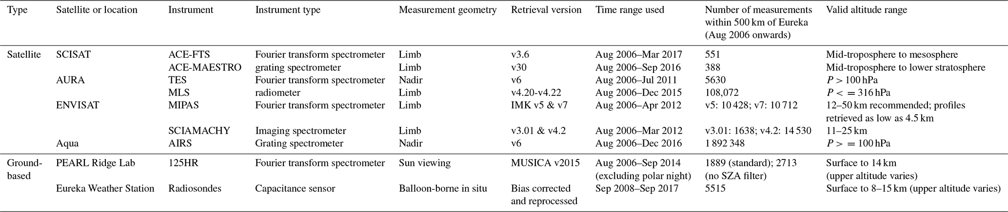
This section presents the water vapour datasets from Eureka ground-based instruments and Eureka-coincident satellite instruments that are used in this study. Table 1 summarizes the available datasets and notes the technique, retrieval version, and how often measurements are taken. Figure 1 illustrates the temporal availability of atmospheric water vapour measurement from each instrument. Figure 2 illustrates the vertical ranges of the datasets.

2.1 Radiosondes
Radiosondes are launched by the EWS twice a day (11:15 and 23:15 UT) using hydrogen-filled balloons. Occasionally, additional radiosondes are launched at other times of day for campaigns. The balloons typically reach the middle of the stratosphere (i.e. 30–33 km) before bursting.
The EWS used Vaisala-built RS92 radiosonde models during the timeframe examined in this study. These sensors are widely used by meteorological stations around the world. RS92 relative humidity (RH) measurements are made using thin-film capacitance sensors. The variable of interest for this study is the volume mixing ratio (VMR) in parts per million by volume (ppmv). RH measurements from the radiosondes can be converted to mixing ratio using
where RH is the relative humidity, T and P are the temperature and pressure, respectively, at a given altitude (z), and es is the temperature-dependent saturation vapour pressure of water vapour with respect to liquid water. The es equation of Hyland and Wexler (1983) is used for consistency with Vaisala humidity measurement calibration (Miloshevich, 2006).
As the balloon rises through the atmosphere, there comes a point where the humidity sensor can no longer report a meaningful value. Limiting the radiosonde humidity measurements to below the tropopause height (TPH) or a typical tropopause value usually ensures that only physically meaningful observations are used; however, this potentially removes valid and useful information.
Eureka radiosonde humidity profiles often have clear structure and information about water vapour above the tropopause, which is typically between 8 and 12 km. Miloshevich et al. (2009) found that the tropopause is not a limiting factor for RS92 humidity measurements and reported close agreement between bias-corrected radiosonde and frost-point hygrometer (FPH) profiles at temperatures below −70 ∘C and below mixing ratios of 5 ppmv. They recommended limiting radiosondes to pressures greater than 100 hPa during daytime and 75 hPa at night. The mean altitude at which the atmosphere above Eureka has a pressure of 100 hPa is 16.01 km (σ=0.47 km) based on radiosonde measurements between 1961 and 2017. We limit radiosonde humidity measurements to altitudes below 15 km for this study as a quality control measure.
RS92 humidity measurements are also known to be affected by solar heating and low-temperature calibration error dry biases as well as errors due to sensor response lag (Vömel et al., 2007a; Miloshevich et al., 2009). The dry bias caused by solar heating of the sensor is not significant in Eureka during winter due to the lack of sunlight; however, it can affect measurements during the sunlit portion of the year. The calibration error and time-lag error affect low-temperature measurements and are relevant for Eureka conditions. To correct for known biases in a consistent, transparent, and well-documented manner, Eureka radiosonde measurements were processed with software developed by the GCOS Reference Upper-Air Network (GRUAN), described by Dirksen et al. (2014). Eureka is not a formal GRUAN-participating site, and the data are not a formal GRUAN data product; however, available raw Eureka radiosonde measurement files were processed by the GRUAN team for use in this study. This processing also calculates uncertainties for reported values and recovers flight details (e.g. latitude and longitude). Only raw files between 3 September 2008 and 7 October 2017 were available for processing. Minor gaps within that timeframe exist. In total, 5515 radiosonde profiles which were processed using GRUAN methodologies are available for Eureka. They were quality control-filtered to remove any profile with “rejected” status.
In the troposphere, the uncertainty of Eureka radiosonde water vapour mixing ratio profiles is typically 3 % to 5 %. In the LMS, the uncertainty varies from profile to profile, ranging from 3 % to above 50 %. Uncertainty in the water vapour mixing ratio, calculated by propagating uncertainties in Eq. (1) by quadrature, is dominated by the relative humidity uncertainty. Temperature measurement uncertainties are typically a few tenths of a degree. Pressures similarly have uncertainties on the order of tenths of a hectopascal. There are occasionally thin dry layers in the middle troposphere that have larger humidity uncertainty. These profile elements are kept. If there are sections of the profile larger than 500 m in the troposphere with high uncertainty values, the entire profile is filtered out.
In the lower stratosphere, the profile reaches a point where the uncertainty increases rapidly. This point changes from profile to profile. We limit each individual water vapour profile to the altitude where this rapid increase in uncertainty occurs by finding where the uncertainty first reaches 20 %. This is typically a few kilometres above the tropopause. Thus, each radiosonde profile has a different altitude range depending on the height reached by the balloon and the uncertainty of the measurements. The mean altitude reached by the filtered profiles is 11.3 km (σ=4.4 km).
Once launched, radiosonde balloons drift away from the site due to winds. The radiosondes used in this study stayed within a mean distance of 29.8 km (σ=16.5 km) from Eureka while being under 15 km altitude. The mean time to reach 15 km altitude was 54.4 min (σ=6.2 min).
2.2 PEARL 125HR
The Bruker-made IFS 125HR FTIR spectrometer used for this study is located at the Ridge Lab. Installed in July 2006, the 125HR records high-resolution (0.0035 cm−1) mid-infrared (MIR) solar absorption spectra in the framework of the Network for the Detection of Atmospheric Composition Change (NDACC; Batchelor et al., 2009). Because this technique relies on sunlight, measurements require clear-sky conditions. Due to PEARL's 80∘ N latitude, there are no 125HR measurements from mid-October to mid-February (i.e. during polar night). Even in midsummer, the high-latitude FTIR spectrometer measurements occur at a relatively large solar zenith angle (SZA). The minimum SZA at Eureka is 56.5∘. This measurement geometry means that the 125HR typically samples the atmosphere south of the Ridge Lab. During the 24 h sunlight of the polar day, during the high Arctic summer, the Sun's position is north of the instrument during what is usually night. However, 125HR measurements are not made overnight due to on-site operator limitations and the lack of an automated shutdown trigger in the case of problematic weather.
The 125HR water vapour dataset used in this study was produced using the retrieval technique summarized in Schneider et al. (2012) and Barthlott et al. (2017) as part of the Multi-platform remote Sensing of Isotopologues for investigating the Cycle of Atmospheric water project (MUSICA, 2019). MUSICA uses the existing NDACC FTIR spectrometer observations to produce precise and accurate measurement of water vapour isotopologues. This process applies an optimal-estimation technique based on Rodgers (2000) and the PROFITT retrieval code of Hase et al. (2004) using a combination of strong and weak absorption features on a logarithmic scale. The accuracy of the MUSICA water vapour profiles is about 10 % (Schneider et al., 2016). The sensitivity of the retrieval to the atmosphere (i.e. the sum of the averaging kernel rows) varies seasonally due to the dependence on the SZA. The retrieval is typically sensitive throughout the troposphere (i.e. sensitivity above 0.9), and there is some sensitivity in the lower stratosphere (e.g. sensitivity above 0.5). The MUSICA retrieval's sensitivity to the lower stratosphere is maximum during March, which is also when ACE coincidences occur with Eureka. The mean degree of freedom for signal (DOFS) of the Eureka MUSICA retrievals is 2.9. The vertical sensitivity of the MUSICA retrieval is illustrated by Figs. 2, 3, and 4 in Barthlott et al. (2017), and that for the MUSICA retrieval at the Eureka site is illustrated by Fig. 4 in Weaver et al. (2017).
MUSICA ground-based FTIR products nominally exclude measurements recorded at SZAs greater than 78.5∘. This filter has been removed for this study. Due to Eureka's high-latitude location, this filter removes all measurements between February and the end of March as well as between September and mid-October. A study of the MUSICA water vapour total column dataset derived from the PEARL 125HR showed that the SZA limit was likely unnecessarily strict, as agreement did not change between the 125HR and other instruments when the SZA limit was relaxed (Weaver et al., 2017). Standard quality control of the MUSICA dataset, which was applied to the data used here, is described in detail by Barthlott et al. (2017).
2.3 ACE on SCISAT
The Canadian Space Agency's (CSA's) SCISAT was launched into a high-inclination (74∘) 650 km altitude Earth orbit on 12 August 2003. This orbit enables limb-viewing measurements over the polar regions as well as other latitudes. There are two primary ACE instruments aboard SCISAT, the ACE Fourier transform spectrometer (ACE-FTS), and the ACE Measurement of Aerosol Extinction in the Stratosphere and Troposphere Retrieved by Occultation (ACE-MAESTRO). They share a sun tracker. ACE solar occultation limb-viewing observations involve keeping the sun tracker pointed at the Sun as the satellite approaches a sunrise or sunset during its orbit and taking sequences of atmospheric and exoatmospheric absorption spectra.
Coincidences between ACE and Eureka occur during the months of February, March, September, and October. 348 out of 551 coincidences between ACE and Eureka between August 2006 and March 2017 occurred during February and March.
2.3.1 ACE-FTS
ACE-FTS is an FTIR spectrometer built by ABB, Inc. It acquires spectra between 750 and 4400 cm−1 at a resolution of 0.02 cm−1 (Bernath et al., 2005). This series of measurements, taken every 2 s, is used to retrieve trace gas profiles between the mid-troposphere and 150 km with a vertical resolution ranging between 3 and 4 km (Boone et al., 2013). This technique has a horizontal resolution of ∼300 km (Bernath, 2017).
This study uses ACE-FTS v3.6 data provided on the 1 km altitude grid in the water vapour mixing ratio (ACE, 2019). Measurements with quality control flags identifying outliers, high percentage of errors, or instrument and/or processing errors were filtered out, following recommendations in Sheese et al. (2015). The water vapour retrieval is limited to altitudes between 5 and 100 km.
The validation of an earlier version (v2.2) of ACE-FTS (and to a limited extent, ACE-MAESTRO) water vapour retrievals was examined by Carleer et al. (2008). They concluded that ACE-FTS measurements provide accurate H2O measurements in the stratosphere (better than 5 % from 15–70 km) but expressed no firm conclusions about its water vapour measurements in the upper troposphere. Comparisons to FPH measurements showed a possible small dry bias in ACE-FTS measurements at altitudes near 10 km.
Sheese et al. (2017) examined the current ACE-FTS v3.6 H2O product (as well as other molecules) by comparing it with co-located Michelson Interferometer for Passive Atmospheric Sounding (MIPAS) and Microwave Limb Sounder (MLS) measurements by hemisphere. Correlations between ACE-FTS and MLS were observed to be greater than between ACE-FTS and MIPAS. Their analysis examined stratospheric altitudes, where a mean relative difference in the ACE-FTS water vapour product was observed above 16 km, ranging from −12 % to 2 %. In addition, tight coincidence criteria of 15 min and 25 km were applied to examine agreement near the hygropause. A mean dry bias of 20 % was observed in ACE-FTS profiles relative to MIPAS v5 and MLS v3.3 or 3.4 at 13 km altitude.
2.3.2 ACE-MAESTRO
ACE-MAESTRO is a dual spectrometer with a wavelength range of 285–1015 nm and a resolution of 1.5–2.5 nm (McElroy et al., 2007). The ACE-MAESTRO water vapour retrieval algorithm produces profiles with an approximate vertical resolution of 1 km and is described by Sioris et al. (2010), with updates described in Sioris et al. (2016). Water vapour profiles are retrieved from ACE-MAESTRO optical depth spectra (ACE, 2019). The tangent height registration of the optical depth spectra relies on matching simulated O2 slant columns obtained from air density profiles, based on ACE-FTS temperature and pressure, with slant columns observed by ACE-MAESTRO using the O2 A band. The water vapour profiles are retrieved on an altitude grid that matches the vertical sampling. Within 500 km of Eureka, ACE-MAESTRO water vapour profiles include altitudes ranging between 4 and 25 km.
The ACE-MAESTRO dataset is sparser than the ACE-FTS dataset for two main reasons. ACE-MAESTRO pointing determination requires the existence of ACE-FTS data, so the available ACE-MAESTRO occultation events are a subset of the ACE-FTS occultations. In addition, ACE-MAESTRO ozone is a necessary input to the ACE-MAESTRO water vapour retrieval. The ACE-MAESTRO ozone retrieval fails occasionally, causing most of the measurements missing from the ACE-MAESTRO water vapour product relative to the ACE-FTS product.
2.4 Aqua
The US National Aeronautic and Space Administration (NASA) launched the Aqua satellite into a 705 km altitude Sun-synchronous near-polar orbit on 4 May 2002. Aqua's orbit has a 13:30 equatorial crossing time and an inclination of 98.2∘. It is part of the A-train constellation of Earth observation satellites. The primary mission of Aqua instruments is to study the atmospheric component of the global water cycle (Parkinson, 2003).
2.4.1 AIRS
The Atmospheric Infrared Sounder (AIRS) instrument is a hyperspectral thermal infrared grating spectrometer aboard Aqua. Its detector observes Earth-emitted radiance from a nadir orientation using 2378 channels between 3.7 and 15.7 µm. AIRS acquires an enormous number of measurements, collecting about 3 million spectra per day (Chahine et al., 2006).
AIRS water vapour retrievals have been used to study processes such as the water vapour feedback (Dessler et al., 2008), to evaluate climate models (Pierce et al., 2006), and to improve numerical weather forecasting (Chahine et al., 2006). AIRS aims to produce dense global measurements of temperature and humidity at an accuracy comparable to radiosondes. This study uses Level 2 AIRS retrieval v6 data, described in detail by Susskind et al. (2003, 2014). The standard temperature product contains 28 pressure levels, while the standard water vapour product has 15 pressure levels from 1100 to 50 hPa (e.g. between the surface and approximately 20 km in altitude near Eureka; AIRS, 2019).
Only altitudes that meet the “best” level of quality are used for this study, following the guidelines in the AIRS v6 user guide (Olsen et al., 2017). The altitude range for which AIRS profiles are available varies significantly, with fewer passing the quality control filter at low-tropospheric altitudes. The AIRS retrieval is insensitive to water vapour layers with less than 0.01 mm of integrated water vapour. This approximately translates to water vapour abundances less than 15 ppmv (Olsen et al., 2017), typically affecting profile elements above 15 km near Eureka. AIRS is also limited to altitudes with pressures greater than 100 hPa and has diminishing sensitivity at altitudes with pressures less than 300 hPa (approximately 9 km near Eureka; Olsen et al., 2017). As mentioned in the discussion of the radiosondes' altitude range, 100 hPa occurs at approximately 16 km in altitude above Eureka. The relative abundance of AIRS profiles ensures that measurements are nonetheless available for comparisons.
2.5 Aura
NASA's Aura satellite was launched into a near-polar Sun-synchronous 705 km orbit on 15 July 2004. It is part of the A-train constellation of Earth observing satellites, orbiting 15 min behind Aqua. Aura's orbit has a 98.2∘ inclination and an equatorial crossing time around 13:45 LST (local solar time). Instruments aboard Aura, such as the MLS and Tropospheric Emission Spectrometer (TES), study atmospheric chemistry and dynamics.
2.5.1 MLS
MLS measures radiation emitted from the atmosphere from a limb-viewing geometry. The atmosphere is scanned twice each minute as the satellite progresses through an orbit that offers nearly global coverage, between 82∘ N and 82∘ S. MLS measurements have been used to assess ACE as well as other satellite measurements, e.g. in Hegglin et al. (2013) and Sheese et al. (2017). This study uses MLS v4.2 data (MLS, 2019).
MLS water vapour profiles are vertically resolved at pressures less than 383 hPa, with a vertical resolution ranging between 1.3 and 3.6 km from 316 to 0.22 hPa (Livesey et al., 2016). At Eureka, MLS's lower altitude limit of 316 hPa corresponds to altitudes near 8 km. MLS water vapour profiles agree within 1 % of FPH measurements in the stratosphere, i.e. at p < 100 hPa (Hurst et al., 2014). Hurst et al. (2016) showed that agreement between MLS v4.2 and the FPH measurements began to diverge in 2010 at a rate of approximately 1 % per year. At 215 and 316 hPa, MLS v1.5 was observed to have a dry bias of 11 % to 23 % relative to 10 geographically dispersed FPH measurement sites (Vömel et al., 2007b).
2.5.2 TES
TES is an FTIR aboard Aura that observes emitted radiance between 650 and 3050 cm−1 spectral resolution of 0.10 cm−1 when observing in nadir mode and 0.025 cm−1 in limb-viewing mode (Beer et al., 2001). Limb-scanning measurements were performed only until May 2005. The TES water vapour retrieval uses nadir observations, which have a footprint of 5 km by 8 km. Routine measurements involve a series of observations continuously for 16 orbits (26 h).
Measurements are only available near Eureka's high Arctic latitude until September 2008. The latitudinal range of TES measurements was limited to latitudes between 50∘ S and 70∘ N in summer 2008 to conserve instrument life (Herman and Osterman, 2014). Measurements were further limited to between 30∘ S and 50∘ N in spring 2010. However, high-latitude measurements were taken in July 2011 as part of a special observation set.
TES retrieval v6 is used for this study (TES, 2019). It is based on an optimal-estimation non-linear least-squares approach described by Bowman et al. (2006). The vertical information content of TES profiles varies; retrievals with fewer than three DOFSs are filtered out. In the subset of measurements examined in this study, TES DOFSs range between 3.0 and 5.2. At polar latitudes, the vertical resolution is approximately 11.6 km between 400 and 100 hPa and 6.0 km between 1000 and 400 hPa (Worden et al., 2004).
Comparisons between TES v5 water vapour and global radiosonde measurements have shown a wet bias of 15 % in the middle troposphere (Herman and Kulawik, 2013). Shephard et al. (2008) compared TES water vapour v3 with radiosondes, finding a wet bias in TES retrievals of between 5 % in the lower troposphere and 15 % in the upper troposphere.
2.6 EnviSat
The European Space Agency (ESA)'s Environmental Satellite (EnviSat) was a large platform for Earth observation instruments. Launched into a polar orbit on 1 March 2002, with an inclination of 98.5∘ and an equatorial crossing time of 10:00 LMT (local mean time). Observations from its 10 instruments ended in April 2012. On board were two atmospheric limb sounders, the MIPAS and the Scanning Imaging Absorption Spectrometer for Atmospheric CHartography (SCIAMACHY). Measurements for a decade taken by MIPAS and SCIAMACHY have been widely used to study atmospheric composition and are often used in comparisons to other limb sounders.
2.6.1 MIPAS
MIPAS is an FTIR spectrometer that observes mid-infrared atmospheric emission from a limb-viewing geometry (Fischer et al., 2008). The spectral resolution of MIPAS was reduced from 0.025 to 0.0625 cm−1 in 2004 due to technical problems. The timeframe examined in this study, 2006–2012, is entirely during the reduced spectral resolution period. This measurement mode has improved spatial resolution. In polar regions, the nominal tangent altitude spacing is 1.5 km in the UTLS region.
This study uses MIPAS retrieval v5 and v7 from the Institute of Meteorology and Climate Research (IMK; MIPAS, 2019). Both retrieval versions cover the same temporal range. This retrieval technique is described by von Clarmann et al. (2009) and uses Tikhonov regularization. In the UTLS, the profiles are provided on a 1 km grid. At 10 km, the vertical resolution (v5) is 3.3 km, and the horizontal resolution is estimated to be 206 km (von Clarmann et al., 2009). Quality control filtering is applied according to recommended values. MIPAS water vapour data are recommended for use only above the 12 km altitude. However, in this study all available altitudes provided in the official data release are used. MIPAS water vapour profile retrievals reach altitudes as low as 5 km.
Stiller et al. (2012) compared an earlier version of the MIPAS IMK retrieval (v4) with cryogenic frost-point hygrometer (CFH) measurements of water vapour profiles during the Measurements of Humidity in the Atmosphere and Validation Experiments (MOHAVE) campaign near Pasadena, California, in October 2009. Above 12 km, MIPAS showed agreement within 10 %. Results suggest that MIPAS v4 water vapour might have a 20 %–40 % wet bias around 10 km.
2.6.2 SCIAMACHY
SCIAMACHY is an imaging spectrometer that has limb, nadir, and occultation viewing modes (Bovensmann et al., 1999). Limb measurements of scattered sunlight are the basis for the Institut für Umweltphysik (IUP) v3.01 and v4.2 water vapour retrievals used in this study (SCIAMACHY, 2019). Both retrieval versions cover the same temporal range. It is based on the optimal-estimation approach described by Rodgers (2000) using a first-order Tikhonov constraint. The vertical resolution is approximately 3 km. The retrieval calculates a scaling factor for the tropospheric water vapour profile; altitudes below 10 km are not recommended for use and are not used here. The details of this retrieval are described in Weigel et al. (2016) for v3.01. For v4.2 several changes were implemented; first of all, these were to improve the aerosol correction and the vertical resolution. Additionally, v4.2 uses all appropriate SCIAMACHY measurements, and v3.01 uses only a subset. One issue for limb sensing is the number of cloud free scenes. This is limited by the sampling approach, which was constrained by the data rate available on Envisat.
Weigel et al. (2016) compared MIPAS v3.01 to MIPAS v5, MLS v3.3, and other satellite datasets in 30∘ latitudinal bands. Results showed that SCIAMACHY limb measurements between 10 and 25 km in altitude were reliable between 11 and 23 km and accurate to about 10 % between 14 and 20 km. Below 14 km, differences with other datasets increase to up to 50 %, showing a possible SCIAMACHY v3.01 wet bias, which is most pronounced in the tropics and least pronounced in the polar latitudes.
Water vapour profiles from ACE-FTS, ACE-MAESTRO, AIRS, MIPAS, MLS, SCIAMACHY, and TES were compared with Eureka radiosonde and PEARL 125HR measurements following the methodology described below. Two ground-based reference measurements are used in this study to maximize comparisons with available satellite measurements. The radiosondes provide profiles at high vertical resolution; however, they had few or no coincidences with MIPAS, SCIAMACHY, and TES. The 125HR, while having more limited vertical resolution, had coincident measurements with all satellite datasets used in this study.
3.1 Method
Coincident profile measurements have been compared using difference and correlation plots. Absolute differences and percent relative differences are calculated using
where X is the satellite measurement and Y is the reference measurement, e.g. 125HR or radiosondes.
To show the overall agreement observed between the measurements, the absolute and percentage means of coincident profile differences are calculated, i.e. using
and
Altitude ranges for which there are measurements available vary for each contributing matched pair of profiles, resulting in a variable number of profiles contributing to comparisons at each altitude. The number of contributing matches at each altitude level is reported in the comparison figures.
In addition to showing profile comparisons, comparisons at specific representative altitudes are presented. These illustrate the extent of the variability in the overall mean agreement between the datasets.
A minimum number of 15 coincidences is required, i.e. N≥15, for results to be reported and shown in the tables and figures. This aimed to balance the reality that there are limited number of coincidences available and the need to ensure that there are a meaningful number of comparison results available at each altitude.
3.1.1 Coincidence criteria
A 3 h temporal coincidence criterion was used for all comparisons and applied in two ways. Firstly, if multiple coincidences were found within this interval, only the closest pair was kept. Each pair of coincident measurements is thus independent of others, contributing to the overall assessment of different measurement techniques. This method often results in a smaller time difference between measurements than is otherwise permitted by the criterion. The comparisons were also performed using all possible coincidences within this criterion. While increasing the number of matches, in some cases significantly, the observed agreement between instruments was similar to that for the first method, which is summarized in Tables 2 and 3. Results using the first method are discussed below. Results of comparisons where all possible coincidence pairs are used are available in Supplement Tables S1 and S2.
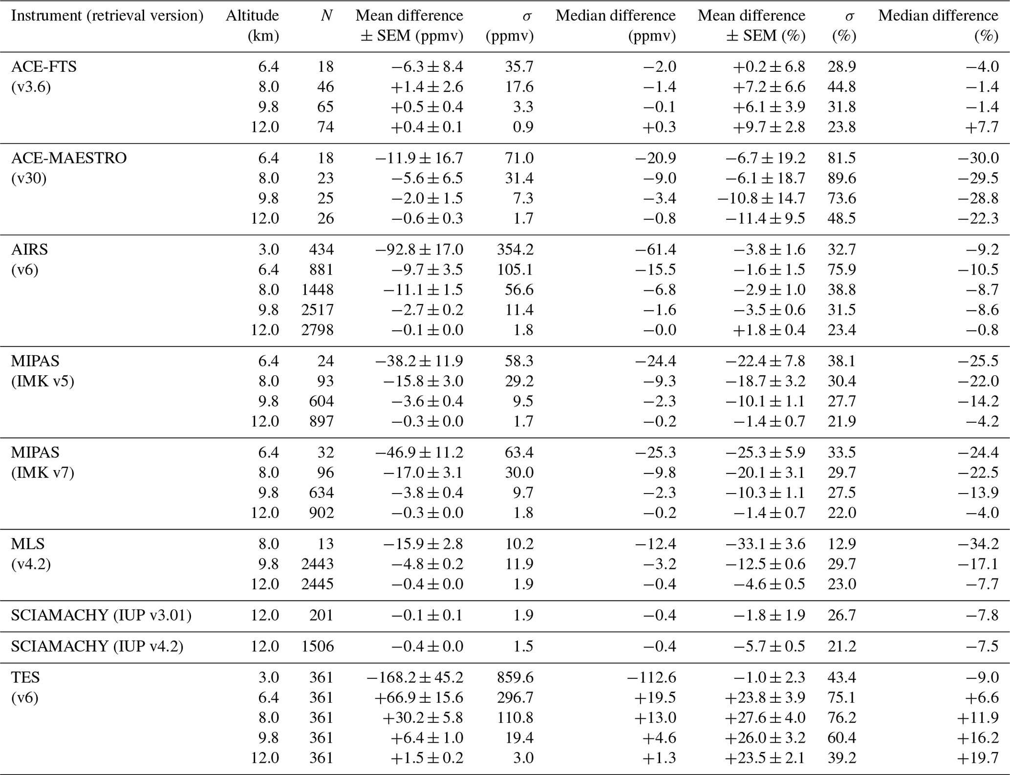
Table 2Summary of satellite vs. 125HR comparison results. SEM refers to the standard error in the mean, i.e. .
A 500 km spatial coincidence criterion was also applied. The spatial criterion is similar in scale to the horizontal area covered by a limb-viewing satellite measurement. When calculating the distance between PEARL and an ACE observation, the 30 km (calculated geometrically) tangent height of the ACE measurement was used as the satellite measurement's position. This approach has been used for validation, e.g. in Fraser et al. (2008).

Figure 2Vertical range of datasets used in this study. Colour range showing the number of profiles at each altitude level shows the log(N).
The difference in measurement geometries, and the long path of a limb-viewing measurement in particular, can result in ACE-FTS measuring a different air mass than the 125HR and radiosondes. Figure 3 illustrates the variation in water vapour abundances in the region around Eureka using AIRS measurements at 400 hPa (corresponding to altitudes between 6.1 and 7.5 km, with a mean altitude of 6.7 km and a standard deviation of 0.2 km) for two sample months, March and July, in a representative year (2015). Variability in the water vapour abundances in the region around Eureka is seen to be larger in the summer than in the winter. October resembles the results shown for March.
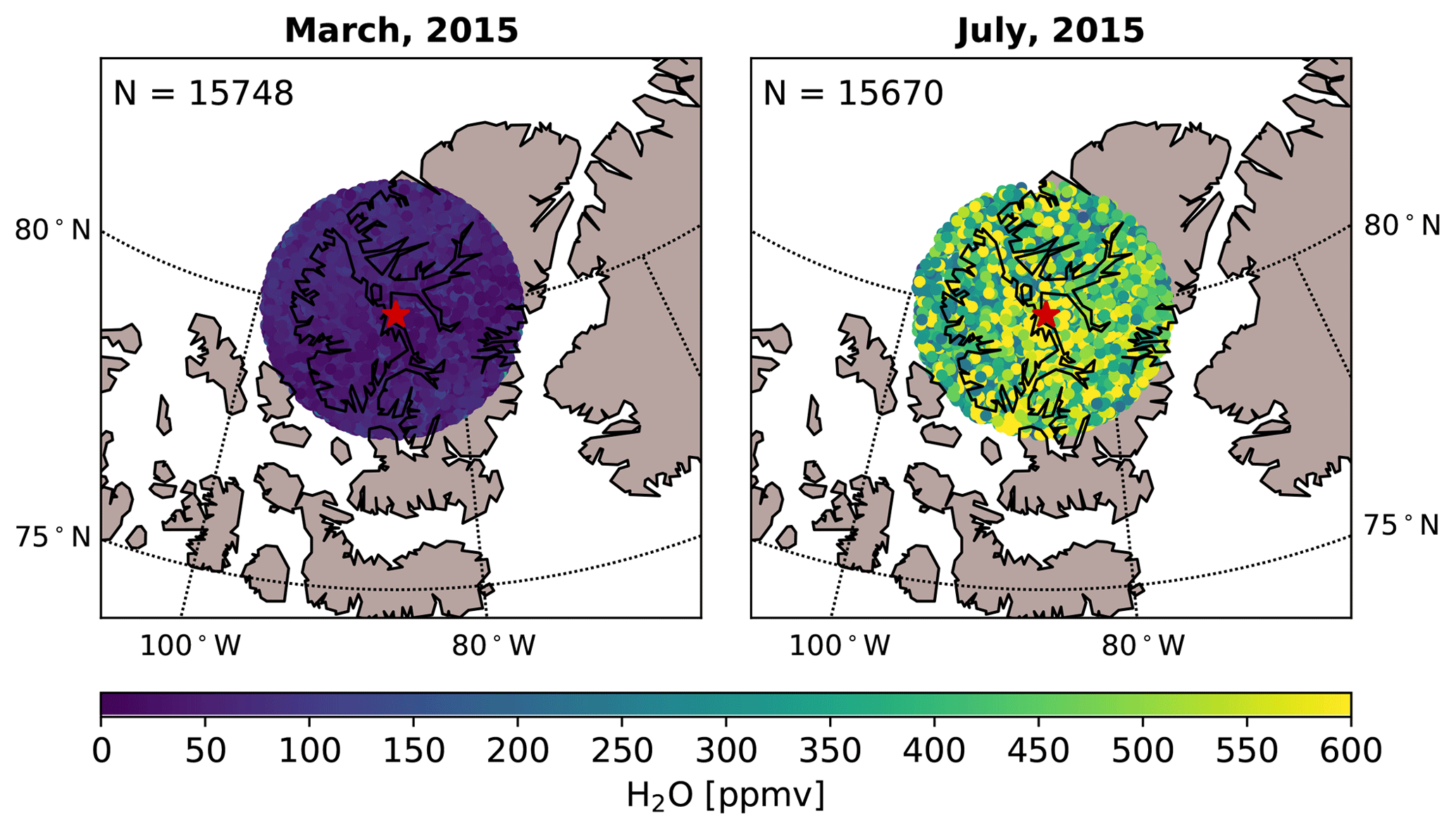
Figure 3AIRS water vapour abundances at 400 hPa near Eureka (indicated by the red star) in March and July 2015.
3.1.2 Smoothing
When comparing satellite profiles with the PEARL 125HR, the comparison instrument's profile was smoothed by the MUSICA averaging kernel of the 125HR measurement to account for the vertical resolution differences between the instruments. The procedure for smoothing followed Rodgers and Connor (2003):
where xa is the MUSICA a priori profile, x is the comparison instrument profile, and A is the averaging kernel matrix. Since the MUSICA water vapour retrievals are performed on a logarithmic scale, the smoothed profile is calculated using
where x, xa, and A are in loge space.
Before smoothing, the satellite profile was interpolated to the MUSICA retrieval grid, and the MUSICA a priori profile was used to fill gaps in the comparison profile (e.g. altitudes beneath the lower limit of satellite measurements). After smoothing, altitudes for which there were no original data were removed. Altitude-specific comparisons between satellite measurements and the FTIR are thus presented on the MUSICA retrieval grid, e.g. 6.4, 8.0, and 9.8 km.
When comparing satellite measurements to the radiosonde profiles, radiosonde profiles were smoothed using the satellite's averaging kernels where possible, i.e. for SCIAMACHY and TES, following the same procedure described for the 125HR. MIPAS retrievals do not use an a priori profile, so the smoothed radiosonde profile is calculated using
In the cases of ACE-FTS, ACE-MAESTRO, AIRS, and MLS, the radiosonde profiles have been smoothed using Gaussian weighting functions with a full width at half maximum (FWHM) that approximates the vertical resolution of the satellite measurement. This procedure is used because ACE instruments do not have averaging kernels. MLS has an averaging kernel for use in the polar regions; however, the user's guide states that the use of the water vapour averaging kernel at the lowest valid altitude levels (i.e. lower stratosphere at 316 and 262 hPa) is not recommended (Livesey et al., 2016). Since these altitudes are of particular interest to this study, the MLS averaging kernels are not suitable. AIRS also has averaging kernels distributed in supplementary data files; however, the AIRS averaging kernels only capture the information added during the final physical retrieval but not the information extracted from the AIRS radiances during the neural network step. We use the width of the AIRS weighting functions to estimate a Gaussian smoothing width that generally overestimates the amount of smoothing. Thus, weighting functions are used in these cases as a reasonable approximate method of smoothing the vertical resolution of these profiles.
To create weighting functions, first, Gaussian functions are calculated using
where FWHM is the full width at half maximum, z is the new low-resolution grid point, and zo values are the original altitude levels.
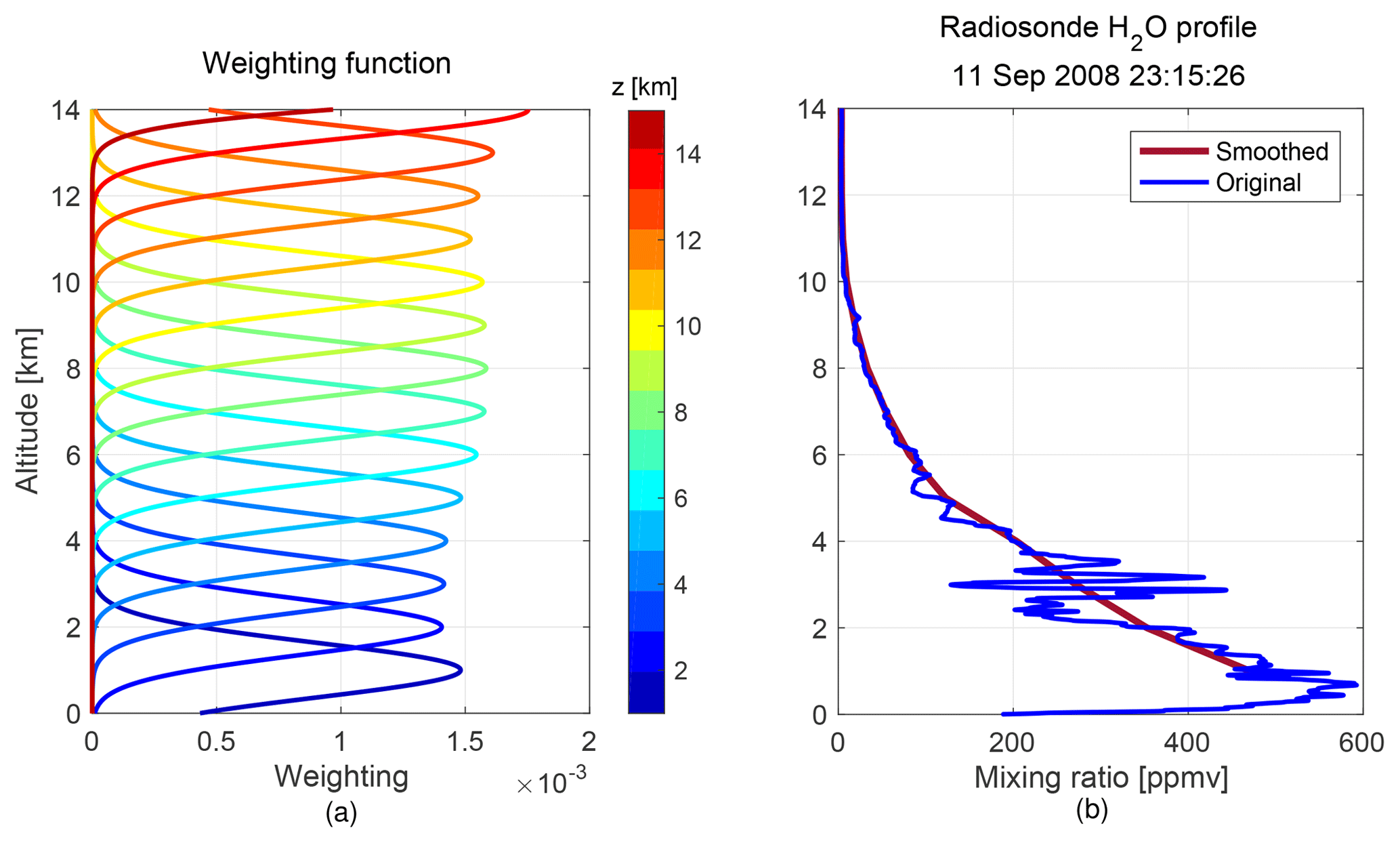
Figure 4(a) shows an example of weighting functions used to smooth the radiosonde profiles to ACE-FTS vertical resolution. (b) shows the corresponding radiosonde profile, both measured (blue line) and after smoothing (maroon line), with the weighting function shown in (a).
Weighting functions were calculated by sampling the GF at the original radiosonde measurement altitude levels and normalizing the GF so that the total weight assigned to all profile elements is equal to 1. The weighting functions are different for each pair of coincident profiles because the vertical sampling of each radiosonde profile varies.
Lastly, the vertical resolution of radiosonde water vapour VMR profiles was downgraded using the weighting functions (wf's):
An example of weighting functions used to align the radiosonde measurement with the approximate vertical resolution of ACE-FTS is shown in Fig. 4a. Figure 4b shows an example of a radiosonde profile before and after smoothing. Weighting functions with a FWHM equal to 3.0 km have been used to approximate the vertical resolution of ACE-FTS, while comparisons to ACE-MAESTRO, AIRS, and MLS used weighting functions with a FWHM of 1.0 km.
3.2 Comparison results
Differences between individual coincident profiles were calculated. The means of those differences are presented. When reporting a mean agreement in the text, ± values refer to the standard error in the mean (SEM). Profile results are presented as well as comparison results at select altitude levels. Results between the satellites and the 125HR at 6.4 km are highlighted because the 125HR has very good sensitivity at that altitude, and this is near the lowermost altitude reached by the ACE measurements. Comparison results between the satellites and the radiosondes are highlighted at 10 km because radiosondes have sensitivity at that altitude; this is the lowermost altitude of other comparison studies, e.g. Sheese et al. (2017), and it is near the lower limit of many satellite datasets.
Some combinations of instruments did not have significant overlap in time, location, or vertical sensitivity. MIPAS and the radiosondes had no coincidences due to a mismatch in the time of day of the measurements as well as the quality control filtering. The temporal ranges of the TES and radiosonde datasets did not overlap. SCIAMACHY did not have any coincidences with the radiosondes unless the coincidence criterion was expanded to 6 h. Even then, only eight matches were found. SCIAMACHY and the 125HR had 201 coincidences; however, SCIAMACHY is limited to altitudes above 10 km, where the 125HR has limited sensitivity.
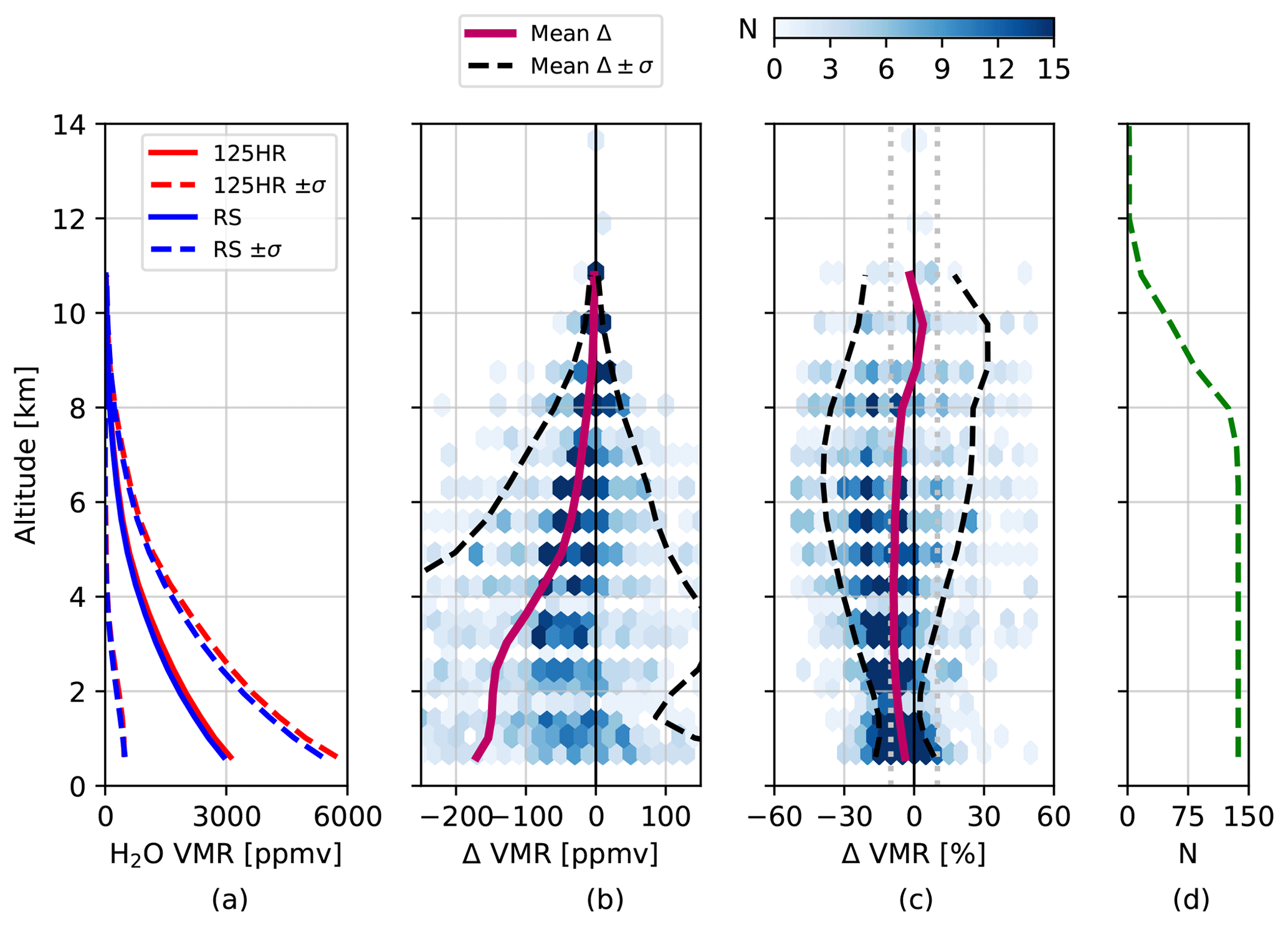
Figure 5Comparison between Eureka (GRUAN-processed) radiosonde and PEARL 125HR water vapour VMR. (a) Mean profiles (solid lines) ± the standard deviation (dashed lines). (b) Mean VMR difference (where X is radiosonde and Y is 125HR), using Eq. (4). (c) Mean percent difference, using Eq. 5. Grey dotted lines show ±10 %. In (b) and (c), the colour shading shows the number (N) of differences in each hexagon. (d) Number of coincident profile pairs at each altitude level. Note that comparisons are shown up to a maximum altitude of 11 km because the number of coincident pairs above that level do not meet the N > 15 threshold.
3.2.1 Ground-based reference measurements
As illustrated in Fig. 5, comparison between the 125HR and 137 coincident radiosonde profiles smoothed by 125HR averaging kernels shows agreement within 5 % between 8 and 14 km; the 125HR has a wet bias relative to the radiosonde profiles below 8 km of approximately 8 % (with closer agreement below 2 km). This is similar to the 6 % wet bias in the PEARL 125HR total columns relative to the Eureka radiosondes reported by Weaver et al. (2017). If all possible coincident pairs are used, rather than limiting comparisons to unique pairs, the number of contributing matches increases to 270 and the agreement is very similar.
3.2.2 ACE-FTS
Seventy-six pairs of coincident ACE-FTS and PEARL 125HR measurements show close agreement. Between 6 and 9 km agreement was within 9 ppmv and 13 %; between 8 and 14 km, agreement is within 1.4 ppmv and 10 %. Full profile comparisons are shown in Fig. 6. The mean difference of 18 coincident profiles at 6.4 km was ppmv (0.2±6.8 %); the time series of differences at 6.4 km are shown in Fig. 7. At 8.0 km, 46 coincident measurements agreed to within 1.4±2.6 ppmv (7.2±6.6 %). Differences at 8.0 km are illustrated in Supplement Fig. S1a. Correlation plots at 6.4, 8.0, and 9.8 km are presented in Fig. 8. Between 6 and 14 km, correlation coefficients (R) are between 0.48 and 0.80. Expanding the time criterion to 6 h nearly doubles the number of coincidences but results in similar agreement. Overall, relative to the 125HR, ACE-FTS shows a wet bias between 8 and 14 km of 7 % to 10 % and small differences of approximately 10 ppmv (2 %) near 6 km (Fig. 6).
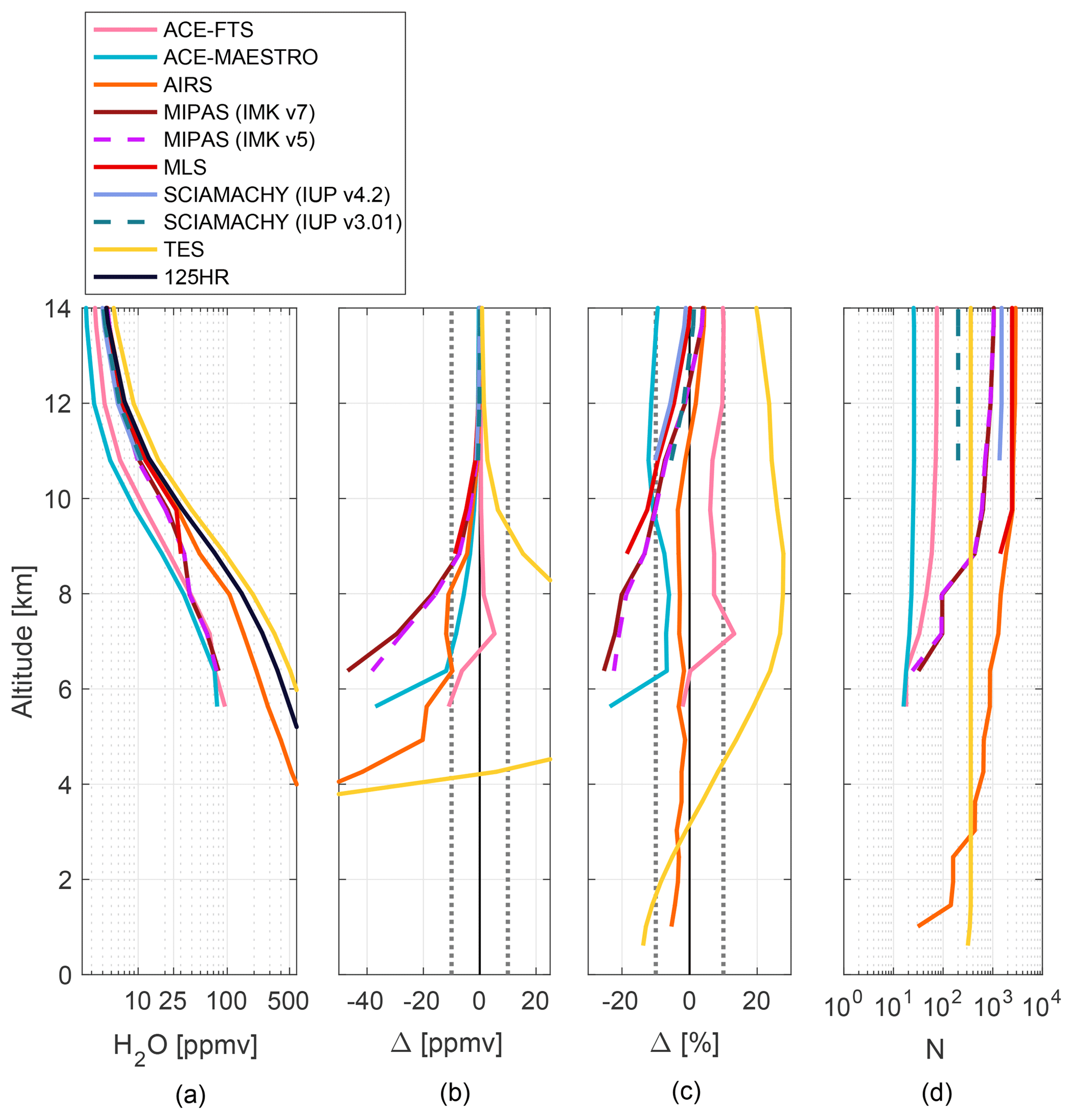
Figure 6Summary of differences between satellite measurements and PEARL 125HR. (a) The mean of profiles used in the comparison. (b) The mean VMR difference between the satellite profiles and the 125HR profiles, using Eq. (4). (c) The mean percent difference between the satellite profiles and the 125HR profiles, using Eq. (5). (d) The number of coincident profile pairs contributing to the comparison at each altitude level. Grey dotted lines in (b) and (c) show ±10 ppmv and ±10 %, respectively. Note that the x axes for panels (a) and (d) are on a log scale.
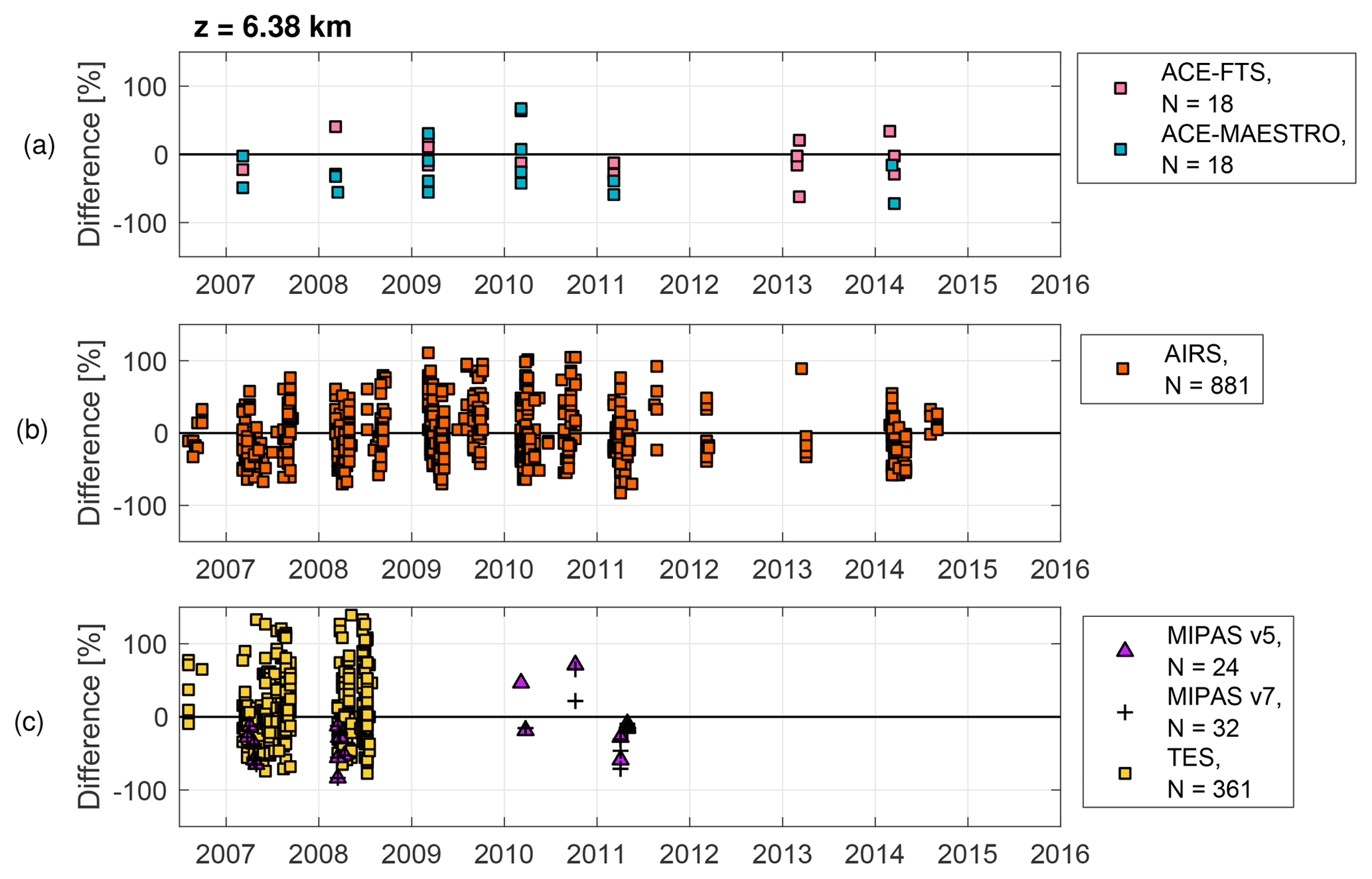
Figure 7Time series of percent differences between satellite and 125HR water vapour measurements at 6.4 km altitude for (a) ACE-FTS and ACE-MAESTRO, (b) AIRS, and (c) MIPAS and TES. In each case, the differences follow Eq. (3), where the satellite is X and the PEARL 125HR is Y.
One hundred eight coincident measurements were found between ACE-FTS and Eureka radiosondes. Profile differences are shown in Fig. 9 alongside results from other comparisons. These differences are also shown in Fig. S2, where ACE-FTS and ACE-MAESTRO comparison results are presented without other satellites for easier reading. Between 7 and 11 km, differences are within 6 ppmv (12 %). At 6 km, ACE-FTS and radiosonde profiles mean differences are ppmv (22.8±9.2 %). Differences at 10 km, ppmv ( %), are shown in Fig. 10a. Differences at 6 and 8 km are illustrated in the Supplement, Figs. S3a and S4a. Correlation plots at 6.4, 8.0, and 9.8 km are shown in Fig. 11. Correlation coefficients between 6 and 12 km range between 0.52 and 0.94.
In addition, comparisons have been done between the ACE-FTS results using AIRS as a reference. Differences at 10 km were ppmv ( %), increasing at lower altitudes to ppmv (39.6±4.3 %) at 6 km. Correlation coefficients for altitudes between 6 and 12 km were between 0.62 and 0.81. Correlation plots of ACE-FTS vs. AIRS at 6, 8, and 10 km are shown in Fig. 12.
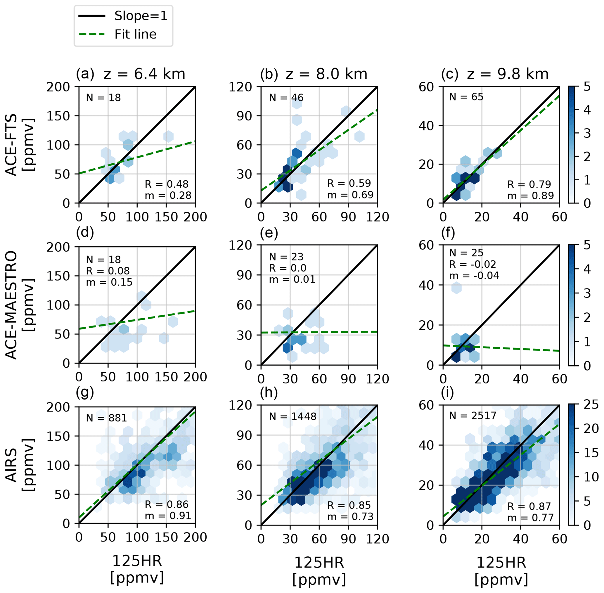
Figure 8Correlation plots for the ACE-FTS, ACE-MAESTRO, and AIRS satellite measurements vs. 125HR. The number of points in a given hexagon is colour-coded to show the density of the points. The scale at each end of a row shows the colour map used for that row. Solid black lines are 1:1 reference lines (i.e. slope =1); green dashed lines are lines of linear best fit. N is the number of coincident measurements for comparisons between the instruments at that altitude. R is the correlation coefficient. m is the slope of the best-fit line.
3.2.3 ACE-MAESTRO
Twenty-seven coincident measurements found between ACE-MAESTRO and the PEARL 125HR show agreement within 12 ppmv (7 %) between 6 and 8 km and within 3 ppmv (12 %) between 9 and 14 km. Overall, between 6 and 14 km, ACE-MAESTRO shows a dry bias of approximately 10 % relative to the 125HR (Fig. 6). Examining the agreement at specific altitudes in the middle and upper troposphere shows scatter around the zero line, illustrated in Figs. 7 and S1.
One hundred three coincident ACE-MAESTRO and radiosonde profiles were found with overlap between 5 and 11 km. Mean differences were large at 5 km, e.g. ppmv (123.4±71.1 %). Percent differences oscillate around −10 % between 7 and 10 km. At 8 km, ACE-MAESTRO had 90 coincidences with the radiosondes, with differences of ppmv ( %), shown in Fig. S4. At 10 km, absolute and relative mean differences were ppmv and %, respectively, shown in Fig. 10.

Figure 9Same as Fig. 6, but with a summary of differences between satellite measurements and Eureka radiosondes. A version of this figure with only the ACE-FTS and ACE-MAESTRO is available in the Supplement as Fig. S2.
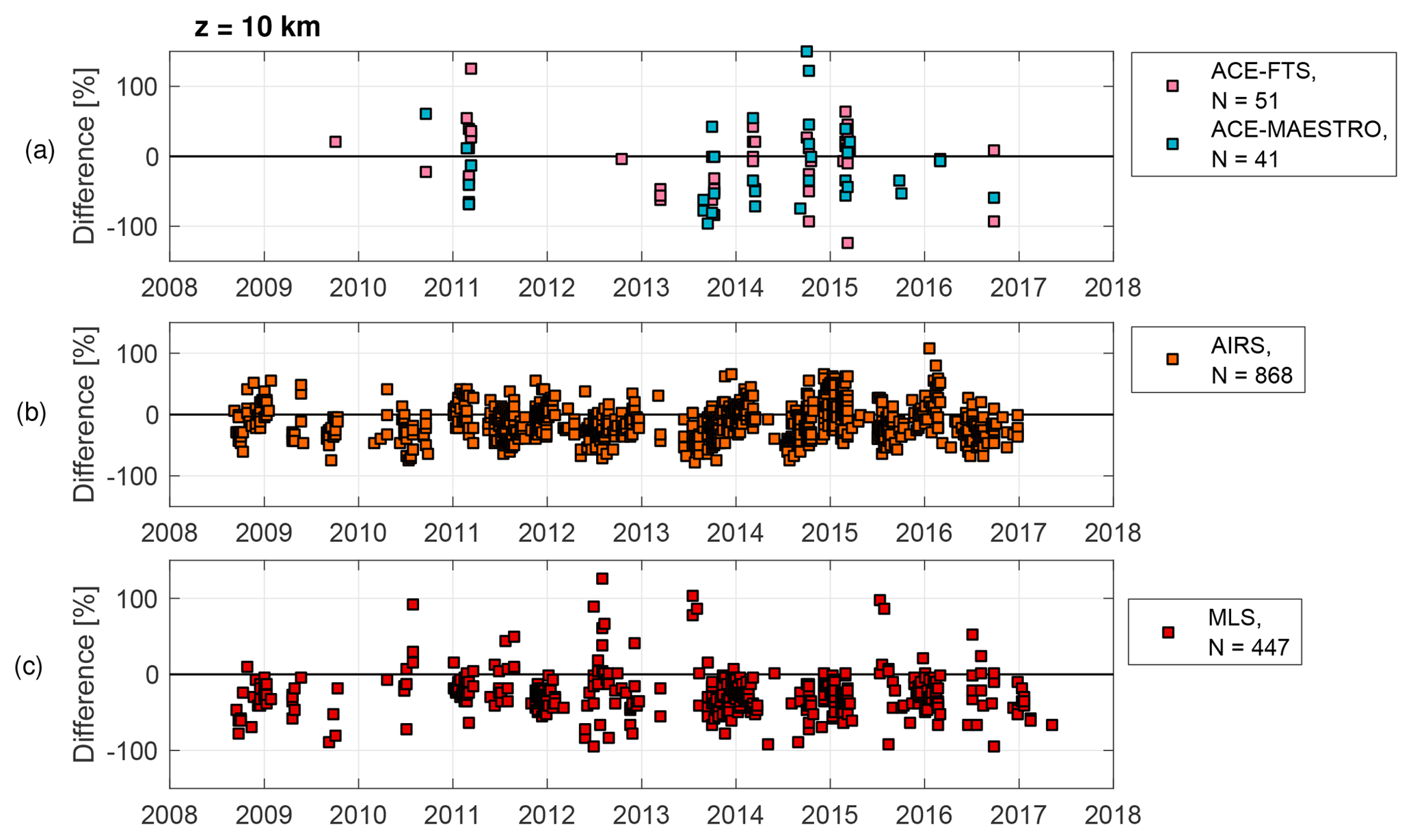
Figure 10Time series of percent differences between satellite measurements and the Eureka radiosondes at 10 km altitude for (a) ACE-FTS and ACE-MAESTRO, (b) AIRS, and (c) MLS. In each case, the differences follow Eq. (3), where the satellite is X and the Eureka radiosonde is Y.
In addition, comparisons have been done between the ACE-MAESTRO results using AIRS as a reference. Differences at 10 km were ppmv ( %), decreasing at lower altitudes to ppmv (69.9±13.5 %) at 6 km. Correlation coefficients for altitudes between 6 and 12 km were about 0.45. Correlation plots of ACE-MAESTRO vs. AIRS at 6, 8, and 10 km are presented in Fig. 12.
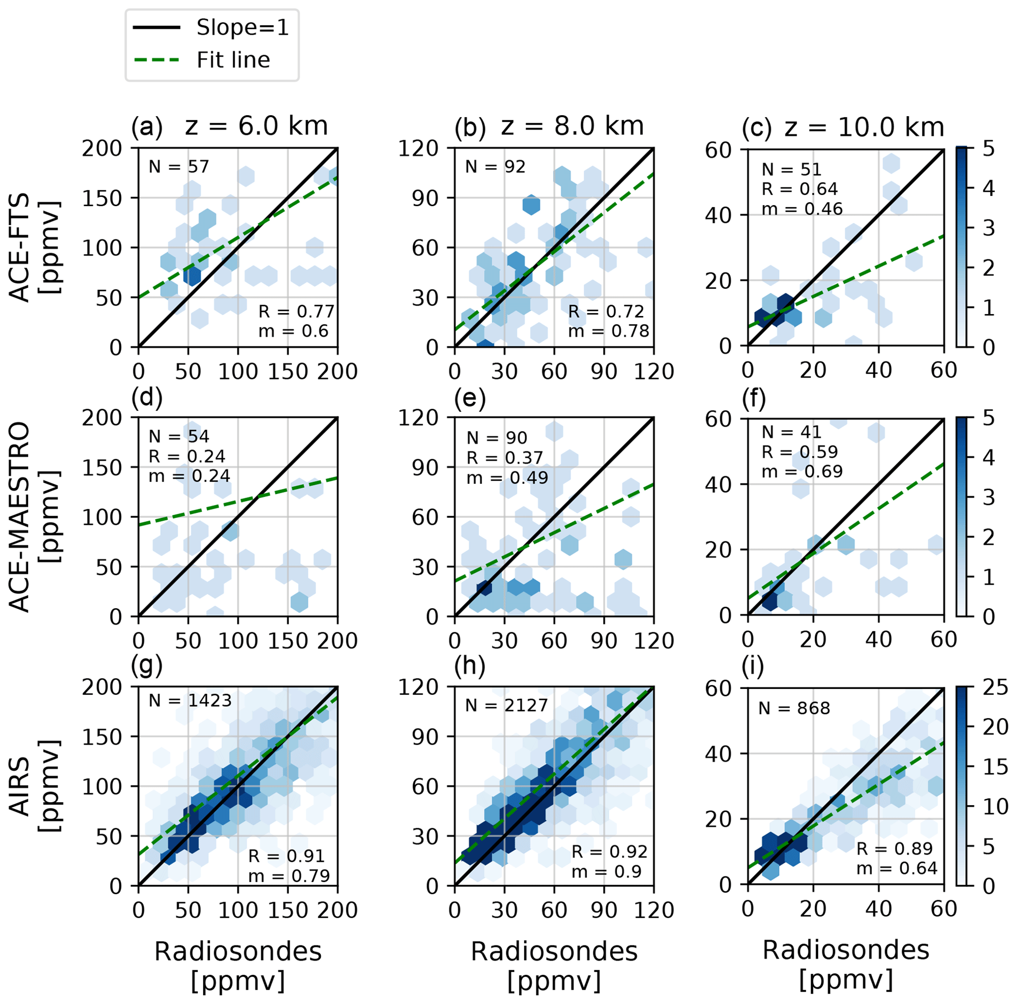
Figure 11Same as Fig. 8, but with correlation plots for the ACE-FTS, ACE-MAESTRO, and AIRS satellite measurements vs. the Eureka radiosondes.
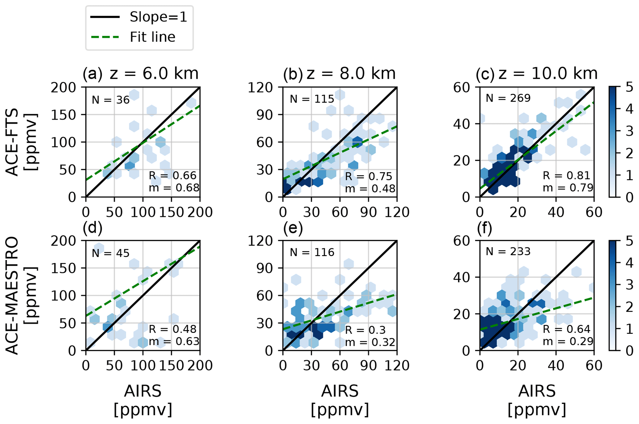
Figure 12Same as Fig. 10, but with correlation plots for the ACE-FTS and ACE-MAESTRO vs. the AIRS satellite measurements.
3.2.4 Other satellite measurements vs. ground-based references
AIRS
Close agreement was observed between 3189 coincident AIRS and 125HR measurements and between 2489 coincident AIRS and radiosonde profiles. AIRS profiles agree with the 125HR within 5 % between 1 and 14 km, as shown in Fig. 6. A mean difference of ppmv ( %) was observed between AIRS and 125HR measurements at 6.4 km, where both instruments have good sensitivity. This is shown in Fig. 7b. In the mid-troposphere, agreement is within 4 %. Correlation coefficients at all altitudes are above 0.84. Correlation plots for AIRS vs. 125HR at 6.4, 8.0, and 9.8 km are shown in Fig. 8.
Mean agreement within 5 % is observed between AIRS and the radiosondes between 1 and 7 km, as shown in Fig. 9. Differences as large as 13 % are observed between 8 and 14 km. Differences at 10 km are shown in Fig. 9b, where scatter around zero is seen. In addition, the time series of differences shows a potential seasonality to the agreement, with a low (dry) bias maximum in summer. Tightening the coincidence criteria to 2 h and 25 km significantly reduces the number of matches, with 45 contributing to comparisons at 1 km and 1255 contributing to comparisons at 8 km. Results from these tighter matches show differences of less than 4 % between 2 and 7 km, with slightly larger differences at 1 km. Differences remained similar between 8 and 14 km with these stricter coincidence criteria.
MIPAS
MIPAS v5 and v7 comparisons with the PEARL 125HR show a dry bias of approximately 15 % in the upper troposphere. At 6.4 km, the lowest altitude available for comparisons with a reasonable number of coincident measurements (N=64), mean differences using MIPAS v5 were ppmv ( %). MIPAS v7 showed similar differences to v5 with respect to the 125HR at 6.4 km, i.e. ppmv ( %). The time series of differences between the 125HR and MIPAS datasets at 6.4 km is illustrated in Fig. 7c, showing large scatter. Correlation at 6.4 km was moderate (R=0.50). Between 7 and 14 km a good correlation was observed for both retrieval versions (R > 0.81). Agreement improves between 7 and 10 km. MIPAS v5 reaches a mean difference of ppmv ( %) at 9.8 km. Above 10 km, differences are small, less than 2 ppmv and 7 %.
No MIPAS measurements were coincident with radiosondes. This is in part due to the partial overlap of the datasets (September 2008 to April 2012) and also because MIPAS only had Eureka coincidences during midday and midnight, limiting matches within 3 h of radiosonde launches.
If AIRS is used as a reference, MIPAS v5 and v7 have hundreds or thousands of matches for comparison at each altitude level. The results show that MIPAS has a dry bias relative to AIRS of approximately 15 % between 6 and 10 km, comparable to the 125HR results.
MLS
Relative to the 125HR, an MLS dry bias is observed in the UTLMS, where mean differences range from ppmv ( %) at 8.8 km to ppmv ( ppbv; %) at 13.6 km. This can be seen in Fig. 6. At 9.8 km, mean differences between 2443 coincidences were ppmv ( %); at 12.0 km, mean differences between 2445 coincidences were ppmv ( %).
MLS comparisons with the radiosondes have overlap only between 9 and 13 km; comparisons are shown in Fig. 9. At altitudes between 9 and 12 km the matched measurements are highly correlated, with R values between 0.83 and 0.92. Comparisons between MLS and radiosondes showed a dry bias at altitudes between 8 and 12 km. At 10 km, MLS had 447 coincidences with radiosonde measurements, with a mean differences of ppmv ( %). The time series of differences between MLS and the radiosondes at 10 km is shown in Fig. 10c.
SCIAMACHY
SCIAMACHY could be compared only with the 125HR, as its measurements did not have coincidences with the radiosonde dataset used in this study; 201 SCIAMACHY v3.01 and 1506 SCIAMACHY v4.2 profiles had coincidences with the 125HR. However, these are limited to altitudes above 10 km. Profile comparison results are shown in Fig. 6. For both retrieval versions, a small dry bias is seen with respect to the 125HR at 10.8 and 12.0 km, i.e. 5 % for v3.01 and 10 % for v4.2. At 13.6 km, mean differences were about 1 %.
TES
TES shows moderate agreement with the PEARL 125HR, but TES had only a single coincidence with the Eureka radiosonde dataset. The latter is largely because TES had no coincidences with Eureka after September 2008, except for a few during mid-July 2011 (Fig. 1). As shown in Fig. 6, 361 TES measurements showed a dry bias relative to the 125HR of approximately 10 % in the lower troposphere, a small dry bias (e.g. −1 % at 3.0 km) to a small wet bias in the mid-troposphere (e.g. 3.7 % at 3.6 km), and a wet bias (e.g. 20 %–25 %) in the UTLS. The time series of differences at 6.4 km is shown in Fig. 7c, where large scatter is seen, e.g. σ=75.1 %.
3.3 Summary of profile comparisons
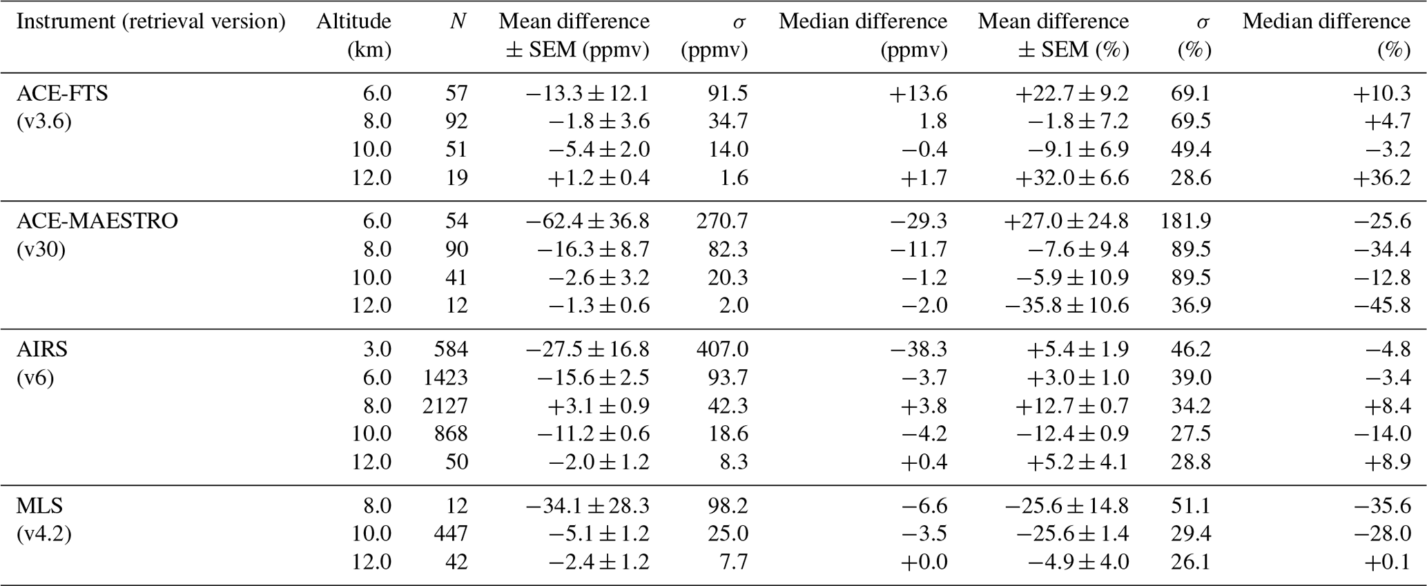
A summary of comparisons between the satellites and the PEARL 125HR is presented in Table 2. Table 3 provides a summary of the comparisons between the satellites and the Eureka radiosondes. In addition to the number of measurements, means, standard deviations, and SEMs at each altitude, these tables also include the medians of the differences. If the distance criterion was reduced to 350 km, similar differences were observed, but with a much smaller number of coincident measurements in some cases. There is no apparent temporal trend in the differences between satellite datasets and the Eureka-based reference measurements.
Table 3Summary of satellite vs. radiosonde comparison results. SEM refers to the standard error in the mean, i.e. .
In addition to the comparison results presented in Figs. 6–12, six figures are presented in the Supplement. Figure S1 shows the time series of differences for the satellite datasets and 125HR at 8 km. Figures S3 through S5 show differences between the satellite datasets and the radiosondes at 6, 8, and 12 km altitudes. Two additional figures, formatted in the same manner as Figs. 6 and 9, show profile comparison results for example days where all satellite datasets had coincident measurements with the 125HR (Fig. S6) and with the radiosondes (Fig. S7).
In some comparisons, e.g. the comparison between AIRS and the radiosondes at 12 km, the reported mean of the absolute differences and percent differences were different signs, e.g. the mean of the absolute differences was negative while the mean of the percent differences was positive. This is the result of reporting the mean of individual comparisons rather than comparing the mean profiles of each instrument. The latter would ensure that the sign is always the same in both cases. Percent differences are weighted differently than the absolute differences when the mean is calculated. Histograms were plotted for the differences between each instrument comparison at each altitude discussed in this study. These results (not shown) showed that the differences are typically distributed in a nearly Gaussian manner, justifying the use of the mean, SEM, and standard deviation to characterize the results.
This study's moderately tight temporal criterion, 3 h, aimed to minimize the impact of water vapour's variability on the observed agreement. The variability in water vapour over the 500 km distance criterion likely contributes to the differences observed between measurements. This is especially true for lower-tropospheric measurements, given the variability in surface terrain in the region around Eureka. The seasonally changing tropopause height also introduces a source of variability, particularly for altitudes between 8 and 10 km. In the summer, the TPH is often above 8 km at Eureka and is sometimes above 10 km. The TPH can be as low as 6 km. H2O abundances and variability are typically larger at altitudes below the TPH. However, no seasonal pattern in the differences, or pattern with respect to the TPH, was observed.
Measurement techniques also result in differences in the air sampled. While radiosondes measure air close to Eureka throughout their profile, the 125HR's solar-viewing geometry primarily samples air south of Eureka due to the large SZA of high-latitude measurements. Limb-sounding satellite measurement techniques used by ACE-FTS, ACE-MAESTRO, MIPAS, MLS, and SCIAMACHY yield vertical profiles by observing across long horizontal stretches of atmosphere. While this technique enables the retrieval to resolve vertical structure, this horizontal path results in profiles containing information about the atmosphere across an extended area. Thus, exact agreement between the satellite and ground-based measurements is not expected. It is worth noting that all of the instruments' measurement techniques observe the atmosphere only in cloud-free conditions, except the Eureka radiosondes.
Since ACE coincidences with Eureka are limited to periods of time when water vapour abundances are relatively similar across the region, the distance criterion is expected to have less impact on the observed agreement than if year-round measurements were compared. Typical March and July water vapour abundances in the area around Eureka are shown in Fig. 3.
Agreement between both ACE instruments and the Eureka reference measurements was closer than that observed in comparisons conducted by Carleer et al. (2008), which examined an earlier version of these datasets (e.g. ACE-FTS v2.2) and reported differences on the order of 40 % at altitudes lower than 15 km and a possible dry bias at around 10 km altitude. Sheese et al. (2017) reported an ACE-FTS negative bias ranging between 3 % and 20 % relative to MLS and MIPAS at around 14 km; however, the Sheese et al. analysis involves measurements taken over a broad range of global geographic locations and did not discuss altitudes below 13 km.
The ACE-FTS comparisons presented here show a positive (wet) bias of between 7 % and 10 % relative to the 125HR in the 8 to 14 km altitude range. Relative to the Eureka radiosondes, ACE-FTS shows very close agreement (within 4 % or 6 ppmv) in the upper troposphere (7 to 9 km). At altitudes above 10 km, a positive (wet) bias relative to the radiosondes is observed, ranging between 12 % and 32 %, although this corresponds to very small mean differences, i.e. those of about 1 ppmv. If AIRS is taken as a reference, a larger number of coincidences are found and similar results are observed, although with closer agreement around 10 km. These results indicate that ACE-FTS offers accurate H2O profiles in the Arctic UTLS region, e.g. down to 7 km.
ACE-MAESTRO profiles show a dry bias relative to the 125HR of approximately 10 % down to 7 km. Comparisons to the radiosondes also showed a dry bias, ranging from −3 % at 7 km to −21 % at 11 km. At 6 km and below, large differences between ACE-MAESTRO and the radiosonde profiles are large, as was the case in the 125HR comparison; however, in both cases there are too few coincidences for firm conclusions. Using AIRS as a reference results in hundreds of coincidences and similar results, e.g. similar magnitudes with an increasingly large difference at altitudes below 7 km.
ACE-MAESTRO shows weak correlations with the Eureka 125HR and radiosonde datasets in Figs. 8 and 11. However, this is likely due to the combination of water vapour's variability, seen in the Figs. 8 and 11 correlation plots involving AIRS and the relatively low number of coincidences found. As shown in Fig. 12, the number of coincidences and the correlations between ACE-MAESTRO and AIRS are much larger, e.g. N=233 and R=0.64 at 10 km, while the differences are similar to other comparisons, e.g. there were large differences at 6 km. In addition, the correlation and best-fit line are impacted by outlier points at low altitudes (e.g. at 6.4 km in the comparison with the 125HR) that influence the overall statistics because of the relatively small number of coincidences at those altitudes. ACE-FTS correlation plots are also affected by outliers.
For both ACE-FTS and ACE-MAESTRO, measurements at altitudes below approximately 5 km are often not possible because ACE's sun tracker is unable to lock onto the Sun reliably due to cloud effects and refraction (Boone et al., 2005). This issue may contribute to the larger differences observed at low altitudes. This is especially the case with ACE-MAESTRO, whose retrieval produces profiles extend as low as 4 km with tangent heights determined by extrapolation based on the vertical sampling above 5 km.
AIRS and TES are the only satellite instruments in this study whose measurements are performed in nadir-viewing modes and whose retrieval products reach the lower troposphere. Humidity inversions typically occur near Eureka between 500 m and 2 km in altitude. Sometimes, a major structure is seen in the water vapour profile between 2 and 4 km as well. Individual profile-to-profile comparisons with the Eureka radiosondes show that AIRS retrievals do not fully capture structure in the humidity inversion feature, explaining much of the individual profile differences at the lowest altitude levels. This is expected because the vertical resolution of AIRS is not always sufficient for resolving these vertical structures (Susskind et al., 2014). The AIRS user guide warns of occasional “strange results” in proximity to near-surface humidity inversions; however, the AIRS profiles coincident with Eureka showed no features that were oddly shaped or clearly erroneous. The magnitude of the inversion was often inaccurate, or the inversion was not seen in the AIRS profile. This could also be in part due to a geographic or temporal mismatch between the measurements.
Similarly, individual profile-to-profile comparisons with the nearest radiosonde profile show that TES profiles often capture the general shape of the lower-tropospheric humidity profiles structure; however, the smoothing operation is not sufficient for bringing the measurements into agreement. It is possible that the DOFSs of the TES retrieval are overestimated. Where radiosondes from earlier or later in the day reveal a humidity profile with a vertical structure that is less fine, agreement between TES and the 125HR was much closer.
This study compared high Arctic UTLS water vapour measurements taken by seven satellite-based instruments with measurements acquired by the Eureka radiosondes and the PEARL 125HR. The focus of the work was to assess the UTLS water vapour retrieved from ACE-FTS and ACE-MAESTRO measurements. The ACE instruments' ability to observe UTLS water vapour is a valuable contribution to global atmospheric monitoring, as its profiles extend to lower altitudes than many other satellite-based measurements, particularly those retrieved from limb-viewing observations.
ACE-FTS and ACE-MAESTRO showed good agreement with both the radiosondes and the 125HR in the UTLS. No obvious temporal trend is apparent in the differences. ACE-FTS showed a wet bias of approximately 7 % to 10 % relative to the 125HR. An ACE-FTS dry bias of 2 % to 9 % was observed relative to the radiosondes between 8 and 10 km. While agreement is observed in the upper troposphere, the observed agreement did not reach the 5 % accuracy goal set by GCOS. ACE-MAESTRO profiles at altitudes below 7 km had large differences relative to both the radiosondes and the 125HR; between 8 and 10 km, a dry bias between 6 % and 18 % is observed relative to both the radiosondes and the 125HR. Nonetheless, ACE water vapour measurements showed closer agreement overall with the Eureka reference measurements in the UTLS than the other satellite datasets examined in this study, with the exception of AIRS.
AIRS water vapour profiles showed close agreement with both the 125HR and radiosonde measurements, i.e. within the 5 % GCOS target. The observed accuracy of the AIRS measurements suggests that they can be used for analysis of humidity conditions near Eureka. Given the high density and frequency of AIRS measurements, it would be worthwhile to use AIRS measurements to create climatologies of water vapour conditions near the site and also to examine patterns of water vapour abundances in the region. AIRS data may also be useful for validation studies in cases where radiosonde and 125HR measurements do not offer sufficient numbers of coincident measurements. In addition, global UTLS comparisons between AIRS and ACE water vapour measurements could also be examined to better understand the accuracy of the ACE-FTS and ACE-MAESTRO water vapour datasets.
MIPAS and SCIAMACHY comparisons at altitudes where the data are recommended (i.e. above 10 km) showed agreement within 6 % of the 125HR. Coincidences with the radiosondes were not available. At UTLS altitudes where the MIPAS data are not recommended for use but are included in the publicly available data product, large differences and variability were observed. This supports the recommendation of limiting the use of MIPAS v5 and v7 water vapour profiles to 12 km and above. MIPAS v5 and v7 and SCIAMACHY v3.01 and v4.2 comparison results were very similar.
MLS comparisons with the radiosondes and 125HR between 8 and 12 km showed a dry bias. This aligns with UTLS-region MLS dry biases observed by Hurst et al. (2016) and Vömel et al. (2007b) using FPH measurements.
Future work with these satellite datasets could involve an analysis of water vapour abundances in the UTLS across the Arctic, e.g. using ACE measurements. Moreover, the density of measurements and close agreement between AIRS and the Eureka GRUAN-processed radiosonde dataset motivate the use of the AIRS dataset in investigating water vapour abundances across the Arctic throughout the troposphere.
FPH water vapour measurements at Eureka would enhance the ongoing satellite validation work there and enable a valuable reference for PEARL water vapour measurements. FPH measurements would offer improved accuracy as well as better coverage throughout UTLS altitudes relative to the radiosondes and 125HR. FPH measurements have been used for the validation of other missions, such as MLS (Hurst et al., 2016) and MIPAS (Stiller et al., 2012; using the MOHAVE measurements). Adding FPH measurements would be a useful next step for the comparison and validation of water vapour profiles at Eureka.
The satellite datasets used in this study are available for download through their respective websites. All require registration except TES and MUSICA. ACE-FTS and ACE-MAESTRO data can be accessed at http://www.ace.uwaterloo.ca/data.php (ACE, 2019). AIRS data can be accessed at https://airs.jpl.nasa.gov/data/get_data (AIRS, 2019), MIPAS (IMK retrieval) data at https://www.imk-asf.kit.edu/english/308.php\#org0f1a3a1 (MIPAS, 2019), MLS data at https://mls.jpl.nasa.gov/ (MLS, 2019), SCIAMACHY data at http://www.iup.uni-bremen.de/scia-arc/ (SCIAMACHY, 2019), and TES data at https://tes.jpl.nasa.gov/data/ (TES, 2019). The PEARL 125HR water vapour data are available through the online MUSICA repository at ftp://ftp.cpc.ncep.noaa.gov/ndacc/MUSICA/ (MUSICA, 2019).
However, the dataset used in this study has relaxed the usual solar zenith angle criterion to expand available measurements to the high-latitude site of Eureka. Please contact Dan Weaver (dweaver@atmosp.physics.utoronto.ca) regarding access to this dataset.
Radiosonde data used in this study are owned by Environment and Climate Change Canada and are not currently available online. Please contact Dan Weaver (dweaver@atmosp.physics.utoronto.ca) regarding access to this dataset.
The supplement related to this article is available online at: https://doi.org/10.5194/amt-12-4039-2019-supplement.
DW led the study, performed 125HR measurements, gathered the datasets, calculated the comparisons between the datasets, created the figures and tables, and wrote the paper. KS advised and guided the work and provided significant editing, advice, and comments. KAW contributed insight into the ACE-FTS dataset as well as helpful comments on the paper. CS contributed the ACE-MAESTRO water vapour dataset as well as helpful comments on the paper and discussions about the meteorological conditions at Eureka. MS performed the 125HR retrievals following the MUSICA technique and offered detailed comments. HV offered insight into the radiosonde data and their use. MS processed the raw Eureka radiosonde measurement files according to the GRUAN technique. CTM contributed insight and comments regarding the ACE-MAESTRO measurement comparisons.
JPB proposed and leads the SCIAMACHY project; in this context, initiating the concept used for the limb H2O profile algorithm, he contributed to and advised on its evolution, as used in this study. AR leads the limb retrieval group which has developed key parts of the H2O retrieval algorithm. KW is an expert on limb remote sensing, having led the development the v3.1 and v.4 H2O limb product, validated the data products, and initiated and coordinated the IUP contribution to this study.
WGR contributed expertise about the MLS dataset. EF offered helpful comments on the paper and insight regarding the AIRS dataset. GS offered helpful comments about the paper and insight on the MIPAS dataset.
The authors declare that they have no conflict of interest.
This article is part of the special issue “Water vapour in the upper troposphere and middle atmosphere: a WCRP/SPARC satellite data quality assessment including biases, variability, and drifts (ACP/AMT/ESSD inter-journal SI)”. It is not associated with a conference.
This work was primarily funded by the National Sciences and Engineering Research Council (NSERC) through the Probing the Atmosphere of the High Arctic (PAHA) project. Spring visits to PEARL were made as part of the Canadian Arctic ACE/OSIRIS Validation Campaigns funded by the Canadian Space Agency (CSA), with additional support from Environment and Climate Change Canada (ECCC), NSERC, and the Northern Scientific Training Program.
CANDAC–PEARL funding partners are the Arctic Research Infrastructure Fund, Atlantic Innovation Fund and Nova Scotia Research Innovation Trust, Canadian Foundation for Climate and Atmospheric Sciences, Canada Foundation for Innovation, CSA, ECCC, Government of Canada International Polar Year, NSERC, Ontario Innovation Trust, Ontario Research Fund, Indigenous and Northern Affairs Canada, and the Polar Continental Shelf Program. This work also received funding from the NSERC CREATE Training Program in Arctic Atmospheric Science and the CSA-supported Canadian FTIR Observing Network (CAFTON) and Arctic Validation and Training for Atmospheric Research in Space (AVATARS) projects.
The authors would like to thank PEARL principal investigator James Drummond, PEARL site manager Pierre Fogal, and the CANDAC operators for logistical and operational support at Eureka; ECCC for providing the radiosonde data; Rodica Lindenmaier, Rebecca Batchelor, and Joseph Mendonca for 125HR measurements; and CANDAC Data Manager Yan Tsehtik.
The authors wish to thank the staff at ECCC's Eureka Weather Station for logistical and on-site support.
MUSICA has been funded by the European Research Council under the European Community's Seventh Framework Programme (FP7/2007-2013) – ERC grant agreement number 256961.
The Atmospheric Chemistry Experiment is a Canadian-led satellite mission mainly supported by the CSA.
We thank the satellite data retrieval and validation teams for the ACE, AIRS, MIPAS, MLS, SCIAMACHY, and TES missions as well as their funding agencies.
Part of the research was carried out at the Jet Propulsion Laboratory, California Institute of Technology, under a contract with the National Aeronautics and Space Administration.
The SCIAMACHY limb water vapour datasets v3.01 and v4.2 are a result of the DFG (German Research Council) Research Unit “Stratospheric Change and its Role for Climate Prediction” (SHARP) and the ESA SPIN (ESA SPARC Initiative) and SQWG (SCIAMACHY Quality Working Group) projects and were calculated using resources of the German HLRN (High-Performance Computer Center North).
Figures 3, 5, 8, 11, and 12 were produced using Python and the Matplotlib and NumPy packages. The authors would like to thank those development communities.
This research has been supported by the Natural Sciences and Engineering Research Council of Canada (grant no. RGPCC-433842-2012), the Canadian Space Agency (grant no. 14SUSCISAT), and the Seventh Framework Programme (MUSICA – grant no. 256961).
This paper was edited by Andreas Hofzumahaus and reviewed by four anonymous referees.
ACE: SCISAT Data, available at: http://www.ace.uwaterloo.ca/data.php, last access: 16 July 2019.
Adams, C., Strong, K., Batchelor, R. L., Bernath, P. F., Brohede, S., Boone, C., Degenstein, D., Daffer, W. H., Drummond, J. R., Fogal, P. F., Farahani, E., Fayt, C., Fraser, A., Goutail, F., Hendrick, F., Kolonjari, F., Lindenmaier, R., Manney, G., McElroy, C. T., McLinden, C. A., Mendonca, J., Park, J.-H., Pavlovic, B., Pazmino, A., Roth, C., Savastiouk, V., Walker, K. A., Weaver, D., and Zhao, X.: Validation of ACE and OSIRIS ozone and NO2 measurements using ground-based instruments at 80∘ N, Atmos. Meas. Tech., 5, 927–953, https://doi.org/10.5194/amt-5-927-2012, 2012.
AIRS: Get AIRS Data, available at: https://airs.jpl.nasa.gov/data/get_data, last access: 16 July 2019.
Barthlott, S., Schneider, M., Hase, F., Blumenstock, T., Kiel, M., Dubravica, D., García, O. E., Sepúlveda, E., Mengistu Tsidu, G., Takele Kenea, S., Grutter, M., Plaza-Medina, E. F., Stremme, W., Strong, K., Weaver, D., Palm, M., Warneke, T., Notholt, J., Mahieu, E., Servais, C., Jones, N., Griffith, D. W. T., Smale, D., and Robinson, J.: Tropospheric water vapour isotopologue data (, H)218O, and HD16O) as obtained from NDACC/FTIR solar absorption spectra, Earth Syst. Sci. Data, 9, 15–29, https://doi.org/10.5194/essd-9-15-2017, 2017.
Batchelor, R., Strong, K., Lindenmaier, R., Mittermeier, R., Fast, H., Drummond, J. R., and Fogal, P.: A New Bruker IFS 125HR FTIR Spectrometer for the Polar Environment Atmospheric Research Laboratory at Eureka, Nunavut, Canada: Measurements and Comparison with the Existing Bomem DA8 Spectrometer, J. Atmos. Ocean. Tech., 26, 1328–1340, 2009.
Beer, R., Glavich, T. A., and Rider, D. M.: Tropospheric emission spectrometer for the Earth Observing System's Aura Satellite, Appl. Opt., 40, 2356–2367, 2001.
Bernath, P., McElroy, C., Abrams, M., Boone, C., Butler, M. C.-P., Camy-Peyret, C., Carleer, M., Clerbaux, M., Coheur, P.F., Colin, R., DeCola, P., DeMaziere, M., Drummond, J. R., Dufour, D., Evans, W. F. J., Fast, H., Fussen, D., Gilbert, K., Jennings, D. E., Llewellyn, E. J., Lowe, R. P., Mahieu, E., McConnell, J. C., McHugh, M., McLeod, S. D., Michaud, R., Midwinter, C., Nassar, R., Nichitiu, F., Nowlan, C., Rinsland, C. P., Rochon, Y. J., Rowlands, N., Semeniuk, K., Simon, P., Skelton, R., Sloan, J. J., Soucy, M.-A., Strong, K., Tremblay, P., Turnbull, D., Walker, K. A., Walker, I., Wardle, D. A., Wehrle, V., Zander, R., and Zou, J.: Atmospheric Chemistry Experiment (ACE): Mission overview, Geophys. Res. Lett., 32, L15S01, https://doi.org/10.1029/2005GL022386, 2005.
Bernath, P. F.: The Atmospheric Chemistry Experiment (ACE), J. Quant. Spectrosc. Ra., 186, 3–16, https://doi.org/10.1016/j.jqsrt.2016.04.006, 2017.
Boone, C. D., Nassar, R., Walker, K. A., Rochon, Y., McLeod, S. D., Rinsland, C. P., and Bernath, P. F.: Retrievals for the Atmospheric Chemistry Experiment Fourier-transform spectrometer, Appl. Opt., 44, 7218–7231, https://doi.org/10.1364/AO.44.007218, 2005.
Boone, C. D., Walker, K. A., and Bernath, P. F.: Version 3 Retrievals for the Atmospheric Chemistry Experiment Fourier Transform Spectrometer (ACE-FTS) in The Atmospheric Chemistry Experiment ACE at 10: A Solar Occultation Anthology, edited by: Bernath, P. F., A. Deepak Publishing, Hampton, Virginia, 2013.
Bovensmann, H., Burrows, J. P., Buchwitz, M., Frerick, J., Noël, S., Rozanov, V. V., Chance, K. V., and Goede, A. P.: SCIAMACHY: Mission Objectives and Measurement Modes, J. Atmos. Sci., 56, 127–150, https://doi.org/10.1175/1520-0469(1999)056<0127:SMOAMM>2.0.CO;2, 1999.
Bowman, K. W., Rodgers, C. D., Sund-Kulawik, S., Worden, J., Sarkissian, E., Osterman, G., Steck, T., Lou, M., Eldering, A., Shepherd, M., Worden, H., Lampel, M., Clough, S., Brown, P., Rinsland, C., Gunson, M., and Beer, R.: Tropospheric Emission Spectrometer: Retrieval Method and Error Analysis. IEEE T. Geosci. Remote, 44, 1297–1307, 2006.
Buchholz, R. R., Deeter, M. N., Worden, H. M., Gille, J., Edwards, D. P., Hannigan, J. W., Jones, N. B., Paton-Walsh, C., Griffith, D. W. T., Smale, D., Robinson, J., Strong, K., Conway, S., Sussmann, R., Hase, F., Blumenstock, T., Mahieu, E., and Langerock, B.: Validation of MOPITT carbon monoxide using ground-based Fourier transform infrared spectrometer data from NDACC, Atmos. Meas. Tech., 10, 1927–1956, https://doi.org/10.5194/amt-10-1927-2017, 2017.
Carleer, M. R., Boone, C. D., Walker, K. A., Bernath, P. F., Strong, K., Sica, R. J., Randall, C. E., Vömel, H., Kar, J., Höpfner, M., Milz, M., von Clarmann, T., Kivi, R., Valverde-Canossa, J., Sioris, C. E., Izawa, M. R. M., Dupuy, E., McElroy, C. T., Drummond, J. R., Nowlan, C. R., Zou, J., Nichitiu, F., Lossow, S., Urban, J., Murtagh, D., and Dufour, D. G.: Validation of water vapour profiles from the Atmospheric Chemistry Experiment (ACE), Atmos. Chem. Phys. Discuss., 8, 4499–4559, https://doi.org/10.5194/acpd-8-4499-2008, 2008.
Chahine, M. T.: GEWEX: The Global Energy and Water Cycle Experiment, EOS, 73, 13–14, https://doi.org/10.1029/91EO00007, 1992.
Chahine, M. T., Pagano, T. S., Aumann, H. H., Atlas, R., Barnet, C., Blaisdell, J., Chen, L., Divakarla, M., Fetzer, E.J., Goldberg, M., Gauthier, C., Granger, S., Hannon, S., Irion, F.W., Kakar, R., Kalnay, E., Lambrigtsen, B.H., Lee, S., Le Marshall, J., McMillan, W. W., McMillin, L., Olsen, E. T., Revercomb, H., Rosenkranz, P., Smith, W.L., Staelin, D., Strow, L.L., Susskind, J., Tobin, D., Wolf, W., and Zhou, L.: AIRS Improving Weather Forecasting and Providing New Data on Greenhouse Gases, B. Am. Meteorol. Soc., 87, 911–926, https://doi.org/10.1175/BAMS-87-7-911, 2006.
Dessler, A. E., Zhang, Z., and Yang, P.: Water vapor climate feedback inferred from climate fluctuations, 2003–2008, Geophys. Res. Lett., 35, L20704, https://doi.org/10.1029/2008GL035333, 2008.
Dessler, A. E., Schoeberl, M. R., Wang, T., Davis, S. M., and Rosenlof, K. H.: Stratospheric water vapor feedback, P. Natl. Acad. Sci. USA, 110, 18087–18091, https://doi.org/10.1073/pnas.1310344110, 2013.
Dirksen, R. J., Sommer, M., Immler, F. J., Hurst, D. F., Kivi, R., and Vömel, H.: Reference quality upper-air measurements: GRUAN data processing for the Vaisala RS92 radiosonde, Atmos. Meas. Tech., 7, 4463–4490, https://doi.org/10.5194/amt-7-4463-2014, 2014.
Durre, I., Vose, R. S., and Wuertz, D. B.: Overview of the Integrated Global Radiosonde Archive, J. Climate, 19, 53–68, https://doi.org/10.1175/JCLI3594.1, 2006.
Fischer, H., Birk, M., Blom, C., Carli, B., Carlotti, M., von Clarmann, T., Delbouille, L., Dudhia, A., Ehhalt, D., Endemann, M., Flaud, J. M., Gessner, R., Kleinert, A., Koopman, R., Langen, J., López-Puertas, M., Mosner, P., Nett, H., Oelhaf, H., Perron, G., Remedios, J., Ridolfi, M., Stiller, G., and Zander, R.: MIPAS: an instrument for atmospheric and climate research, Atmos. Chem. Phys., 8, 2151–2188, https://doi.org/10.5194/acp-8-2151-2008, 2008.
Fogal, P., LeBlanc, L. M., and Drummond, J.: The Polar Environment Atmospheric Research Laboratory (PEARL): Sounding the Atmosphere at 80∘ North, Arctic, 66, 377–386, 2013.
Fraser, A., Adams, C., Drummond, J. R., Goutail, F., Manney, G., and Strong, K.: The Polar Environment Atmospheric Research Laboratory UV-visible ground-based spectrometer: First measurements of O3, NO2, BrO, and OClO columns, J. Quant. Spectrosc. Ra., 110, 986–1004, https://doi.org/10.1016/j.jqsrt.2009.02.034, 2008.
Global Climate Observing System (GCOS): The Global Observing System for Climate: Implementation Needs. GCOS-200, available at: https://public.wmo.int/en/programmes/global-climate-observing-system (last access: 14 June 2018), 2016.
Griffin, D., Walker, K. A., Conway, S., Kolonjari, F., Strong, K., Batchelor, R., Boone, C. D., Dan, L., Drummond, J. R., Fogal, P. F., Fu, D., Lindenmaier, R., Manney, G. L., and Weaver, D.: Multi-year comparisons of ground-based and space-borne Fourier transform spectrometers in the high Arctic between 2006 and 2013, Atmos. Meas. Tech., 10, 3273–3294, https://doi.org/10.5194/amt-10-3273-2017, 2017.
Hase, F., Hannigan, J. W., Coffey, M. T., Goldman, A., Höpfner, M., Jones, N. B., Rinsland, C. P., and Wood, S. W.: Intercomparison of retrieval codes used for the analysis of high-resolution, ground-based FTIR measurements, J. Quant. Spectrosc. Ra., 87, 25–52, 2004.
Hegglin, M. I., Tegtmeier, S., Anderson, J., Froidevaux, L., Fuller, R., Funke, B., Jones, A., Lingenfelser, G., Lumpe, J., Pendlebury, D., Remsberg, E., Rozanov, A., Toohey, M., Urban, J., von Clarmann, T., Walker, K. A., Wang, R., and Weigel, K.: SPARC Data Initiative: Comparison of water vapor climatologies from international satellite limb sounders. J. Geophys. Res.-Atmos., 118, 11824–11846, https://doi.org/10.1002/jgrd.50752, 2013.
Herman, R. and Kulawik, S. (Eds.): Earth Observing System (EOS) Tropospheric Emission Spectrometer (TES) Data Validation Report (Version F07_10 data). JPL Internal Report D-33192, available at: https://eosweb.larc.nasa.gov/sites/default/files/project/tes/readme/TES_Validation_Report_v6.pdf, last access: 5 November 2013.
Herman, R. and Osterman, G. (Eds.): Earth Observing System (EOS) Tropospheric Emission Spectrometer (TES) Level 2 (L2) Data User's Guide (Up to & including Version 6 data), Version 6.0, JPL Internal Report D-38042, available at: https://tes.jpl.nasa.gov/documents/, last access: 20 June 2014.
Hurst, D. F., Lambert, A., Read, W. G., Davis, S. M., Rosenlof, K. H., Hall, E. G., Jordan, A. F., and Oltmans, S. J.: Validation of Aura Microwave Limb Sounder stratospheric water vapor measurements by the NOAA frost point hygrometer. J. Geophys. Res.-Atmos., 119, 1612–1625, https://doi.org/10.1002/2013JD020757, 2014.
Hurst, D. F., Read, W. G., Vömel, H., Selkirk, H. B., Rosenlof, K. H., Davis, S. M., Hall, E. G., Jordan, A. F., and Oltmans, S. J.: Recent divergences in stratospheric water vapor measurements by frost point hygrometers and the Aura Microwave Limb Sounder, Atmos. Meas. Tech., 9, 4447–4457, https://doi.org/10.5194/amt-9-4447-2016, 2016.
Hyland, R. W. and Wexler, A.: Formulations for the Thermodynamic Properties of the Saturated Phases of H2O from 173.15 K to 473.15 K, ASHRAE, 2793, 500–511, 1983.
Khosrawi, F., Lossow, S., Stiller, G. P., Rosenlof, K. H., Urban, J., Burrows, J. P., Damadeo, R. P., Eriksson, P., García-Comas, M., Gille, J. C., Kasai, Y., Kiefer, M., Nedoluha, G. E., Noël, S., Raspollini, P., Read, W. G., Rozanov, A., Sioris, C. E., Walker, K. A., and Weigel, K.: The SPARC water vapour assessment II: comparison of stratospheric and lower mesospheric water vapour time series observed from satellites, Atmos. Meas. Tech., 11, 4435–4463, https://doi.org/10.5194/amt-11-4435-2018, 2018.
Lesins, G., Duck, T. J., and Drummond, J. R.: Climate Trends at Eureka in the Canadian High Arctic, Atmos. Ocean, 48, 59–80, 2010.
Livesey, N. J., Read, W. G., Wagner, P. A., Froidevaux, L., Lambert, A., Manney, G. L., Millán Valle, L. F., Pumphrey, H. C., Santee, M. L., Schwartz, M. J., Wang, S., Fuller, R. A., Jarnot, R. F., and Knosp, B. W.: Aura Microwave Limb Sounder Version 4.2x Level 2 data quality and description document, JPL D-333509 Rev. B, Version 4.2x-2.0, May 9, 2016, available at: https://mls.jpl.nasa.gov/data/datadocs.php (last access: 14 June 2018), 2016.
McElroy, C. T., Nowlan, C. R., Drummond, J. R., Bernath, P. F., Barton, D. V., Dufour, D. G., Midwinter, C., Hall, R. B., Ogyu, A., Ullberg, A., Wardle, D. I., Kar, J., Zou, J., Nichitiu, F., Boone, C. D., Walker, K. A., and Rowlands, N.: The ACE-MAESTRO instrument on SCISAT: description, performance, and preliminary results, Appl. Optics, 46, 4341–4356, 2007.
Miloshevich, L. M., Vömel, H., Whiteman, D. N., Lesht, B. M., Schmidlin, F. J., and Russo, F.: Absolute accuracy of water vapor measurements from six operational radiosonde types launched during AWEX-G and implications for AIRS validation. J. Geophys. Res., 111, D09S10, https://doi.org/10.1029/2005JD006083, 2006.
Miloshevich, L., Vömel, H., Whiteman, D., and Leblanc, T.: Accuracy assessment and correction of Vaisala RS92 radiosonde water vapor measurements. J. Geophys. Res., 114, D11305, https://doi.org/10.1029/2008JD011565, 2009.
MIPAS: Access to IMK/IAA generated MIPAS/Envisat data, available at: https://www.imk-asf.kit.edu/english/308.php#org0f1a3a1, last access: 16 July 2019.
MLS: MLS Data, available at: https://mls.jpl.nasa.gov, last access: 16 July 2019.
Müller, R., Kunz, A., Hurst, D. F., Rolf, C., Krämer, M., and Riese, M.: The need for accurate long-term measurements of water vapor in the upper troposphere and lower stratosphere with global coverage, Earth's Future, 4, 25–32, https://doi.org/10.1002/2015EF000321, 2015.
MUSICA: MUSICA/eureka, available at: ftp://ftp.cpc.ncep.noaa.gov/ndacc/MUSICA/, last access: 16 July 2019.
Olsen, E. T., Fetzer, E., Hulley, G., Kalmus, P., Manning, E., and Wong, S.: AIRS/AMSU/HSB Version 6 Level 2 product user guide, Jet Propulsion Laboratory, Version 1.6, available at: https://airs.jpl.nasa.gov/resources/guides (last access: 14 June 2018), 2017.
Parkinson, C. L.: Aqua: An earth-observing satellite mission to examine water and other climate variables, IEEE T. Geosci. Remote, 41, 173–183, https://doi.org/10.1109/TGRS.2002.808319, 2003.
Pierce, D. W., Barnett, T. P., Fetzer, E. J., and Gleckler, P.J.: Three-dimensional tropospheric water vapor in coupled climate models compared with observations from the AIRS satellite system, Geophys. Res. Lett., 33, L21701, https://doi.org/10.1029/2006GL027060, 2006.
Riese, M., Ploeger, F., Rap, A., Vogel, B., Konopka, P., Dameris, M., and Forster, P.: Impact of uncertainties in atmospheric mixing on simulated UTLS composition and related radiative effects, J. Geophys. Res., 117, D16305, https://doi.org/10.1029/2012JD017751, 2012.
Rodgers, C. and Connor, B.: Intercomparison of remote sounding instruments, J. Geophys. Res., 108, 4116, https://doi.org/10.1029/2002JD002299, 2003.
Rodgers, C. D.: Inverse Methods for Atmospheric Sounding: Theory and Practice, World Scientific Publishing Co., Hackensack, N.J., 2000.
Schneider, M., Barthlott, S., Hase, F., González, Y., Yoshimura, K., García, O. E., Sepúlveda, E., Gomez-Pelaez, A., Gisi, M., Kohlhepp, R., Dohe, S., Blumenstock, T., Wiegele, A., Christner, E., Strong, K., Weaver, D., Palm, M., Deutscher, N. M., Warneke, T., Notholt, J., Lejeune, B., Demoulin, P., Jones, N., Griffith, D. W. T., Smale, D., and Robinson, J.: Ground-based remote sensing of tropospheric water vapour isotopologues within the project MUSICA, Atmos. Meas. Tech., 5, 3007–3027, https://doi.org/10.5194/amt-5-3007-2012, 2012.
Schneider, M., Wiegele, A., Barthlott, S., González, Y., Christner, E., Dyroff, C., García, O. E., Hase, F., Blumenstock, T., Sepúlveda, E., Mengistu Tsidu, G., Takele Kenea, S., Rodríguez, S., and Andrey, J.: Accomplishments of the MUSICA project to provide accurate, long-term, global and high-resolution observations of tropospheric {H2O, δD} pairs – a review, Atmos. Meas. Tech., 9, 2845–2875, https://doi.org/10.5194/amt-9-2845-2016, 2016.
SCIAMACHY: ENVISAT SCIAMACHY value added data archive at IUP/IFE Bremen, available at: http://www.iup.uni-bremen.de/scia-arc/, last access: 16 July 2019.
Schröder, M., Lockhoff, M., Shi, L., August, T., Bennartz, R., Borbas, E., Brogniez, H., Calbet, X., Crewell, S., Eikenberg, S., Fell, F., Forsythe, J., Gambacorta, A., Graw, K., Ho, S.-P., Höschen, H., Kinzel, J., Kursinski, E. R., Reale, A., Roman, J., Scott, N., Steinke, S., Sun, B., Trent, T., Walther, A., Willen, U., and Yang, Q.: GEWEX water vapor assessment (G-VAP). WCRP Report 16/2017, World Climate Research Programme (WCRP): Geneva, Switzerland, 216 pp., 2017.
Sheese, P. E., Boone, C. D., and Walker, K. A.: Detecting physically unrealistic outliers in ACE-FTS atmospheric measurements, Atmos. Meas. Tech., 8, 741–750, https://doi.org/10.5194/amt-8-741-2015, 2015.
Sheese, P. E., Walker, K. A., Boone, C. D., Bernath, P. F., Froidevaux, L., Funke, B., Raspollini, P., and von Clarmann, T.: ACE-FTS ozone, water vapour, nitrous oxide, nitric acid, and carbon monoxide profile comparisons with MIPAS and MLS, J. Quant. Spectrosc. Ra., 186, 63–80, https://doi.org/10.1016/j.jqsrt.2016.06.026, 2017.
Shephard, M. W., Herman, R. L., Fisher, B., M., Cady-Pereira, K. E., Clough, S. A., Payne, V. H., Whiteman, D. N., Comer, J. P., Vömel, H., Miloshevich, L. M., Forno, R., Adam, M., Osterman, G. B., Eldering, A., Worden, J. R., Brown, L. R., Worden, H. M., Kulawik, S. S., Rider, D. M., Goldman, A., Beer, R., Bowman, K. W., Rodgers, C., Luo, M., Rinsland, C. P., Lampel, M., and Gunson, M. R.: Comparison of Tropospheric Emission Spectrometer nadir water vapor retrievals with in situ measurements, J. Geophys. Res., 113, D15S24, https://doi.org/10.1029/2007JD008822, 2008.
Sioris, C. E., Zou, J., McElroy, C. T., McLinden, C. A., and Vömel, H.: High vertical resolution water vapour profiles in the upper troposphere and lower stratosphere retrieved from MAESTRO solar occultation spectra, Adv. Space Res., 46, 642–650, 2010.
Sioris, C. E., Zou, J., Plummer, D. A., Boone, C. D., McElroy, C. T., Sheese, P. E., Moeini, O., and Bernath, P. F.: Upper tropospheric water vapour variability at high latitudes – Part 1: Influence of the annular modes, Atmos. Chem. Phys., 16, 3265–3278, https://doi.org/10.5194/acp-16-3265-2016, 2016.
Soden, B. J., Held, I. M., Colman, R., Shell, K. M., Kiehl, J. T., and Shields, C. A.: Quantifying climate feedbacks using radiative kernels, J. Climate, 21, 3504–3520, https://doi.org/10.1175/2007JCLI2110.1, 2008.
Solomon, S., Rosenlof, K. H., Portmann, R. W., Daniel, J. S., Davis, S. M., Sanford, T. J., and Plattner, G.-K.: Contributions of Stratospheric Water Vapor to Decadal Changes in the Rate of Global Warming, Science, 327, 1219–1223, https://doi.org/10.1126/science.1182488, 2010.
Stiller, G. P., Kiefer, M., Eckert, E., von Clarmann, T., Kellmann, S., García-Comas, M., Funke, B., Leblanc, T., Fetzer, E., Froidevaux, L., Gomez, M., Hall, E., Hurst, D., Jordan, A., Kämpfer, N., Lambert, A., McDermid, I. S., McGee, T., Miloshevich, L., Nedoluha, G., Read, W., Schneider, M., Schwartz, M., Straub, C., Toon, G., Twigg, L. W., Walker, K., and Whiteman, D. N.: Validation of MIPAS IMK/IAA temperature, water vapor, and ozone profiles with MOHAVE-2009 campaign measurements, Atmos. Meas. Tech., 5, 289-320, https://doi.org/10.5194/amt-5-289-2012, 2012.
Susskind, J., Barnet, C. D., and Blaisdell, J. M.: Retrieval of atmospheric and surface parameters from AIRS/AMSU/HSB data in the presence of clouds. IEEE T. Geosci. Remote, 41, 390–409, https://doi.org/10.1109/TGRS.2002.808236, 2003.
Susskind, J., Blaisdell, J. M., and Iredell, L.: Improved methodology for surface and atmospheric soundings, error estimates, and quality control procedures: the atmospheric infrared sounder science team version-6 retrieval algorithm, J. Appl. Rem. Sens., 8, https://doi.org/10.1117/1.JRS.8.084994, 2014.
TES: Get Data, available at: https://tes.jpl.nasa.gov/data/, last access: 16 July 2019.
Vömel, H., Selkirk, H., Miloshevich, L., Valverde-Canossa, J., Valdes, J., Kyrö, E., Kivi, R., Stolz, W., Peng, G., and Diaz, J.: Radiation dry bias of the Vaisala RS92 humidity sensor, J. Atmos. Ocean. Tech., 24, 953–963, 2007a.
Vömel, H., Barnes, J. E., Forno, R. N., Fujiwara, M., Hasebe, F., Iwasaki, S., Kivi, R., Komala, N., Kyrö, E., Leblanc, T., Morel, B., Ogino, S.-Y., Read, W. G., Ryan, S. C., Saraspriya, S., Selkirk, H., Shiotani, M., Canossa, J. V., and Whiteman, D., N.: Validation of Aura MLS water vapor by balloon-borne Cryogenic Frostpoint Hygrometer measurements. J. Geophy. Res., 112, D24S37, https://doi.org/10.1029/2007JD008698, 2007b.
von Clarmann, T., Höpfner, M., Kellmann, S., Linden, A., Chauhan, S., Funke, B., Grabowski, U., Glatthor, N., Kiefer, M., Schieferdecker, T., Stiller, G. P., and Versick, S.: Retrieval of temperature, H2O, O3, HNO3, CH4, N2O, ClONO2 and ClO from MIPAS reduced resolution nominal mode limb emission measurements, Atmos. Meas. Tech., 2, 159–175, https://doi.org/10.5194/amt-2-159-2009, 2009.
Weaver, D., Strong, K., Schneider, M., Rowe, P. M., Sioris, C., Walker, K. A., Mariani, Z., Uttal, T., McElroy, C. T., Vömel, H., Spassiani, A., and Drummond, J. R.: Intercomparison of atmospheric water vapour measurements at a Canadian High Arctic site, Atmos. Meas. Tech., 10, 2851–2880, https://doi.org/10.5194/amt-10-2851-2017, 2017.
Weigel, K., Rozanov, A., Azam, F., Bramstedt, K., Damadeo, R., Eichmann, K.-U., Gebhardt, C., Hurst, D., Kraemer, M., Lossow, S., Read, W., Spelten, N., Stiller, G. P., Walker, K. A., Weber, M., Bovensmann, H., and Burrows, J. P.: UTLS water vapour from SCIAMACHY limb measurementsV3.01 (2002–2012), Atmos. Meas. Tech., 9, 133–158, https://doi.org/10.5194/amt-9-133-2016, 2016.
Worden, J., Kulawik, S. S., Shephard, M. W., Clough, S. A., Worden, H., Bowman, K., and Goldman, A.: Predicted errors of tropospheric emission spectrometer nadir retrievals from spectral window selection, J. Geophys. Res., 109, D09308, https://doi.org/10.1029/2004JD004522, 2004.
Wunch, D., Wennberg, P. O., Osterman, G., Fisher, B., Naylor, B., Roehl, C. M., O'Dell, C., Mandrake, L., Viatte, C., Kiel, M., Griffith, D. W. T., Deutscher, N. M., Velazco, V. A., Notholt, J., Warneke, T., Petri, C., De Maziere, M., Sha, M. K., Sussmann, R., Rettinger, M., Pollard, D., Robinson, J., Morino, I., Uchino, O., Hase, F., Blumenstock, T., Feist, D. G., Arnold, S. G., Strong, K., Mendonca, J., Kivi, R., Heikkinen, P., Iraci, L., Podolske, J., Hillyard, P. W., Kawakami, S., Dubey, M. K., Parker, H. A., Sepulveda, E., García, O. E., Te, Y., Jeseck, P., Gunson, M. R., Crisp, D., and Eldering, A.: Comparisons of the Orbiting Carbon Observatory-2 (OCO-2) measurements with TCCON, Atmos. Meas. Tech., 10, 2209–2238, https://doi.org/10.5194/amt-10-2209-2017, 2017.