3.1 High-order moments

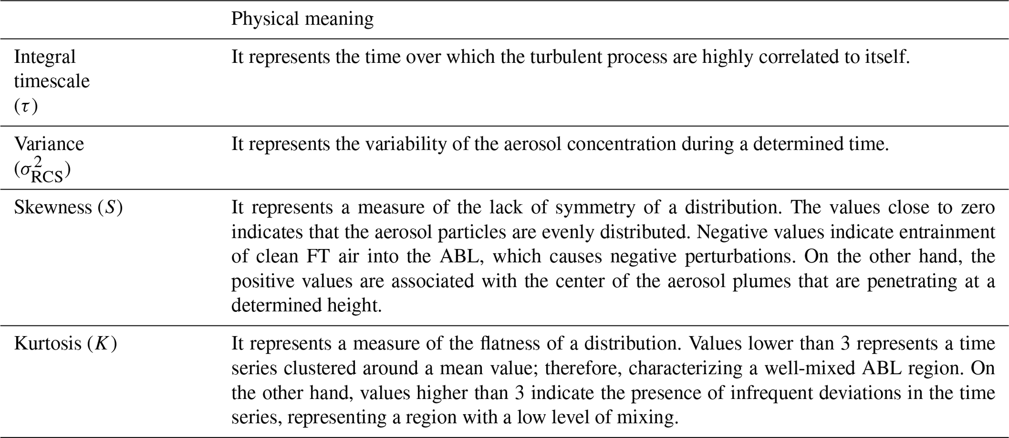
The high-order moments used in this study are obtained from RCS${}^{\prime }(z,t)$, generated by Eq. (1), where $\stackrel{\mathrm{‾}}{\mathrm{RCS}}\left(z\right)$ represents the 1 h average package of RCS(z,t) data. From this, the high-order moments, variance (σ²), skewness (S) and kurtosis (K) are obtained as demonstrated in the first column of Table 1, as well as their corrections and errors in the second and third columns of the same table, respectively. In Table 2 the physical meaning of each high-order moment in the context of the proposed analysis is presented.

Table 1Variables applied to statistical analysis of turbulence in the ABL region (Lenschow et al., 2000). The sum of subindex of autocovariance function M_ij represents the order of the analysis.

Download Print Version | Download XLSX

Table 2Physical meaning of the high-order moments

Download Print Version | Download XLSX

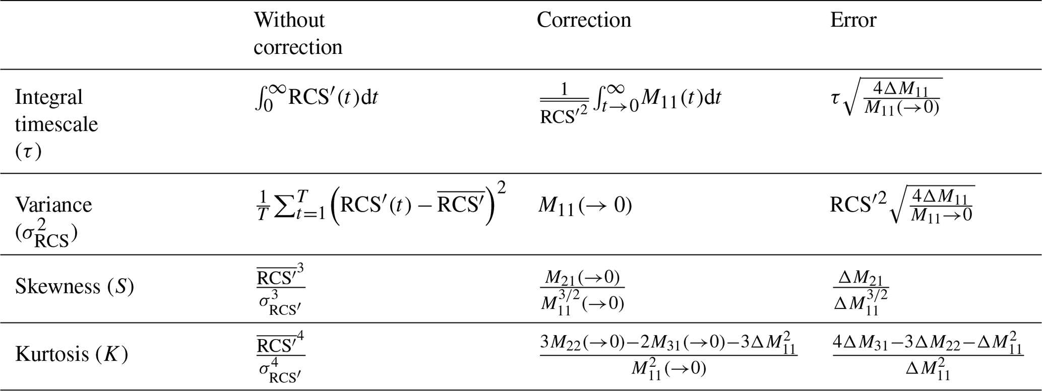
The integral timescale (τ) is an important prerequisite in turbulence studies. It guarantees that most of the horizontal variability of the turbulent eddies is detected with good resolution, enabling the solution of inertial subrange and dissipation range in the spectrum and autocorrelation function, respectively (Pal et al., 2010). τ must be larger than the temporal resolution of the analyzed time series (SPU lidar station time acquisition is 2 s). In the same way as the high-order moments, such variables are obtained from RCS${}^{\prime }(z,t)$, as shown in the first column of Table 1.

3.2 Error analysis

The high-order moments and τ generated from RCS${}^{\prime }(z,t)$ can also be obtained from the following autocovariance function M_ij, which has its order represented by the sum of the subscript i and j (Pal et al., 2010), according to the following equation:

where t_f means final time. However, it is important to consider the influence of instrument noise ε(z,t) in the RCS${}^{\prime }(z,t)$ profile. Therefore, M_ij can be rewritten as follows:

Although atmospheric fluctuations are correlated in time, ε(z,t) is random and uncorrelated with the atmospheric signal; therefore, ε(z,t) is only associated with lag zero. Consequently, it is possible to obtain the corrected autocovariance function, M₁₁(→ 0), removing the error ΔM₁₁(0) of the uncorrected autocovariance function M₁₁(0), as demonstrated in the equation below:

Based on this concept, Lenschow et al. (2000) proposed two methods to correct for the noise influence:

• First lag correction: the lag zero (ΔM₁₁(0)) is directly subtracted from the uncorrected autocovariance function M₁₁(0), generating M₁₁(→0).

• Two-thirds correction: a new lag zero value is obtained by the extrapolation of M₁₁(0) to the first nonzero lag back to lag zero, using the inertial subrange hypothesis (Monin and Yaglom, 1979):

  $$\begin{array}{}\text{(10)}& M_{\mathrm{11}}(\to \mathrm{0})=\stackrel{\mathrm{‾}}{RCS{}^{\prime }(z,t)}+C{t}^{\mathrm{2}/\mathrm{3}},\end{array}$$

  where C represents a parameter of turbulent eddy dissipation rate. In this study, we also used the first five points after lag zero to perform this correction. In Table 1 the second and third columns present the corrections and errors, respectively, of high-order moments and τ.

Figure 1Methodological description of data analysis performed for elastic lidar data.

Download

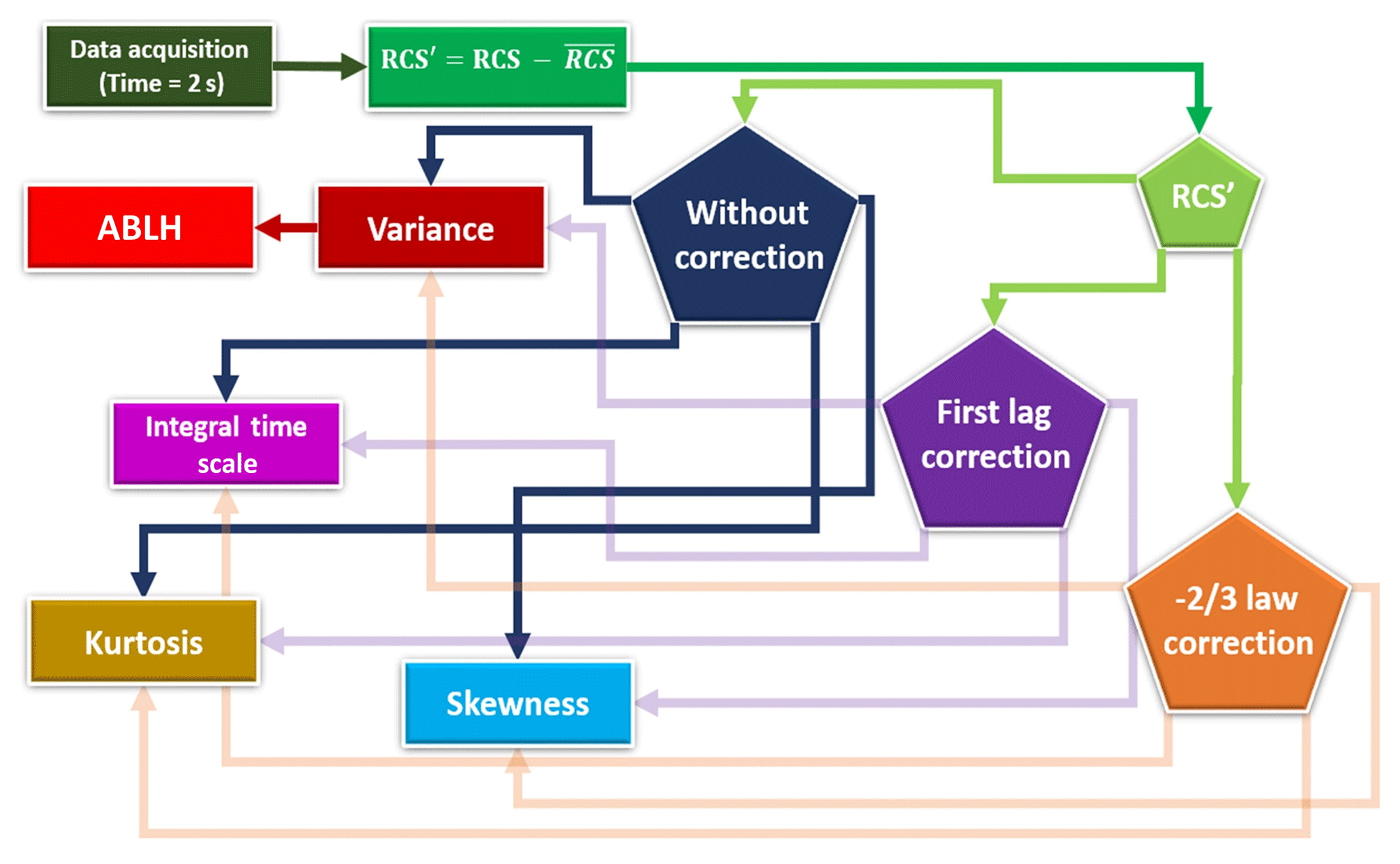
Figure 1 shows how the procedures described in Sect. 3.1 and 3.2 are used. Firstly, the lidar data are acquired with a time resolution of 2 s. Then, these data are averaged in packages of 1 h (the influence of the time window is demonstrated in de Arruda Moreira et al., 2019) generating $\stackrel{\mathrm{‾}}{\mathrm{RCS}\left(z\right)}$, from which it is possible to obtain RCS${}^{\prime }(z,t)$, as illustrated in Eq. (1). Then, the two corrections shown in Sect. 3.2 are separately applied. Finally, the high-order moments and the τ, corrected and without correction, are estimated. The ABLH is estimated from the variance method, which establishes, in convective conditions, the top of CBL (ABLH) as the maximum of the variance of the RCS [${\mathit{\sigma }}_{\mathrm{RCS}}^{\mathrm{2}}\left(z\right)$] (Baars et al., 2008). Examples of the application of such a methodology in varied meteorological scenarios (presence of clouds and aerosol sublayers) are presented in de Arruda Moreira et al. (2019).

4.1 Case study I: 26 July 2017

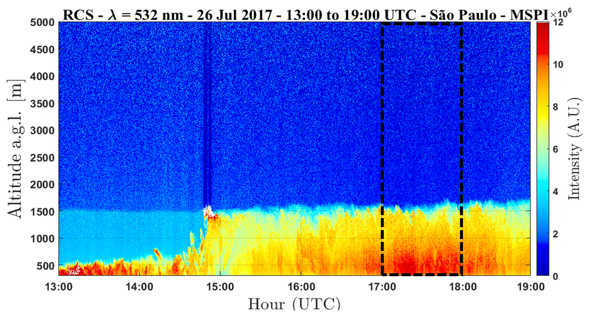
In this case study we gathered measurements from 13:00 to 19:00 UTC. Figure 2 shows the time–height plot of RCS₅₃₂ during this period. This case is composed of two distinct periods, in the first 2 h there is an RL with an underlying shallow CBL. Nevertheless, in the last part of the second hour the CBL quickly grows and it mixes with RL, forming a fully developed ABL, with its top situated between 1500 and 1600 m from 15:00 to 19:00 UTC. The dotted black box between 17:00 and 18:00 UTC represents the period selected to perform the statistical analysis.

In order to check the hypothesis proposed by Pal et al. (2010), which assumes that there is not particle hygroscopic growth and that the same type of aerosol is present in the entire atmospheric column in the ABL region, we analyzed the relative humidity and mixing ratio profile retrieved from radio-sounding measurements (http://weather.uwyo.edu/upperair/sounding.html, last access: 25 September 2018), launched at the Campo de Marte Airport (São Paulo, Brazil), which is about 10 km away from the SPU lidar system. Figure 3a and b show the relative humidity and mixing ratio profiles, respectively, measured on 26 Jul 2017 at 12:00 UTC. Both relative humidity and mixing ratio can be considered constant below 1500 m, with mean values of 67±8 % and 7.6±0.9 g kg⁻¹, respectively. Since there is no large variation in water vapor mixing ratio and relative humidity values in this region, we assume that this case is not affected by particle hygroscopic growth. In addition, the AERONET Sun photometer (Holben et al., 1998a) data from the São Paulo station were retrieved in order to check the aerosol type, as can be seen in Fig. 3c.

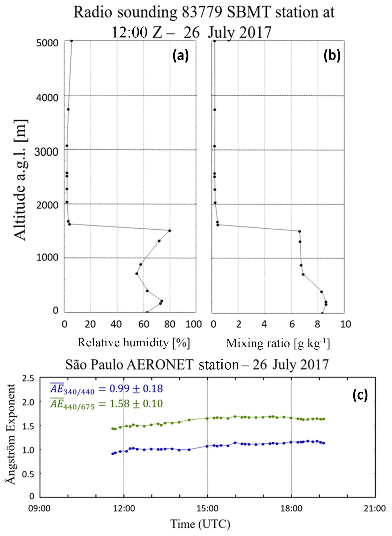
Figure 3(a) Vertical profile of relative humidity derived from radio sounding. (b) Mixing ratio derived from radio sounding. (c) Aerosol-optical-depth-related Ångström exponent time series from AERONET, for measurements retrieved at 26 July 2017.

Download

According to Eck et al. (1999), the Ångström exponent (AE) can be a useful tool for distinguishing different types of atmospheric aerosols. Figure 3c shows the aerosol AE time series for the case study of 26 July 2017. The AE was calculated at the spectral range 340–440 and 440–675 nm using AERONET (Holben et al., 1998b) products from level 1.5 version 3 data. For this measurement period, the percentage variation in AE was no more than 3 % in both cases. Therefore, there are no considerable changes during the whole measurement period, which is a strong indication that there is no aerosol type change throughout the day.

In Fig. 4 the signal-to-noise-ratio (SNR) profile of the raw lidar signal is presented, as calculated by Heese (2010) at three wavelengths (1064 nm, red line; 532 nm, green line; and 355 nm, violet line) during the analyzed period. All wavelengths have values of SNR higher than 1 (the threshold for good quality) below the ABLH (dotted blue line) with a predominance of values lower than 1 in the free troposphere (FT), which was expected due to the strong reduction of aerosol concentration in such region. Although the three wavelengths have similar SNR profiles, close to ABLH the differences among them become more evident, principally the fast decreasing of the 355 nm and the high values of 532 nm.

Figure 4Signal-to-noise-ratio (SNR) profile of the three wavelengths (1064 nm, red line; 532 nm, green line; and 355 nm, violet line) obtained at 26 July 2017 between 17:00 and 18:00 UTC.

Download

Figure 5 shows the autocovariance function (ACF), obtained between 17:00 and 18:00 UTC for the wavelengths 355 (ACF₃₅₅), 532 (ACF₅₃₂) and 1064 nm (ACF₁₀₆₄) at 1000 and 1700 m a.g.l. Thus, from the comparison of Figs. 2 and 5 it is possible to observe that the altitude chosen at 1000 m (red line) is situated below the top of CBL, while the altitude chosen at 1700 m (light green line) is in the FT. As expected, the ε, which is represented by the peak on the lag zero of the autocovariance function (5), increases with height for all the wavelengths due to reduction of aerosol load with height. ACF₃₅₅ has the lowest intensity (around 90 % smaller those of ACF₅₃₂ and ACF₁₀₆₄) and is clearly much more affected by the magnitude of ε that represents approximately 25 % of ACF₃₅₅, while for ACF₅₃₂ and ACF₁₀₆₄ the noise represents around 10 % of the respective autocovariance.

Figure 6 presents all statistical variables, their respective corrections and errors (shadows), generated from the methodology described in Sect. 3 for data acquired between 17:00 and 18:00 UTC.

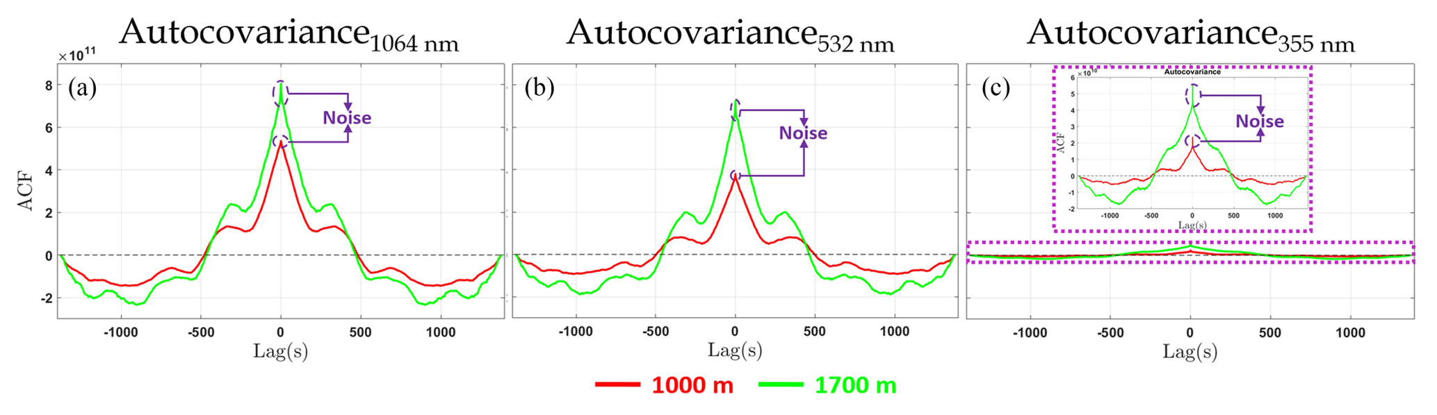
Figure 5Autocovariance function at 1064 nm (a), 532 nm (b) and 355 nm (c) on 26 July 2017 from 17:00 to 18:00 UTC. For 355 nm the insert magnifies the signal 10x.

Download

The variance profiles, ${\mathit{\sigma }}_{\mathrm{RCS}}^{\mathrm{2}}\left(z\right)$, with and without corrections for all wavelengths are represented in Fig. 6.01–.09. The low and almost constant values of uncorrected ${\mathit{\sigma }}_{{\mathrm{RCS}}_{\mathrm{1064}}}^{\mathrm{2}}\left(z\right)$ from the bottom up to around 1000 m in altitude demonstrates an almost constant distribution of aerosol particles in this region, as can be seen in Fig. 6.01. Above 1000 m in altitude, the value of uncorrected ${\mathit{\sigma }}_{{\mathrm{RCS}}_{\mathrm{1064}}}^{\mathrm{2}}\left(z\right)$ increases, reaching its maximum peak at around 1600 m. This peak represents the entrainment zone, the region where a mixing occurs between air parcels coming from the CBL and FT. According to Menut et al. (1999), there is an intense variation in aerosol concentration during this process, generating a maximum in the uncorrected ${\mathit{\sigma }}_{{\mathrm{RCS}}_{\mathrm{1064}}}^{\mathrm{2}}\left(z\right)$, which represents the ABLH. Above the ABLH, the aerosol concentration is considerably lower than in CBL and thus the uncorrected ${\mathit{\sigma }}_{{\mathrm{RCS}}_{\mathrm{1064}}}^{\mathrm{2}}\left(z\right)$ is reduced to practically zero. This methodology for estimating the ABLH is named the variance method or centroid method and it was described by Hooper and Eloranta (1986) and Menut et al. (1999), respectively. The main limitations of this method are its applicability only for CBL and the ambiguous results in complex cases, such as the presence of several aerosol layers (Emeis, 2011). In such situations more sophisticated methods like Wavelet (Pal et al., 2010), PathfinderTURB (Poltera et al., 2017) and POLARIS (Bravo-Aranda et al., 2017) are recommended.

The uncorrected ${\mathit{\sigma }}_{{\mathrm{RCS}}_{\mathrm{532}}}^{\mathrm{2}}\left(z\right)$, presented in Fig. 6.04, is rather similar to uncorrected ${\mathit{\sigma }}_{{\mathrm{RCS}}_{\mathrm{1064}}}^{\mathrm{2}}\left(z\right)$, including the position of maximum peak. Nevertheless, although uncorrected ${\mathit{\sigma }}_{{\mathrm{RCS}}_{\mathrm{355}}}^{\mathrm{2}}\left(z\right)$, presented in Fig. 6.07, also has the maximum peak situated at around 1600 m in altitude, the profile is noisier than the profiles obtained from the other wavelengths and, therefore, it is not possible to identify the regions with uniform aerosol distribution as evidenced in uncorrected ${\mathit{\sigma }}_{{\mathrm{RCS}}_{\mathrm{1064}}}^{\mathrm{2}}\left(z\right)$. Although the ${\mathit{\sigma }}_{{\mathrm{RCS}}_{\mathrm{355}}}^{\mathrm{2}}\left(z\right)$ is noisier than another ones, there is a low difference among the ABLH estimated from the three different wavelengths (lower than 10 %).

The two-thirds correction, shown in Fig. 6.02, 6.05 and 6.08, does not cause significant changes in the uncorrected profiles. On the other hand, the first lag correction significantly changes the profiles, thus ${\mathit{\sigma }}_{{\mathrm{RCS}}_{\mathrm{532}}}^{\mathrm{2}}\left(z\right)$ becomes very similar to ${\mathit{\sigma }}_{{\mathrm{RCS}}_{\mathrm{1064}}}^{\mathrm{2}}\left(z\right)$, while ${\mathit{\sigma }}_{{\mathrm{RCS}}_{\mathrm{355}}}^{\mathrm{2}}\left(z\right)$ continues with some differences, mainly in the region below the ABLH, as can be seen in Fig. 6.03, 6.06 and 6.09.

The integral timescale profiles ${\mathit{\tau }}_{\mathrm{RCS}{}^{\prime }}\left(z\right)$, with and without corrections, ${\mathit{\tau }}_{\mathrm{RCS}{}^{\prime }}^{\mathrm{corr}}\left(z\right)$ and ${\mathit{\tau }}_{\mathrm{RCS}{}^{\prime }}^{\mathrm{unc}}\left(z\right)$, respectively, calculated for the three wavelengths are presented in Fig. 6.10–.18. The ${\mathit{\tau }}_{\mathrm{RCS}{}^{\prime }}^{\mathrm{unc}}\left(z\right)$ presents values larger than SPU lidar station time acquisition, shown as a dotted black line in the region below ABLH at all wavelengths, as can be seen in Fig. 6.10, 6.13 and 6.16. The largest values of ${\mathit{\tau }}_{\mathrm{RCS}{}^{\prime }}^{\mathrm{unc}}\left(z\right)$ correspond to 1064 nm, while the lowest values are computed for 355, which is practically half of those obtained with the reference wavelength, 1064 nm. The low value for the ${\mathit{\tau }}_{\mathrm{RCS}{}^{\prime }}^{\mathrm{unc}}\left(z\right)$ at 355 nm can be associated with the influence of the noise in the signal retrieved at this wavelength. The application of the two-thirds correction does not cause significant changes in the profiles, while the first lag correction changes the profiles significantly mainly in the region below the ABLH, as can be seen in Fig. 6.11, 6.14 and 6.17 and in Fig. 6.12, 6.15 and 6.18, respectively.

The skewness profiles S_RCS(z) represent the degree of asymmetry in a distribution, where S_RCS(z)=0 represents symmetric distributions around its mean, while positive and negative values represent cases where the tail of distribution is on the left and right side of the distribution, respectively. The uncorrected skewness profiles $S_{\mathrm{RCS}}^{\mathrm{unc}}\left(z\right)$ and their respective corrections $S_{\mathrm{RCS}}^{\mathrm{corr}}\left(z\right)$ for the three wavelengths are presented in Fig. 6.19–.27. The $S_{\mathrm{RCS}}^{\mathrm{unc}}\left(z\right)$ generated from the wavelengths 1064 and 532 nm, presented in Fig. 6.19 and 6.22, respectively, presents similar behavior up to approximately 150 m above the ABLH_elastic, with positive values in the low part of the profile and one inflection point close to ABLH_elastic. Such a point characterizes the transition from the region with entrainment of clean FT air into the CBL (negative values) to a region a few meters above the ABLH_elastic with the presence of aerosol plumes (positive values) due to convective movement. This behavior of the skewness profile was also observed by Pal et al. (2010) and McNicholas and Turner (2014) at the region of the ABLH_elastic. Therefore, the same set of phenomena is evidenced by the dataset at both wavelengths, although there are differences in the absolute values.

The two corrections cause negligible variations in the profiles at 1064 nm, as shown in Fig. 6.20 and 6.21. On the other hand, the corrections applied to the $S_{\mathrm{RCS}}^{\mathrm{unc}}\left(z\right)$ at 532 nm produce skewness profiles similar to those at the reference wavelength, as can be seen in Fig. 6.23 and 6.24. It is possible to observe a difference between the skewness profiles at 532 nm (positive) and 1064 nm (negative) in the region above the ABLH_elastic. Such difference is a consequence of the low values of signal-to-noise ratio (SNR) of the RCS' and consequently τ_RCS(z) observed in this region, preventing the observation of turbulence due to the technical limitations of the instruments used. The skewness profiles at 355 nm, $S_{\mathrm{RCS}}^{\mathrm{corr}}\left(z\right)$ and $S_{\mathrm{RCS}}^{\mathrm{unc}}\left(z\right)$ present a rather different behavior and do not follow the same variations observed in the reference wavelength profile, as can be seen in Fig. 6.25, 6.26 (two-thirds correction) and 6.27 (first lag correction). Consequently, it is not possible to observe the aerosol dynamics using the information gathered at the wavelength 355 nm.

The kurtosis profile $K_{\mathrm{RCS}{}^{\prime }}$ is the most complex high-order moment presented in this study and, consequently, in such profiles the differences among the three wavelengths are more evident. In the context of our analysis, the values of $K_{\mathrm{RCS}{}^{\prime }}$ are indicators of the mixing degree at each altitude, as well as of the intermittence of turbulence caused by large eddies. Because of some technical limitations of our lidar system, it is possible to resolve eddies only up to a predetermined size. Therefore, in regions where turbulence is performed in overly small scales, our system cannot solve these eddies. The kurtosis equation presented in the Table A1 represents the kurtosis of a normal distribution, which is equal to 3 (Bulmer, 1965). Consequently, such a value is applied as a threshold in the analyses performed in this paper. Values lower than 3 represent a well-mixed region, indicating a flatter distribution in comparison to a normal distribution, thus the turbulence caused by large eddies can be characterized as frequent. In contrast, values higher than 3 indicate a peaked distribution in comparison to a Gaussian distribution. In other words, there is an unusual variation in the RCS${}^{\prime }(z,t)$, which represents a low degree of mixing and the presence of an infrequent large eddy turbulence (Pal et al., 2010).

The $K_{\mathrm{RCS}{}^{\prime }}^{\mathrm{unc}}$ at 532 and 1064 nm have some differences in the region below 1300 m in altitude, where the profile at 1064 nm only shows values higher than 3, representing a region with a low degree of mixing, while the $K_{\mathrm{RCS}{}^{\prime }}^{\mathrm{unc}}$ obtained from 532 nm is composed of values higher and lower than 3. From 1300 to 3500 m in altitude, the profiles of these two wavelengths are very similar, with values lower than 3 in the region below the ABLH, characterizing a well-mixed region, a peak of values higher than 3 in the first meters above the ABLH, and values between 3 and 4 in the remainder of the profile. The corrections do not cause significant changes in the 1064 nm kurtosis profile, as can be seen in Fig. 6.29 and 6.30. However, the variation in the kurtosis profile at 532 nm is remarkable, as presented in Fig. 6.32 and 6.33. Thus, it becomes very similar to the 1064 nm profile, mainly with the use of first lag correction. The $K_{\mathrm{RCS}{}^{\prime }}^{\mathrm{unc}}$ obtained from 355 nm does not have the same variations observed in the profiles obtained at the reference wavelength. Therefore, it is not possible to identify the occurrence of the phenomena previously described. The same problem occurs in the $K_{\mathrm{RCS}{}^{\prime }}^{\mathrm{corr}}$, although the application of corrections causes relevant variations in relation to values observed in $K_{\mathrm{RCS}{}^{\prime }}^{\mathrm{unc}}$.

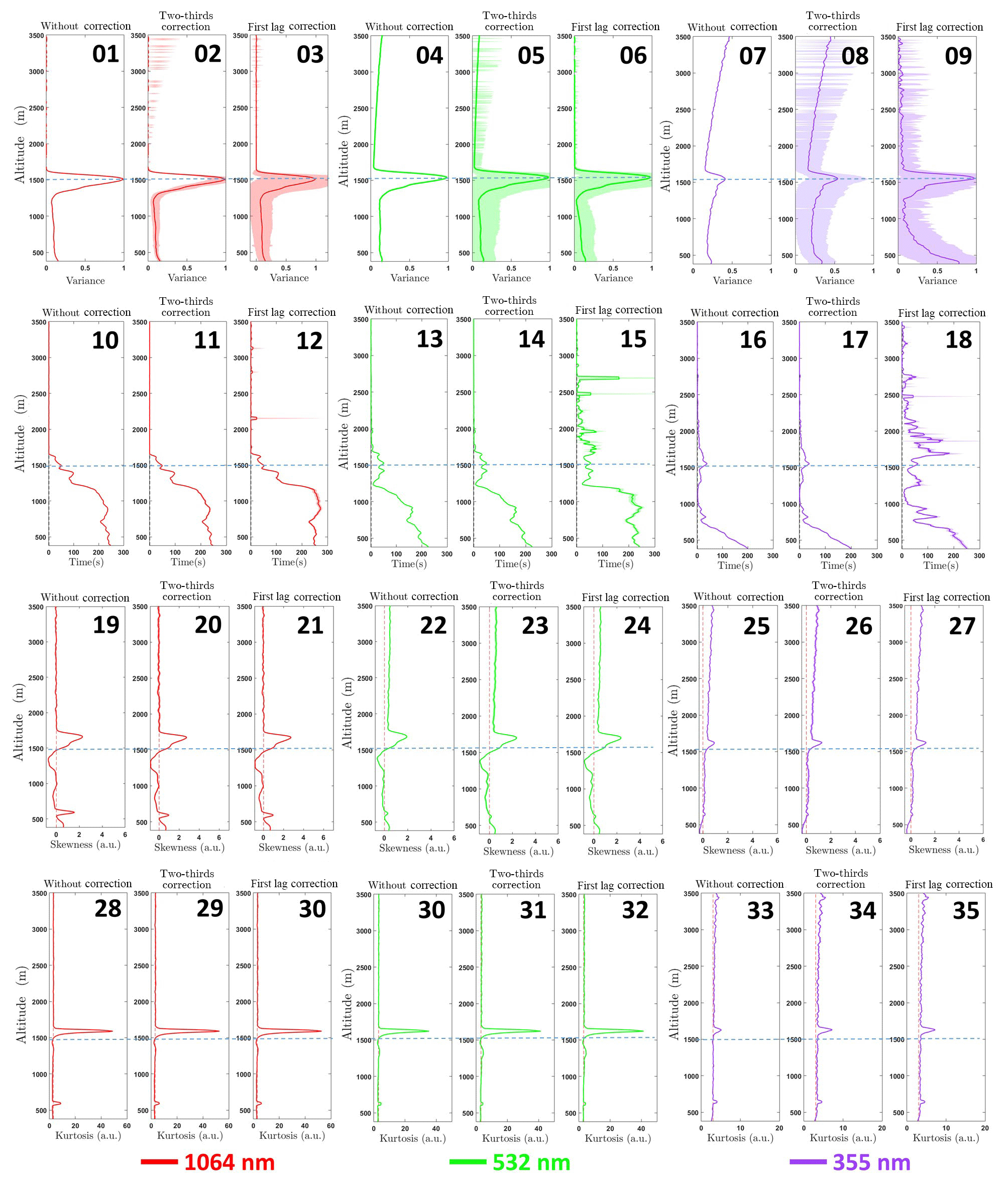
Figure 6High-order moments and τ without correction and corrected by the two-thirds law and first lag correction at 1064 (red line), 532 (green line) and 355 nm (violet line) on 26 July 2017 from 17:00 to 18:00 UTC. The horizontal dotted blue line represents the ABLH_elastic.

Download

Figure 7 shows the profiles of β_mol, β_mol+aer and β_ratio of the wavelengths 1064 nm (Fig. 7.1 and 7.2), 532 nm (Fig. 7.3 and 7.4) and 355 nm (Fig. 7.5 and 7.6). Such profiles were obtained from the data retrieved during the period of analysis presented previously. From Fig. 7.1 it is possible to observe the predominance of β_aer in the wavelength 1064 nm and because of this the β_ratio presented in Fig. 7.2 achieved large values. In Fig. 7.3 it is possible to observe the predominance of β_aer in the wavelength 532 nm and a small impact of β_mol. The backscatter profile at 355 nm presented in Fig. 7.5 shows that both β_aer and β_mol, have the same order of magnitude but with a predominance of β_aer. Such profiles justify the differences and similarities observed in the results obtained from each wavelength. Although the backscatter profiles at 532 nm are composed of the molecular and aerosol signatures, the predominance of the latter enables the observation of the phenomena presented by high-order moment profiles obtained from the reference wavelength. The small presence of β_mol can also be an indicator of the low values of noise, although they are higher than the values of reference wavelength.

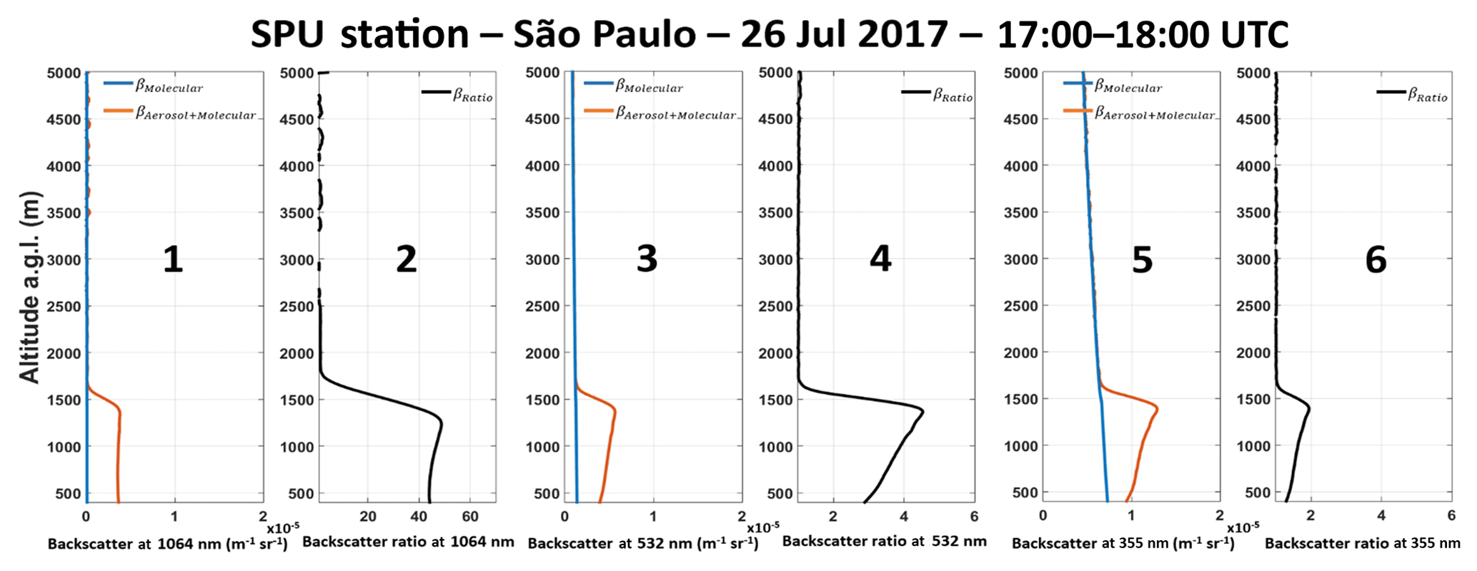
Figure 7Total (aerosol and molecular) backscatter profile and backscatter ratio retrieved using the Klett–Fernald–Sasano inversion technique for 1064, 532 and 355 nm, respectively, for data retrieved on 26 July 2017 at 17:00–18:00 UTC by the SPU lidar system.

Download

4.2 Case study II: 19 July 2018

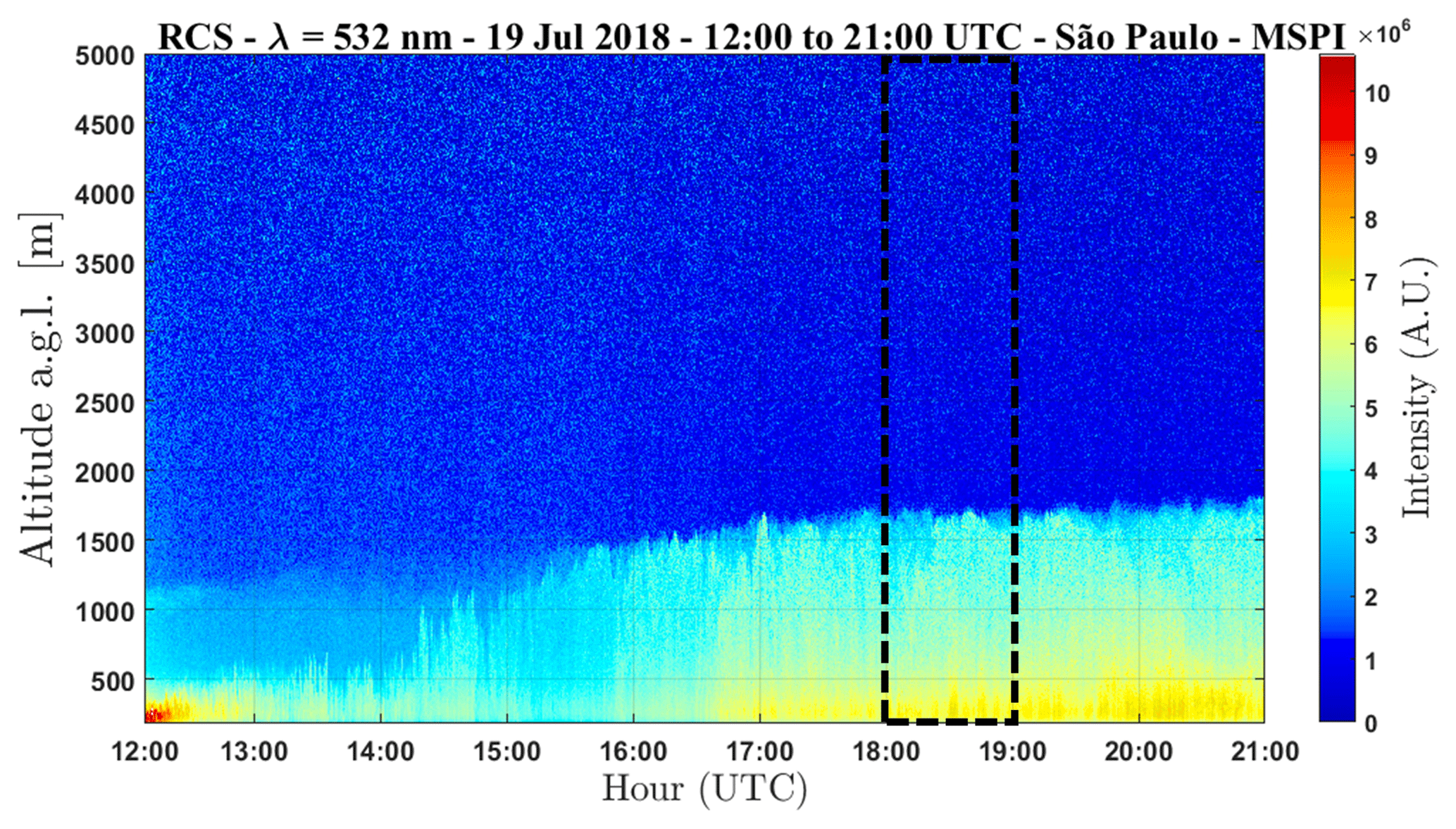
In this case study measurements were gathered with the SPU lidar station from 12:00 to 21:00 UTC. Figure 8 shows the time–height plot of RCS₅₃₂ during this period (the time–height plot of the RCS₃₅₅ and RCS₁₀₆₄ are available in the Supplement as Figs. S1 and S2, respectively). At the beginning of measurement it is possible to observe the presence of an ascending CBL covered by a RL, which has the top situated at around 1300 m in altitude. At approximately 15:30 UTC the CBL breaks up the RL and becomes fully developed, thus its growth speed is reduced and the value of top height remains practically constant (1600 m) from 17:00 UTC until 21:00 UTC. The dotted black box in Fig. 8 represents the chosen period for performing the statistical analysis (18:00–19:00 UTC).

Figure 8Time–height plot of RCS₅₃₂.

Download

In the same way as case study I, the hypothesis proposed by Pal et al. (2010) is validated from the profiles presented in Fig. 9 (more information are available in the Suplement as Fig. S3). The profiles of relative humidity and mixing ratio, presented in Fig. 9a and b, respectively, do not have large variations in the CBL below 1200 m in altitude. In addition, the aerosol-optical-depth-related Ångström exponent time series did not show considerable changes during the whole measurement period, as can be seen in Fig. 9c. For this measurement period the percentage variation in AE was no more than 4 % and 3 % in the spectral range 340–440 and 440–675 nm, respectively. Therefore, there are no considerable changes during the whole measurement period, which is a strong indication that there are no aerosol type change throughout the day and the atmospheric conditions are not propitious for particle hygroscopic growth events.

Figure 10 presents the SNR profile of the raw lidar signal of the three wavelengths (1064 nm; red line; 532 nm, green line; and 355 nm, violet line) during the analyzed period. In the ABL region, all wavelengths have similar profiles with values higher than 1. However, as ABLH approaches, the values of SNR reduce sharply, mainly at 355 nm. Consequently, in the FT region all profiles have values lower than 1, as expected.

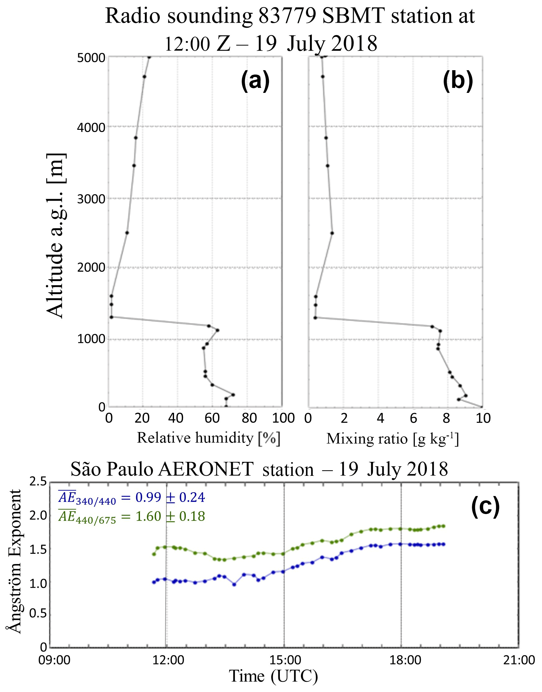
Figure 9(a) Vertical profile of relative humidity derived from radio sounding. (b) Mixing ratio derived from radio sounding. (c) Aerosol-optical-depth-related Ångström exponent time series from AERONET, for measurements retrieved at 19 July 2018.

Download

Figure 11 shows a comparison among the ACF obtained from the three wavelengths 1064 nm (Fig.11a), 532 nm (Fig.11b) and 355 nm (Fig.11c), between 18:00 and 19:00 UTC at two heights: 1000 m (red line) and 1700 (green line). In the same way as case study I, the region above ABLH (green line) is more influenced by noise than the region situated below this height (red line). The intensity of ACF₅₃₂ and ACF₁₀₆₄ are very similar, although the presence of noise in the former, which is 40 % and 46 %, below and above ABLH, respectively, is higher than in the latter, 27 % and 30 %, below and above ABLH, respectively. The ACF₃₅₅ presents a lower intensity value in comparison to the other two wavelengths and a strong presence of noise below and above the ABLH, 50 % and 67 %, respectively.

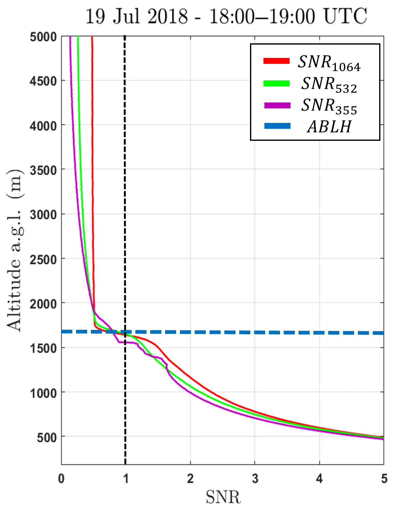
Figure 10Signal-to-noise-ratio (SNR) profile of the three wavelengths (1064 nm; red line, 532 nm green line; and 355 nm, violet line) obtained on 19 July 2018 between 18:00 and 19:00 UTC.

Download

The three high-order moments and τ_RCS, both corrected by the first lag correction and obtained between 18:00 and 19:00 UTC, are presented in Fig. 12. The ${\mathit{\tau }}_{\mathrm{RCS}}^{\mathrm{corr}}$ for all wavelengths has values higher than 2 s from the bottom of profile up to the first meters above the ABLH_elastic with a maximum of ${\mathit{\sigma }}_{\mathrm{RCS}{}^{\prime }}^{\mathrm{2}}\left(z\right)$. Although the values obtained from 1064 nm and 532 nm are almost twice as large as the values generated from 355 nm (in the same way as case study I), there are some differences among the maxima of the [${\mathit{\sigma }}_{\mathrm{RCS}}^{\mathrm{2}}\left(z\right)$] and they do not significantly influence the ABLH estimation, thus the difference among the ABLH obtained from each wavelength is lower than 10 %. The positive values of $S_{\mathrm{RCS}}^{\mathrm{corr}}\left(z\right)$ of 1064 nm indicate the presence of aerosol updrafts from the bottom of the profile up to around 750 m in altitude. From this height up to the ABLH, the $S_{\mathrm{RCS}}^{\mathrm{corr}}\left(z\right)$ is characterized by negative values, which represents a region with entrainment of clean FT air into the CBL. In the same way as case study I, there is an inflection point at ABLH, which reproduces the transition from negative to positive values, the latter values indicating the presence of aerosol updraft layers in the first 200 m above the ABLH. Such behavior in the region of ABLH was also observed by Pal et al. (2010) and McNicholas and Turner (2014) and can be considered characteristic of convective regime. The $S_{\mathrm{RCS}}^{\mathrm{corr}}\left(z\right)$ obtained from the wavelengths 1064 and 532 nm presents an identical pattern of behavior, demonstrating the occurrence of the same phenomena. The $S_{\mathrm{RCS}}^{\mathrm{corr}}\left(z\right)$ obtained from the wavelength 355 nm, in the same way as the previous case study, does not exhibit the behavior observed in the reference wavelength, presenting only positive values in the whole profile. Therefore, it is not possible to identify variations in the aerosol dynamic using 355 nm.

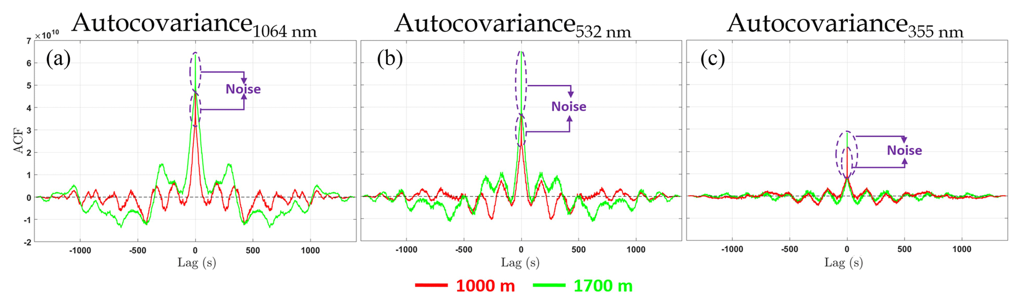
Figure 11Autocovariance function at 1064 (a), 532 (b) and 355 nm (c) on 19 July 2018 from 18:00 to 19:00 UTC.

Download

The $K_{\mathrm{RCS}}^{\mathrm{corr}}\left(z\right)$ obtained from the wavelength 1064 nm presents values higher than 3 from the bottom up to around 1300 m in altitude, characterizing a region with a low degree of mixing. From 1300 m up to the ABLH the $K_{\mathrm{RCS}}^{\mathrm{corr}}\left(z\right)$ has values lower than 3, which characterize this region as showing a large degree of mixing and (in a more evident way) the presence of turbulence. Such behavior occurs mainly due to entrainment of cleaner air. A few meters above the ABLH, the $K_{\mathrm{RCS}}^{\mathrm{corr}}\left(z\right)$ has a great peak, which occurs due to rare aerosol plumes penetrating at this region. Such behavior was also observed in case study I, as well as by Pal et al. (2010) and McNicholas and Turner (2014). Above the ABLH the profile only has values higher than 3; however, as ${\mathit{\tau }}_{\mathrm{RCS}}^{\mathrm{corr}}\left(z\right)$ decreases to values close to zero and low values of SNR of the RCS are characteristic of this region, it is not possible to extract conclusive information from $K_{\mathrm{RCS}}^{\mathrm{corr}}\left(z\right)$. In the same way as the comparison performed with other variables, the $K_{\mathrm{RCS}}^{\mathrm{corr}}\left(z\right)$ obtained from the wavelength 532 nm presents similar behavior to the profile obtained from 1064 nm, thus the same phenomena can be observed. On the other hand, the $K_{\mathrm{RCS}}^{\mathrm{corr}}\left(z\right)$ obtained from the wavelength 355 nm does not allow for observing the behavior detected in the profile obtained from the reference wavelength because along the whole profile the $K_{\mathrm{RCS}}^{\mathrm{corr}}\left(z\right)$ at 355 nm presents values higher than 3.

Figure 12High-order moments corrected by first lag correction at 1064 (red line), 532 (green line) and 355 nm (violet line) on 19 July 2018 from 18:00 to 19:00 UTC.

Download

Figure 13 shows the composition signal of β_aer and β_mol, retrieved during the analyzed period of this case study (18:00–19:00 UTC) using the Klett–Fernald–Sasano inversion (Klett, 1983, 1985; Fernald, 1984; Sasano and Nakane, 1984), at each one of the three wavelengths, as well as the β_ratio calculated using the backscatter profile of aerosol and molecular component (Bucholtz, 1995). From Fig. 13.1 it is possible to observe that the backscattered signal at 1064 nm has a predominance of β_aer, with almost null values of β_mol. The composition of the backscattered signal at 532 nm is shown in Fig. 13.3. Although the component β_mol has values higher than the ones observed in wavelength 1064 nm, the component β_aer is predominant in the backscattered signal composition. The backscattered signal at 355 nm, presented in Fig. 13.5, unlike the other wavelengths, is predominantly composed of β_mol and has a low percentage of β_aer.

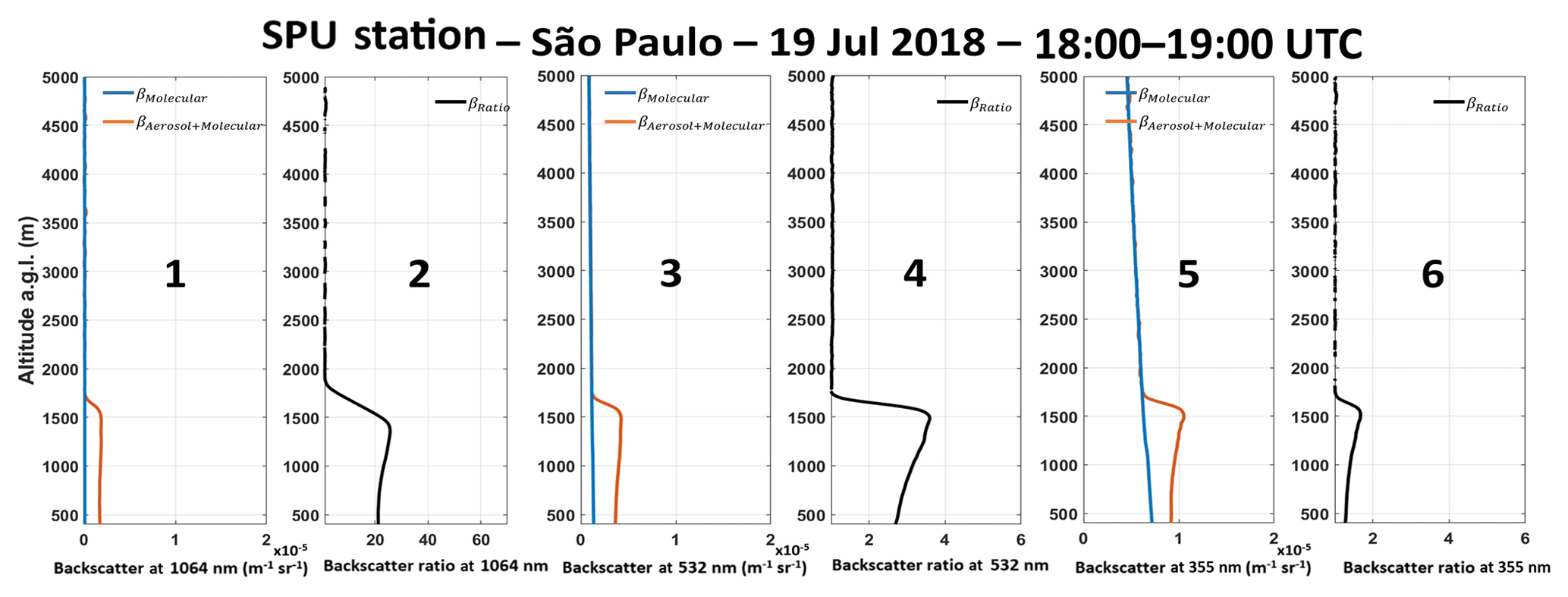
Figure 13Total (aerosol and molecular) backscatter profile and backscatter ratio retrieved using Klett–Fernald–Sasano inversion technique for 1064, 532 and 355 nm, respectively, for data retrieved on 19 July 2018 from 18:00 to 19:00 UTC.

Download

From the results obtained in both case studies, it is possible to observe the influence of the wavelength in the proposed methodology. The wavelength 1064 nm, considered our signal reference, has a negligible influence on component molecules; therefore, the backscatter signal retrieved at 1064 nm can be considered approximately equal to the backscatter signal retrieved only by the aerosol contribution, β₁₀₆₄ ≈ β_aer. Before taking into account the approximation demonstrated in Eq. (5) (RCS₁₀₆₄ ≈ β₁₀₆₄), we can conclude that the range-corrected signal retrieved from a lidar at 1064 nm can be considered, with good precision, approximately equal to the backscatter signal retrieved at the same wavelength for aerosol components, RCS₁₀₆₄ ≈ β_aer. Such a relation enables the observation of behavior of aerosol plumes from high-order moments. In the case of wavelength 532 nm, β₅₃₂ is composed of β_aer and β_mol (${\mathit{\beta }}_{\mathrm{532}}={\mathit{\beta }}_{{\mathrm{aer}}_{\mathrm{532}}}+{\mathit{\beta }}_{{\mathrm{mol}}_{\mathrm{532}}}$); however, as shown in Figs. 8 and 13, there is a predominance of β_aer. Although the high-order moment profiles obtained from the wavelength 532 nm are noisier than that one generated from the reference wavelength data, the phenomena observed from the 1064 nm data can also be observed in 532 nm data, mainly after the application of first lag correction. Consequently, the wavelength at 532 nm can be used in the proposed methodology providing satisfactory results. On the other hand, the backscatter at 355 nm is predominantly composed of β_mol and has a small percentage of β_aer, as presented in Figs. 8 and 13.

This fact justifies the low quality observed in the results retrieved using the wavelength of 355 nm. As established in Eq. (3), the turbulent variable is directly associated with $\mathit{\beta }{{}^{\prime }}_{\mathrm{aer}}$, but, due to the low contribution of this component in the backscatter signal at 355 nm, the supposition established in Eq. (6) cannot be applied. Consequently, the high-order moments obtained from the proposed methodology are noisier and the value of ${\mathit{\tau }}_{\mathrm{RCS}{}^{\prime }}\left(z\right)$ is almost half of the value obtained from the reference wavelength, both due to influence of β_mol that presents the stronger contribution to the total backscatter coefficient at this wavelength. Therefore, the behavior observed in the high-order moment profiles generated from the 1064 nm wavelength data can be detected as partially (or even totally) suppressed as the complexity of high-order moments increases. In both case studies it was possible to observe from the third-order moment (skewness) that the results obtained from the wavelength 355 nm provide misinformation.