the Creative Commons Attribution 4.0 License.
the Creative Commons Attribution 4.0 License.
 | 04 Sep 2019
Diurnal and nocturnal cloud segmentation of all-sky imager (ASI) images using enhancement fully convolutional networks
Chaojun Shi
Yatong Zhou
Bo Qiu
Jingfei He
Mu Ding
Shiya Wei
Cloud segmentation plays a very important role in astronomical observatory site selection. At present, few researchers segment cloud in nocturnal all-sky imager (ASI) images. This paper proposes a new automatic cloud segmentation algorithm that utilizes the advantages of deep-learning fully convolutional networks (FCNs) to segment cloud pixels from diurnal and nocturnal ASI images; it is called the enhancement fully convolutional network (EFCN). Firstly, all the ASI images in the data set from the Key Laboratory of Optical Astronomy at the National Astronomical Observatories of Chinese Academy of Sciences (CAS) are converted from the red–green–blue (RGB) color space to hue saturation intensity (HSI) color space. Secondly, the I channel of the HSI color space is enhanced by histogram equalization. Thirdly, all the ASI images are converted from the HSI color space to RGB color space. Then after 100 000 iterative trainings based on the ASI images in the training set, the optimum associated parameters of the EFCN-8s model are obtained. Finally, we use the trained EFCN-8s to segment the cloud pixels of the ASI image in the test set. In the experiments our proposed EFCN-8s was compared with four other algorithms (OTSU, FCN-8s, EFCN-32s, and EFCN-16s) using four evaluation metrics. Experiments show that the EFCN-8s is much more accurate in cloud segmentation for diurnal and nocturnal ASI images than the other four algorithms.


Cloud plays an important role in the Earth's thermal balance and water cycle, which is one of the important indicators for astronomical observatory site selection (Stephens, 2005). Cloud coverage and movements affect the time of astronomical observations. At present, cloud observations rely mainly on satellite remote sensing and ground-based observations. A detailed review has been given about the advantages and disadvantages of satellite remote sensing and ground-based observations (Tapakis and Charalambides, 2013). Satellite cloud images can provide large-scale distribution structure information on cloud in a wide range. Different types and distribution patterns of cloud can provide rich weather information, but the description accuracy of thin clouds and low cloud is not high enough to accurately reflect local weather conditions and changes in the atmosphere. The ground-based cloud observation range is small, and it can provide local information such as cloud block size and arrangement. It has the advantages of flexible observation points, easy operation, being convenient and fast, and producing mostly visible-light images, with rich image information. However, if relying on the experience of observers to perform manual observation, the observation result is easily restricted by human factors, resulting in a lack of objectivity and accuracy, and the automatic detection and recognition of cloud images cannot be realized. Therefore, the development of automated cloud detection and identification equipment has become an inevitable trend.
With the development of hardware technologies such as charge-coupled devices and digital image processing, many ground-based full-sky cloud-measuring instruments have been successfully developed. Currently, the most representative instruments include the Whole Sky Imager (WSI; Johnson et al., 1989), Total Sky Imager (TSI; Long and Deluisi, 1998; Long et al., 2006), Infrared Cloud Imager (ICI; Shaw et al., 2005; Thurairajah and Shaw, 2005; Nugent et al., 2009, 2013), All Sky Imager (ASI; Cazorla et al., 2008), Whole Sky Infrared Cloud Measuring System (WSIRCMS; Sun et al., 2008), Total Sky Cloud Imager (TCI; Yang et al., 2012), All-Sky Infrared Visible Analyzer (ASIVA; Klebe et al., 2014), Whole Sky Camera (WSC; Kuji et al., 2018), and All Sky Camera (ASC; Aebi et al., 2018). The above instruments provide hardware support for analyzing ground-based cloud images, making the automated observation of ground-based cloud images possible.
Benefiting from these cloud-measuring instruments, many ground-based cloud segmentation algorithms have appeared. Atmospheric molecular scattering is inversely proportional to the fourth power of the wavelength, and cloud particle scattering is not closely related to wavelength, so the sky is blue and the cloud appears white in daytime. Therefore, threshold algorithms have become the mainstream for ground-based cloud detection. Long et al. (2006) proposed a cloud detection algorithm based on color thresholds to extract the regions of the cloud using 0.6 as a single fixed threshold in red-to-blue (R∕B) ratio bands. Different from the ratio R∕B, Heinle et al. (2010) revamped the criterion and adopted using the difference value of R–B to segment clouds. Then, upper and lower thresholds for each attribute to segment the cloud were proposed, which are determined by the average and standard deviations of the saturation values (Souza-Echer et al., 2006). Yang et al. (2015) analyzed the imaging of color cameras and proposed a new algorithm, which is green-channel background subtraction adaptive threshold, to automatically detect cloud within ground-based total-sky visible images. Yang et al. (2016) proposed an improved total-sky cloud segmentation algorithm, clear-sky background differencing (CSBD), using a real clear-sky background to improve the cloud segmentation accuracy. To remove the difference of atmospheric scattering and obtain a homogeneous sky background, Yang et al. (2017) proposed a cloud segmentation algorithm using a new red–green–blue (RGB) channel operation by combining the advantages of the threshold and differencing algorithms.
Li et al. (2011) combined the fixed and adaptive threshold algorithm and proposed an effective cloud segmentation algorithm called the hybrid threshold algorithm (HTA). Ghonima et al. (2012) compared the pixel red–blue ratio (RBR) to the RBR of a clear-sky library (CSL) for more accurate cloud segmentation. Different from the various algorithms mentioned above, Calbo and Sabburg (2008) presented several features that are computed from the threshold image, extracted from statistical measurements of image texture, based on the Fourier transform of the image, and can be useful for cloud segmentation of all-sky images. Peng et al. (2015) designed a classifier-based pipeline of identifying and tracking clouds in three-dimensional space to utilize all three total-sky imagers for multisource image correction to enhance the overall accuracy of cloud detection. Shi et al. (2017) used a superpixel-based graph model (GM) to integrate multiple source information and proposed a new ground-based cloud detection algorithm to solve the problem that with a single information source, it is difficult to split the cloud from the clear sky. By analyzing components and different color spaces using partial least squares regression, Dev et al. proposed a supervised segmentation framework to segment ground-based cloud pixels without any manually defined parameters (Dev et al., 2017a). Neto et al. (2010) described a new segmentation algorithm using Bayesian inference and multidimensional Euclidean geometric distance to segment the cloud and sky patterns in image pixels on the RGB color space. Calbo et al. (2017) proposed sensitivity as the thin boundary between clouds and aerosols. Roman et al. (2017) presented a new cloud segmentation strategy using high dynamic range images from a sky camera and ceilometer measurements, which is also able to segment the obstruction of the sun. With the development of neural networks, algorithms in the field of deep learning (LeCun et al., 1989; Ning et al., 2005; Hinton and Salakhutdinov, 2006; Krizhevsky et al., 2017; Shelhamer et al., 2017) began to be applied to cloud segmentation. Moreover, Cheng and Lin (2017) segmented cloud using supervised learning with multi-resolution features. The features include multi-resolution information and local structure extracted from local image patches with different sizes.
The algorithms proposed above are all for segmenting cloud from total-sky images in the daytime. For nocturnal ASI images of cloud and sky background, pixel values are very low and difficult to distinguish. The effect of sunlight on nocturnal ASI images is very weak, but weak light such as moonlight and starlight have a great influence on it. Therefore, nocturnal ASI images are more noisy than diurnal ASI images. Gacal et al. (2016) proposed an algorithm to segment nocturnal cloud images using a single fixed threshold method. The algorithm uses temporal averaging to estimate cloud cover based on the segmentation results of images near the zenith. However, due to factors such as moonlight, lighting, and weather conditions, it is difficult to accurately segment cloud pixels by a single fixed threshold method. Dev et al. (2017b) proposed a superpixel-based algorithm to segment nocturnal sky–cloud images, and the first nocturnal sky–cloud image segmentation database was introduced to the public in their paper. Dev et al. (2019) first integrated diurnal and nocturnal image segmentation into one framework. They proposed a lightweight deep-learning architecture called CloudSegNet and achieved good results. However, so far, few researchers have segmented nocturnal cloud images. Accordingly, we propose a new automatic cloud segmentation algorithm that utilizes the advantages of deep-learning algorithm fully convolutional networks (FCNs); it is called an enhancement fully convolutional network (EFCN). Section 2 describes the ASI device and the data set of ASI images. Section 3 shows the proposed EFCN in detail. In Sect. 4, we conducted three sets of experiments to segment cloud pixels with the proposed algorithm and four other algorithms. Then we analyzed the experimental results in detail based on four evaluation metrics. Finally, Sect. 5 gives a summary and some suggestions for future work.
The cloud images used in this paper are taken by an ASI and provided by the Key Laboratory of Optical Astronomy at the National Astronomical Observatories of CAS. Figure 1a demonstrates the ASI device. Like other all-sky cloud-measuring instruments, the key equipment of the ASI includes a fish-eye lens, an industrial camera, and a clear glass cover. The device can cover a field of view larger than 180∘. The camera is protected by the clear glass cover to prevent damage by wind, rain, snow, and fog, and it can capture one 24-bit RGB color space ASI image per 3 s. The resolution of the original RGB color space ASI images is 2592×1728 pixels as shown in Fig. 1b. We randomly select 1124 original RGB color space ASI images to construct our data set, including 369 original diurnal ASI images and 755 original nocturnal ASI images. We define the original ASI images taken from 07:00 (UTC/GMT+08:00) the morning until 19:00 at night as diurnal ASI images and those taken from 19:00 at night until 07:00 the next morning as nocturnal ASI images. In the data set, we randomly select 1054 original RGB color space ASI images as the training set, including 343 original diurnal ASI images and 711 original nocturnal ASI images. Another 70 original ASI images in the data set are selected as the test set, with 26 original diurnal ASI images and 44 original nocturnal ASI images.
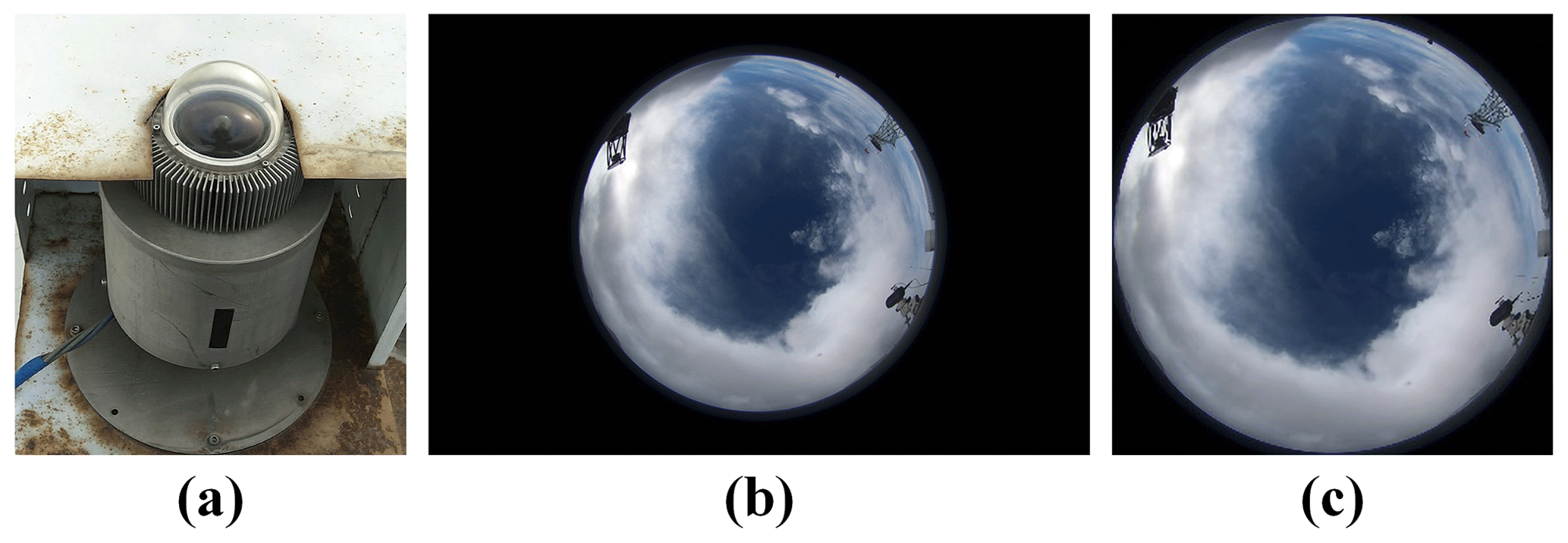
Figure 1ASI device and ASI image. (a) ASI device including a fish-eye lens, an industrial camera, and a clear glass cover. (b) Original RGB color ASI image (2592×1728 pixels) and (c) resized RGB color ASI image of (b) (1408×1408 pixels).
The effective area of the original RGB color space ASI images is a circular region with a diameter including 1408 pixels. Therefore, each image of the data set is resized into 1408×1408 pixels as shown in Fig. 1c. We manually label the pixels belonging to cloud of each resized ASI image in the training set and test set using the software LabelMe, creating the ground truth of the data set. We first open the image to be labeled in the software LabelMe. Second, we label the cloud pixels with multiple closed curves to ensure that the cloud pixels are inside the curve and the sky background is outside the curve. We then set the labeled cloud pixel to blue and the unlabeled sky background to black. A json file is generated after labeling. Finally, we convert the json file into a labeled image. Figure 2 shows eight diurnal and nocturnal resized RGB color space ASI images in the data set and the corresponding ground truth of the eight diurnal and nocturnal resized ASI images. Figure 2a shows the diurnal resized ASI images in the data set, and their corresponding ground truth is shown in Fig. 2b. Figure 2c denotes the nocturnal resized ASI images in the data set. Figure 2d presents the corresponding ground truth of the nocturnal resized ASI images from Fig. 2c. In Fig. 2b and c, white pixels indicate the cloud and black pixels indicate the sky background. The device used for training is a server equipped with a NVIDIA GeForce GTX 1080ti×2 with 11×2 GB memory. The deep-learning framework used in the experiments is TensorFlow, and the software programming environment is Python 3.5.
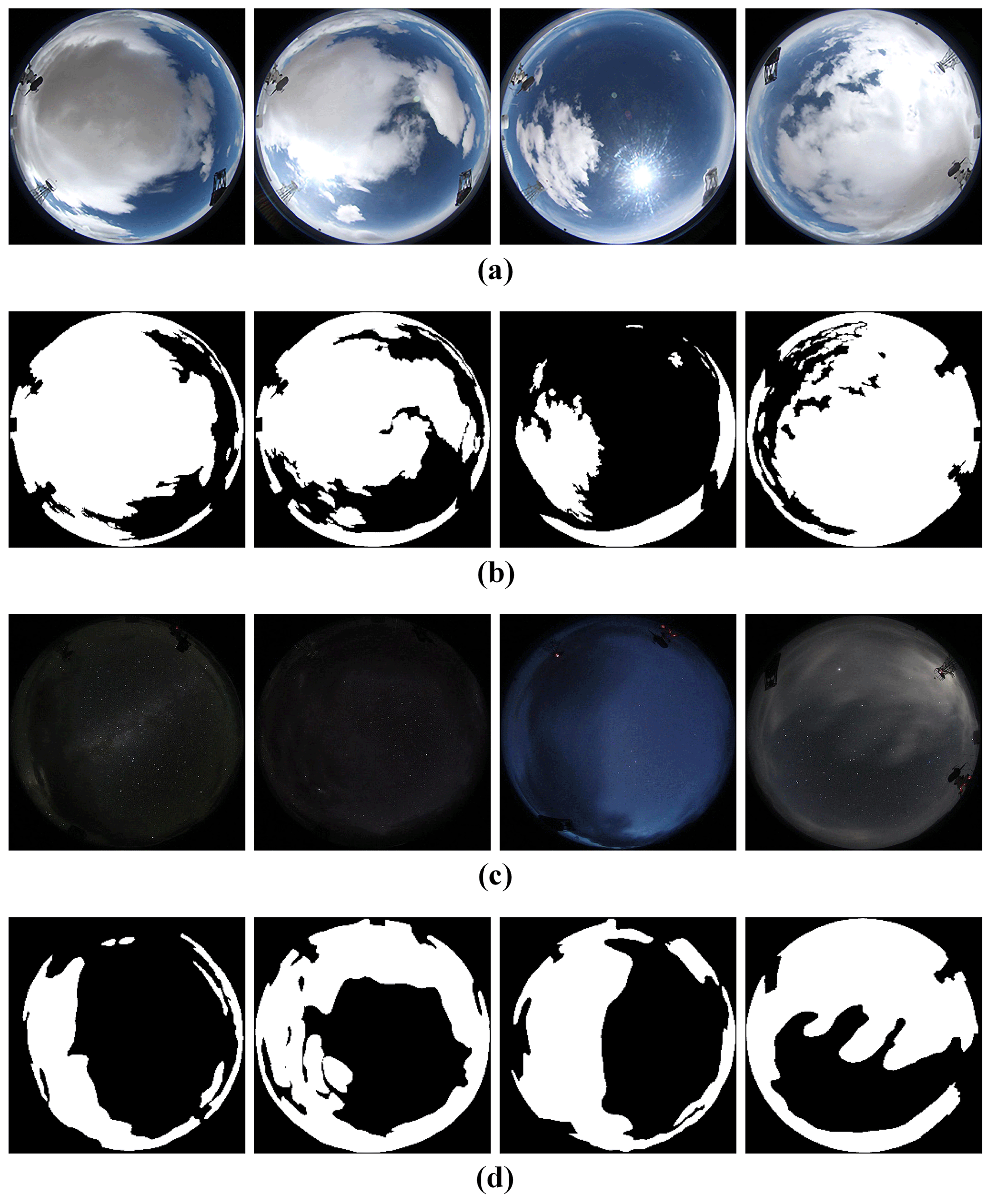
Figure 2Diurnal and nocturnal original RGB color ASI images in the data set and the corresponding ground truth of the ASI images. (a) Diurnal original RGB color ASI images in the data set, (b) corresponding ground truth ASI images from (a), (c) nocturnal original RGB color ASI images in the data set, and (d) corresponding ground truth of ASI images from (c).
This section describes the proposed EFCN, which utilizes the deep-learning algorithm FCN to segment cloud pixels from diurnal and nocturnal ASI images. Firstly, we sketch the proposed EFCN, and then the details of the EFCN are described.
3.1 Sketch on EFCN for ASI image segmentation
The proposed EFCN is an improvement of FCN. Firstly, the resized ASI images in the data set are converted from the RGB color space to the HSI color space (RGB–HSI). Secondly, the I channel is separated from HSI color space. The I channel is then equalized by histogram equalization in order to enhance the intensity and maintain a constant saturation and hue of the resized ASI images. Thirdly, the ASI images in the data set are converted from the HSI color space back to the RGB color space (HSI–RGB), and we use the training set to train the EFCN model. The associated parameters are obtained. Finally, the test set is input to the trained model to segment cloud pixels in the ASI images and assess the performance of the model. The different steps will be explained in the following subsections.
3.2 EFCN
Fully convolutional networks are a powerful visual deep-learning algorithm for semantic segmentation (Shelhamer et al., 2017). By replacing the fully connected layers of traditional convolutional neural networks (CNNs) with convolutional layers, the FCN reduces the number of network parameters, improves the segmentation speed, and shows a good result on semantic segmentation through training end to end and pixel to pixel (Cheng and Lin, 2017). The basic components of FCN include convolutional layers, pooling layers, activation functions, and deconvolutional layers, as shown in Fig. 3. At present, FCNs are widely used in medical image processing, remote sensing image processing, computer vision, and other fields (Yuan et al., 2017; Jiao et al., 2017; Lopez-Linares et al., 2018; Zeng and Zhu, 2018).
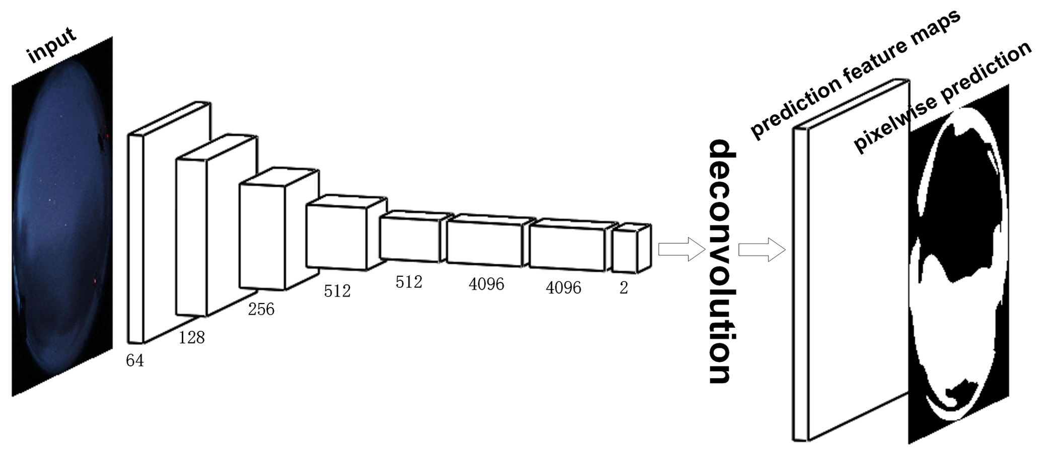
Figure 3Basic components of FCN model including convolutional layers, pooling layers, activation functions, and deconvolutional layers.
However, the FCN has some disadvantages in segmenting cloud pixels in diurnal and nocturnal ASI images. Therefore, the EFCN is proposed based on the VGG-16 network to replace the fully connected layer of VGG-16 with a convolutional layer and outputs an up-sampled prediction. Enhancement fully convolutional networks can accept input diurnal and nocturnal ASI images in any size, producing a prediction for each pixel, with the output of the prediction being the same size as the input ASI image. Unlike CNN, the EFCN can classify ASI images at the pixel level. Figure 4 illustrates the detailed architecture of the EFCN model, including the RGB–HSI layer, histogram equalization layer, HSI–RGB layer, convolutional layers, pooling layers, deconvolutional layers, skip architecture, and activation functions.
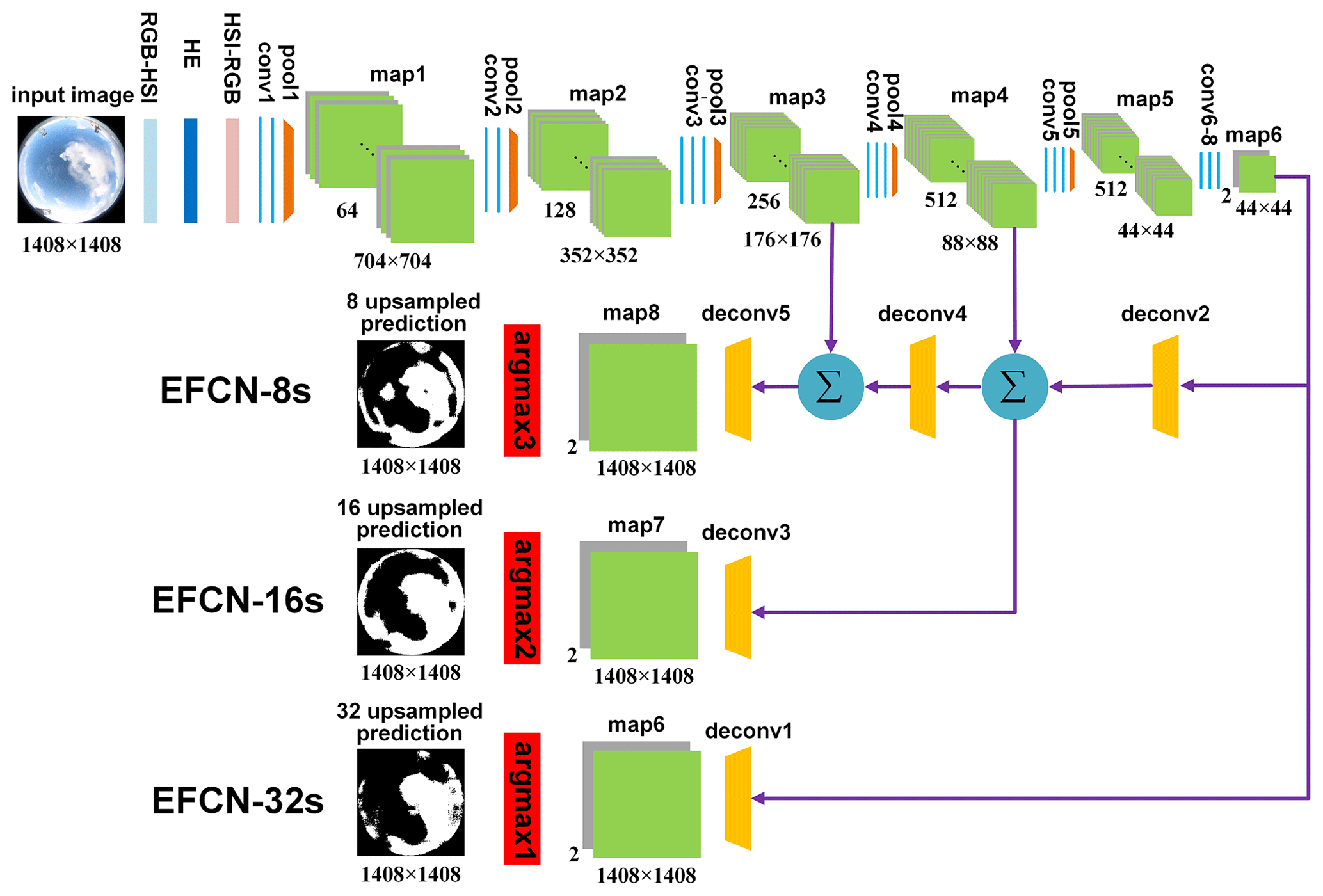
Figure 4Detailed architecture of EFCN model including RGB–HSI layer, histogram equalization layer, HSI–RGB layer, convolutional layers, pooling layers, deconvolutional layers, skip connection, and activation functions.
Images from an all-sky imager are usually not very clear due to complex weather conditions, especially at night. We need to use an image enhancement method to process the ASI images for better features and visual effects. Using histogram equalization to equalize any channel of the RGB color space can cause a change in the hue and saturation of ASI images. However, the ASI images are enhanced in the I channel of HSI color space, and the hue and saturation channels remain constant. We convert the ASI images from the RGB to HSI color space and use histogram equalization to equalize the I channel of the HSI color space. Then the images are converted from the HSI back to RGB color space to obtain the enhanced images. This method is stable and fast. The EFCN model in Fig. 4 has eight convolutional layers. The number of convolution kernels is different for each convolutional layer. We define the size and stride of the convolutional kernel. Each convolutional kernel has the same size and stride. The size is 3×3 and the stride is 1. The role of the convolutional layer is to extract features from images, and different convolutional layers can extract different features. In order to ensure that the size of the feature map after convolution is consistent with the size before convolution, we use a zero pad operation. The convolution calculation formula can be expressed as follows:
where l represents the number of layers in the neural network, v represents feature maps, n represents convolutional kernels, bC represents the bias of output feature maps, Nv represents the collection of input feature maps, and f represents an activation function. This paper adopts the rectified linear unit (ReLU) as an activation function. The ReLU activation function is defined as follows:
where l represents the number of layers in the neural network, and v represents feature maps. A pooling operation is a down-sampling process. The pooling layer is located after the convolution layer, which can further extract features, reduce the size of the feature maps, speed up calculations, and prevent overfitting. This paper uses the max-pooling method. Through the max-pooling operation, the size of the feature maps is reduced by half. After eight convolution operations and five pooling operations as shown in Fig. 4, the resolution of the input ASI image is reduced by 2, 4, 8, 16, and 32 times. Meanwhile, we get two heat maps as shown in map6 in Fig. 4. Heat maps are one of the most important high-dimensional feature maps. Our goal is to separate the cloud from the sky background, so we need to get two heat maps. Following that, a very important step is to up-sample the heat maps so that the two heat maps in map6 are enlarged to the same size as the input ASI image.
We use a deconvolution operation to up-sample the two heat maps in map6 that are output from the last convolutional layer, enlarge them by 32 times, and return them to the same size as the input ASI image, while retaining the spatial information in the original input image so that we can generate and predict each pixel. Finally, we use the argmax1 function to classify each pixel. The pixel classification is determined by the maximum value of the corresponding pixel positions of the two heat maps in map7. We get the 32 up-sample prediction and refer to this model as EFCN-32s. However, EFCN-32s is too rough to restore the features in the input image well. The segmentation result is not very accurate, and some details cannot be restored. Therefore, we propose a skip connection structure. The heat maps in map6 are up-sampled by a factor of 2 through the deconv2 layer and then integrated with the feature maps in map4. The integrated feature maps are up-sampled by a factor of 16 through the deconv3 layer to obtain the feature maps of the same size as the input ASI image. We get the 16 up-sample prediction after the argmax2 function and refer to this model as EFCN-16s. The integrated feature maps are up-sampled by a factor of 2 through the deconv4 layer and then integrated with the feature maps in map3. The second integrated feature maps are up-sampled by a factor of 8 through the deconv5 layer to obtain feature maps of the same size as the input ASI image. We get the 8 up-sample prediction after the argmax3 function and refer to this model as EFCN-8s.
Table 1Detailed parameters of the proposed EFCN-8s for segmenting cloud pixels from ASI images.
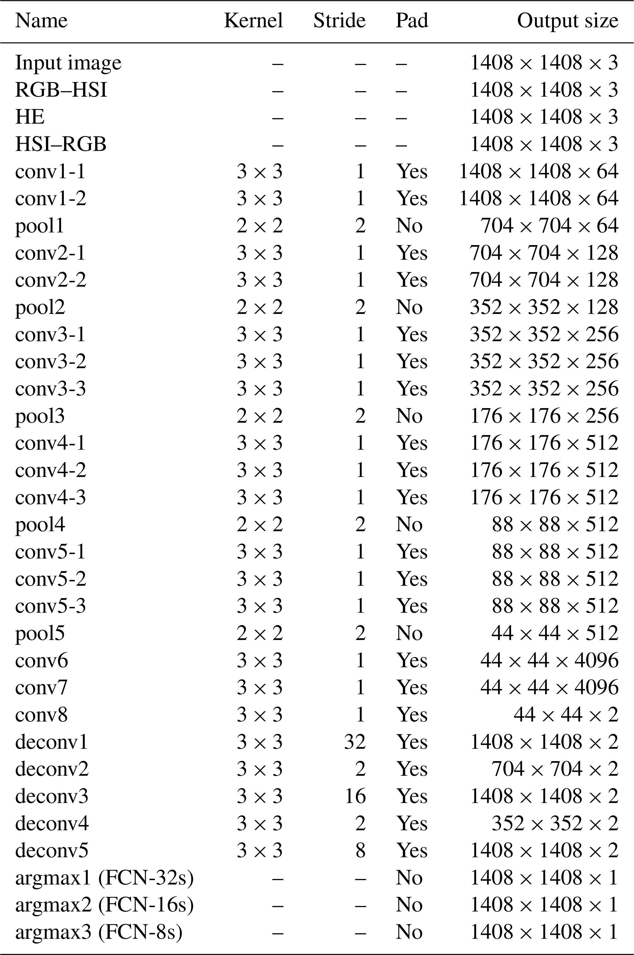
Table 1 summarizes the parameters of the proposed EFCN, which are shown in Fig. 4. Here “HE” represents histogram equalization, “conv” represents the convolution operation, “pool” represents the max-pooling operation, and “deconv” represents the deconvolution operation. The up-sampled prediction is the same size as the input ASI image.
The complete proposed automatic cloud segmentation based on EFCN-8s is summarized as follows in Algorithm 1.
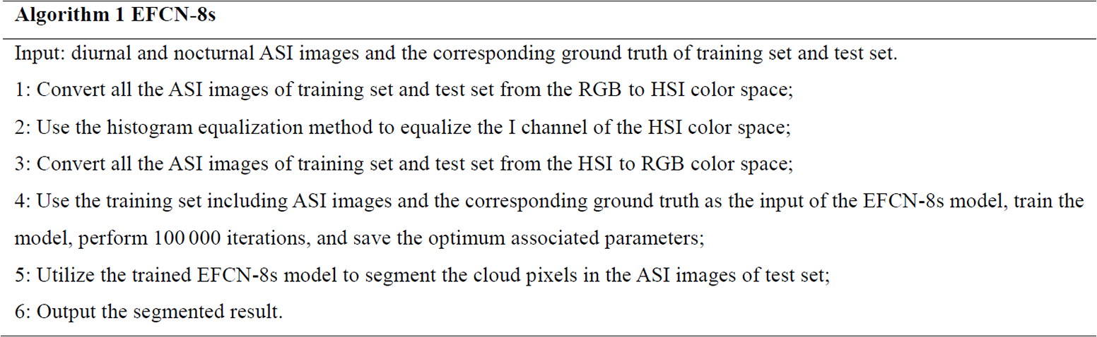
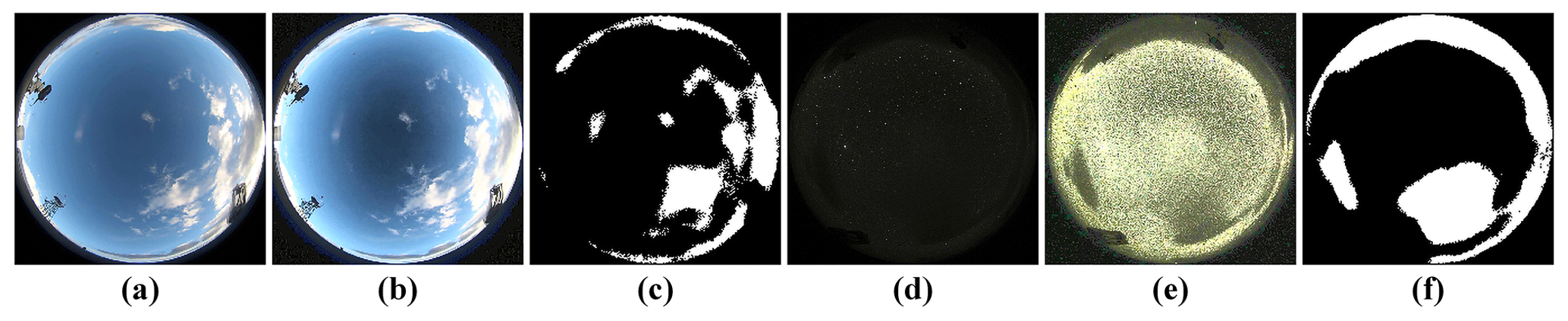
Figure 5Framework of the complete proposed automatic cloud segmentation based on EFCN-8s. (a) Original diurnal ASI image from the test set, which is the input test image of the EFCN-8s. (b) Enhanced diurnal ASI image using the histogram equalization, (c) diurnal cloud segmentation result using the trained EFCN-8s, (d) original nocturnal ASI image from the test set, which is the input test image of the EFCN-8s, (e) enhanced nocturnal ASI image using the histogram equalization, and (f) nocturnal cloud segmentation result using the trained EFCN-8s.
We illustrate the framework of the proposed automatic cloud segmentation algorithm based on EFCN-8s in Fig. 5. Figure 5a presents the input test ASI image of the EFCN-8s model captured in daytime, which is enhanced by the method of histogram equalization as shown in Fig. 5b. Figure 5c presents the cloud segmentation result using the trained EFCN-8s model. Figure 5d presents the input test ASI image of the EFCN-8s model captured at night, which is enhanced by the method of histogram equalization as shown in Fig. 5e. Figure 5f presents the cloud segmentation result using the trained EFCN-8s model.
We design three sets of experiments to segment the cloud pixels from the resized diurnal and nocturnal ASI images and analyze the experimental results in detail based on four evaluation metrics.
4.1 Experiments
We randomly select 1124 ASI images as our data set, including 369 diurnal ASI images and 755 nocturnal ASI images. We use the software LabelMe to label these ASI images. The 1054 ASI images and the corresponding labels are randomly selected as the training set, including 343 diurnal images and 711 nocturnal images. Another 70 ASI images and corresponding labels are used as a test set, including 26 diurnal ASI images and 44 nocturnal ASI images. The training set is iteratively trained on the EFCN-8s model, which is iterated 100 000 times, and the best model parameters are obtained. The data from the test set are used to verify the robustness and accuracy of EFCN-8s. We design three sets of experiments to segment cloud pixels from the ASI images. In the first set of experiments, the cloud pixels are segmented in the diurnal ASI images. In the second set of experiments, the cloud pixels are segmented in the nocturnal ASI images. In the third set of experiments, the cloud pixels are segmented in the diurnal and nocturnal ASI images.
In the first set of experiments, we used the proposed EFCN-8s, EFCN-16s, EFCN-32s, FCN-8s, and OTSU algorithms to segment cloud pixels in the diurnal ASI images. The OTSU algorithm is a classic automatic threshold selection algorithm for image segmentation without parameters or supervision (Otsu, 1979). This algorithm is one of the most commonly used image segmentation algorithms with a discriminant to determine the optimal threshold without any prior information. The cloud segmentation results are shown in Fig. 6. Figure 6a presents the resized diurnal ASI images, and Fig. 6b shows the enhanced diurnal ASI images. Figure 6c denotes the ground truth of the corresponding ASI images. The results of cloud segmentation by OTSU, FCN-8s, EFCN-32s, EFCN-16s, and EFCN-8s are shown in Fig. 6d–h, respectively.
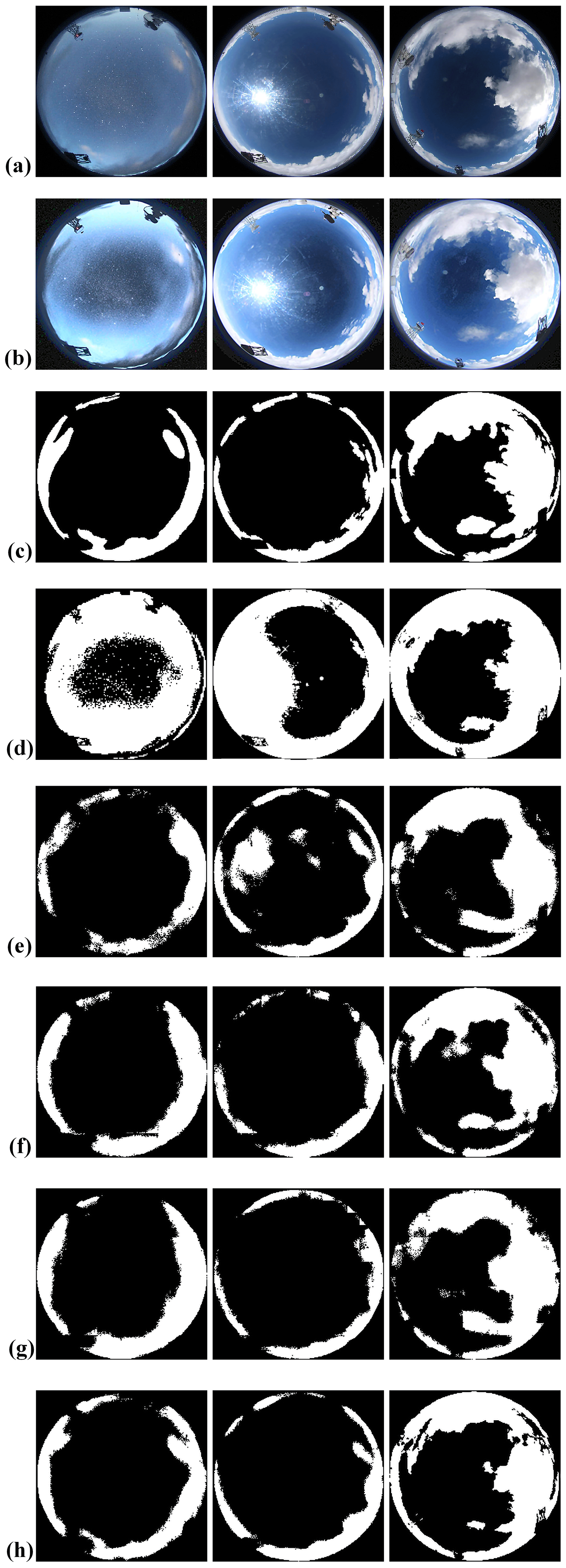
Figure 6Results of different cloud segmentation algorithms. (a) Original diurnal ASI images, (b) enhanced diurnal ASI images, (c) ground truth of the corresponding ASI images in (a), (d) results of OTSU, (e) results of EFCN-32s, (f) results of EFCN-16s, (g) results of FCN-8s, and (h) results of the proposed EFCN-8s.
As shown in Fig. 6, the OTSU has good cloud segmentation accuracy under a clear-sky background without sunlight. However, the segmentation accuracy is poor when sunlight is visible in the images or the brightness of the images is low. For the EFCN-32s, the recognition accuracy is improved compared with the OTSU algorithm. The EFCN-16s segments cloud better than EFCN-32s, but the details of cloud are not recognized. In addition to the diurnal ASI images with visible sun, the segmentation performance of the FCN-8s is usually good. The recognition accuracy of the EFCN-8s is very good for almost all the diurnal ASI images. The details of the cloud can be identified without the influence of sunlight.
In the second set of experiments, we used the proposed EFCN-8s to segment cloud pixels in the nocturnal ASI images and compared the result with the EFCN-16s, EFCN-32s, FCN-8s, and OTSU algorithms. The different experimental segmentation results are shown in Fig. 7. Figure 7a presents the resized nocturnal ASI images, and Fig. 7b shows the enhanced nocturnal ASI images. Figure 7c denotes the ground truth of the corresponding ASI images. The different results of cloud segmentation are shown in Fig. 7d–h.
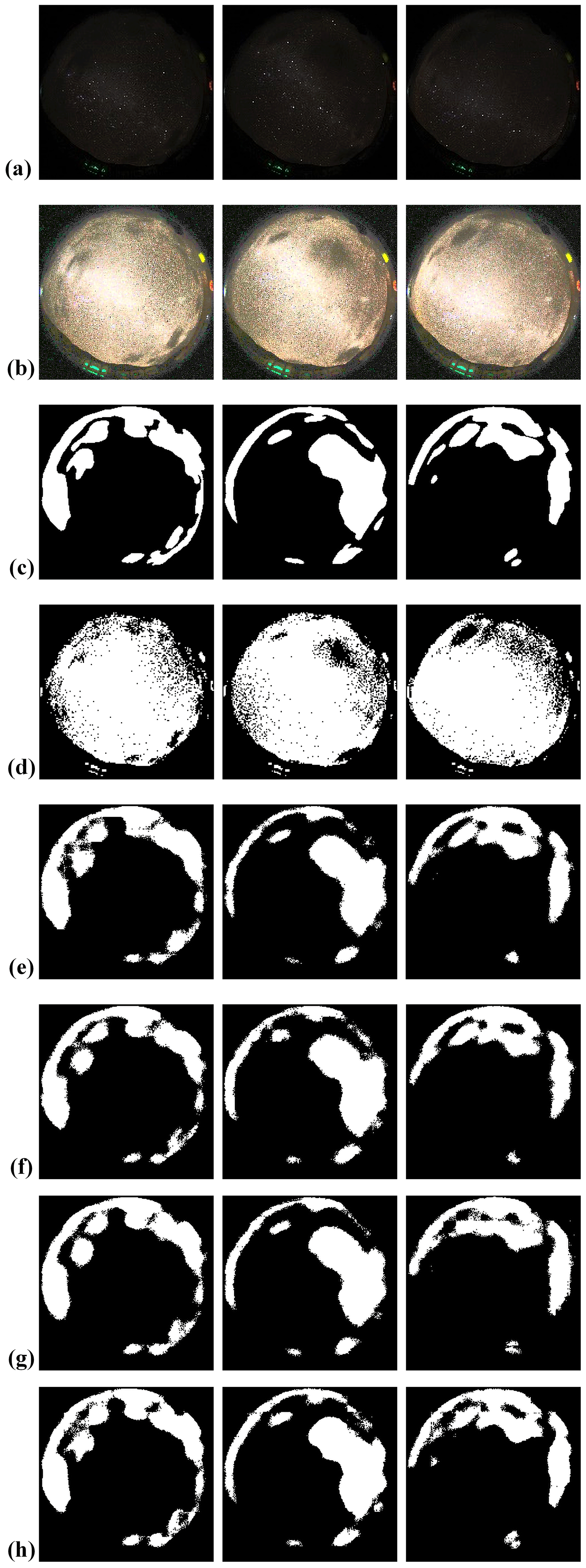
Figure 7Results of different cloud segmentation algorithms. (a) Original nocturnal ASI images, (b) enhanced nocturnal ASI images, (c) ground truth of the corresponding ASI images in (a), (d) results of OTSU, (e) results of EFCN-32s, (f) results of EFCN-16s, (g) results of FCN-8s, and (h) results of the proposed EFCN-8s.
As shown in Fig. 7, the proposed EFCN-8s shows the best segmentation results. The results of EFCN-32s, EFCN-16s, and FCN-8s are better, and the segmentation results are close. However, the details of cloud are not recognized. The experimental results using OTSU are very poor. Most of the sky background pixels are mistakenly segmented into cloud pixels.
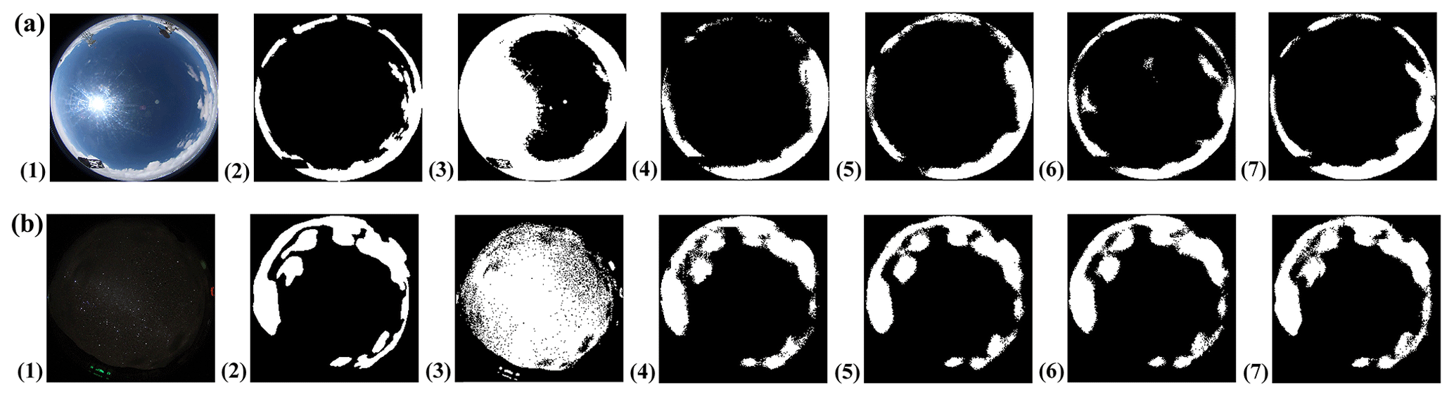
Figure 8Results of different diurnal and nocturnal cloud segmentation algorithms. (a) Results of different diurnal cloud segmentation algorithms. (b) Results of different nocturnal cloud segmentation algorithms. (a1) Original diurnal ASI image, (a2) ground truth of the corresponding ASI image in (a1), (b1) original nocturnal ASI image, (b2) ground truth of the corresponding ASI image in (b1), (a3), (b3) results of OTSU, (a4), (b4) results of EFCN-32s, (a5), (b5) results of EFCN-16s, (a6), (b6) results of FCN-8s, and (a7), (b7) results of the proposed EFCN-8s.
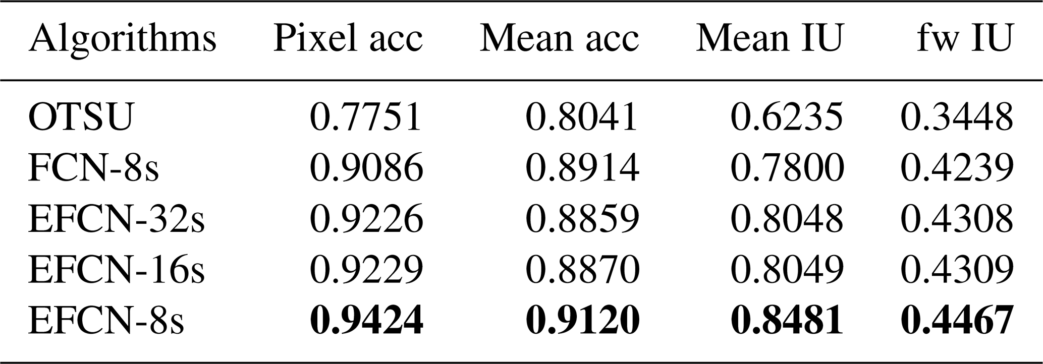
Table 2Comparison of cloud segmentation results of different algorithms on diurnal ASI images. The enhanced performance values are highlighted in bold font.
In the third set of experiments, the cloud pixels in the diurnal and nocturnal ASI images are segmented simultaneously. The segmentation results of the proposed EFCN-8s and the other four algorithms are shown in Fig. 8. Figure 8a presents the diurnal ASI image, the ground truth of the corresponding ASI image, and the segmentation results of the proposed EFCN-8s and the other four algorithms. Figure 8b presents the nocturnal ASI image, the ground truth of the corresponding ASI image, and the segmentation results of the proposed EFCN-8s and the other four algorithms. As shown in Fig. 8, consistent with the results obtained in experiment 1 and experiment 2, the proposed EFCN-8s has the best segmentation results, which verifies that the proposed algorithm is robust.
4.2 Evaluation metrics
In order to better evaluate the results of the experiments, we adopt four effective evaluation metrics to analyze the experimental results, which covered pixel accuracy and region intersection over union (IU) (Shelhamer et al., 2017). The four effective evaluation metrics, including pixel accuracy (pixel acc), mean accuracy (mean acc), mean IU, and frequency-weighted IU (fw IU), are defined as follows.
Pixel accuracy (pixel acc), mean accuracy (mean acc), frequency-weighted IU (fw IU), mean IU, and k indicate that each ASI image in the test set can be segmented into the k class, including clouds and sky background; pij represents the number of pixels of class i predicted to class j. Among the above four metrics, mean IU is the most commonly used metric because it is simple and representative.
4.3 Experimental results comparison
To better demonstrate the performance of the proposed EFCN-8s, we adopt four evaluation metrics defined in the previous section to compare the segmentation results with other algorithms including OTSU, FCN-8s, EFCN-32s, and EFCN-16s.
Table 2 lists the performance of different algorithms on the cloud segmentation of diurnal ASI images in the first set of experiments. From Table 2, we have the following observations. Firstly, the mean IU in the traditional OTSU result is 0.6235. The mean IU of the deep-learning algorithm FCN-8s is raised by 0.1565 to 0.7800. The EFCN-32s based on VGG-16 increased the mean IU by 0.8048. The EFCN-16s adds the skip connection structure that integrates the features of map6 and map5, resulting in a mean IU of 0.8049. The proposed EFCN-8s integrates the features of map6, map5, and map4, achieving a significant improvement to a mean IU of 0.8481. Secondly, the skip connection structure and image enhancement can improve the accuracy of segmentation. Moreover, we find that the proposed algorithm works better for diurnal ASI image segmentation.
Table 3 lists the performance of different algorithms on the cloud segmentation of nocturnal ASI images in the second set of experiments. For nocturnal ASI images, the proposed EFCN-8s demonstrates strong advantages. When compared with other algorithms, it shows an increase of 0.1673 in pixel acc compared with OTSU, an increase of 0.0206 in mean acc compared with FCN-8s, an increase of 0.0433 in mean IU compared with EFCN-32s, and an increase of 0.0158 in fw IU compared with EFCN-16s.
Table 3Comparison of cloud segmentation results of different algorithms on nocturnal ASI images. The enhanced performance values are highlighted in bold font.
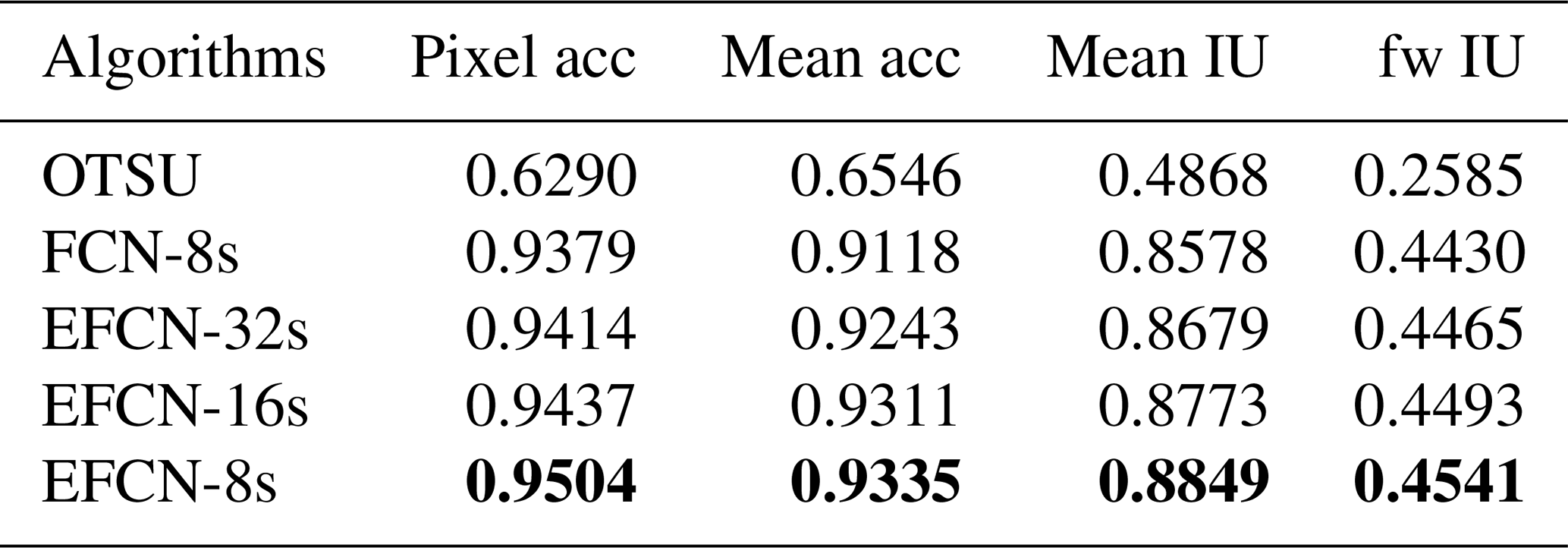
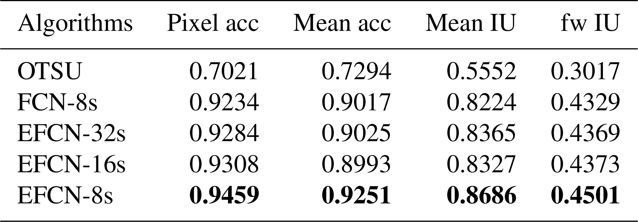
Table 4Comparison of cloud segmentation results of different algorithms on diurnal and nocturnal ASI images. The enhanced performance values are highlighted in bold font.
Comparing Tables 2 and 3, we can get the following observations. Firstly, the traditional threshold algorithm OTSU has a better segmentation result on diurnal ASI images than nocturnal ASI images. Secondly, the deep-learning algorithms FCN-8s, EFCN-32s, EFCN-16s, and EFCN-8s can extract the deep features of the ASI images and integrate multiple features. At the same time, due to the influence of sunlight, the nocturnal ASI image segmentation results are better than the diurnal ASI images.
Table 4 lists the performance of different algorithms on the cloud segmentation of diurnal and nocturnal ASI images in the third set of experiments. Table 4 shows that the results obtained in the third set of experiments are consistent with the first and second set of experiments. The proposed EFCN-8s has the best segmentation results compared with the other four algorithms (OTSU, FCN-8s, EFCN-32s, and EFCN-16s). The mean IU of the proposed EFCN-8s in experiment 3 increases by 0.0205 compared with experiment 1 and decreases by 0.0163 compared with experiment 2. This result verifies that the proposed EFCN-8s is robust.
Cloud segmentation is a huge challenge for astronomical researchers today. This paper proposed a new automatic cloud segmentation algorithm, EFCN-8s, to segment cloud pixels from diurnal and nocturnal ASI images. The cloud images were taken by the ASI provided by the Key Laboratory of Optical Astronomy at the National Astronomical Observatories of CAS. We used the software LabelMe to semantically label the ASI images and created the ground truth. The proposed EFCN-8s was based on the VGG-16 net. Histogram equalization enhances the intensity of the images, and the skip connection integrated the different features of the image together. The two operations, including histogram equalization and the skip connection, were applied to increase the segmentation performance.
To verify the performance of the proposed algorithm, we designed three sets of experiments. In the first set of experiments, the proposed EFCN-8s was used to segment the diurnal ASI images. It reduced the influence of the sun and a good segmentation result was obtained on the test set. In the second set of experiments, the EFCN-8s extracted multidimensional features for nighttime ASI images and also had good segmentation results. In the third set of experiments, the cloud pixels in the diurnal and nocturnal ASI images were segmented simultaneously. The results were consistent with the first and second set of experiments, which verified that the proposed EFCN-8s was robust. After that, the EFCN-8s was compared with four other algorithms including OUSU, FCN-8s, EFCN-32s, and EFCN-16s. To better verify the performance, we adopted four evaluation metrics to measure the segmentation results. The results show that the EFCN-8s is much more accurate at cloud segmentation for diurnal and nocturnal ASI images than the other four algorithms.
It should be noted that the EFCN-8s still has some limitations. Firstly, it can be seen from Tables 1 and 2 that the EFCN-8s is better than diurnal ASI images for nocturnal ASI image segmentation. This may be due to interference from the sun. Secondly, since the ground truth of the data set is manually labeled by us, it has some errors for the true values of cloud. In future work, we will remove the interference of the sun first and use a more advanced approach to label the data sets.
The data are provided by the National Astronomical Observatories, Chinese Academy of Sciences, (NAO-CAS) and we need to apply to the NAO-CAS before we publish the data set. The data will be made available from author Chaojun shi (474756323@qq.com) and corresponding author Yatong Zhou (zyt@hebut.edu.cn) upon request.
CS, YZ, and BQ conceived and designed the experiments; CS performed the experiments, drafted, and revised the manuscript; YZ and JH proposed constructive suggestions on the revision of the manuscript; MD created the ground truth of the data set using LabelMe; SW collected relevant literature.
The authors declare that they have no conflict of interest.
We would like to thank the National Astronomical Observatories, Chinese Academy of Sciences, for providing us with the original cloud images. Moreover, we would like to thank the referees for their comments and Murray Hamilton for handling the paper.
This research has been supported by the National Natural Science Foundation of China (grant no. 61801164), the Tianjin Natural Science Foundation (grant no. 18JCQNJC01700), and the Hebei Province Foundation of Returned Oversea Scholars (grant no. CL201707).
This paper was edited by Murray Hamilton and reviewed by two anonymous referees.
Aebi, C., Gröbner, J., and Kämpfer, N.: Cloud fraction determined by thermal infrared and visible all-sky cameras, Atmos. Meas. Tech., 11, 5549–5563, https://doi.org/10.5194/amt-11-5549-2018, 2018.
Calbo, J. and Sabburg, J.: Feature extraction from whole-sky ground-based images for cloud-type recognition, J. Atmos. Ocean. Tech., 25, 3–14, https://doi.org/10.1175/2007JTECHA959.1, 2008.
Calbo, J., Long, C. N., Gonzalez, J. A., Augustine, J., and McComiskey, A.: The thin border between cloud and aerosol: Sensitivity of several ground based observation techniques, Atmos. Res., 196, 248–260, https://doi.org/10.1016/j.atm osres.2017.06.010, 2017.
Cazorla, A., Olmo, F. J., and Alados-Arboledasl, L.: Development of a sky imager for cloud cover assessment, J. Opt. Soc. Am. A., 25, 29–39, https://doi.org/10.1364/JOSAA.25.000029, 2008.
Cheng, H.-Y. and Lin, C.-L.: Cloud detection in all-sky images via multi-scale neighborhood features and multiple supervised learning techniques, Atmos. Meas. Tech., 10, 199–208, https://doi.org/10.5194/amt-10-199-2017, 2017.
Dev, S., Lee, Y. H., and Winkler, S.: Color-based segmentation of sky/cloud images from ground-based cameras, IEEE J. Sel. Top. Appl., 10, 231–242, https://doi.org/10.1109/JSTARS.2016.2558474, 2017a.
Dev, S., Savoy, F. M., Lee, Y. H., and Winkler, S.: Nighttime sky/cloud image segmentation, 2017 IEEE International Conference on Image Processing, https://doi.org/10.1109/ICIP.2017.8296300, 2017b.
Dev, S., Nautiyal, A., Lee, Y. H., and Winkler, S.: CloudSegNet: A Deep Network for Nychthemeron Cloud Image Segmentation, IEEE Geosci. Remote S., https://doi.org/10.1109/LGRS.2019.2912140, 2019.
Gacal, G. F. B., Antioquia, C., and Lagrosas, N.: Ground-based detection of nighttime clouds above Manila Observatory (14.64 degrees N, 121.07 degrees E) using a digital camera, Appl. Optics, 55, 6040–6045, https://doi.org/10.1364/AO.55.006040, 2016.
Ghonima, M. S., Urquhart, B., Chow, C. W., Shields, J. E., Cazorla, A., and Kleissl, J.: A method for cloud detection and opacity classification based on ground based sky imagery, Atmos. Meas. Tech., 5, 2881–2892, https://doi.org/10.5194/amt-5-2881-2012, 2012.
Heinle, A., Macke, A., and Srivastav, A.: Automatic cloud classification of whole sky images, Atmos. Meas. Tech., 3, 557–567, https://doi.org/10.5194/amt-3-557-2010, 2010.
Hinton, G. E. and Salakhutdinov, R. R.: Reducing the dimensionality of data with neural networks, Science, 313, 504–507, https://doi.org/10.1126/science.1127647, 2006.
Jiao, L. C., Liang, M. M., Chen, H., Yang, S., Y., Liu, H. Y., and Cao, X. H.: Deep fully convolutional network-based spatial distribution prediction for hyperspectral image classification, IEEE T. Geosci. Remote, 55, 5585–5599, https://doi.org/10.1109/TGRS.2017.2710079, 2017.
Johnson, R.W., Hering, W. S., and Shields, J. E.: Automated visibility and cloud cover measurements with a solid-state imaging system, University of California, San Diego, Scripps Institution of Oceanography, Marine Physical Laboratory, SIO89-7, GL-TR-89-0061, 1989.
Klebe, D. I., Blatherwick, R. D., and Morris, V. R.: Ground-based all-sky mid-infrared and visible imagery for purposes of characterizing cloud properties, Atmos. Meas. Tech., 7, 637–645, https://doi.org/10.5194/amt-7-637-2014, 2014.
Krizhevsky, A., Sutskever, I., and Hinton, G. E.: Imagenet classification with deep convolutional neural networks, Commun. ACM, 60, 84–90, https://doi.org/10.1145/3065386, 2017.
Kuji, M., Murasaki, A., Hori, M., and Shiobara, M.: Cloud fractions estimated from shipboard whole-sky camera and ceilometer observations between east Asia and Antarctica, J. Meteorol. Soc. Jpn., 96, 201–214, https://doi.org/10.2151/jmsj.2 018-025, 2018.
LeCun, Y., Boser, B., Denker, J. S., Henderson, D., Howard, R. E., Hubbard, W., and Jackel, L. D.: Backpropagation applied to handwritten zip code recognition, Neural Comput., 11, 541–551, https://doi.org/10.1162/neco.1989.1.4.541,1989.
Li, Q. Y., Lu, W. T., and Yang, J.: A hybrid thresholding algorithm for cloud detection on ground-based color images, J. Atmos. Ocean. Tech., 28, 1286–1296, https://doi.org/10.1175/JTECH-D-11-00009.1, 2011.
Long, C. N. and Deluisi, J. J.: Development of an automated hemispheric sky imager for cloud fraction retrievals, in: Proc. 10th Symp. on meteorological observations and instrumentation, 11–16 January 1998, Phoenix, Arizona, USA, 171–174, 1998.
Long, C. N., Sabburg, J. M., Calbo, J., and Pages, D.: Retrieving cloud characteristics from ground-based daytime color all-sky images, J. Atmos. Ocean. Tech., 23, 633–652, https://doi.org/10.1175/JTECH1875.1, 2006.
Lopez-Linares, K., Aranjuelo, N., Kabongo, L., Maclair, G., Lete, N., Ceresa, M., Garcia-Familiar, A., Macia, I., and Ballester, M. A. G.: Fully automatic detection and segmentation of abdominal aortic thrombus in post-operative CTA images using deep convolutional neural networks, Med. Image Anal., 46, 203–214, https://doi.org/10.1016/j.media.2018.03.010, 2018.
Neto, S. L. M., von Wangenheim, A., Pereira, E. B., and Comunello, E.: The use of euclidean geometric distance on rgb color space for the classification of sky and cloud patterns, J. Atmos. Ocean. Tech., 27, 1504–1517, https://doi.org/10.1175/2010JTECHA1353.1, 2010.
Ning, F., Delhomme, D., LeCun, Y., Piano, F., Bottou, L., and Barbano, P. E., Toward automatic phenotyping of developing embryos from videos, IEEE T. Image Process., 14, 1360–1371, https://doi.org/10.1109/TIP.2005.852470, 2005.
Nugent, P. W., Shaw, J. A., and Piazzolla, S.: Infrared cloud imaging in support of Earth-space optical communication, Opt. Express, 17, 7862–7872, https://doi.org/10.1364/OE.17.007862, 2009.
Nugent, P. W., Shaw, J. A., and Pust, N. J.: Correcting for focal-plane-array temperature dependence in microbolometer infrared cameras lacking thermal stabilization, Opt. Eng., 52, 061304, https://doi.org/10.1117/1.OE.52.6.061304, 2013.
Otsu, N.: A Threshold Selection Method from Gray-Level Histograms, IEEE T. Syst. Man Cyb., 9, 62–66, https://doi.org/10.1109/TSMC.1979.4310076, 1979.
Peng, Z. Z., Yu, D. T., Huang, D., Heiser, J., Yoo, S., and Kalb, P.: 3D cloud detection and tracking system for solar forecast using multiple sky imagers, Sol. Energy, 118, 496–519, https://doi.org/10.1016/j.solener.2015.05.037, 2015.
Roman, R., Cazorla, A., Toledano, C., Olmo, F. J., Cachorro, V. E., de Frutos, A., and Alados-Arboledas, L.: Cloud cover detection combining high dynamic range sky images and ceilometer measurements, Atmos. Res., 196, 224–236, https://doi.org/10.1016/j.atmosres.2017.06.006, 2017.
Shaw, J. A., Nugent, P. W., Pust, N. J., Thurairajah, b., and Mizutani, K.: Radiometric cloud imaging with an uncooled microbolometer thermal infrared camera, Opt. Express, 13, 5807–5817, https://doi.org/10.1364/OPEX.13.005807, 2005.
Shelhamer, E., Long, J., and Darrell, T.: Fully convolutional networks for semantic segmentation, IEEE T. Pattern. Anal., 39, 640–651, https://doi.org/10.1109/TPAMI.2016.2572683, 2017.
Shi, C. Z., Wang, Y., Wang, C. H., and Xiao, B. H.: Ground-based cloud detection using graph model built upon superpixels, IEEE Geosci. Remote S., 14, 719–723, https://doi.org/10.1109/LGRS.2017.2676007, 2017.
Souza-Echer, M. P., Pereir-A, E. B., Bins, L. S., and Andrade, M.A.R.: A simple method for the assessment of the cloud cover state in high-latitude regions by a ground-based digital camera, J. Atmos. Ocean. Tech., 23, 437–447, https://doi.org/10.1175/JTECH1833.1, 2006.
Stephens, G. L.: Cloud feedbacks in the climate system: a critical review, J. Climate, 18, 237–273, https://doi.org/10.1175/JCLI-3243.1, 2005.
Sun, X. J., Gao, T. C., Zhai, D. L., Zhao, S. J., and Lian, J. G.: Whole sky infrared cloud measuring system based on the uncooled infrared focal plane array, Infrared and Laser Engineering, 37, 761–764, 2008.
Tapakis, R. and Charalambides, A. G.: Equipment and methodologies for cloud detection and classification: a review, Sol. Energy, 95, 392–430, https://doi.org/10.1016/j.solener.2012.11.015, 2013.
Thurairajah, B. and Shaw, J. A.: Cloud statistics measured with the infrared cloud imager (ICI), IEEE T. Geosci. Remote, 43, 2000–2007, https://doi.org/10.1109/TGRS.2005.853716, 2005.
Yang, J., Lu, W., Ma, Y., and Yao, W.: An automated cirrus cloud detection method for a ground-based cloud image, J. Atmos. Ocean. Tech., 29, 527–537, https://doi.org/10.1175/JTECH-D-11-00002.1, 2012.
Yang, J., Min, Q., Lu, W., Yao, W., Ma, Y., Du, J., Lu, T., and Liu, G.: An automated cloud detection method based on the green channel of total-sky visible images, Atmos. Meas. Tech., 8, 4671–4679, https://doi.org/10.5194/amt-8-4671-2015, 2015.
Yang, J., Min, Q., Lu, W., Ma, Y., Yao, W., Lu, T., Du, J., and Liu, G.: A total sky cloud detection method using real clear sky background, Atmos. Meas. Tech., 9, 587–597, https://doi.org/10.5194/amt-9-587-2016, 2016.
Yang, J., Min, Q., Lu, W., Ma, Y., Yao, W., and Lu, T.: An RGB channel operation for removal of the difference of atmospheric scattering and its application on total sky cloud detection, Atmos. Meas. Tech., 10, 1191–1201, https://doi.org/10.5194/amt-10-1191-2017, 2017.
Yuan, Y. D., Chao, M., and Lo, Y. C.: Automatic skin lesion segmentation using deep fully convolutional networks with Jaccard distance, IEEE T. Med. Imaging, 36, 1876–1886, https://doi.org/10.1109/TMI.2017.2695227, 2017.
Zeng, D. D. and Zhu, M.: Background subtraction using multiscale fully convolutional network, IEEE Access, 6, 16010–16021, https://doi.org/10.1109/ACCESS.2018.2817129, 2018.