the Creative Commons Attribution 4.0 License.
the Creative Commons Attribution 4.0 License.
 | 05 Sep 2019
Derivation of flow rate and calibration method for high-volume air samplers
Mark Hermanson
Sampling the atmosphere to analyze contaminants is different from other environmental matrices because measuring the volume of air collected requires a mechanical flow-through device to draw the air and measure its flow rate. The device used must have the capability of concentrating the analytes of interest onto a different substrate because the volumes of air needed are often on the order of hundreds of cubic meters. The use of high-volume air samplers has grown since 1967, when recommended limits of a large number of organic contaminants in air were developed. Equations used for calculating the air flow through the device over time have similarly been developed. However, the complete derivation of those equations has never appeared in the scientific literature. Here a thorough derivation of those equations is provided with definitions of the mechanical systems that are used in the process, along with the method of calibrating and calculating air flow.


Collecting environmental samples of the atmosphere is inherently different from sampling soil, ice, snow, water, or organic matter. With the non-atmospheric matrices, the chemical analytes of interest are specific to a typically small and easily measured volume or mass. The atmosphere is a matrix with a significantly lower density, which raises the question of how to collect and measure the large volume of air where the analytes are found.
The first mention in the scientific literature of high-volume (Hi-Vol) air flow regulation was from a toxicological study by Drinker et al. (1937). In this study, the amount of chlorinated biphenyl released to specific amounts of air had to be known to identify the amount of toxic substance inhaled by the test organism. The air flow was measured by an orifice calibrator that enabled the volume of air to be known over a certain time period. Although the orifice calibrator is mentioned in this report, the calibration system, including the system of equations used for calculating flow, is not identified.
Following the passage of the US Clean Air Act in 1963, a group of US health experts formed a group known as the American Conference of Governmental Industrial Hygienists (ACGIH). In 1966, ACGIH developed recommended no-toxic-effect concentration limits in air of 78 different contaminants, many of them organic compounds (Danielson, 1967). The development of this list led to a requirement of making an air sampler capable of handling large volumes of air because the toxic amounts on the ACGIH list were very low and would be found in low concentrations. Development of Hi-Vol samplers began soon after, with early designs using vacuum systems that generated large flow rates (Jutze and Foster, 1967). After further development, these systems were found to provide reproducible results (Clements et al., 1972) and eventually to be reliable in severe weather (Salamova et al., 2014) and robust over many years when properly maintained (Salamova et al., 2016).
The early development of vacuum-assisted Hi-Vol samplers required a system for measuring the volume of air flow through the sampler. While Hi-Vol manufacturers and the literature now provide equations used for this process, none of them include any derivation of those calculations or discussion about why the variables in the equations are used. The situation is typical of a textbook by Wight (1994), where the basic fluid dynamic principles required for the calculations are outlined, but ultimately the equations are not derived comprehensively. Similarly, the coursework provided by the Air Pollution Training Institute on air sampling (APTI, 1980) presents only the calibration equations along with a multitude of numerical examples, without explaining their origin. Even governmental regulations (40 CFR Appendix B Part 50, US EPA, 2011) and guidelines (US EPA, 1999) focus on the calibration of Hi-Vol samplers but do not derive the procedure in detail. The early literature does not elaborate on the calibration equations. For example, Lynam et al. (1969) investigate different calibration methods for Hi-Vol samplers, showing that significant differences can occur. Similarly, Lee et al. (1972) investigate different methods for measuring suspended particles in air and elaborate in detail on the calibration process of Hi-Vol samplers without deriving any equations. As recently as 2013, ASTM International (2013), in Method D6209-13 for collection of Hi-Vol samples, leave several blanks in sections covering flow control, flow calibration, calibration orifices, and roots meters (Sect. 9.1.2, 9.1.3, 9.1.4 and 9.1.5), all of which are critical to proper calibration. In the calibration section of this method (12.1), there are references to these blanks in Sect. 9.1. Most studies of atmospheric contaminants collected with Hi-Vol samplers assume that the calibration procedure is understood, rarely discuss calibration details, and never include the equations used, this includes Hermanson and Hites (1989), Monosmith and Hermanson (1996), Hermanson et al. (1997, 2003, 2007), Basu et al. (2009), Salamova et al. (2014), and Hites (2018).
The objective here is to derive the calculations required for measurement of air flow, volume, and calibration of a Hi-Vol air sampler that are missing from the scientific literature. These calculations are based on principles of fluid dynamics. The results developed provide the air sampling community with the missing derivation of equations that are based on the physical features of a Hi-Vol system. The outcome will improve an air pollution investigator's understanding of the operational features of Hi-Vol samplers. Some specialty Hi-Vol samplers, including those for PM10, PM2.5, and total suspended particulates (TSPs) have different flow devices (e.g., particle pre-separators) or different metering systems, so the equations derived and conditions discussed here may not fully apply to them.
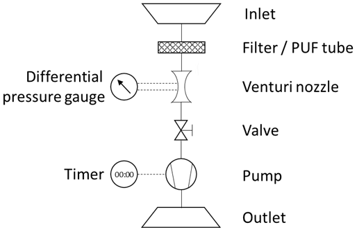
The following presents an educational approach explaining the general physical equations required to derive the concentration of airborne particulate-phase and gas-phase contaminants (e.g., pesticides, polychlorinated biphenyls, polychlorinated dibenzo-p-dioxins and furans, polycyclic aromatic hydrocarbons, flame retardants) with Hi-Vol air samplers. Figure 1 shows a typical device with its main components. An inlet is shielding the internals from the environment. Particles in the air are captured by a filter, which is permeable for the airflow but will retain particulate matter above a threshold size (depending on the filter type). Gas-phase contaminants are captured with tubes of polyurethane foam (PUF) or other adsorbent substrates (e.g., resin). A flow meter, such as a venturi nozzle with an attached differential pressure gauge, is required to determine the air flow velocity inside the device. The necessary vacuum to force air through the sampler is provided by a pump. A timer connected to the pump measures elapsed sampling time. The air flow rate can be adjusted with a valve. The air that has passed through these filters vents back to the atmosphere via an outlet exhaust pipe. The objective of this sampling is to determine a concentration C of a mass of contaminants m in a sampled volume of air V.
The mass of captured particles can be obtained by weighing the filter before and after the sampling. The weight difference Δm will be equal to the mass of captured particles. There is a large sensitivity of the concentration results to errors in weighing, hence special care is advised when handling the filters. When the mass of particles is known, they can be processed further to determine the mass of each contaminant by using various analytical techniques, e.g., those used for various flame retardants by Salamova et al. (2014). If contaminants in the gas phase are investigated, such as pesticides (Hermanson et al., 2007), additional analytical methods must be applied.
The second physical variable required is the volume of the sampled air V. This volume cannot be measured directly. Instead, it is derived by determining the volume of air passing through the sampler per unit time (volume flow rate ), multiplied with the sampling duration t.
The elapsed sampling time is quantified by using the timer clock mentioned above. The flow rate is determined using the continuity equation: assuming steady flow conditions, the flow rate can be calculated with the flow velocity v through a given flow cross section A.
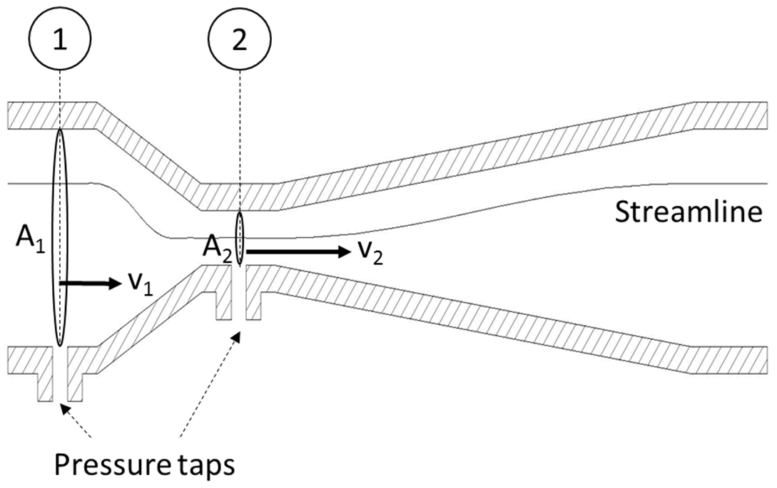
The flow velocity is measured with a flow device, such as a venturi nozzle or an orifice plate, shown in Figs. 2 and 3. These flow devices exhibit a specific geometry with a given inlet cross section 1 and a constriction 2 shown in Fig. 2. The areas of the cross sections A1 and A2 are known. By assuming continuity (no leaks), the flow rates through each cross section must be identical . Next, Bernoulli's principle of energy conservation is applied to derive the flow velocities from this system. Bernoulli is stating that for incompressible flow (such as in this example) the energy along a streamline is constant. The energy occurs in three different forms: as static pressure p, as dynamic pressure and as hydrostatic pressure ρgh, with the fluid density ρ, the standard gravity g and the hydrostatic height h.
Note that the hydrostatic pressure is omitted in this case because of the low density of air and a negligible hydrostatic height difference. The flow velocity v1 can be expressed by substituting v2 from the continuity equation into Bernoulli's equation. From this, the flow velocity is derived as a function of pressure difference between the two cross sections, density, and a constant dimensionless factor c1. The value of this factor can be quantified if the geometry of the flow device is known. However, as it will be shown below, it is not necessary to determine a numerical value. This is applicable for all constant factors that will be introduced throughout the following discussion.
To quantify the velocity v1 – which in turn will be used to calculate the volume flow rate and eventually the concentration C – two new variables must be determined. The differential pressure Δp can be measured easily with manometers, ranging from digital instruments to simpler devices such as U-tube manometers. The air density ρ cannot be observed directly and is derived using the ideal gas law, defined by ambient temperature T∞, ambient pressure p∞, and the specific gas constant for air R.
Ambient temperature is directly measured with a thermometer, and ambient pressure is measured with a barometer. Substituting density with the ideal gas law, Eqs. (3) and (6) can be summarized to the following.
Note that the constants, c2 and c3, are not dimensionless anymore. Equation (8) shows that the volume flow rate is dependent only on the ambient conditions and a pressure difference. Changes in temperature and pressure (i.e., air density) will affect the value of the sampled air volume. This is an unfavorable characteristic for Hi-Vol sampling because it implies that concentration results must be reported along with the ambient conditions during sampling. To allow for easier comparison between measurements, a standardized volume flow is introduced. The ambient-condition-specific volume flow rate can be converted to a standardized volume flow by applying the ideal gas law and the standard ambient conditions for temperature (T0=298.15 K) and pressure (p0=1013.25 hPa).
To underline that Eq. (9) is stating standardized volume flow, the pressure and temperature variables are presented as normalized, dimensionless terms, i.e., and . Finally, we can include all the above derivations into Eq. (1).

Equation (10) presents all variables required to be physically measured and necessary to derive the contaminant concentration: contaminant mass, sampling time, differential pressure at the flow device, ambient temperature, and ambient pressure.
The necessity of calibrating the volume flow rate arises from the fact that Eq. (10) contains the unknown constant c4. This constant not only represents the constant physical parameters but can also be used to account for second-order effects that have not been included in the equations, such as internal pressure loss, imperfect flow conditions, and flow obstructions. Assuming a direct proportional impact of these missing effects, a linear correlation can account for them and also the constant physical parameters. To define this linear correlation, a slope and an intercept must be found. This can be achieved by using a temporary calibration device to quantify the true, exact flow rate through the system at several pump pressures and to correlate that with Eq. (10). The linear correlation between the true flow rate with the unknown flow rate can be expressed by introducing a calibration slope (aCalibration) and calibration intercept (bCalibration) in Eq. (9).
The aim of the calibration process is to determine the numeric value of the calibration slope and intercept. First, the true flow through the air sampler is determined by using a temporary calibration device, typically with an orifice plate (Fig. 3). The true flow is evaluated at several flow rates (adjusted by regulating the pump voltage or the flow valve in Fig. 1). Second, the true flow rates are correlated to the differential pressure readings with the aforementioned linear approach in Eq. (11). The method is visualized in Fig. 4.
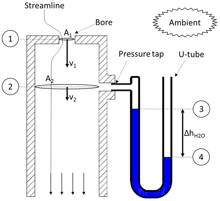
The calibration process will be described for the example of a Tisch Environmental Inc. TE-PUF polyurethane foam high-volume air sampler (Tisch, 2015). This sampling unit uses a venturi nozzle as a flow device and a Magnehelic® differential pressure gauge. For the calibration, an orifice calibrator is mounted on the sampler. The calibrator essentially consists of a cylindrical can with an orifice plate and a pressure tap (Fig. 3). Despite its simple construction, it is a highly accurate and robust calibration device (Wight, 1994).
To obtain the flow rate through the orifice calibrator , the same principles (continuity and Bernoulli between 1 and 2 in Fig. 3) are applied again. Following Eqs. (3)–(9), the orifice flow rate will depend on a pressure difference Δp between those two reference points. Instead of using a differential pressure gauge, this pressure difference is determined by using a U-tube manometer (slack tube). Bernoulli's principle (between 3 and 4 in Fig. 3) will be used to obtain this pressure difference from the U-tube manometer. One end of the manometer (3) is attached to the pressure tap on the calibration device (p3=p2), while the other end (4) is opened to ambient conditions ().
Note that the slack tube is filled with water (ρwater≈1000 kg m−3), hence the hydrostatic pressure term in the Bernoulli equation cannot be neglected anymore. Because the water in the U-tube is static (flow velocities are zero), the dynamic pressure term vanishes. Equation (14) for the orifice volume flow rate is very similar to Eq. (9). It contains an unknown constant of physical parameters: c5. To determine this constant, and to account for second-order effects, the same principle as for Eq. (11) is applied: the flow rate is correlated with a linear function.
The slope aOrifice and offset bOrifice are determined in a calibrated, laboratory environment, typically by the manufacturer of the orifice calibrator and provided as documentation for the orifice calibrator. Note that the orifice calibrator needs to be calibrated regularly by the manufacturer in order to maintain the calibration chain (laboratory–calibration device–sampler).
With the pressure difference from the U-tube manometer and the orifice slope and offset, can be calculated and the values correlated to the unknown device flow rate to obtain the true flow through the sampler , Eq. (11). For this, several observations n of the flow rate through the calibrator device and the sampler flow rate are taken. For each observation, readings of the differential pressure gauge (Magnehelic®) and the slack tube are taken.
The slope and intercept can be graphically determined by using a linear trend line and by plotting the results of the calibration measurements in a graph shown in Fig. 4. The x axis represents the flow rate for the orifice calibrator and the y axis the flow term for the internal flow device . The slope and the intercept of the resulting trend line are the sought-after calibration factors aCalibration and bCalibration in Eq. (11). As an alternative to the graphic solution, the following equations can be applied to numerically determine the slope and intercept.
The results are expected to show a very strong correlation because the flow through the orifice calibrator and the sampling device should be identical. A very low coefficient of correlation, e.g., r<0.990 (Tisch, 2015), could be an indication that there is an error in the system, such as a leak, which should be investigated before starting the measurements. The coefficient of correlation can be calculated with Pearson's equation or extracted from the graphical solution. Examples of the calibration calculations with numeric values can be found in various places in the literature, e.g., Tisch (2015) or APTI (1980).
There are several aspects that can lead to an erroneous calibration, related to operator mistakes and technical issues with the sampler. In both cases, the results obtained from the measurement may be meaningless. One way of identifying a flawed calibration is to operate two Hi-Vol samplers near each other (co-located sampling). This method is similar to analyzing duplicate laboratory samples and is expected to result in similar calibration results. When significant differences between the co-located samplers occur, the calibration procedure and the technical integrity of the samplers should be investigated.
This paper provides a missing piece of information in the literature regarding air sampling in the environment, showing that, by its nature, air sampling is a more complex process than sampling other environmental matrices. We have shown the variables and derivation of the equations used for calculating the air flow rate through a Hi-Vol air sampler and the process used for calibration of that flow rate. This allows investigators to identify the mass of contaminant found in a volume of air, once the analytical work has been completed. This detailed explanation of the process and equations allows a deeper understanding of the required variables and can be used for error estimation purposes.
No data sets were used in this article.
| The following symbols are used in this paper. |
| A=area [m2] |
| a=slope |
| b=intercept |
| c=constant |
| h=height[m] |
| m=mass[kg] |
| p=pressure [Pa] |
| t=time [s] |
| V=volume of air [m3] |
MH devised the idea for the paper, researched the literature, wrote the introduction, and provided feedback on the manuscript. RH developed the theoretical framework, derived the equations, wrote the paper, and prepared the figures.
The authors declare that they have no conflict of interest.
This work was originally prepared as part of the air sampling curriculum for the course “AT-331/831 Arctic Environmental Pollution – Atmospheric Distribution and Processes”, a Masters- and PhD-level course offered at the University Center in Svalbard (UNIS) from 2013 to 2017.
Financial support for Open Access was provided by the Norwegian University of Science and Technology (NTNU).
This paper was edited by Thomas F. Hanisco and reviewed by Kristie Ellickson and one anonymous referee.
Air Pollution Training Institute: APTI 435 Atmospheric Sampling, Student Manual, USEPA 450/2–80–004, 1980.
ASTM International: Standard test method for determination of gaseous and particulate polycyclic aromatic hydrocarbons in ambient air (collection on sorbent-backed filters with gas chromatographic/mass spectrometric analysis), D6209-13, 2013.
Basu, I., Arnold, K. A., Vernier, M., and Hites, R. A.: Partial pressures of PCB-11 in air from several Great Lakes sites, Environ. Sci. Technol., 43, 6488–6492, 2009.
Clements, H. A., McMullen, T. B., Thompson, R. J., and Akland, G. G.: Reproducibility of the HI-VOL sampling method under field conditions, J. Air Pollut. Control Assoc., 22, 955–958, 1972.
Danielson, J. A.: Air Pollution engineering manual, AP-40, US Department of Health, Education and Welfare, US Public Health Service, 1967.
Drinker, C. K., Warren, M. F., and Bennett, G. A.: The problem of possible systemic effects from certain chlorinated hydrocarbons, J. Indust. Hyg. Toxicol., 19, 283–311, 1937.
Hermanson, M. H. and Hites, R. A.: Long-term measurements of atmospheric polychlorinated biphenyls in the vicinity of Superfund dumps, Environ. Sci. Technol., 23, 1253–1258, 1989.
Hermanson, M. H., Monosmith, C. L., and Donnelly-Kelleher, M. T.: Seasonal and spatial trends of certain chlorobenzenes in the Michigan atmosphere, Atmos. Environ., 31, 567–573, 1997.
Hermanson, M. H., Scholten, C. A., and Compher, K.: Variable air temperature response of gas-phase polychlorinated biphenyls near a former manufacturing facility, Environ. Sci. Technol., 37, 4038–4042, 2003.
Hermanson, M. H., Moss D. J., Monosmith C. L., and Keeler G. J.: Spatial and temporal trends of gas and particle phase atmospheric DDT and metabolites in Michigan: Evidence of long-term persistence and atmospheric emission in a high-DDT-use fruit orchard, J. Geophys. Res.-Atmos., 112, D04301, https://doi.org/10.1029/2006JD007346, 2007.
Hites, R. A.: Atmospheric concentrations of PCB-11 near the Great Lakes have not decreased since 2004, Environ. Sci. Tech. Let., 5, 131–135, https://doi.org/10.1021/acs.estlett.8b00019, 2018.
Jutze, G. A. and Foster, K. E.: Recommended standard method for atmospheric sampling of fine particulate matter by filter media – high-volume sampler, J. Air Pollut. Control Assoc., 17, 17–25, 1967.
Lee Jr., R. E., Caldwell, J. S., and Morgan, G. B.: The evaluation of methods for measuring suspended particulates in air, Atmos. Environ., 6, 593–622, 1972.
Lynam, D. R., Pierce, J. O., and Cholak, J.: Calibration of the High-Volume Air Sampler, Am. Ind. Hyg. Assoc. J., 30, 83–88, 1969.
Monosmith, C. L. and Hermanson, M. H.: Spatial and temporal trends of atmospheric organochlorine vapors in the central and upper Great Lakes, Environ. Sci. Technol., 30, 3464–3472, 1996.
Salamova, A., Hermanson, M. H., and Hites, R. A.: Organophosphate and halogenated flame retardants in atmospheric particles from a European Arctic site, Environ. Sci. Technol., 48, 6133–6140, https://doi.org/10.1021/es500911d, 2014.
Salamova, A., Peverly, A. A., Venier, M. A., and Hites, R. A.: Spatial and temporal trends of particle phase organophosphate ester concentrations in the atmosphere of the Great Lakes, Environ. Sci. Technol., 50, 13249–13255, https://doi.org/10.1021/acs.est.6b04789, 2016.
Tisch Environmental: TE-1000 PUF Poly-Urethane Foam High Volume Air Sampler, Operations Manual, available at: https://tisch-env.com/wp-content/uploads/2015/07/TE-1000-PUF-Manual.pdf (last access: 29 August 2019), 2015.
US Environmental Protection Agency: Compendium of methods for the determination of toxic organic compounds in ambient air, 2nd edition, Compendium method TO-4A, EPA/625/R-96/010b, 1999.
US Environmental Protection Agency: Reference Method for the Determination of Suspended Particulate Matter in the Atmosphere (High-Volume Method), 40 CFR Appendix B to Part 50, available at: https://www.epa.gov/pcbs/method-4a-determination-pesticides, (last access: 30 August 2019), 2011.
Wight, G. D: Fundamentals of Air Sampling, CRC press, 1994.