the Creative Commons Attribution 4.0 License.
the Creative Commons Attribution 4.0 License.
 | 10 Sep 2019
peakTree: a framework for structure-preserving radar Doppler spectra analysis
Johannes Bühl
Patric Seifert
Hannes Griesche
Ronny Engelmann
Clouds are frequently composed of more than one particle population even at the smallest scales. Cloud radar observations frequently contain information on multiple particle species in the observation volume when there are distinct peaks in the Doppler spectrum. Multi-peaked situations are not taken into account by established algorithms, which only use moments of the Doppler spectrum. In this study, we propose a new algorithm that recursively represents the subpeaks as nodes in a binary tree. Using this tree data structure to represent the peaks of a Doppler spectrum, it is possible to drop all a priori assumptions on the number and arrangement of subpeaks. The approach is rigid, unambiguous and can provide a basis for advanced analysis methods. The applicability is briefly demonstrated in two case studies, in which the tree structure was used to investigate particle populations in Arctic multilayered mixed-phase clouds, which were observed during the research vessel Polarstern expedition PS106 and the Atmospheric Radiation Measurement Program BAECC campaign.


The characterization of mixed-phase clouds and associated microphysical processes poses a challenge to experimentalists, and therefore these processes are still not well represented in general circulation models (Fan et al., 2011). In situ instruments are subject to icing under the presence of supercooled liquid water, and the wide range of possible hydrometeor types requires the deployment of instruments that can each only cover a certain aspect of the whole hydrometeor distribution (Baumgardner et al., 2017; Korolev et al., 2017).
Cloud radars are frequently used for the investigation of mixed-phase clouds (Bühl et al., 2017). At Ka and W band, cloud radars are sensitive to scattering from the whole range of possible hydrometeors, ranging from cloud droplets to graupel (e.g., Kollias et al., 2007a; Fukao and Hamazu, 2014). In general, cloud radars are Doppler-capable and provide the backscattered signal as a function of Doppler velocity, commonly called the Doppler spectrum (Wakasugi et al., 1986). When multiple particle populations are present in the observed volume, they are frequently represented as distinct peaks in the Doppler spectrum (e.g., Shupe et al., 2004; Luke et al., 2010; Verlinde et al., 2013; Yu et al., 2014; Kalesse et al., 2016; Kollias et al., 2016). The properties of a multi-peak situation can only partly be represented by the moments of a single-peak algorithm, which causes errors in the target classification and subsequent microphysical retrievals. A multitude of approaches are available to classify clouds and retrieve water contents, particle sizes and number concentrations (for example, Clothiaux et al., 2000; Wang and Sassen, 2002; Wang et al., 2004; Hogan et al., 2006; Illingworth et al., 2007; an overview is provided in Shupe et al., 2016, and Zhao et al., 2012). Almost all established algorithms are based on the assumption of mono-modal hydrometeor size distributions, which likely causes significant errors in multi-peaked situations.
The analysis of multi-peaked Doppler spectra can be separated into three steps.
-
Peak identification (or peak finding). Locate the boundaries of a (sub)peak.
-
Peak structuring. Identify the arrangement of the (sub)peaks.
-
Peak interpretation. Categorize and interpret the peaks.
Most available methods focus either on the peak identification or the peak interpretation step. For peak identification either noise-floor-separated peaks and/or local minima in the spectral reflectivity are used (Shupe et al., 2004; Rambukkange et al., 2011). More sophisticated approaches allow for a separation of multimodal peaks. This is done, for example, by using skewness signatures (Luke and Kollias, 2013) or continuous wavelet transforms (Luke et al., 2010; Yu et al., 2014). Recently, Kalesse et al. (2019) proposed an algorithm for subjective peak identification criteria using machine learning.
Structure is reflected by a linear list of all subpeaks, usually sorted by velocity or reflectivity. In a further step, Oue et al. (2018), using the microARSCL algorithm (Kollias et al., 2007b; Luke et al., 2008), allow a primary peak to be split into two subpeaks. But they constrain the structure by assuming the left peak (faster falling peak) to have a higher reflectivity. Additionally, a noise-floor-separated secondary peak is possible, but this one is assumed to be mono-modal. Such strong constraints may be justified for short periods at single geographic locations but are not suitable for a general approach. Currently, no generic and flexible formalism is available to describe an arbitrary number of subpeaks of a Doppler spectrum without a priori assumptions on the structure.
In the peak interpretation step, the peaks are usually sorted into categories using their moments. Categories are, for example, one liquid and one ice peak (Shupe et al., 2004), liquid, newly formed ice, ice from above (Rambukkange et al., 2011), or liquid and two ice populations (Oue et al., 2018).
This study will focus on the second step, peak structuring. It will be shown that a binary tree representation of multiple peaks can provide a rigid and hence flexible formalism for structuring the peaks in a Doppler spectrum. The tree structure allows for an arbitrary number of subpeaks in any arrangement, while at the same time being unambiguous and easily accessible by algorithms. The software implementing the algorithm is easily applicable to other radar systems and available openly. The study is structured as follows: the datasets used for demonstration are introduced in Sect. 2. In Sect. 3, the binary tree peak-structuring algorithm is presented. Section 4 is dedicated to the presentation of two case studies in which the algorithm was used to investigate Arctic mixed-phase clouds. Discussions and conclusions are covered in Sect. 5.
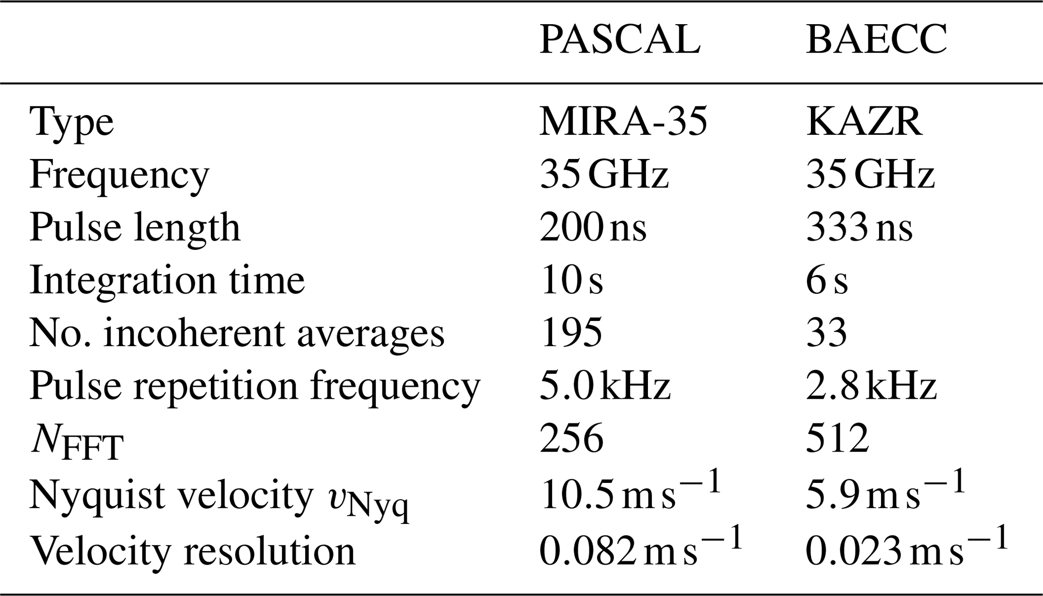
The binary tree peak-structuring algorithm is applied to two datasets using Ka band radars from different manufacturers with slightly different settings. Details on the instruments and datasets are given here.
2.1 MIRA-35 during PASCAL
During the Physical feedbacks of Arctic planetary boundary level Sea ice, Cloud and AerosoL (PASCAL) campaign (PS106; Wendisch et al., 2019) a cloud radar of the MIRA-35 type was operated as part of the OCEANET suite on R/V Polarstern together with, amongst other instruments, a PollyXT Raman and polarization lidar (Engelmann et al., 2016) and a HATPRO 14-channel microwave radiometer (Rose et al., 2005). MIRA-35 is a magnetron-based pulsed 35 GHz cloud radar with polarization and Doppler capabilities (Görsdorf et al., 2015). During the campaign, MIRA-35 was operated in linear depolarization ratio (LDR) mode. The pulse repetition frequency was 5 kHz and one raw Doppler spectrum was based on the fast Fourier transform of 256 pulses, yielding a Doppler resolution of 0.082 m s−1 (Table 1). The radar was operated in vertical-pointing mode. It was based on a leveling platform that actively corrected for the pitch and roll movement of the ship. Vertical movement of the radar was corrected at a rate of 4 Hz using the ship motion data originally recorded at 20 Hz. For the datasets of Arctic clouds presented here, active stabilization was no longer available due to a hardware failure. In the scope of this study, the Doppler spectra acquired within 10 s were therefore averaged incoherently to suppress the ship pitch and roll motion, while the vertical motion was still corrected at a rate of 4 Hz. The lack of active pitch and roll suppression led to an accuracy of the zenith pointing of 1.5∘. For horizontal wind velocities below 10 m s−1, the bias introduced to the observed vertical velocity is thus below 0.2 m s−1.
By default, MIRA-35 provides noise-cleaned compressed Doppler spectra (zspc) and moment data separately for meteorological targets and atmospheric plankton (Görsdorf et al., 2015). Further data analysis is subject to the operator of the cloud radar, to which the zspc data provides a solid base for potential application of peak separation techniques. Accurate measurements of polarization variables, like the LDR, depend strongly on instrument hardware due to polarization leakage. The lowest LDR observable (integrated cross-polarization ratio – ICPR) with this version of MIRA-35 was estimated in the presence of light drizzle with the approach of Myagkov et al. (2015) and found to be −27.6 dB. A second effect that has to be considered while calculating the LDR is the noise level in the cross-polarized channel. If the signal in the cross-polarized channel is below the noise level, the LDR is determined solely by the signal in the co-polarized channel and no meaningful information on the polarization state of the received signal can be derived (Matrosov and Kropfli, 1993). Hence, when calculating the LDR (Eq. A6) only bins in which the signal in the cross-polarized channel is a factor of 3 above the noise level are taken into account.
2.2 KAZR during BAECC
The Biogenic Aerosols–Effects on Clouds and Climate (BAECC) campaign (Petäjä et al., 2016) was a deployment of the U.S. Department of Energy’s Atmospheric Radiation Measurement (ARM) Mobile Facility (AMF) to Hyytiälä (61.9∘ N, 24.3∘ E), Finland, from February to September 2014. A vertical-looking Ka-band ARM zenith radar (KAZR) 35 GHz cloud radar (Kollias et al., 2016) was part of the remote sensing instrumentation of the AMF. It was operated at a pulse repetition frequency of 2.8 kHz. The Doppler resolution is 0.023 m s−1, as a 512-point fast Fourier transform was used to estimate the Doppler spectra (Table 1). The vertically pointing KAZR used in this campaign does not possess a cross-polarized channel, and hence no polarimetric variables are available.
Table 1Configuration settings of the two cloud radars used in this study.
3.1 Transforming the Doppler spectrum into the tree structure
The algorithm explained here transforms each Doppler spectrum with its (sub)peaks into a full binary tree structure. A full binary tree is a directed graph with one root node, and recursively each node might possess either two child nodes or none (Garnier and Taylor, 2009). Each node can be identified by an index, which is based on level-order tree traversal. The index i of a node can be calculated by the following formulas:
with the floor function ⌊ ⌋. These indices are illustrated in Fig. 1. This example shows a complete binary tree, meaning all nodes are present. When applied, some indices, e.g., 9 and 10 or 5, 6, 11, 12, 13 and 14, might be missing. However, the rule “a node might possess either two child nodes or none” always holds.
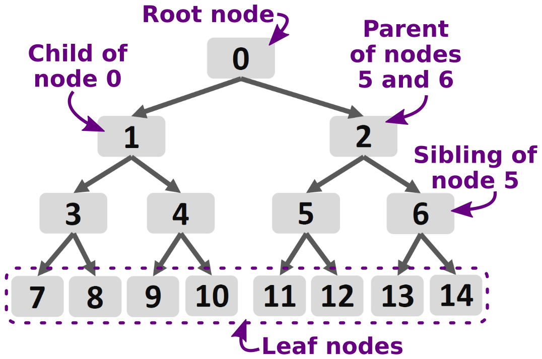
Figure 1Binary tree containing 15 nodes with possible indices according to level-order tree traversal.
Applied to radar Doppler spectra, a node is related to a part of the Doppler spectrum that contains at least one peak. The peak boundaries are identified (step 1 as listed in Sect. 1) by a noise-floor threshold and local minima in the spectral reflectivity (or spectral power density). These boundaries are then used to construct the tree structure (step 2 as listed Sect. 1). The root node contains all signal of the Doppler spectrum above the noise threshold. Two example spectra from KAZR and MIRA-35 are shown in Fig. 2a and b, respectively. The boundaries and moments for the MIRA-35 and KAZR are listed in Tables 2 and 3, respectively. In a first step, all noise-floor-separated peaks are added as child nodes with their boundaries vleft and vright (in the example for MIRA-35 −3.30 and 1.32 m s−1). Each node is then checked for (sub)peaks within using the peak boundaries from the lowest to the highest spectral reflectivity. Starting with the lowest minimum at vadd, the node containing this minimum is split into two child nodes. When boundaries of the parent node are [vleft,vright], the left child node is [vleft,vadd] and the right child node is [vadd,vright]. In the example from Fig. 2b the internal minimum with the lowest spectral reflectivity is at with a spectral reflectivity of −33.4 dBZ. This reflectivity also defines the threshold that separates the subpeaks. The splitting at local minima is repeated for all remaining minima, always splitting the leaf node (i.e., a node that does not have any child nodes) in which the minimum is located.
A minimum is skipped if the prominence of either of its subpeaks is less than 1 dB. Prominence is the difference between the maximum spectral reflectivity of a subpeak and the threshold that is defined by the spectral reflectivity at local minimum (dashed grey lines in Fig. 2a, b; similar to Shupe et al., 2004).
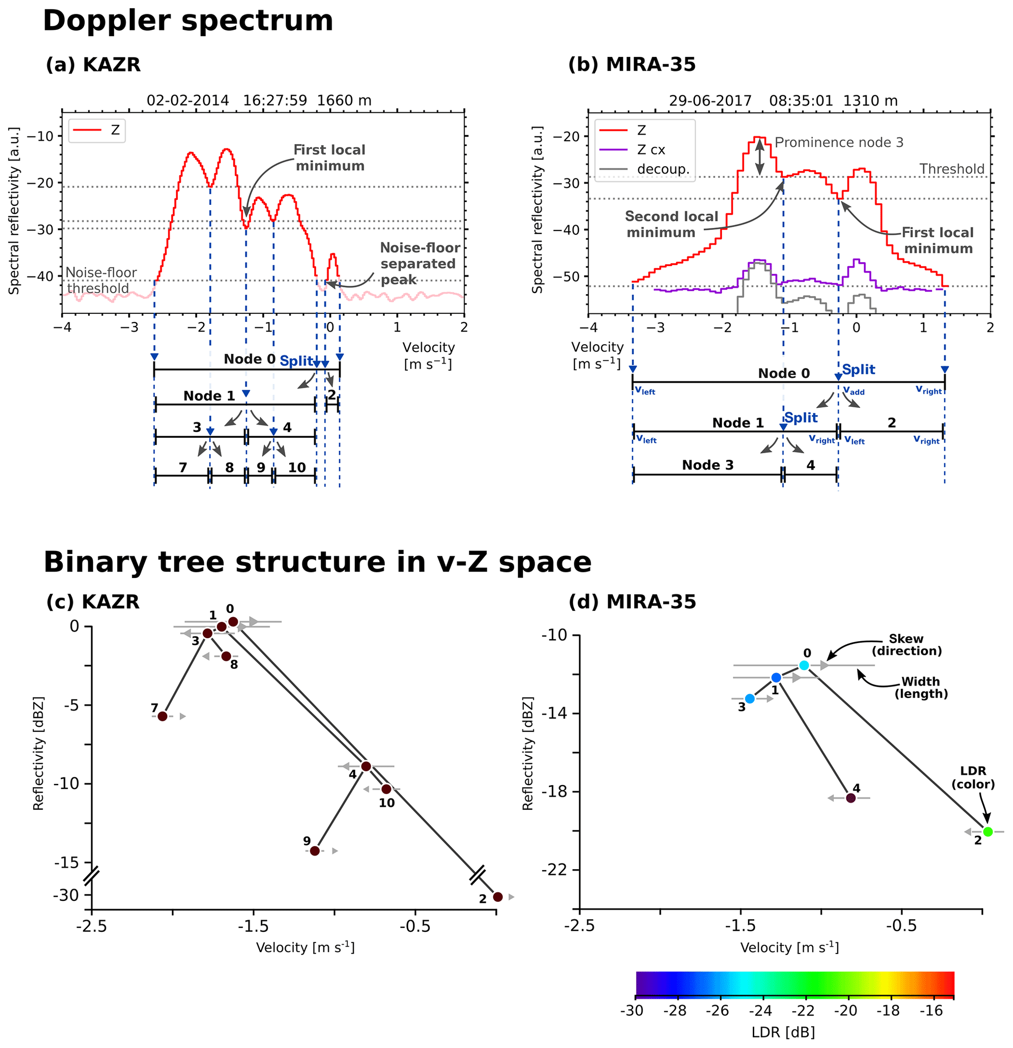
Figure 2Example for generating the trees for two Doppler spectra from different cloud radars of type KAZR (a, c) and MIRA-35 (b, d). The root node (node 0) is split into child nodes at the indicated velocity bins (dashed blue), which contain a local minimum in spectral reflectivity. The threshold defined by the noise floor and the internal minima is marked with dashed grey lines. In the spectrum in (b) the reflectivity in the cross-polarized channel (Z cx) is shown together with the co-polarized channel signal subtracted by the polarization decoupling (further explanation in Sect. 2.1). Panels (c) and (d) show the resulting trees, for which the location of a node in the v−Z space is based on its moments. Spectral width is indicated quantitatively by the length of the grey lines, and the sign of the skewness is indicated by a triangle (pointing left for negative skewness and vice versa). The circle denoting the node position is color-coded in accordance with the node LDR.
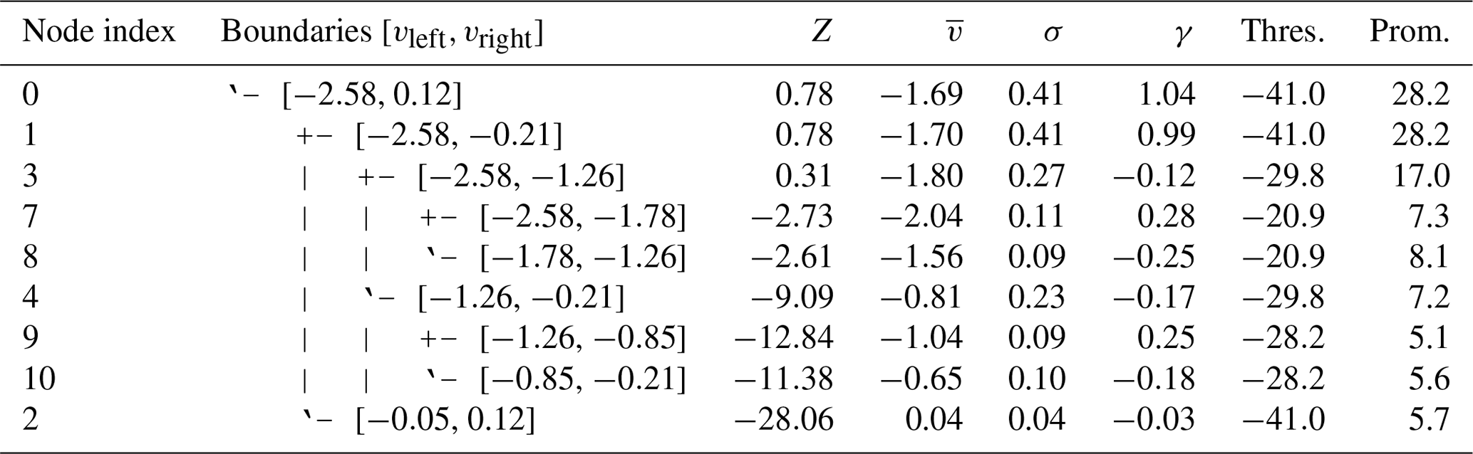
Table 2Moments for each peak from the MIRA-35 Doppler spectrum depicted in Fig. 2b with the index of the node according to the level-order tree traversal and the boundaries vleft and vright in m s−1. Child nodes are denoted by their level of indentation. The units are dBZ for reflectivity Z and m s−1 for and spectral width σ. The skewness γ is dimensionless; LDR is in dB. The threshold “Thres.” is in dBZ and the prominence “Prom.” is in dB.
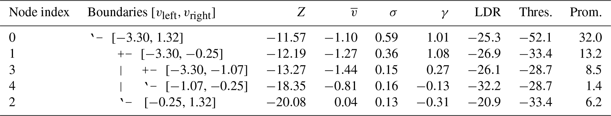
Table 3Moments for each peak from the KAZR Doppler spectrum depicted in Fig. 2a; similar to Table 2.
In the next step, the moments of the Doppler spectrum (reflectivity, mean velocity, width, skewness) are calculated for each node within its boundaries [vleft,vright] (see Appendix A). The equivalent reflectivity factor Z (the subscript e is omitted for brevity) is calculated by integrating the spectral reflectivity of the whole peak (i.e., from the noise floor up). For all higher moments, the signal below the threshold that separated the (sub)peak is neglected to avoid biases (see also Fig. A1). The LDR for each node is calculated using the spectral reflectivity in the cross-polarized channel if such a channel is available.
Node 0 contains all components of the Doppler spectrum that are above the noise threshold. In general, this node is similar to the moment estimation commonly used to analyze Doppler spectra (e.g., Carter et al., 1995; Clothiaux et al., 2000; Görsdorf et al., 2015). Only in the case of the presence of noise-separated subpeaks within node 0 do some moment estimators such as microARSCL apply the moment retrieval to the most significant peak only. The child nodes (1 and 2) of node 0 are the subpeaks defined by the lowest relative minimum. The second lowest minimum then splits one of these nodes and gives nodes 3 and 4 (splitting node 1) or 5 and 6 (splitting node 2). The total number of subpeaks nsubpeaks, as estimated by established peak-finding methods, can be calculated from the number of nodes nnodes:
Each node is characterized by its reflectivity Z, vertical velocity v, spectral width, skewness, LDR and prominence. It is suitable to visualize the tree in the v−Z plane as a color-filled circle with the parent–child relationships depicted by a black line (Fig. 2c and d) and each circle is color-coded in accordance to its LDR (if available as for MIRA-35). The width and skewness are shown by a horizontal grey line and a grey triangle with varying size, respectively. This representation hence combines all key parameters of a multi-peak Doppler spectrum.
3.2 Peak interpretation
Once the tree structure is constructed, various methods for peak interpretation can be used. In this study only two rather basic approaches are shown.
3.2.1 Selecting cloud droplet nodes
Nodes that are most likely caused by liquid droplets can be identified by their moments, as already done in previous studies (e.g., Frisch et al., 1995; Shupe et al., 2001; Rambukkange et al., 2011; Yu et al., 2014; Kalesse et al., 2016). The liquid cloud droplets are assumed to be small and only possess a negligible terminal velocity. In the absence of strong vertical air motions the (sub)peak caused by the liquid droplets will be close to 0 m s−1. Additionally, due to their small size, the reflectivity of these droplets is rather small. Combining these characteristics, a simple selection rule is based on two thresholds: and . Using these criteria, each node in a tree can be checked and the index of the fitting node is stored. This selection process can be used on larger time–height slices in a straightforward and computationally efficient way, identifying regions of a cloud where liquid droplets cause a distinguishable (sub)peak.
3.2.2 Grouping nodes into particle populations
The nodes representing similar particle populations in neighboring (time–height) bins can be connected to obtain a continuous picture of the evolution of a particle population. First, a node is manually assigned to a particle population based on visual inspection and guided by the LDR value. These manually selected (anchor) nodes are spaced in steps of 50 s and 150 m, making one anchor representative for a slice of five time steps and five height bins or, in other words, for the 25 neighboring trees. For the time–height bins between these anchor nodes, nodes with similar characteristics of the moments are automatically selected. A node is considered similar to the anchor node if the Euclidean distance d in the v−Z space is minimal and below a threshold d<0.9. For the present study, the parameters Z and v are normalized by factors of 5 and 0.3, respectively, to make both comparable for the grouping algorithm (Fig. 3). The sibling of each selected node is afterwards assigned to the complementary particle population.

Figure 3Illustration of the grouping algorithm for one anchor node. Single trees for a time–height slice of MIRA-35 observations are depicted in (a) with the selected anchor node marked by an arrow. The time–height cross section shown omits the outer trees of the 5×5 slice for clarity. The moments of each node are illustrated, as described in Fig. 2. In (b), the trees are combined into the same v−Z illustration with a circle denoting the nodes that are identified as similar by the Euclidean distance criterion. The Euclidean distance d is depicted in inset (c) for all nodes with index 2.
4.1 KAZR case, 2 February 2014: identifying embedded liquid layers
On 2 February 2014 an intense low-pressure system over the Faroe Islands together with a high-pressure core above southwestern Russia caused southerly flow over Finland. Low-level clouds were observed the whole day. During the afternoon an occluded front with a cold frontal character reached the Hyytiälä field site (further description also in Kalesse et al., 2019). Frontal precipitation started at 14:30 UTC and was caused by two geometrically deep cloud systems, both topped around a height of 8 km with a short pause in between. The first precipitation event was characterized by liquid precipitation with a melting layer around a height of 1.2 km (not shown), but for the second event from around 15:30 UTC onwards snow precipitation dominated. Fig. 4 shows a part of the frontal system. Between 16:00 and 16:20 UTC a lower cloud with an almost constant cloud top at a height of 2.6 km was observed. In this cloud, reflectivity and vertical velocity are increasing toward the ground. At 16:18 UTC ice crystals from the top cloud start to sediment into this lower cloud. At a height of 2.2 km, the vertical velocity of these particles increases up to (Fig. 4b). The total number of nodes (Fig. 4c) reveals that the cloud radar Doppler spectra were dominated by multi-peaked situations, predominantly in the lower layer. Up to nine nodes were found, which corresponds to five subpeaks.
The selection rule described in Sect. 3.2.1 is now used to identify nodes that are likely caused by liquid droplets. Figure 5 shows the moments of the liquid droplet nodes. Two liquid layers become visible, a lower one between a height of 0.8 and 1.3 km and a higher one with more irregular boundaries between a height of 1.6 and 2.6 km. The vertical velocity (Fig. 5) shows the typical pattern of small particles with negligible terminal fall velocity, which follow the air motion. Areas of updrafts and downdrafts with velocities between −0.5 and are clearly visible.
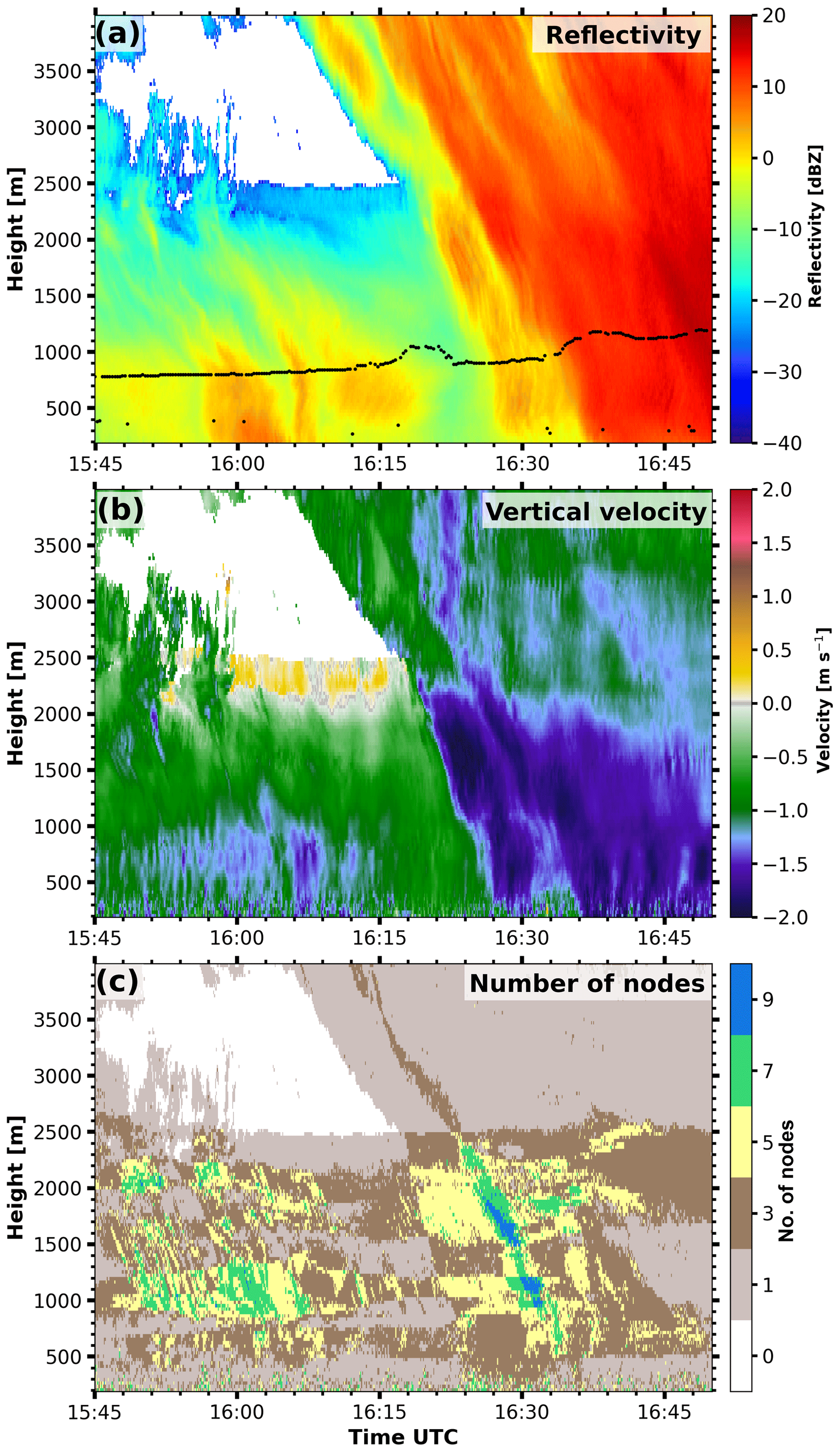
Figure 4KAZR reflectivity with lidar-detected cloud-base height (black dots, a), mean velocity (b) and number of nodes (c) on 2 February 2014 from 15:45 to 16:45 UTC.
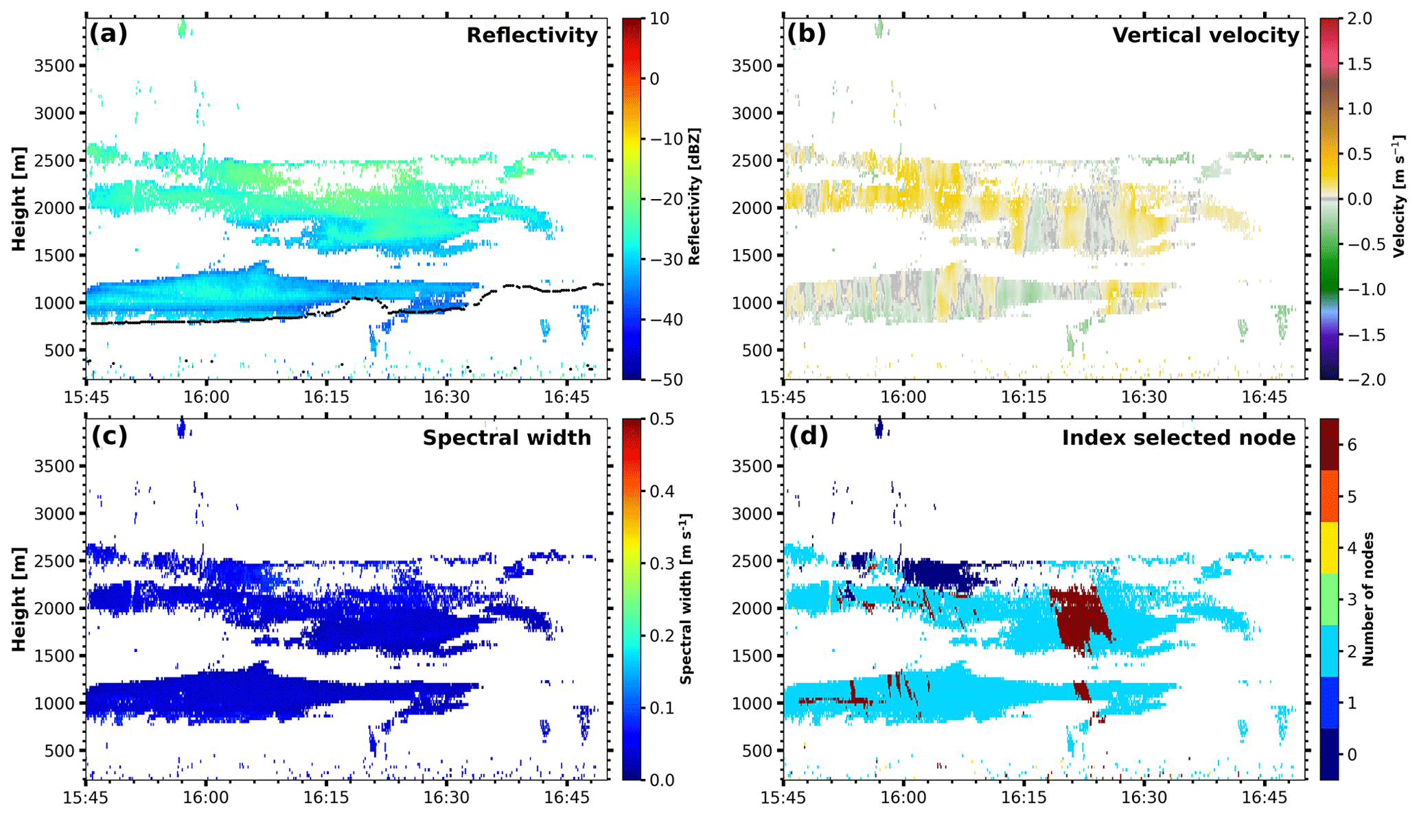
Figure 5KAZR reflectivity with lidar-detected cloud-base height (black dots, a), mean velocity (b), spectral width (c) and index of node (d) for nodes identified as liquid cloud drops on 2 February 2014 from 15:45 to 16:45 UTC.
4.2 MIRA-35 case, 29 June 2017: separating two ice crystal populations in an Arctic cloud
On 29 June 2017 R/V Polarstern was located a few nautical miles north of the island of Kvitøya at 80.5∘ N, 31.5∘ E and operated in the framework of the PASCAL campaign. The synoptic situation was controlled by a low over Fram Strait with a secondary low that passed Polarstern on that day, with the surface wind veering from SE to NW and frequent light precipitation.
Between 08:30 and 09:45 UTC a cloud was continuously observed by MIRA-35 from the surface up to a height of 2.7 km with a cloud-top temperature of −15 ∘C (see Fig. 6). The thermodynamic structure of the cloud was probed by a RS92-SGP radiosonde that was launched from Polarstern at 10:50 UTC (Schmithüsen, 2017). The spread between temperature and dew point (Fig. 6a) shows saturation with respect to liquid water throughout the whole cloud. Very light precipitation was observed at the surface by an optical disdrometer (Klepp et al., 2018), peaking at 0.1 mm h−1 at 08:50 UTC. The highest values of liquid water path (), obtained from the microwave radiometer (Rose et al., 2005), were also observed during this time. Low reflectivity and vertical velocities close to 0 m s−1 with alternating updrafts and downdrafts suggest the presence of a turbulent liquid layer capping the cloud. Below a height of 1.3 km, the reflectivity and LDR of the single-peak analysis show a sharp increase, giving hints regarding a change in microphysical properties, such as size or shape.

Figure 6Radiosonde ascend on 29 June 2017 at 10:50 UTC (a, d from Schmithüsen, 2017). MIRA-35 reflectivity with lidar-detected cloud-base height (black dots, b), mean velocity (c) and linear depolarization ratio (e) of the zeroth node (moments of the single-peak analysis) on 29 June 2017 from 08:30 to 09:45 UTC. Total number of nodes (f) for the same period.
Application of the multi-peak analysis introduced above reveals that multi-peak spectra were quite frequent (Fig. 6f). Figure 7 shows the nodes identified as caused by liquid droplets according to the selection rule from Sect. 3.2.1. Two continuous liquid layers at almost constant heights were observed during the whole event. The uppermost layer at a height of 2.7 km topping the cloud is also visible in the moments of the full spectrum. The lower layer at a height of 1.3 km is hidden when only using the moments of the full spectrum. Furthermore, shorter periods with likely liquid water presence were detected, for example from 08:55 to 09:15 UTC at a height of 1.0 km. Additionally, the ceilometer-detected cloud base (Fig. 7a, black dots) indicates the base of the liquid layer at a height of 750 m between 08:40 and 09:15 UTC. This lower part of the liquid layer did not produce a distinguishable (sub)peak in the Doppler spectrum and therefore no individual node.

Figure 7MIRA-35 reflectivity with lidar-detected cloud-base height (black dots, a), mean velocity (b) and index of node (c) for nodes identified as liquid cloud drops by the selection rule from Sect. 3.2.1 on 29 June 2017 from 08:30 to 09:45 UTC.
After grouping the nodes to particle populations (as explained in Sect. 3.2.2), the microphysical structure of this cloud becomes clearer. The faster-falling particle population (Fig. 8, left column) originating at the uppermost liquid layer at a height of 2.7 km has a rather variable reflectivity with background values of around −20 dBZ and maxima in frequently occurring fallstreaks of up to 0 dBZ reflectivity. The vertical velocity (Fig. 8c) is quite variable as well. Below a height of 2.5 km, the ice particles generated at cloud top descend with velocities of −0.5 and . The low LDR of these particles (Fig. 8e) is characteristic for oblate or plate-like particles (Myagkov et al., 2016), which is also consistent with particle shapes formed at cloud-top temperatures of around −15 ∘C (Bühl et al., 2016). Below the height of primary ice formation, several processes, like depositional growth and aggregation, might contribute to particle growth.
Frequently, fallstreaks from the upper layer penetrate the second liquid layer at a height of 1.3 km. The lower-level liquid layer with a temperature of −5 ∘C also continuously forms ice (Fig. 8, right column). The vertical velocity (Fig. 8d) is lower () and more homogeneous than for the other particle population. The high LDR of −14 dB at heights of 100 to 200 m below the top of the liquid layer can be attributed to prolate or columnar ice crystals (Myagkov et al., 2016; Bühl et al., 2016). Hence, ice formation takes place between a height of 1.1 and 1.3 km, which is also underpinned by the gradual increase in reflectivity and vertical velocity toward the ground. Below a height of 1.1 km, the reflectivity is more variable, with maxima of 9 dBZ at 08:50 UTC and minima of −11 dBZ at around 09:10 UTC. We cannot fully rule out from the information given the possibility that ice multiplication was triggered when the higher-level ice particles descended into the lower liquid layer. However, ice was formed from the lower liquid layer constantly over time (Fig. 8, right column), even in periods during which particles with very low reflectivity were potentially seeding from above, as was the case, for example, between 09:10 and 09:30 UTC. This supports the interpretation that at least a few ice crystals were caused by primary ice formation.
Looking into two individual fallstreaks, it is possible to track the evolution of the two particle populations. The selected fallstreaks are illustrated as black dashed curves in Fig. 8. In the framework of this study, the fallstreaks were tracked manually based on the criterion of following the maximum of the radar reflectivity of the faster-falling (and also oblate) particle population. It should be noted that techniques for an automated classification of fallstreaks exist (Kalesse et al., 2016; Pfitzenmaier et al., 2017), which should be applied when longer time series are analyzed. But these algorithms have shortcomings when strong directional wind shear is present, as in this case (Fig. 6d). The first hints for different microphysical processes become evident from tracking the properties of the individual nodes in the selected fallstreaks. The first one starts at 08:52 UTC and a height of 1.8 km with oblate particles having a rather constant reflectivity of −5 dBZ and a vertical velocity of around . The reflectivity of this population is almost constant down to a height of 0.9 km, even after the fallstreak reaches the lower liquid layer. The LDR is unaffected by the liquid layer as well. Contrarily, the prolate particle population generated within this liquid layer shows a strong increase in reflectivity from −20 to +6 dBZ, while LDR decreases from −14 to −19 dB. Below a height of 0.8 km, the faster-falling mode (low LDR) is no longer visible as a separate peak (and accordingly the node disappears) because the slower-falling population (one with high LDR) becomes dominant in the Doppler spectrum.
The second fallstreak, being less pronounced than the first one, begins at 09:06 UTC and a height of 1.5 km with a reflectivity of −10 dBZ and again a vertical velocity of around for the oblate particles. After reaching the liquid layer at a height of 1.3 km, the reflectivity of this particle population increases to −7 dBZ and the velocity also increases slightly. The LDR remains below −25 dB. The second particle population with a prolate shape grows as well from less than −20 dBZ in the liquid layer to −4 dBZ at 0.6 km with a final velocity of . During this growth, LDR remains at the high value of −14 dB, indicating no change in the particle shape. Due to insufficient polarimetric data, especially the lack of scans, it is difficult to disentangle the contribution of different microphysical processes to particle growth. A more detailed investigation, using synergistic retrievals on top of the algorithm presented here, is required to pin down the relevant processes further.
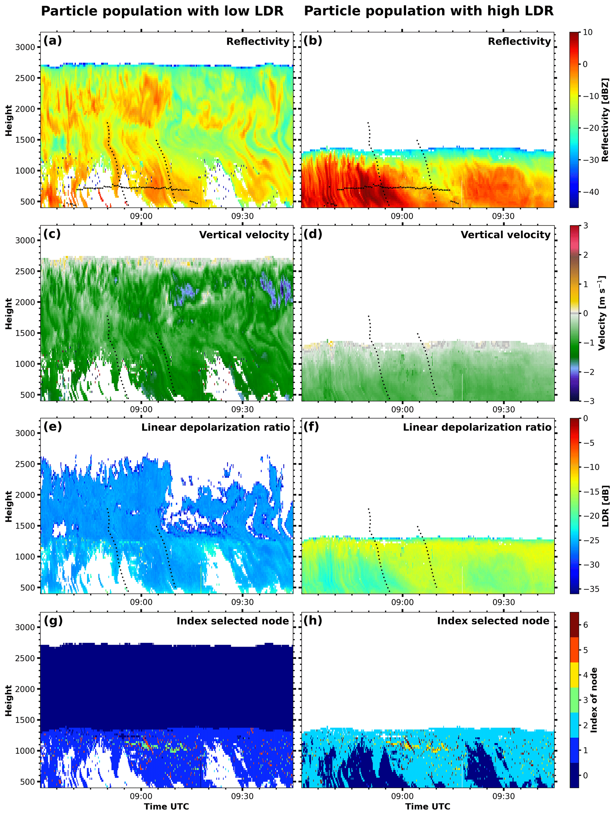
Figure 8MIRA-35 reflectivity with lidar-detected cloud-base height (black dots, a, b), mean velocity (c, d), linear depolarization ratio (LDR; e, f) and index of the selected node (g, h) of the two particle populations (left and right column) on 29 June 2017 from 08:30 to 09:45 UTC. The dashed black lines locate the two fallstreaks described in the text. For regions marked in white no node could be assigned to the respective particle population.
The ice water content (IWC) for each particle population can be retrieved from Z and the temperature (Hogan et al., 2006). This Z−T retrieval was developed under the assumption of mono-modal peaks in the Doppler spectrum, but using the tree structure it is possible to include the information from the Doppler spectrum into this retrieval rather easily. Figure 9 shows the IWC for node 0 or the full Doppler spectrum (a), hence assuming single-peaked spectra. Applying the IWC retrieval for the separated particle populations reveals the relative contribution of one population to total ice mass (Fig. 9b). As can also be seen in the discussion on the reflectivity of the particle populations above, the precipitation reaching the ground between 08:30 and 09:00 UTC could not be directly linked to cloud top (2.7 km), as the whole ice mass below a height of 1.3 km can be assigned to the prolate particle population. Contrarily, between 09:00 and 09:15 ice mass was almost equally distributed to both particle populations below a height of 1.3 km. Following this approach, the proposed technique can also be used to extend the capabilities of other established retrieval algorithms.
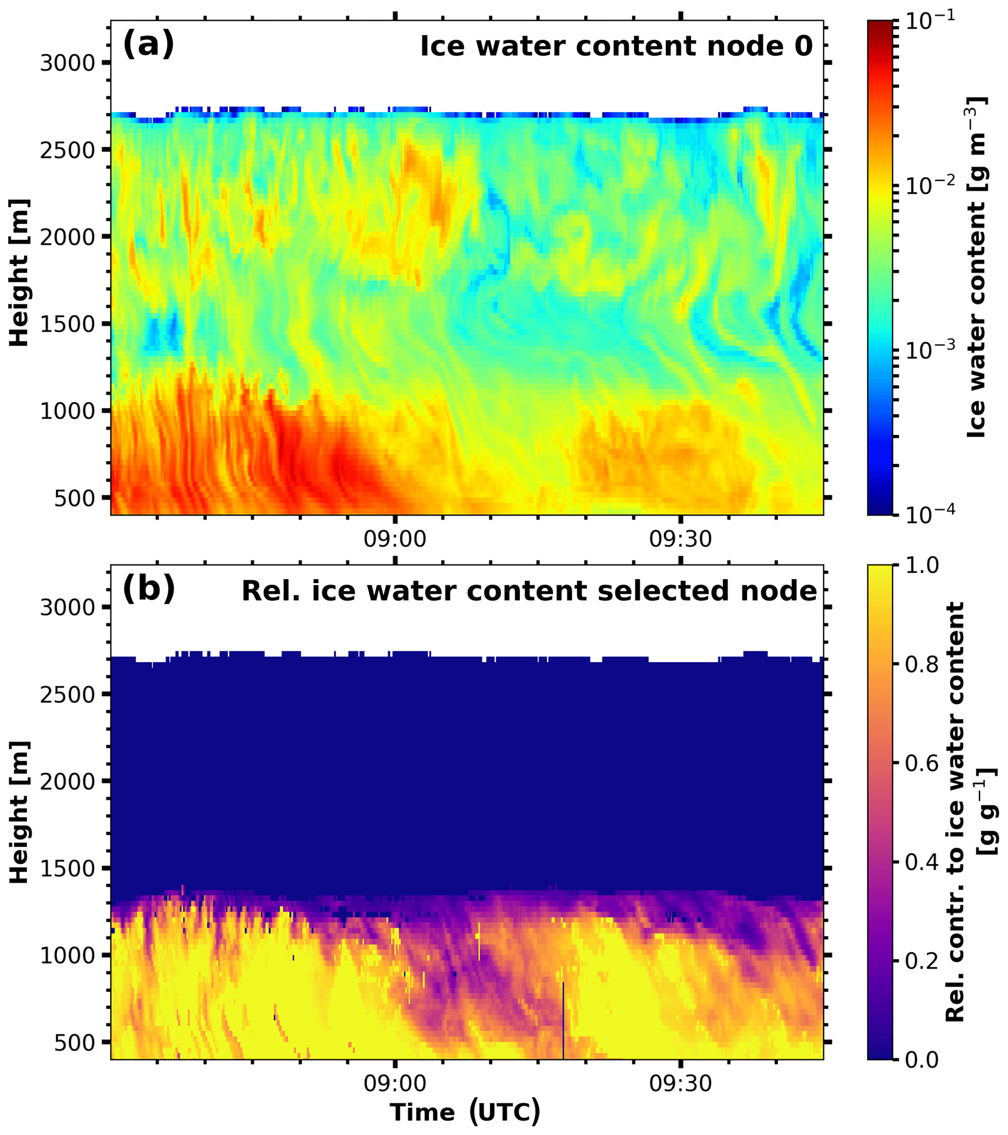
Figure 9Retrieved ice water content from node 0 (a) and the relative contribution of the particle population with high LDR (b) on 29 June 2017 from 08:30 to 09:45 UTC.
We proposed a binary tree structure for individual peaks of a multi-peaked cloud radar Doppler spectrum. This data structure does not require prior assumptions on the arrangement or hierarchy of the peaks. The tree structure allows for the selection of the level of complexity with which the Doppler spectrum is approximated by the number of nodes taken into account. It also provides backward compatibility, as the root node (i.e., node 0) holds the moments of the full Doppler spectrum with an implicit assumption of mono-modality. These moments are similar to standard Doppler spectra processing. Hence, a seamless transition from current single-peak techniques to multi-peak analysis is possible. The recursive structure of the tree allows the artificial separation into noise-floor-separated peaks and subpeaks within noise-floor-separated peaks to be dropped, as was necessary in prior approaches (see Fig. 13 in Williams et al., 2018). This separation imposed strong constraints on structure without having a physical reason. For example, depending on the intensity of turbulence, two noise-floor-separated peaks might appear only as (sub)peaks of one peak in the Doppler spectrum.
We showed two basic techniques to demonstrate how the tree structure can be utilized for peak interpretation (step 3 as defined in Sect. 1). The first technique used a simple selection rule to identify peaks that are most likely caused by liquid water. The choice of the threshold is based on prior studies. For reflectivity, the −20 dBZ threshold as used by Oue et al. (2018) and reported by Kalesse et al. (2016) is rather conservative compared to older studies (e.g., Frisch et al., 1995; Kogan et al., 2005; Yu et al., 2014). The velocity threshold depends strongly on the dynamical environment. The threshold of might only be valid for stratiform conditions, as in the two case studies shown. Good agreement with the ceilometer-derived cloud-base heights in the KAZR case (Sect. 4.1) is in agreement for other studies using a comparable threshold. Similar rules can potentially be applied for other particle types with a clear signature in the moments of the Doppler spectrum, as might, for example, be the case for heavily rimed particles.
The second technique grouped nodes from neighboring Doppler spectra into particle populations based on their moments using the Euclidean distance in v−Z space. The thresholds used here depend strongly on the conditions they are applied to. The normalization factors for reflectivity Z and velocity v weight the variation in one dimension with respect to the other. For this case, changes in velocity were only allowed to be relatively small compared to changes in reflectivity. Considering only changes along one axis, reflectivity could vary by 4.5 dBZ for neighboring trees for two nodes and still be considered to belong to the same particle population, whereas velocity could only vary by 0.27 m s−1. The distance threshold d controls gaps in the grouping. A low distance threshold would select only a subset of nodes, introducing gaps in time and range for the grouped particle population. A high distance threshold can make the selection ambiguous, as two or more nodes in one tree might fulfill this condition. The frequency of anchor nodes is controlled by the evolution of the cloud. When rapid changes are expected, for example in more convective situations, more anchor nodes will be required. In this study, the anchor nodes had to be selected manually, but automatizing this selection should also be possible in a future step.
The binary tree peak-structuring algorithm together with the interpretation techniques was applied to mixed-phase cloud cases observed by two different cloud radar systems. The liquid node selection rule (Sect. 3.2.1) was applied to case studies from both campaigns. In the KAZR case study from the BAECC campaign multi-peaked Doppler spectra were quite frequent (Sect. 4.1). Selecting the nodes that were likely caused by liquid droplets revealed two liquid layers. The base of the lower layer at 800 m was also observed by a collocated ceilometer. In the MIRA case (Sect. 4.2), the liquid droplets detected at cloud base at around a height of 750 m did not form a distinct peak and cannot be identified by this basic approach. More sophisticated peak identification methods (step 1 as defined in Sect. 1) could be used to address this issue.
The grouping technique (Sect. 3.2.2) was demonstrated in a second case of an Arctic mixed-phase cloud, for which nodes were separated and sorted into two particle populations. Looking at both particle populations individually provides deeper insights into the prevalent physical processes. The upper liquid layer formed ice particles of, most likely, oblate shape as indicated by the LDR. While sedimenting, these particles grew further, either due to water vapor deposition or aggregation. When reaching a second liquid layer below, riming becomes available as a potential third growth process. Within this liquid layer, a new ice particle population emerges. Using the tree representation of multi-peaked Doppler spectra, we were able to identify this second liquid layer and individually track the evolution of the upper level and the new ice particle population. Indications are given that new particles are formed: (1) the LDR signatures point toward prolate particles, which fits to the temperature in the second liquid layer, and (2) ice is also produced in regions where ice fallstreaks from above are absent.
Nevertheless, the characterization of the interactions between the two populations and further narrowing down relevant growth processes would require a more detailed investigation based on polarimetry or multi-wavelength radar and lidar synergy, which is beyond the scope of the current study. Furthermore, this case study covers situations in which the assumption that the fastest-falling subpeak was not the one with the highest reflectivity, as done by Oue et al. (2018), was violated.
In summary, we consider the binary tree peak-structuring algorithm a well-suited approach for enhancing the capabilities of cloud radars for the analysis of multi-peaked spectra, especially the characterization of mixed-phase cloud processes. Tracing the evolution of the polarimetric properties and velocity of distinct nodes will allow for more detailed studies of the ice growth and ice multiplication processes in the future.
It is feasible to also apply the algorithm to Doppler spectra of further radars, as very few parameters, namely the number of incoherent averages, the prominence, the noise threshold and (if a cross-polarized channel is available) the ICPR, need to be adjusted.
This study used rather basic techniques for peak identification and interpretation (steps 1 and 3 as listed in Sect. 1). Both issues can be addressed in further work but keeping the tree structure as a connection. For example, other peak-finding algorithms can easily be used to replace the minimum in spectral reflectivity approach used here. The only information required to build the tree is at which Doppler bins the Doppler spectrum should be split. With respect to the interpretation step, the tree structure can extend the capabilities of established classification algorithms and microphysical retrievals. Many of these methods are based on single-moment data and hence a mono-modal assumption. By applying the retrieval to each node individually, the strong assumption of mono-modality could be relaxed without major adjustments in the retrieval algorithm itself, as shown for the Z−T ice water content retrieval.
The processing software peakTree, as used for this publication, is available in Radenz et al. (2019). The most recent version is available via GitHub: https://github.com/martin-rdz/peakTree (last access: 16 June 2019). The radiosonde data are available in Schmithüsen (2017), and the cloud radar Doppler spectra are available on request. The KAZR data for the BAECC case study are available from the ARM data center under http://www.archive.arm.gov (last access: 25 May 2019) (Bharadwaj et al., 2014).
The moments for each node in the Doppler spectrum are calculated following the formulas given by Maahn and Löhnert (2017), Radenz et al. (2018), and Williams et al. (2018). S(v) denotes the spectral reflectivity in the co-polarized channel with the instrument weighting function I(r0,r) (Doviak and Zrnic, 1993), the center of the range gate r0, the observation volume V, the wavelength of the radar λ and the dielectric factor K:
The spectrum is expressed in terms of equivalent reflectivity factor, relating the volume reflectivity η′ to the reflectivity factor Ze assuming Rayleigh scattering by water droplets. For brevity “factor” behind reflectivity and the subscript e are omitted. The cloud radar samples the Doppler spectrum at discrete velocity bins determined by the number of points in the fast Fourier transformation. Hence, S(v) is represented as S(i), where v(i) maps the bin index to the velocity. The peak boundaries are vleft=v(l) and vright=v(r). is the mean velocity, σ the spectral width and γ the skewness. For higher-order moments, tails of signal on the side of the peak might cause a bias when the other side is bound by an internal minimum (Fig. A1). To prevent this, only spectral reflectivity values S(i) above the threshold that separates the (sub)peak from its neighbor are included for calculating moments other than Z.
The LDR is calculated by using the spectral reflectivity in the cross-polarized channel Scx(i):
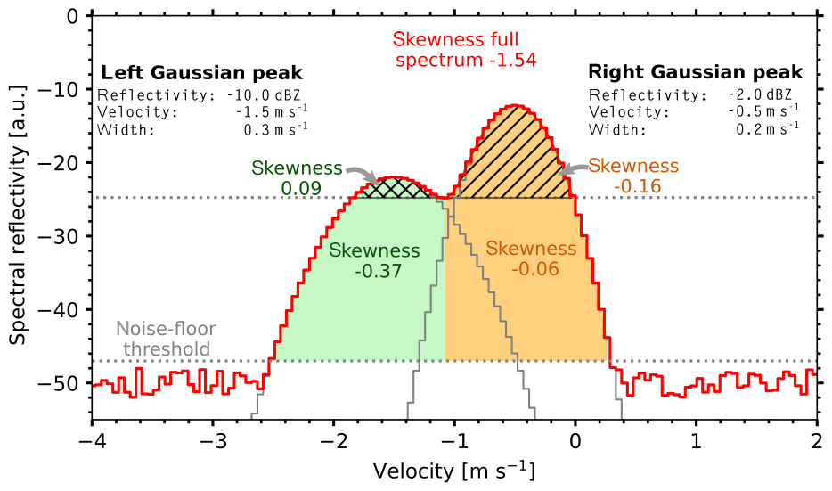
Figure A1Example for different skewness values if the spectrum is cut at the local minimum or not.
MR developed the algorithm and drafted the paper. JB supported the implementation. JB and PS supervised the work together. PS and HG preprocessed the Doppler spectra of MIRA-35. HG, RE and MR operated MIRA-35 onboard Polarstern. All authors jointly contributed to the paper and the scientific discussion.
The authors declare that they have no conflict of interest.
This article is part of the special issue “Arctic mixed-phase clouds as studied during the ACLOUD/PASCAL campaigns in the framework of (AC)3 (ACP/AMT inter-journal SI)”. It is not associated with a conference.
The research leading to these results has received funding from the European Union’s Horizon 2020 research and innovation program under grant agreement no. 654109 (ACTRIS) and the European Union Seventh Framework Programme (FP7/2007-2013) under grant agreement no. 603445 (BACCHUS). We also acknowledge the funding by the Deutsche Forschungsgemeinschaft (DFG, German Research Foundation) – project number 268020496 – TRR 172, within the Transregional Collaborative Research Center “ ArctiC Amplification: Climate Relevant Atmospheric and SurfaCe Processes, and Feedback Mechanisms (AC)3”. We thank the Alfred Wegener Institute and the R/V Polarstern crew and captain for their support (AWI_PS106_00) as well as the ARM AMF2 and SMEAR II teams for operating the instruments during BAECC. We gratefully acknowledge the constructive comments by Max Maahn and an anonymous referee.
This research has been supported by the European Commission (grant nos. 654109 and 603445) and the Deutsche Forschungsgemeinschaft (grant no. 268020496).
The publication of this article was funded by the
Open Access Fund of the Leibniz Association.
This paper was edited by Matthew Shupe and reviewed by Maximilian Maahn and one anonymous referee.
Baumgardner, D., Abel, S. J., Axisa, D., Cotton, R., Crosier, J., Field, P., Gurganus, C., Heymsfield, A., Korolev, A., Krämer, M., Lawson, P., McFarquhar, G., Ulanowski, Z., and Um, J.: Cloud Ice Properties: In Situ Measurement Challenges, Meteor. Mon., 58, 9.1–9.23, https://doi.org/10.1175/AMSMONOGRAPHS-D-16-0011.1, 2017. a
Bharadwaj, N., Matthews, A., Nelson, D., Lindenmaier, I., Isom, B., Hardin, J., and Johnson, K.: Atmospheric Radiation Measurement (ARM) user facility, updated hourly, Ka ARM Zenith Radar (KAZRSPECCMASKGECOPOL), 2014-02-02 to 2014-02-03, ARM Mobile Facility (TMP) U. of Helsinki Research Station (SMEAR II), Hyytiala, Finland; AMF2 (M1), https://doi.org/10.5439/1025218, 2014. a
Bühl, J., Seifert, P., Myagkov, A., and Ansmann, A.: Measuring ice- and liquid-water properties in mixed-phase cloud layers at the Leipzig Cloudnet station, Atmos. Chem. Phys., 16, 10609–10620, https://doi.org/10.5194/acp-16-10609-2016, 2016. a, b
Bühl, J., Alexander, S., Crewell, S., Heymsfield, A., Kalesse, H., Khain, A., Maahn, M., Van Tricht, K., and Wendisch, M.: Remote Sensing, Meteor. Mon., 58, 10.1–10.21, https://doi.org/10.1175/AMSMONOGRAPHS-D-16-0015.1, 2017. a
Carter, D. A., Gage, K. S., Ecklund, W. L., Angevine, W. M., Johnston, P. E., Riddle, A. C., Wilson, J., and Williams, C. R.: Developments in UHF lower tropospheric wind profiling at NOAA's Aeronomy Laboratory, Radio Sci., 30, 977–1001, https://doi.org/10.1029/95RS00649, 1995. a
Clothiaux, E. E., Ackerman, T. P., Mace, G. G., Moran, K. P., Marchand, R. T., Miller, M. A., and Martner, B. E.: Objective Determination of Cloud Heights and Radar Reflectivities Using a Combination of Active Remote Sensors at the ARM CART Sites, J. Appl. Meteorol., 39, 645–665, https://doi.org/10.1175/1520-0450(2000)039<0645:ODOCHA>2.0.CO;2, 2000. a, b
Doviak, R. J. and Zrnic, D. S.: Doppler Radar & Weather Observations, Courier Corporation, Academic Press, San Diego, https://doi.org/10.1016/C2009-0-22358-0, 1993. a
Engelmann, R., Kanitz, T., Baars, H., Heese, B., Althausen, D., Skupin, A., Wandinger, U., Komppula, M., Stachlewska, I. S., Amiridis, V., Marinou, E., Mattis, I., Linné, H., and Ansmann, A.: The automated multiwavelength Raman polarization and water-vapor lidar PollyXT: the neXT generation, Atmos. Meas. Tech., 9, 1767–1784, https://doi.org/10.5194/amt-9-1767-2016, 2016. a
Fan, J., Ghan, S., Ovchinnikov, M., Liu, X., Rasch, P. J., and Korolev, A.: Representation of Arctic mixed-phase clouds and the Wegener-Bergeron-Findeisen process in climate models: Perspectives from a cloud-resolving study, J. Geophys. Res.-Atmos., 116, D1, https://doi.org/10.1029/2010JD015375, 2011. a
Frisch, A. S., Fairall, C. W., and Snider, J. B.: Measurement of Stratus Cloud and Drizzle Parameters in ASTEX with a Ka-Band Doppler Radar and a Microwave Radiometer, J. Atmos. Sci., 52, 2788–2799, https://doi.org/10.1175/1520-0469(1995)052<2788:MOSCAD>2.0.CO;2, 1995. a, b
Fukao, S. and Hamazu, K.: Radar for Meteorological and Atmospheric Observations, Springer, Tokyo, https://doi.org/10.1007/978-4-431-54334-3, 2014. a
Garnier, R. and Taylor, J.: Discrete Mathematics: Proofs, Structures and Applications, Third Edition, CRC Press, Hoboken, 2009. a
Görsdorf, U., Lehmann, V., Bauer-Pfundstein, M., Peters, G., Vavriv, D., Vinogradov, V., and Volkov, V.: A 35-GHz Polarimetric Doppler Radar for Long-Term Observations of Cloud Parameters – Description of System and Data Processing, J. Atmos. Ocean. Tech., 32, 675–690, https://doi.org/10.1175/JTECH-D-14-00066.1, 2015. a, b, c
Hogan, R. J., Mittermaier, M. P., and Illingworth, A. J.: The Retrieval of Ice Water Content from Radar Reflectivity Factor and Temperature and Its Use in Evaluating a Mesoscale Model, J. Appl. Meteorol. Climatol., 45, 301–317, https://doi.org/10.1175/JAM2340.1, 2006. a, b
Illingworth, A. J., Hogan, R. J., O'Connor, E. J., Bouniol, D., Delanoë, J., Pelon, J., Protat, A., Brooks, M. E., Gaussiat, N., Wilson, D. R., Donovan, D. P., Baltink, H. K., van Zadelhoff, G.-J., Eastment, J. D., Goddard, J. W. F., Wrench, C. L., Haeffelin, M., Krasnov, O. A., Russchenberg, H. W. J., Piriou, J.-M., Vinit, F., Seifert, A., Tompkins, A. M., and Willén, U.: Cloudnet: Continuous Evaluation of Cloud Profiles in Seven Operational Models Using Ground-Based Observations, B. Am. Meteorol. Soc., 88, 883–898, https://doi.org/10.1175/BAMS-88-6-883, 2007. a
Kalesse, H., Szyrmer, W., Kneifel, S., Kollias, P., and Luke, E.: Fingerprints of a riming event on cloud radar Doppler spectra: observations and modeling, Atmos. Chem. Phys., 16, 2997–3012, https://doi.org/10.5194/acp-16-2997-2016, 2016. a, b, c, d
Kalesse, H., Vogl, T., Paduraru, C., and Luke, E.: Development and validation of a supervised machine learning radar Doppler spectra peak-finding algorithm, Atmos. Meas. Tech., 12, 4591–4617, https://doi.org/10.5194/amt-12-4591-2019, 2019. a, b
Klepp, C., Michel, S., Protat, A., Burdanowitz, J., Albern, N., Kähnert, M., Dahl, A., Louf, V., Bakan, S., and Buehler, S. A.: OceanRAIN, a new in-situ shipboard global ocean surface-reference dataset of all water cycle components, Sci. Data, 5, 180122, https://doi.org/10.1038/sdata.2018.122, 2018. a
Kogan, Z. N., Mechem, D. B., and Kogan, Y. L.: Assessment of variability in continental low stratiform clouds based on observations of radar reflectivity, J. Geophys. Res.-Atmos., 110, D18, https://doi.org/10.1029/2005JD006158, 2005. a
Kollias, P., Clothiaux, E. E., Miller, M. A., Albrecht, B. A., Stephens, G. L., and Ackerman, T. P.: Millimeter-Wavelength Radars: New Frontier in Atmospheric Cloud and Precipitation Research, B. Am. Meteor. Soc., 88, 1608–1624, https://doi.org/10.1175/BAMS-88-10-1608, 2007a. a
Kollias, P., Miller, M. A., Luke, E. P., Johnson, K. L., Clothiaux, E. E., Moran, K. P., Widener, K. B., and Albrecht, B. A.: The Atmospheric Radiation Measurement Program Cloud Profiling Radars: Second-Generation Sampling Strategies, Processing, and Cloud Data Products, J. Atmos. Ocean. Tech., 24, 1199–1214, https://doi.org/10.1175/JTECH2033.1, 2007b. a
Kollias, P., Clothiaux, E. E., Ackerman, T. P., Albrecht, B. A., Widener, K. B., Moran, K. P., Luke, E. P., Johnson, K. L., Bharadwaj, N., Mead, J. B., Miller, M. A., Verlinde, J., Marchand, R. T., and Mace, G. G.: Development and Applications of ARM Millimeter-Wavelength Cloud Radars, Meteor. Mon., 57, 17.1–17.19, https://doi.org/10.1175/AMSMONOGRAPHS-D-15-0037.1, 2016. a, b
Korolev, A., McFarquhar, G., Field, P. R., Franklin, C., Lawson, P., Wang, Z., Williams, E., Abel, S. J., Axisa, D., Borrmann, S., Crosier, J., Fugal, J., Krämer, M., Lohmann, U., Schlenczek, O., Schnaiter, M., and Wendisch, M.: Mixed-Phase Clouds: Progress and Challenges, Meteor. Mon., 58, 5.1–5.50, https://doi.org/10.1175/AMSMONOGRAPHS-D-17-0001.1, 2017. a
Luke, E. P. and Kollias, P.: Separating Cloud and Drizzle Radar Moments during Precipitation Onset Using Doppler Spectra, J. Atmos. Ocean. Tech., 30, 1656–1671, https://doi.org/10.1175/JTECH-D-11-00195.1, 2013. a
Luke, E. P., Kollias, P., Johnson, K. L., and Clothiaux, E. E.: A Technique for the Automatic Detection of Insect Clutter in Cloud Radar Returns, J. Atmos. Ocean. Tech., 25, 1498–1513, https://doi.org/10.1175/2007JTECHA953.1, 2008. a
Luke, E. P., Kollias, P., and Shupe, M. D.: Detection of supercooled liquid in mixed-phase clouds using radar Doppler spectra, J. Geophys. Res., 115, D19, https://doi.org/10.1029/2009JD012884, 2010. a, b
Maahn, M. and Löhnert, U.: Potential of Higher-Order Moments and Slopes of the Radar Doppler Spectrum for Retrieving Microphysical and Kinematic Properties of Arctic Ice Clouds, J. Appl. Meteorol. Climatol., 56, 263–282, https://doi.org/10.1175/JAMC-D-16-0020.1, 2017. a
Matrosov, S. Y. and Kropfli, R. A.: Cirrus Cloud Studies with Elliptically Polarized Ka-band Radar Signals: A Suggested Approach, J. Atmos. Ocean. Tech., 10, 684–692, https://doi.org/10.1175/1520-0426(1993)010<0684:CCSWEP>2.0.CO;2, 1993. a
Myagkov, A., Seifert, P., Wandinger, U., Bauer-Pfundstein, M., and Matrosov, S. Y.: Effects of Antenna Patterns on Cloud Radar Polarimetric Measurements, J. Atmos. Ocean. Tech., 32, 1813–1828, https://doi.org/10.1175/JTECH-D-15-0045.1, 2015. a
Myagkov, A., Seifert, P., Wandinger, U., Bühl, J., and Engelmann, R.: Relationship between temperature and apparent shape of pristine ice crystals derived from polarimetric cloud radar observations during the ACCEPT campaign, Atmos. Meas. Tech., 9, 3739–3754, https://doi.org/10.5194/amt-9-3739-2016, 2016. a, b
Oue, M., Kollias, P., Ryzhkov, A., and Luke, E. P.: Toward Exploring the Synergy Between Cloud Radar Polarimetry and Doppler Spectral Analysis in Deep Cold Precipitating Systems in the Arctic, J. Geophys. Res.-Atmos., 123, 2797–2815, https://doi.org/10.1002/2017JD027717, 2018. a, b, c, d
Petäjä, T., O’Connor, E. J., Moisseev, D., Sinclair, V. A., Manninen, A. J., Väänänen, R., von Lerber, A., Thornton, J. A., Nicoll, K., Petersen, W., Chandrasekar, V., Smith, J. N., Winkler, P. M., Krüger, O., Hakola, H., Timonen, H., Brus, D., Laurila, T., Asmi, E., Riekkola, M.-L., Mona, L., Massoli, P., Engelmann, R., Komppula, M., Wang, J., Kuang, C., Bäck, J., Virtanen, A., Levula, J., Ritsche, M., and Hickmon, N.: BAECC: A Field Campaign to Elucidate the Impact of Biogenic Aerosols on Clouds and Climate, B. Am. Meteor. Soc., 97, 1909–1928, https://doi.org/10.1175/BAMS-D-14-00199.1, 2016. a
Pfitzenmaier, L., Dufournet, Y., Unal, C. M. H., and Russchenberg, H. W. J.: Retrieving Fall Streaks within Cloud Systems Using Doppler Radar, J. Atmos. Ocean. Tech., 34, 905–920, https://doi.org/10.1175/JTECH-D-16-0117.1, 2017. a
Radenz, M., Bühl, J., Lehmann, V., Görsdorf, U., and Leinweber, R.: Combining cloud radar and radar wind profiler for a value added estimate of vertical air motion and particle terminal velocity within clouds, Atmos. Meas. Tech., 11, 5925–5940, https://doi.org/10.5194/amt-11-5925-2018, 2018. a
Radenz, M., Bühl, J., and Seifert, P.: peakTree version of Aug2019, https://doi.org/10.5281/zenodo.2577387, 2019. a
Rambukkange, M. P., Verlinde, J., Eloranta, E. W., Flynn, C. J., and Clothiaux, E. E.: Using Doppler Spectra to Separate Hydrometeor Populations and Analyze Ice Precipitation in Multilayered Mixed-Phase Clouds, IEEE Geosci. Remote Sens. Lett., 8, 108–112, https://doi.org/10.1109/LGRS.2010.2052781, 2011. a, b, c
Rose, T., Crewell, S., Löhnert, U., and Simmer, C.: A network suitable microwave radiometer for operational monitoring of the cloudy atmosphere, Atmos. Res., 75, 183–200, 2005. a, b
Schmithüsen, H.: Upper air soundings during POLARSTERN cruise PS106.2 (ARK-XXXI/1.2), https://doi.org/10.1594/PANGAEA.882843, 2017. a, b, c
Shupe, M. D., Uttal, T., Matrosov, S. Y., and Frisch, A. S.: Cloud water contents and hydrometeor sizes during the FIRE Arctic Clouds Experiment, J. Geophys. Res.-Atmos., 106, 15015–15028, https://doi.org/10.1029/2000JD900476, 2001. a
Shupe, M. D., Kollias, P., Matrosov, S. Y., and Schneider, T. L.: Deriving Mixed-Phase Cloud Properties from Doppler Radar Spectra, J. Atmos. Ocean. Tech., 21, 660–670, https://doi.org/10.1175/1520-0426(2004)021<0660:DMCPFD>2.0.CO;2, 2004. a, b, c, d
Shupe, M. D., Comstock, J. M., Turner, D. D., and Mace, G. G.: Cloud Property Retrievals in the ARM Program, Meteor. Mon., 57, 19.1–19.20, https://doi.org/10.1175/AMSMONOGRAPHS-D-15-0030.1, 2016. a
Verlinde, J., Rambukkange, M. P., Clothiaux, E. E., McFarquhar, G. M., and Eloranta, E. W.: Arctic multilayered, mixed-phase cloud processes revealed in millimeter-wave cloud radar Doppler spectra, J. Geophys. Res.-Atmos., 118, 199–213, https://doi.org/10.1002/2013JD020183, 2013. a
Wakasugi, K., Mizutano, M., Matsuo, M., Fukao, S., and Kato, S.: A direct method of deriving drop size distribution and vertical air velocities from VHF Doppler radar spectra, J. Atmos. Ocean. Tech., 3, 623–629, https://doi.org/10.1175/1520-0426(1986)003<0623:ADMFDD>2.0.CO;2, 1986. a
Wang, Z. and Sassen, K.: Cirrus Cloud Microphysical Property Retrieval Using Lidar and Radar Measurements, Part I: Algorithm Description and Comparison with In Situ Data, J. Appl. Meteorol., 41, 218–229, https://doi.org/10.1175/1520-0450(2002)041<0218:CCMPRU>2.0.CO;2, 2002. a
Wang, Z., Sassen, K., Whiteman, D. N., and Demoz, B. B.: Studying Altocumulus with Ice Virga Using Ground-Based Active and Passive Remote Sensors, J. Appl. Meteorol., 43, 449–460, https://doi.org/10.1175/1520-0450(2004)043<0449:SAWIVU>2.0.CO;2, 2004. a
Wendisch, M., Macke, A., Ehrlich, A., Lüpkes, C., Mech, M., Chechin, D., Dethloff, K., Barientos, C., Bozem, H., Brückner, M., Clemen, H.-C., Crewell, S., Donth, T., Dupuy, R., Ebell, K., Egerer, U., Engelmann, R., Engler, C., Eppers, O., Gehrmann, M., Gong, X., Gottschalk, M., Gourbeyre, C., Griesche, H., Hartmann, J., Hartmann, M., Heinold, B., Herber, A., Herrmann, H., Heygster, G., Hoor, P., Jafariserajehlou, S., Jäkel, E., Järvinen, E., Jourdan, O., Kästner, U., Kecorius, S., Knudsen, E. M., Köllner, F., Kretzschmar, J., Lelli, L., Leroy, D., Maturilli, M., Mei, L., Mertes, S., Mioche, G., Neuber, R., Nicolaus, M., Nomokonova, T., Notholt, J., Palm, M., van Pinxteren, M., Quaas, J., Richter, P., Ruiz-Donoso, E., Schäfer, M., Schmieder, K., Schnaiter, M., Schneider, J., Schwarzenböck, A., Seifert, P., Shupe, M. D., Siebert, H., Spreen, G., Stapf, J., Stratmann, F., Vogl, T., Welti, A., Wex, H., Wiedensohler, A., Zanatta, M., and Zeppenfeld, S.: The Arctic Cloud Puzzle: Using ACLOUD/PASCAL Multi-Platform Observations to Unravel the Role of Clouds and Aerosol Particles in Arctic Amplification, B. Am. Meteor. Soc., 100, 841–871, https://doi.org/10.1175/BAMS-D-18-0072.1, 2019. a
Williams, C. R., Maahn, M., Hardin, J. C., and de Boer, G.: Clutter mitigation, multiple peaks, and high-order spectral moments in 35 GHz vertically pointing radar velocity spectra, Atmos. Meas. Tech., 11, 4963–4980, https://doi.org/10.5194/amt-11-4963-2018, 2018. a, b
Yu, G., Verlinde, J., Clothiaux, E. E., and Chen, Y.-S.: Mixed-phase cloud phase partitioning using millimeter wavelength cloud radar Doppler velocity spectra, J. Geophys. Res.-Atmos., 119, 7556–7576, https://doi.org/10.1002/2013JD021182, 2014. a, b, c, d
Zhao, C., Xie, S., Klein, S. A., Protat, A., Shupe, M. D., McFarlane, S. A., Comstock, J. M., Delanoë, J., Deng, M., Dunn, M., Hogan, R. J., Huang, D., Jensen, M. P., Mace, G. G., McCoy, R., O'Connor, E. J., Turner, D. D., and Wang, Z.: Toward understanding of differences in current cloud retrievals of ARM ground-based measurements, J. Geophys. Res.-Atmos., 117, D10, https://doi.org/10.1029/2011JD016792, 2012. a