the Creative Commons Attribution 4.0 License.
the Creative Commons Attribution 4.0 License.
 | 23 Sep 2019
The impact of neglecting ice phase on cloud optical depth retrievals from AERONET cloud mode observations
Jonathan K. P. Shonk
Jui-Yuan Christine Chiu
Alexander Marshak
David M. Giles
Chiung-Huei Huang
Gerald G. Mace
Sally Benson
Ilya Slutsker
Brent N. Holben
Clouds present many challenges to climate modelling. To develop and verify the parameterisations needed to allow climate models to represent cloud structure and processes, there is a need for high-quality observations of cloud optical depth from locations around the world. Retrievals of cloud optical depth are obtainable from radiances measured by Aerosol Robotic Network (AERONET) radiometers in “cloud mode” using a two-wavelength retrieval method. However, the method is unable to detect cloud phase, and hence assumes that all of the cloud in a profile is liquid. This assumption has the potential to introduce errors into long-term statistics of retrieved optical depth for clouds that also contain ice. Using a set of idealised cloud profiles we find that, for optical depths above 20, the fractional error in retrieved optical depth is a linear function of the fraction of the optical depth that is due to the presence of ice cloud (“ice fraction”). Clouds that are entirely ice have positive errors with magnitudes of the order of 55 % to 70 %. We derive a simple linear equation that can be used as a correction at AERONET sites where ice fraction can be independently estimated.
Using this linear equation, we estimate the magnitude of the error for a set of cloud profiles from five sites of the Atmospheric Radiation Measurement programme. The dataset contains separate retrievals of ice and liquid retrievals; hence ice fraction can be estimated. The magnitude of the error at each location was related to the relative frequencies of occurrence in thick frontal cloud at the mid-latitude sites and of deep convection at the tropical sites – that is, of deep cloud containing both ice and liquid particles. The long-term mean optical depth error at the five locations spans the range 2–4, which we show to be small enough to allow calculation of top-of-atmosphere flux to within 10 % and surface flux to about 15 %.


Clouds are a crucial part of the climate system, yet present many great challenges to climate science (Randall et al., 2007; Boucher et al., 2013). Despite recent progress, climate models struggle to represent the optical properties of clouds (Bender et al., 2006; Lauer and Hamilton, 2013; Klein et al., 2013; Calisto et al., 2014). Cloud optical depth is particularly important to represent reliably as it governs the effect of clouds on the Earth's radiation budget. The complex processes and interactions that describe the evolution of clouds occur on scales much smaller than a model grid box and hence require parameterisation (Pincus et al., 2003; Shonk and Hogan, 2010). To develop and validate these parameterisations, there is a need for global observations of cloud optical depth at high temporal and spatial resolution.
A common approach to measure cloud optical depth is to retrieve it remotely from measurements of reflectance, radiance or irradiance in multiple spectral bands. Various methods have been developed to retrieve cloud optical depth from satellite measurements (for example, Arking and Childs, 1985; Nakajima and King, 1990; Platnick et al., 2001; Cooper et al., 2007) and ground-based instruments (Marshak et al., 2000, 2004; Barker and Marshak, 2001; Chiu et al., 2006). The need for global observations is best met by satellites, which are capable of providing routine cloud optical depth retrievals all around the world. However, on account of their large pixel size, they struggle to provide the high temporal and spatial resolution required to investigate cloud processes. The underlying surface adds to the complexity of variability in the optical properties, and broken clouds and subpixel clouds increase the chance of errors and biases (Stephens and Kummerow, 2007). Using ground-based observations eliminates many of these issues. The proximity of clouds to the ground (much closer than a satellite orbit) means that a radiometer can achieve much smaller pixel sizes for the same viewing angle, allowing much higher temporal and spatial resolution, and reducing the incidences of cloud edge.
A disadvantage of using ground-based observations is the lack of global coverage. We are limited to the small number of locations around the world where routine cloud optical depth observations are made: until recently, sites of the Atmospheric Radiation Measurement (ARM) programme (Stokes and Schwartz, 1994) and the sites of the Aerosols, Clouds and Trace Gases Research Infrastructure (ACTRIS) network that were formerly part of Cloudnet (Illingworth et al., 2007). But Chiu et al. (2010) noted that radiometers distributed throughout the world as part of the AERONET project (Holben et al., 1998) could provide a readily available source of cloud optical depth observations and hence provide greater global coverage. When the sun is not obscured by cloud, these radiometers are in “aerosol mode” and make regular measurements of aerosol properties. When the sun is obscured, however, aerosol measurements are not possible and the radiometer becomes idle. Marshak et al. (2004) proposed that the “downtime” when the aerosol measurements are not possible could be used to observe cloud properties (“cloud mode”) via measurements of zenith radiance.
Cloud optical depth retrievals are performed using the method proposed by Chiu et al. (2010). It is based on that of Marshak et al. (2004), and uses zenith radiances measured at two wavelengths (440 and 870 nm; one visible, one infra-red) to retrieve cloud optical depth and cloud fraction. Above a green, vegetated surface, the radiative properties of the clouds are similar at these wavelengths, but there is a strong contrast in surface albedo. Retrieval is performed using a set of radiance look-up tables calculated at the two wavelengths. The approach has been shown to be applicable for both overcast and broken cloud fields (Chiu et al., 2006), and performed well when applied to an artificial field of clouds whose optical depth was known (Marshak et al., 2004). A limitation to the method is that it does not perform well near cloud edge: clear-sky contamination of the field of view and high radiances arising from direct solar illumination of cloud edge can both generate unrealistic optical depths (Chiu et al., 2006). In AERONET, contamination problems are reduced by clustering retrievals into 1.5 min intervals and excluding extreme optical depth values (Chiu et al., 2010).
Using this method, AERONET cloud mode optical depth retrievals have now been carried out routinely at a number of sites around the world for several years. A requirement for a cloud mode site is that the surrounding area is generally green vegetation: suitable AERONET sites were selected using satellite-derived contrasts in albedo at the two wavelengths (Chiu et al., 2010). Cloud mode retrievals from AERONET are beginning to appear in published studies. An evaluation of data from one AERONET site in Cuba was performed by Barja et al. (2012). Antón et al. (2012) used cloud mode data in a study into the effects of cloud optical depth on the transmission of ultraviolet radiation; Li et al. (2019) used cloud mode data to investigate seasonal and spatial distributions of cloud optical depth across China alongside satellite optical depth retrievals from MODIS (the Moderate Resolution Imaging Spectroradiometer; Platnick et al., 2003). An AERONET radiometer was also taken aboard a ship to probe the properties of boundary layer cloud in the north-eastern tropical Pacific (Painemal et al., 2017).
An extension to the retrieval method by Chiu et al. (2012) included a third wavelength (1640 nm), which allows a retrieval of cloud droplet effective radius to be obtained alongside cloud optical depth and cloud fraction. Effective radius retrievals tend to be very sensitive to uncertainty in surface albedo and radiance measurements, so Chiu et al. (2012) suggested performing the retrieval 40 times with perturbations to surface albedo and the measured radiance, thereby providing mean values of the retrieved values and an estimate of the uncertainty in these retrievals. This method was used in the study of Painemal et al. (2017), although the standard retrievals available on the AERONET website use the two-wavelength method of Chiu et al. (2010).
However, neither of these retrieval methods are capable of retrieving cloud phase, so an assumption is made. Given the tendency for the liquid component of a cloudy profile to be substantially optically thicker than the ice component, it is assumed that the entirety of the retrieved cloud optical depth value is due to the presence of liquid cloud. This “warm cloud assumption” has the potential, therefore, to introduce an error into cloud optical depth retrievals in any case where a cloudy profile contains ice cloud, which could cause problems in studies that analyse long-term statistics of cloud optical depth.
The objectives of this study are to (1) investigate the magnitude and sign of the retrieval error due to the warm cloud assumption, (2) ascertain whether it is large enough to drastically affect the statistics of long-term optical depth retrievals and, if necessary, (3) discover whether a simple correction method could be used to account for the error. The next section of this paper describes the Chiu et al. (2010) retrieval method in more detail and provides a first estimate of the sign and magnitude of the error. In Sect. 3, we examine the relationship of the error with both total cloud optical depth and how the optical depth is partitioned between ice and liquid components by performing retrievals on a set of idealised cloud profiles. From these results, we propose a simple linear correction equation that could be employed in AERONET locations where ice fraction can be independently determined. In Sect. 4, we investigate the potential magnitude of the error in real clouds measured at five ARM sites using retrieval methods described by Mace et al. (2006). We then discuss the results in Sect. 5 and then summarise the study in Sect. 6.
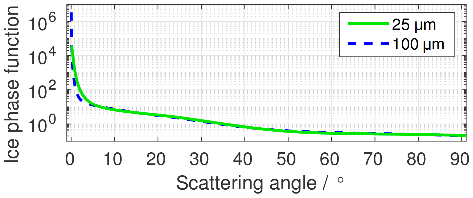
Figure 1Ice phase functions used in this study, originally designed for use in cloud retrievals from MODIS. Phase functions are shown for the forward scattering direction at wavelength 465 nm, for two ice particle effective diameters (see legend).
Retrievals throughout this study are performed using the two-channel method described by Chiu et al. (2010). The method begins with a set of look-up tables, which contain the radiance that would be observed at the surface under a cloudy profile for a range of different cloud optical depths, solar zenith angles and values of droplet effective radius. Using the Discrete Ordinate Method for Radiative Transfer radiation code (DISORT; Stamnes et al., 1988), a set of tables is calculated for each of the two wavelength channels, 440 and 870 nm. The surface albedo in the two channels is set to 0.05 and 0.35 respectively (typical albedo values over a green vegetated surface as reported by Chiu et al., 2010). The scattering properties applied to DISORT for all look-up table calculations are those of liquid water droplets. The look-up tables span the optical depth range 1 to 100.
A pair of measured radiances at the two wavelengths is fed into the retrieval algorithm along with an assumed liquid effective radius (taken to be 8 µm throughout this study) and the known solar zenith angle at that time. From the look-up tables, the algorithm then searches for values of optical depth and cloud fraction that produce the specified radiances at the two wavelengths. To estimate the uncertainty on the retrieval, we follow part of the method of Chiu et al. (2012) and perform 40 calculations, each one with a random perturbation applied to both the surface albedos and the observed radiances to represent uncertainty in their measurement. The output retrieved optical depth and cloud fraction therefore consist of a mean value and an indication of uncertainty.
To make an initial estimate of the sign and magnitude of the “warm cloud error”, we use DISORT to calculate a few look-up tables using scattering properties of ice particles and compare them with the corresponding look-up tables calculated using the properties of liquid droplets. We use a set of ice crystal phase functions for a randomly aligned distribution of rough-surfaced ice crystals, consisting of a mixture of shapes (a “general habit mixture”), retrieved from https://www.ssec.wisc.edu/ice_models/ (last access: 25 October 2018). These phase functions were calculated alongside other single-scattering properties from field campaign data by Baum et al. (2011, 2014). Their calculated properties are designed for use with radiative transfer calculations that allow retrieval of optical properties from satellites, with a different set of properties for each satellite platform to allow consistent retrieval. Given the availability of phase functions near the two wavelengths used in AERONET cloud optical depth retrievals, we select the phase functions designed for MODIS. Figure 1 shows the ice phase functions at wavelength 465 nm for particles with effective diameters of 25 and 100 µm (the range of effective diameters that we consider in this study). The corresponding phase functions at 855 nm are similar.

Figure 2Normalised radiances extracted from the liquid (red) and ice (blue and green) look-up tables for a range of different optical depths, all calculated with unit top-of-atmosphere flux, for a solar zenith angle of 30∘ and at the visible 440 nm wavelength over a surface albedo of 0.05. The numbers in the legend are values of liquid effective radius and ice effective diameter.
Figure 2 compares the radiances that would be observed at the surface at the respective visible wavelengths under a column of cloud that is either purely ice or purely liquid, for a prescribed solar zenith angle of 30∘ and a top-of-atmosphere flux of unity (hence the radiances presented are normalised). For a given optical depth, the observed radiance for liquid clouds is always more than that for an ice cloud of the same optical depth over the entire range of effective sizes used in this study. This is because liquid droplets have a greater tendency to forward scatter than ice crystals, resulting in a greater radiance at the surface for the same amount of extinction. For any profile whose true optical depth is in the branch of the curve in Fig. 2 where the radiance is monotonically decreasing with increasing optical depth (that is, to the right of the maximum), the error in retrieved cloud optical depth will be positive. Consider an example: the observed normalised radiance is 0.4, and we assume that the cloud is liquid with an effective radius of 8 µm and has an optical depth greater than 10. From Fig. 2, we would retrieve an optical depth of about 25. However, if all of the cloud is in fact rough ice crystals with an effective diameter between 25 and 100 µm, the actual optical depth might only be between 16 and 17, implying a positive error of between 47 % and 56 %.
For a better understanding of the retrieval error, we use the two-channel retrieval method to obtain cloud optical depth for a set of idealised cloud profiles where the cloud optical depth is known. Each profile includes two cloudy layers: the top layer is filled with ice cloud and the bottom layer is filled with liquid cloud, both with a cloud fraction of 1. The properties of these cloud layers are varied in two ways. First, the total combined optical depth of the two layers is varied. Second, the partitioning of this total column optical depth between the ice and liquid layer is varied. We define a variable called “ice fraction” – this is the fraction of the total column optical depth that is due to the presence of ice cloud. For each combination of optical depth and ice fraction, a full radiative transfer calculation is performed using DISORT to obtain the zenith radiance that would be detected at the surface by a vertically pointing radiometer, serving as the synthetic observed radiance. The appropriate scattering properties are used for the liquid and ice layers. We fix liquid effective radius at 8 µm, and perform radiance calculations for ice effective diameters of 25, 35, 55, and 100 µm and for solar zenith angles of 10, 30, 50 and 70∘, in both the 440 and 870 nm channels. Aerosol concentrations are set to zero.
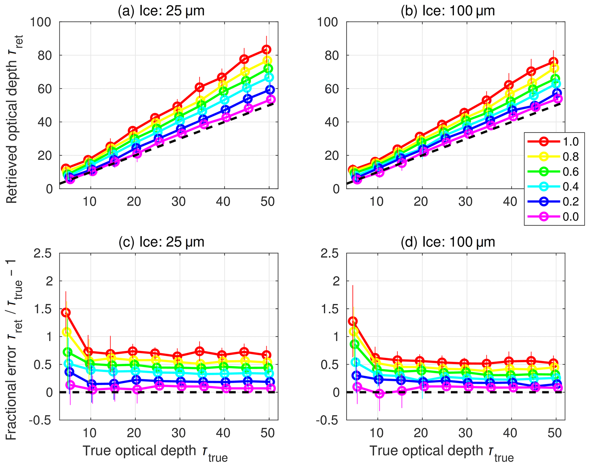
Figure 3Retrieved optical depth (τret; a, b), and retrieved optical depth as a fraction of prescribed (“true”) optical depth (Δτret∕τtrue; c, d) as a function of the true optical depth for the idealised cloud columns. Retrievals are made from DISORT radiance calculations with a liquid effective radius of 8 µm, a solar zenith angle of 30∘ and two values of ice effective diameter (see panel headers). The lines and markers are coloured according to the ice fraction (see legend). The uncertainty in the retrieval, depicted here as the standard deviation in the retrievals across the 40 samples, is indicated by the vertical bars. Note that the markers and bars for each ice fraction value are slightly horizontally offset for clarity. Black dashed lines indicate the one-to-one line in (a, b) and the zero line in (c, d).
Retrievals of cloud optical depth are then made from the observed radiances under the assumption that all clouds are liquid. Figure 3 shows that the true optical depth is generally well matched by the retrieved optical depth for profiles that contain cloud that is entirely liquid (ice fraction equal to zero), while increasing ice fraction reduces the surface radiance for a given cloud optical depth and results in an increasingly positive error. Furthermore, at most optical depths shown here, the fractional error in retrieved optical depth is largely independent of the true optical depth and increases linearly with increasing ice fraction. For clouds that are entirely ice (ice fraction equal to one), the fractional error reaches about 70 % if the ice effective diameter is assumed to be 25 µm and about 55 % if it is assumed to be 100 µm. The fractional error is also largely independent of solar zenith angle, remaining at about 70 % when the ice effective diameter is fixed at 25 µm and the solar zenith angle is varied (Fig. 4).
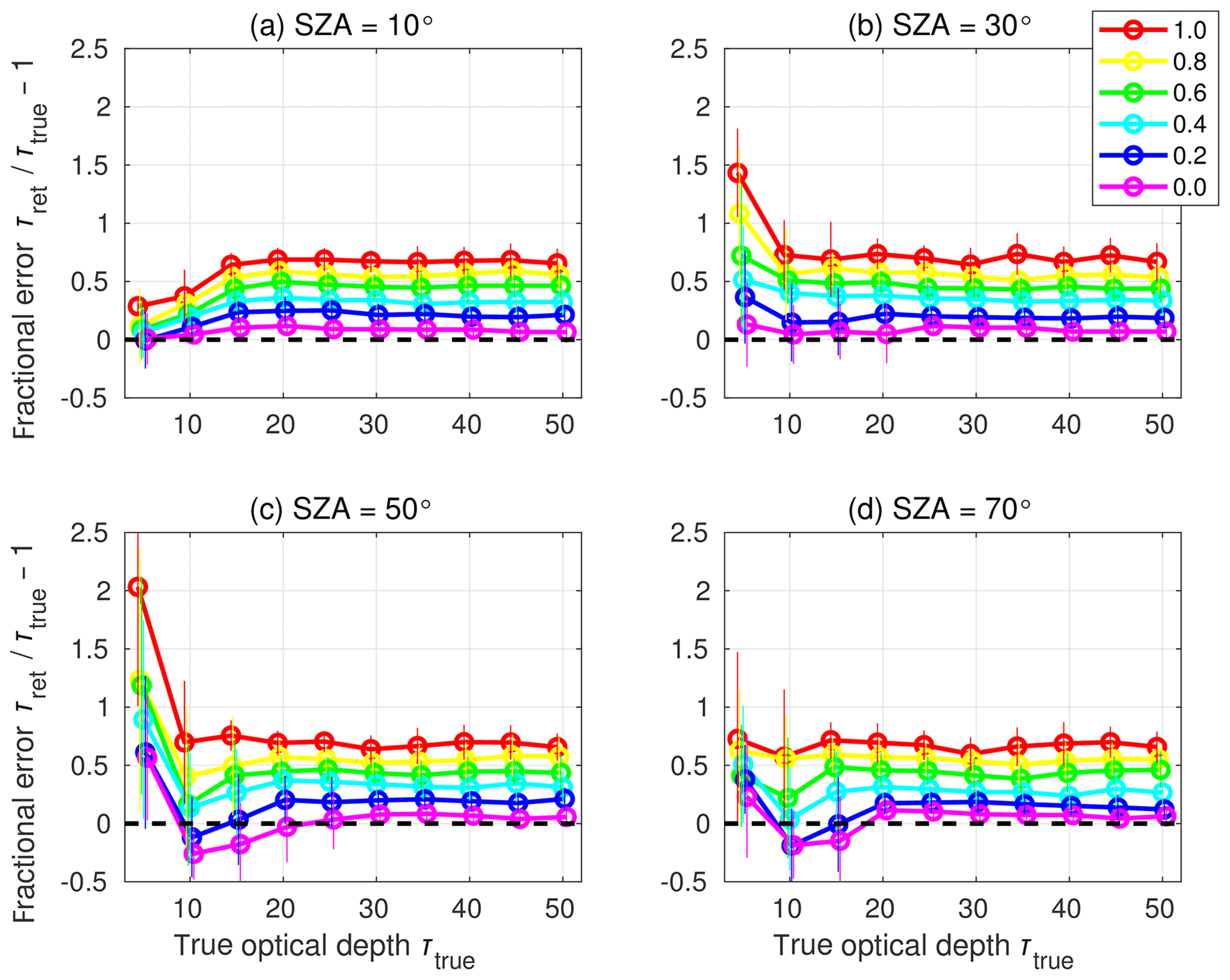
Figure 4Retrieved optical depth as a fraction of true optical depth (Δτret∕τtrue) as a function of the true optical depth in the idealised cloud columns. Retrievals are made from DISORT radiance calculations with a liquid effective radius of 8 µm, an ice effective diameter of 25 µm and four values of solar zenith angle (see panel headers). Lines and markers as described in Fig. 3.
At low optical depths (values below about 20), however, the relationship between fractional error and ice fraction becomes more complicated, with a dependence on both the true optical depth and the solar zenith angle. The range of low optical depths affected by this more complicated relationship is also dependent on solar zenith angle. A simple explanation for these two different “error regimes” arises from Fig. 2 and how the shape of the curves change with changing solar zenith angle and ice fraction. At higher optical depths (the “linear regime”), the observed radiance decreases monotonically with increasing optical depth. Changes to the ice fraction or solar zenith angle may change the nature of the curve, but do not change this monotonic behaviour. At lower optical depths (the “non-linear regime”), the change of shape does not just affect the gradients, but also the location of the maximum point of the curve, adding complicated non-linearity into the relationship.

Figure 5Fractional error in the retrieved optical depth, calculated as , for the idealised cloud columns as a function of the prescribed ice fraction (horizontal axis) and solar zenith angle (colours; see legend). The four columns of points around each 0.1 interval in ice fraction indicate the distributions of fractional error across the four values of ice effective diameter (25, 35, 55 and 100 µm from left to right). A linear fit through the points is shown (solid line), along with an estimate of its uncertainty (dashed lines).
Based on DISORT computations and the assumed ice cloud particle diameters above, the relationship between fractional error in retrieved optical depth Δτ∕τtrue and ice fraction f in the linear regime is quantified using a simple linear empirical equation of the form
where a and b are the regression coefficients, and Δa and Δb are the uncertainties in these coefficients. This regression is demonstrated in Fig. 5 and yields coefficients of a=0.534, b=0.067 and Δb=0.052. (The value of Δa was found to be negligible and less than 0.001.) To ensure retrievals in the non-linear regime are excluded, this regression only includes profiles with a true optical depth of greater than 20. To include a measure of uncertainty in the size of the ice particles, we include retrievals for all four values of ice effective diameter. Given that the solar zenith angle is known for a retrieved profile, it is conceivable to calculate regressions for each solar zenith angle separately and then add a solar zenith angle dependence to Eq. (1). However, variations in the regression coefficients for different solar zenith angles were found to be small, so we include all four solar zenith angles in one single regression for simplicity.
A simple linear equation of this form may be used to correct the warm cloud error in AERONET optical depth retrievals if an estimate of ice fraction is available at the AERONET site; for example, via separate retrievals of liquid and ice water paths from microwave radiometer and radar measurements. For all clouds in the linear regime with true optical depths of above 20, it can provide reliable correction in the range of solar zenith angles considered here. In the optical depth range 10 to 20, applying the correction equation could lead to errors in some instances of high sun or low sun, although these are likely to be small (see Fig. 4). Below optical depths of 10, the non-linear regime dominates and the reliability of the correction equation becomes questionable, as the fractional errors start to become large. However, when the values of optical depth are low, the absolute magnitude of the errors will be small and hence not a substantial contribution to errors in long-term cloud statistics. For the purposes of this study, we retain the simple linear regression presented above and accept its limitations. But we recognise that, for applications where retrievals of low optical depth are important, a more complex correction equation may be needed to account for errors in the non-linear regime. This is discussed further in Sect. 5.
For optically thick clouds with a high ice fraction, the error in retrieved optical depth can be large following Eq. (1) (for a cloud that is entirely ice and has an optical depth of 50, for example, the error is about 30). The question then follows as to how frequently such optically thick ice clouds occur at the location of the AERONET sites with cloud mode retrieval. The assumption that the liquid component of a cloudy profile tends to be optically thicker than the ice component, stated in Sect. 1, suggests that optically thick ice clouds may not be a frequent occurrence and hence only provide a small contribution to long-term statistics of cloud optical depth. In this section, we address this question by examining the distribution of optical depth and ice fraction in real clouds.
We therefore require a dataset that can provide independent values of ice and liquid components of optical depth at sites that contain AERONET radiometers that operate in cloud mode. We hence use cloud data retrieved at five ARM sites, using algorithms described by Mace et al. (2006) and hereafter referred to as “ARM Mace” data. The methods of Mace et al. (2006) derive a wealth of properties of an atmospheric profile using a combination of ground-based remote sensing techniques and radiosonde soundings, and provide a series of cloud profiles averaged over 5 min intervals with a vertical resolution of 90 m. Liquid water path is obtained from brightness temperatures measured in two wavelength channels by a microwave radiometer. Ice water content is determined from millimetre cloud radar measurements using two approaches, depending on whether the profile contains pure ice cloud or a combination of ice and liquid cloud (either in separate layers or mixed phase). The former case uses one of a set of algorithms to determine a distribution of ice water content from radar reflectivity and either Doppler velocity or longwave radiance at the surface; the latter uses a specially developed parameterisation that also uses radar reflectivity and Doppler velocity. Separate values of ice and liquid optical depth components are then calculated from the liquid water path and the vertically integrated ice water content, hence allowing an estimate of ice fraction.
Table 1A summary of cloud statistics across the five ARM sites discussed in this study. Profiles included in these statistics consist only of those from the ARM Mace dataset at times when an AERONET cloud mode retrieval would have been possible (see third and fourth paragraphs of Sect. 4 for criteria).
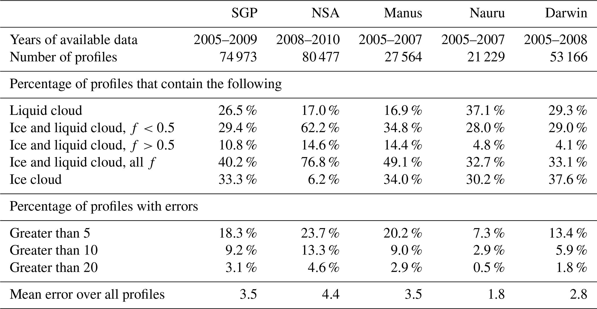
We fetched all available ARM Mace data from 2005 onwards at the Southern Great Plains site (SGP) in Oklahoma, the three Tropical Western Pacific sites in Manus, Nauru, and Darwin, and the North Slope of Alaska site (NSA) in Utqiaġvik (formerly Barrow). There are at least 3 years of data at each site, although the range of available years varies (see top part of Table 1). From these ARM Mace data, we extracted profiles that are potentially observable by an AERONET radiometer in cloud mode. We first removed all night-time profiles, and any profiles measured during periods of rainfall. Rainy profiles are indicated by the “precipitation flag” that is contained within the ARM Mace dataset; night-time profiles are identified by instances where the solar zenith angle is greater than 90∘. We also removed any profiles that contained a retrieved value of ice water content greater than 2 g m−3, as such values cannot be considered reliable according to the ARM Mace documentation.
Finally, we accounted for the upper limit of total optical depth that can be retrieved by the AERONET cloud mode algorithm by removing profiles that have a retrieved optical depth of greater than 100. Considering the ARM Mace optical depths to be the “truth”, we used Eq. (1) to simulate the AERONET cloud mode retrieval process, generating a set of “retrieved” optical depths. Any retrieved optical depths greater than 100 were excluded. The retrieval error for each profile was determined as the difference between the true and retrieved optical depth values.
It should be noted that this sample does not exclude profiles where the cloud optical depth is low, yet an AERONET aerosol mode retrieval is possible. Such a profile would be rejected from the aerosol dataset as cloud contaminated, but would also not count towards the cloud mode statistics. However, accounting for these low optical depth profiles would not be trivial. Aerosol mode retrievals can be made for aerosol optical depths of up to 5 to 7 (Giles et al., 2019), but there is no specific corresponding threshold in cloud optical depth. In the interests of ensuring the profiles that are potentially observable by AERONET in cloud mode are included, we chose to retain all low cloud optical depth profiles in the analysis, recognising that the frequency of occurrence of such profiles is likely to be overestimated.
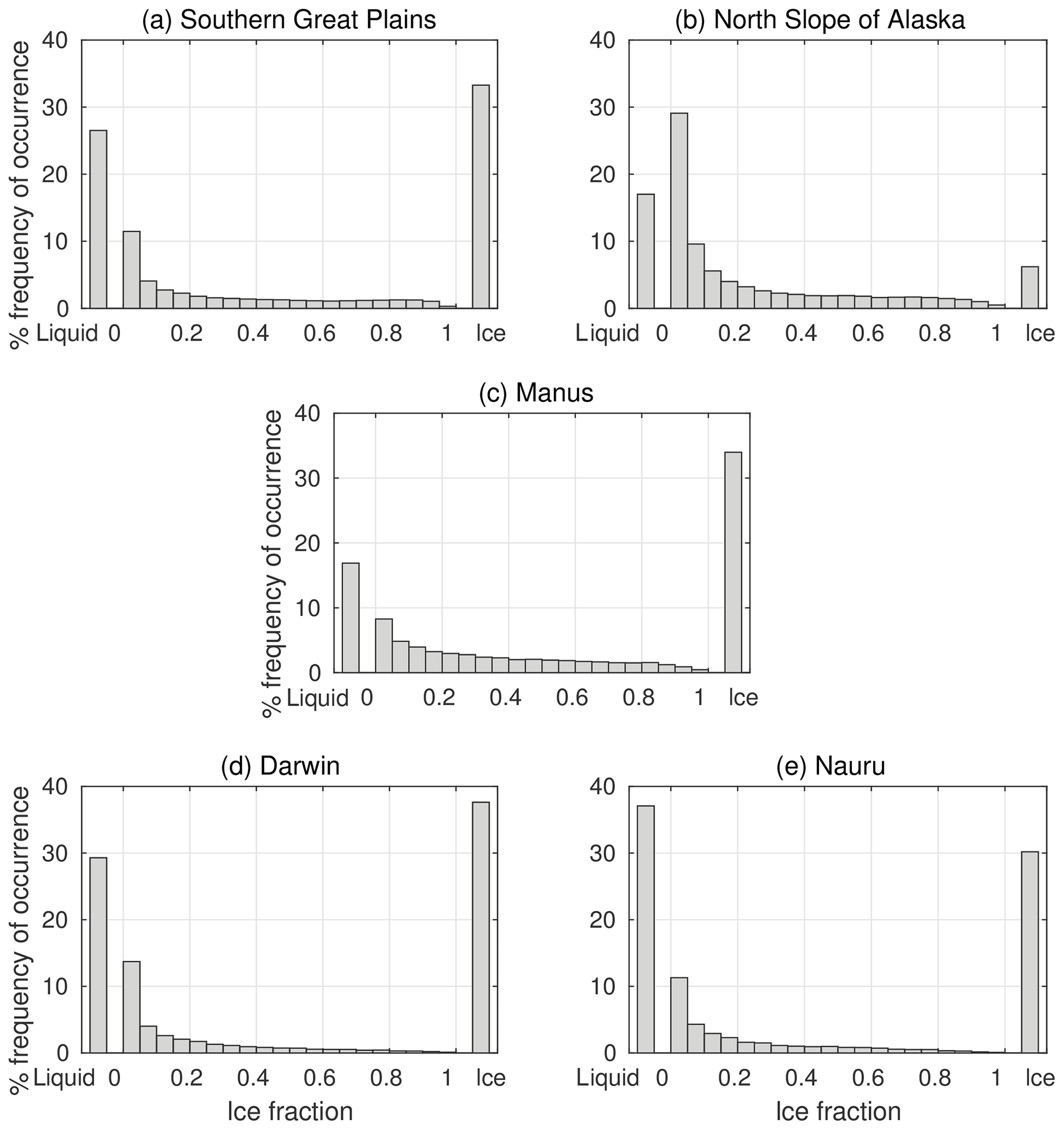
Figure 6Histograms of ice fraction for real clouds observed at five ARM sites. All available profiles in the period 2005 to 2010 are included for which an AERONET cloud mode retrieval would have been possible (see third and fourth paragraphs of Sect. 4 for conditions). The “liquid” and “ice” bars indicate the fraction of total profiles that contain purely liquid or ice; the remaining bars indicate all other profiles, separated into bins of ice fraction. Data from the Mace et al. (2006) dataset (“ARM Mace”).
We begin by analysing profiles from SGP – a mid-latitude site whose cloud regimes consist of both frontal and convective clouds with an overall average cloud fraction of about 50 % (Lazarus et al., 2000). Ice fraction for SGP profiles is shown as a histogram in Fig. 6a. Of the profiles, 26.3 % contain cloud that is purely liquid and 33.3 % contain cloud that is purely ice. Of the remaining 40.2 % that contain both liquid and ice cloud, profiles that are mostly liquid (f<0.5) outnumber those that are mostly ice (f>0.5) by about three to one.
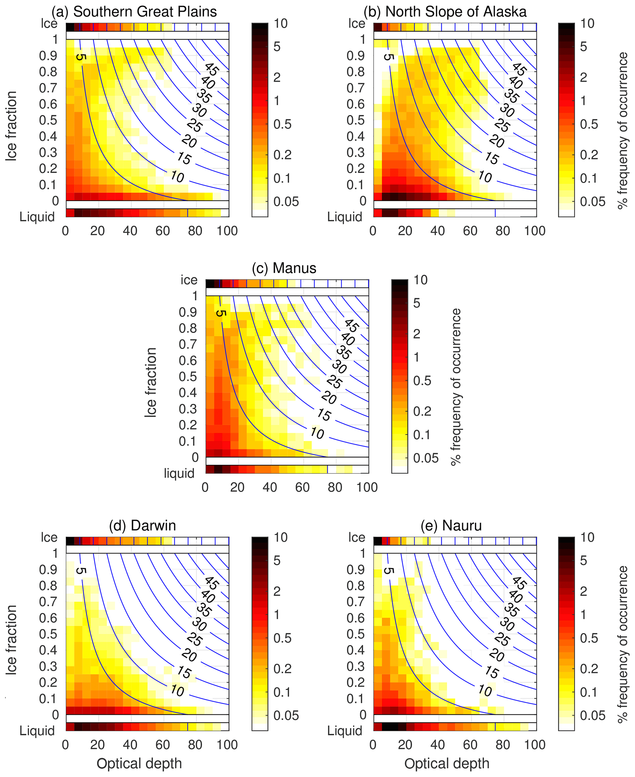
Figure 7Two-dimensional histograms of ice fraction and cloud optical depth at the five ARM sites for the same set of profiles as in Fig. 6. The “liquid” and “ice” rows show the optical depth distribution of the profiles that contain purely ice or liquid; the rest of the plot separates the mixed ice and liquid clouds by ice fraction as in Fig. 6. The colour scale indicates the fraction of the total number of profiles in each two-dimensional bin. The blue lines show the absolute error in retrieved optical depth that would result from AERONET retrievals as a function of ice fraction and cloud optical depth, calculated from Eq. (1).
Most of the profiles containing cloud that is either mostly or entirely ice have a low optical depth, and would therefore provide small contributions to long-term error statistics in a cloud optical depth climatology from AERONET (Fig. 7a). Conversely, optical depth values for liquid or mostly liquid profiles tend to be greater, but the contributions to overall mean error are also likely to be small on account of low values of ice fraction. The contours on all panels of Fig. 7 indicate the error in an AERONET retrieval as a function of optical depth and ice fraction following Eq. (1). At SGP, just under 1 in 10 of the profiles has a cloud optical depth retrieval error of greater than 10 (9.2 %), while only 3.1 % of the profiles lie in the region where the error is 20 or greater. The mean error across all profiles is 3.5.
At NSA, cloud fraction tends to be higher than SGP at about 75 % (Dong et al., 2010), consisting of mostly stratiform cloud. There is a prevalence of thick, low-level mixed-phase cloud (Mülmenstädt et al., 2012), particularly in the summer when most NSA profiles occurred (note that NSA is inside the Arctic Circle, so no AERONET profiles are possible in the perpetual darkness of winter). Table 1 shows that there is a much greater frequency of cloudy profiles containing both liquid and ice at NSA with respect to SGP, with much fewer profiles occurring that are either pure liquid or pure ice (Fig. 6b). The result is a higher frequency of optically thicker clouds that are mostly ice, but a lower frequency of optically thicker profiles that are entirely ice (Fig. 7b). The mean error in cloud optical depth as NSA is 4.4 – slightly higher than at SGP.
At the three tropical sites, the clouds tend to be much deeper and convective in nature, with a much greater occurrence of upper-level ice clouds (Stubenrauch et al., 2010). Despite their relative proximity, however, the meteorological conditions at the three sites are quite different. Manus is situated in the western Pacific “warm pool”, and experiences much more convective activity throughout the year (Jakob and Tselioudis, 2003), while Nauru is on the edge of the warm pool and experiences much less, although with a strong influence from the phase of the El Niño–Southern Oscillation (Long et al., 2013). In contrast, Darwin experiences a strong seasonal cycle in its convective activity associated with the passage of the Australian monsoon, with deep convective clouds occurring seasonally (Protat et al., 2011).
The prevalence of deep convection at the three sites reflects the differences in frequency of profiles with high ice fraction (Fig. 6c, d, e). The total frequency of profiles that contain both ice and liquid and have an ice fraction greater than 0.5 is 14.4 % at Manus, 4.8 % at Darwin and 4.1 % at Nauru. The greater frequency of convection at Manus appears as a higher fraction of profiles with high ice fractions (Fig. 7c), resulting in the greatest overall error across the tropical sites (3.5). The much lower frequency of convection at Nauru results in fewer profiles appearing in this area of the histogram (Fig. 7e), and hence a much smaller overall error (1.8). With an intermediate amount of convection and a greater fraction of optically thick ice cloud, the mean error at Darwin lies between the values at Manus and Nauru (2.8).
The analysis above from the five ARM sites implies that, if an estimate of ice fraction is not available at a given AERONET site, using uncorrected retrieved optical depths will lead to a mean error of the order of 2–4 in long-term statistics. Assuming typical mean cloud effective radius values of 6–12 µm, cloud optical depth errors of 2–4 are equivalent to errors in liquid water path of 8–32 g m−2 (using Eq. (2) in Chiu et al., 2012), which is of similar magnitude to retrieval uncertainty in liquid water path from microwave radiometer observations (Marchand et al., 2003; Crewell and Löhnert, 2003).
To compare these uncertainties to a relevant climate variable, let us set out to retrieve cloud optical depths to sufficient accuracy that both top-of-atmosphere and surface fluxes are correct to within 10 %. According to Fig. SB1 of Turner et al. (2007), for a liquid cloud with a liquid water path of 100 g m−2 and an effective radius of 8 µm, a typical top-of-atmosphere shortwave flux would be 500 W m−2 and the sensitivity of the top-of-atmosphere flux to the liquid water path would be about 1 W m−2 (g m. In this case, reproducing the top-of-atmosphere flux to within 50 W m−2 implies a need for retrieval with an error of less than 50 g m−2, equivalent to a cloud optical depth error of about 10. The mean AERONET cloud mode error of 2–4 is within this limit. By a similar argument, the presence of the same liquid cloud would result in a surface flux of about 300 W m−2 with a sensitivity of surface flux of about 2 W m−2 (g m. To get the 10 % accuracy in surface flux, the retrieval then would need to be accurate to less than about 15 g m−2 in liquid water path, or 3 in optical depth. Our errors may be slightly higher than this limit in some locations, and could only reach ∼15 % accuracy in surface flux.
At present, not all AERONET sites have the instrumentation to allow an ice fraction estimate to be made. A potential method to detect particle phase using AERONET radiometers that are polarimetrically sensitive could help with estimates of ice fraction, although further work is needed (Knobelspiesse et al., 2015). Estimates of ice fraction could be generated from other sources – for example, radiosonde soundings and satellite measurements. However, while these approaches may provide an estimate of ice fraction over a given area or timescale, they would not be capable of providing the high temporal resolution of ice fraction needed to complement the frequency of AERONET cloud mode retrievals. Further work into the applicability of such estimates would be required.
Needless to say, if an independent estimate of ice fraction is available, we advocate the use of Eq. (1) as a correction factor. Given that it is specific to the retrieval algorithm, it will be globally applicable to radiance measurements from any AERONET radiometer under the assumption that the ice crystals in a cloud are rough, consist of a mixture of shapes and have effective diameters in the range 25 to 100 µm. The equation we have proposed here is applicable for all profiles with optical depths over 20 and performs satisfactorily on profiles with optical depths from 10 to 20. While the equation presented here does not perform well for profiles with optical depths below 10, it may easily be extended to provide better correction at low optical depths via extra non-linear regressions. Alternatively, retrieval methods are being developed that allow the retrieval of low optical depths from surface radiometers: Guerrero-Rascado et al. (2013) proposed a method to obtain cloud optical depth estimates using cloud-contaminated AERONET aerosol mode observations, which could provide an alternative source of data for low cloud optical depths. The method of Hirsch et al. (2012) could also be used, although this would require the installation of specialised radiometers at AERONET sites.
Another possible extension to Eq. (1) involves the treatment of mixed-phase clouds. We generated the equation using idealised profiles with separate layers of ice and liquid cloud, therefore working under the assumption that, generally, ice and liquid cloud is separate. This fails to account for layers of mixed-phase cloud, however, which consist of a mixture of ice and liquid particles. Following Sun and Shine (1994), the zenith radiance below a mixed phase cloud will be slightly lower than that below the same cloud but with its ice and liquid particles separated into two layers. Quantifying the effect of this mixing on the correction equation would be a pertinent future step.
The representation of cloud properties in climate models still presents a huge challenge to climate scientists. To make progress in our understanding of cloud processes, we need global observations of cloud optical depth at high spatial and temporal resolution. Ground-based measurements are best suited to provide such resolution, although global coverage is limited. Using the radiometers of the Aerosol Robotic Network (AERONET) increases the number of sites around the world by making routine cloud mode measurements made during the downtime when aerosol measurements are not possible. Retrievals are made using radiance at two wavelengths (440 and 870 nm) and a set of look-up tables. However, as the method is not able to retrieve cloud phase, the assumption is made that all of the retrieved optical depth is due to the presence of warm, liquid cloud – hence, for any cloudy profile that contains an ice cloud component, there will be an error in the retrieval.
We began by investigating the sign and magnitude of this warm cloud error. A set of idealised cloud profiles were generated with varying total optical depth and ice fraction (the fraction of optical depth in the profile that is due to the presence of ice cloud). We calculated the radiances that would be observed by a radiometer at the surface underneath the cloud profiles, and then used these radiances to retrieve the cloud optical depth. Comparison of the retrieved optical depths with the true, prescribed optical depths revealed that, for profiles that are mostly or entirely ice, the fractional error in retrieved optical depth was between 55 % and 70 % for ice particle diameters between 25 and 100 µm. At optical depths of above 20, the fractional error was found to be a simple linear function of ice fraction and showed negligible dependence on optical depth or solar zenith angle. Using a simple linear regression, we were able to generate an empirical equation (Eq. 1 in this paper) linking the fractional error to the ice fraction. This equation has the potential to be used as a correction factor for AERONET optical depth retrievals. However, independent estimates of ice fraction are needed, which is currently not possible at most AERONET sites.
We then estimated the error in retrieved optical depth for a range of profiles of real clouds. We used multiple years of cloud data from five sites of the Atmospheric Radiation Measurement (ARM) programme, which were then sampled to include only profiles that could potentially be observed by an AERONET radiometer in cloud mode. Using Eq. (1), an estimate of the retrieval error was generated for each profile. Clouds that were mostly ice tended to have lower optical depths, while optically thicker clouds tended be mostly or entirely liquid – both of these conditions lead to small errors. At each of the five sites, only ∼15 % of the profiles had an error in retrieved cloud optical depth of larger than 10. The magnitude of the mean error at each location was dominated by the frequency of occurrence of optically thick clouds that were mostly or entirely ice – that is, either thick frontal cloud or deep convection. At the two sites located outside the tropics, where thick frontal cloud is the largest error contribution, the overall mean error was related to the frequency of occurrence of such optically thick clouds composed of both ice and liquid particles. In the tropics, the error at each location was related to the frequency of occurrence of deep convection, with much greater variety in the error statistics. This suggests that variations in convective cloud occurrence may have a greater influence on the overall error than variations in frontal cloud occurrence.
The mean value of optical depth retrieval error at the five ARM sites is typically in the range 2 to 4. We showed that errors of this magnitude are small enough to allow the calculation of top-of-atmosphere fluxes to within 10 % accuracy, and surface fluxes to within about 15 %. Furthermore, when expressed in terms of liquid water path, these errors are of comparable value to uncertainties in retrievals from microwave radiometers. These results alone suggest that AERONET cloud mode retrievals provide a valuable source of cloud optical depth data from a large network of surface observation sites. A higher degree of accuracy may be possible, though, via the use of a correction equation if an independent estimate of ice fraction is obtainable at the AERONET site.
The ARM Mace data used in this study can be accessed from https://www.arm.gov/data/data-sources/atmcldradmace-19 (last access: 11 January 2019) (ARM, 2019). AERONET cloud mode data can be accessed from https://aeronet.gsfc.nasa.gov/cgi-bin/type_piece_of_map_cloud (last access: 14 January 2019).
The experiment design and analysis were performed by JKPS and JCC. JKPS prepared the paper with contributions and advice from all co-authors.
The authors declare that they have no conflict of interest.
We thank the AERONET team for calibrating and maintaining instrumentation and processing these data.
This work was supported by the Office of Science (BER, US Department of Energy) under grants DE-SC0006001, DE-SC0011666, DE-SC0018930 and DE-SC0018045. Later work by Jonathan K. P. Shonk was supported by European Union grant 603521 and Natural Environmental Research Council grant NE/N018486/1.
This paper was edited by Alexander Kokhanovsky and reviewed by Darrel Baumgardner and two anonymous referees.
Antón, M., Alados-Arboledas, L., Guerrero-Rascado, J. L., Costa, M. J., Chiu, J., and Olmo, F. J.: Experimental and modeled UV erythemal irradiance under overcast conditions: the role of cloud optical depth, Atmos. Chem. Phys., 12, 11723–11732, https://doi.org/10.5194/acp-12-11723-2012, 2012.
Arking, A. and Childs, J. D.: Retrieval of cloud cover parameters from multispectral images, J. Clim. Appl. Meteorol., 24, 322–333, 1985.
Atmospheric Radiation Measurement (ARM) user facility, 2019, updated hourly, Atmospheric State, Cloud Microphysics & Radiative Flux (60MACEMICROPHYS), Years 2005 to 2010; Southern Great Plains (SGP), North Slope of Alaska (NSA) and Tropical Western Pacific (TWP), ARM Data Center, available at: https://www.arm.gov/data/data-sources/atmcldradmace-19, last access: 11 January 2019.
Barja, B., Bennouna, Y., Toledano, C., Antuña, J. C., Cachorro, V., Hernández, C., de Frutos, Á., and Estevan, R.: Cloud optical depth measurements with sun-photometer in Camagüey, Cuba, Óptica Pura y Aplicada, 45, 389–396, 2012.
Barker, H. W. and Marshak, A.: Inferring optical depth of broken clouds above green vegetation using surface solar radiometric measurements, J. Atmos. Sci., 58, 3989–3006, 2001.
Baum, B. A., Yang, P., Heymsfield, A. J., Bansemer, A., Cole, B. H., Merrelli, A., Schmitt, C., and Wang, C.: Ice cloud single-scattering property models with the full phase matrix at wavelengths from 0.2 to 100 µm, J. Quant. Spectroscop. Ra., 146, 123–139, 2014.
Baum, B. A., Yang, P., Heymsfield, A. J., Schmitt, C. G., Xie, Y., Bansemer, A., Hu, Y. X., and Zhang, Z.: Improvements in short-wave bulk scattering and absorption modPels for the remote sensing of ice clouds, J. Appl. Meteorol. Clim., 50, 1037–1055, 2011.
Bender, F. A., Rodhe, H., Charlson, R. J., Ekman, A. M. L., and Loeb, N.: 22 views of the global albedo – comparison between 20 GCMs and two satellites, Tellus A, 58, 320–330, 2006.
Boucher, O., Randall, D. A., Artaxo, P., Bretherton, C., Feingold, G., Forster, P., Kerminen, V. M., Kondo, Y., Liao, H., Lohmann, U., Rasch, P., Satheesh, S. K., Sherwood, S., Stevens, B., and Zhang, X. Y.: Clouds and Aerosols, Chapter 7, in: Climate Change 2013: The Physical Science Basis, Contribution of Working Group I to the Fifth Assessment Report of the Intergovernmental Panel on Climate Change, Cambridge University Press, 88 pp., 2013.
Calisto, M., Folini, D., Wild, M., and Bengtsson, L.: Cloud radiative forcing intercomparison between fully coupled CMIP5 models and CERES satellite data, Ann. Geophys., 32, 793–807, 2014.
Chiu, J. C., Marshak, A., Knyazikhin, Y., Wiscombe, W. J., Barker, H. W., Barnard, J. C., and Luo, Y.: Remote sensing of cloud properties using ground-based measurements of zenith radiance, J. Geophys. Res., 111, D16201, https://doi.org/10.1029/2005JD006843, 2006.
Chiu, J. C., Huang, C. H., Marshak, A., Slutsker, I., Giles, D. M., Holben, B. N., Knyazikhin, Y., and Wiscombe, W. J.: Cloud optical depth retrievals from the Aerosol Robotic Network (AERONET) cloud mode retrievals, J. Geophys. Res., 115, D14202, https://doi.org/10.1029/2009JD013121, 2010.
Chiu, J. C., Marshak, A., Huang, C.-H., Várnai, T., Hogan, R. J., Giles, D. M., Holben, B. N., O'Connor, E. J., Knyazikhin, Y., and Wiscombe, W. J.: Cloud droplet size and liquid water path retrievals from zenith radiance measurements: examples from the Atmospheric Radiation Measurement Program and the Aerosol Robotic Network, Atmos. Chem. Phys., 12, 10313–10329, https://doi.org/10.5194/acp-12-10313-2012, 2012.
Cooper, S. J., L'Ecuyer, T. S., Gabriel, P., Baran, A. J., and Stephens, G. L.: Performance assessment of a five-channel estimation-based ice cloud retrieval scheme for use over the global oceans, J. Geophys. Res., 112, D04207, https://doi.org/10.1029/2006JD007122, 2007.
Crewell, S. and Löhnert, U.: Accuracy of cloud liquid water path from ground-based microwave radiometer, 2. Sensor accuracy and synergy, Radio Sci., 38, 8042, https://doi.org/10.1029/2002RS002634, 2003.
Dong, X., Xi, B., Crosby, K., Long, C. N., Stone, R. S., and Shupe, M. D.: A 10-year climatology of Arctic cloud fraction and radiative forcing at Barrow, Alaska, J. Geophys. Res., 115, D17212, https://doi.org/10.1029/2009JD013489, 2010.
Giles, D. M., Sinyuk, A., Sorokin, M. G., Schafer, J. S., Smirnov, A., Slutsker, I., Eck, T. F., Holben, B. N., Lewis, J. R., Campbell, J. R., Welton, E. J., Korkin, S. V., and Lyapustin, A. I.: Advancements in the Aerosol Robotic Network (AERONET) Version 3 database – automated near-real-time quality control algorithm with improved cloud screening for Sun photometer aerosol optical depth (AOD) measurements, Atmos. Meas. Tech., 12, 169–209, https://doi.org/10.5194/amt-12-169-2019, 2019.
Guerrero-Rascado, J. L., Costa, M. J., Silva, A. M., and Olmo, F. J.: Retrieval and variability of optically thin cloud optical depths from a Cimel sun photometer, Atmos. Res., 127, 210–220, 2013.
Hirsch, E., Agassi, E., and Koren, I.: Determination of optical and microphysical properties of thin warm clouds using ground based hyper-spectral analysis, Atmos. Meas. Tech., 5, 851–871, https://doi.org/10.5194/amt-5-851-2012, 2012.
Holben, B. N., Eck, T. F., Slutsker, I., Tanr, D., Buis, J. P., Setzer, A., Vermote, E., Reagan, J. A., Kaufman, Y. J., Nakajima, T., Lavenu, F., Jankowiak, I., and Smirnov, A.: AERONET – a federated instrument network and data archive for aerosol characterisation, Remote Sens. Environ., 66, 1–16, 1998.
Illingworth, A. J., Hogan, R. J., O'Connor, E. J., Bouniol, D., Brooks, M. E., Delanoë, J., Donovan, D. P., Eastment, J. D., Gaussiat, N., Goddard, J. W. F., Haeffelin, M., Klein Baltink, H., Krasnov, O. A., Pelon, J., Piriou, J.-M., Protat, A., Russchenberg, H. W. J., Seifert, A., Tompkins, A. M., Van Zadelhoff, G.-J., Vinit, F., Willén, U., Wilson, D. R., and Wrench, C. L.: Cloudnet – continuous evaluation of cloud profiles in seven operational models using ground-based observations, B. Am. Meteorol. Soc., 88, 883–898, 2007.
Jakob, C. and Tselioudis, G.: Objective identification of cloud regimes in the Tropical Western Pacific, Geophys. Res. Lett., 30, 2082, https://doi.org/10.1029/2003GL018367, 2003.
Klein, S. A., Zhang, Y., Zelinka, M. D., Pincus, R., Boyle, J., and Gleckler, P. J.: Are climate model simulations of clouds improving?, An evaluation using the ISCCP simulator, J. Geophys. Res.-Atmos., 118, 1329–1342, 2013.
Knobelspiesse, K., van Diedenhoven, B., Marshak, A., Dunagan, S., Holben, B., and Slutsker, I.: Cloud thermodynamic phase detection with polarimetrically sensitive passive sky radiometers, Atmos. Meas. Tech., 8, 1537–1554, https://doi.org/10.5194/amt-8-1537-2015, 2015.
Lauer, A. and Hamilton, K.: Simulating clouds with global climate models: a comparison of CMIP5 results with CMIP3 and satellite data, J. Climate, 26, 3823–3845, 2013.
Lazarus, S. M., Krueger, S. K., and Mace, G. G.: A cloud climatology of the Southern Great Plains ARM CART, J. Climate, 13, 1762–1775, 2000.
Li, X., Che, H., Wang, H., Xia, X., Chen, Q., Gui, K., Zhao, H., An, L., Zheng, Y., Sun, T., Sheng, Z., Liu, C., and Zhang, X.: Spatial and temporal distribution of the cloud optical depth over China based on MODIS satellite data during 2003–2016, J. Environ. Sci., 80, 66–81, 2019.
Long, C. N., McFarlane, S. A., Del Genio, A., Minnis, P., Ackerman, T. P., Mather, J., Comstock, J., Mace, G. G., Jensen, M., and Jakob, C.: ARM research in the Equatorial Western Pacific: a decade and counting, B. Am. Meteorol. Soc., 94, 695–708, 2013.
Mace, G. G., Benson, S., Sonntag, K. L., Kato, S., Min, Q., Minnis, P., Twohy, C. H., Poellot, M., Dong, X., Long, C., Zhang, Q., and Doelling, D. R.: Cloud Radiative Forcing at the Atmospheric Radiation Measurement Program Climate Research Facility: 1. Technique, validation and comparison to satellite-derived diagnostic quantities, J. Geophys. Res., 111, D11S90, https://doi.org/10.1029/2005JD005921, 2006.
Marchand, R., Ackerman, T., Westwater, E. R., Clough, S. A., Cady-Pereira, K., and Liljegren, J. C.: An assessment of microwave absorption models and retrievals of cloud liquid water using clear-sky data, J. Geophys. Res., 108, 4773, https://doi.org/10.1029/2003JD003843, 2003.
Marshak, A., Knyazikhin, Y., Davis, A. B., Wiscombe, W. J., and Pilewskie, P.: Cloud–vegetation interaction: use of normalised difference cloud index for estimation of cloud optical thickness, Geophys. Res. Lett., 27, 1695–1698, 2000.
Marshak, A., Knyazikhin, Y., Evans, K. D., and Wiscombe, W. J.: The “RED versus NIR” plane to retrieve broken-cloud optical depth from ground-based measurements, J. Atmos. Sci., 61, 1911–1925, 2004.
Mülmenstädt, J., Lubin, D., Russell, L. M., and Vogelmann, A. M.: Cloud properties over the North Slope of Alaska: identifying the prevailing meteorological regimes, J. Climate, 25, 8238–8258, 2012.
Nakajima, T. and King, M. D.: Determination of the optical thickness and effective radius of clouds from reflected solar radiation measurements, Part I: theory, J. Atmos. Sci., 47, 1878–1893, 1990.
Painemal, D., Chiu, J. C., Minnis, P., Yost, C., Zhou, X., Cadeddu, M., Eloranta, E., Lewis, E. R., Ferrare, R., and Kollias, P.: Aerosol and cloud microphysics covariability in the north-east Pacific boundary layer estimated with ship-based and satellite remote sensing observations, J. Geophys. Res., 122, 2403–2418, 2017.
Pincus, R., Barker, H. W., and Morcrette, J.: A fast, flexible, approximate technique for computing radiative transfer in inhomogeneous cloud fields, J. Geophys. Res., 108, 4376, https://doi.org/10.1029/2002JD003322, 2003.
Platnick, S., Li, J. Y., King, M. D., Gerber, H., and Hobbs, P. V.: A solar reflectance method for retrieving the optical thickness and droplet size of liquid water clouds over snow and ice surfaces, J. Geophys. Res., 106, 15185–15199, 2001.
Platnick, S., King, M. D., Ackerman, S. A., Menzel, W. P., Baum, B. A., and Frey, R. A.: The MODIS cloud products: algorithms and examples from Terra, IEEE T. Geosci. Remote, 41, 459–473, 2003.
Protat, A., Delanoë, J., May, P. T., Haynes, J., Jakob, C., O'Connor, E., Pope, M., and Wheeler, M. C.: The variability of tropical ice cloud properties as a function of the large-scale context from ground-based radar-lidar observations over Darwin, Australia, Atmos. Chem. Phys., 11, 8363–8384, https://doi.org/10.5194/acp-11-8363-2011, 2011.
Randall, D. A., Wood, R. A., Bony, S., Colman, R., Fichefet, T., Fyfe, J., Kattsov, V., Pitman, A., Shukla, J., Srinivasan, J., Stouffer, R. J., Sumi, A., and Taylor, K. E.: Climate Models and Their Evaluation, Chapter 8 in: Climate Change 2007: the Physical Science Basis, Contribution of Working Group I to the Fourth Assessment Report of the Intergovernmental Panel on Climate Change, Cambridge University Press., 996 pp., 2007.
Shonk, J. K. P. and Hogan, R. J.: Effect of improving representation of horizontal and vertical cloud structure on the Earth's global radiation budget, Part II: the global effects, Q. J. Roy. Meteorol. Soc., 136, 1205–1215, 2010.
Stamnes, K., Tsay, S. C., Wiscombe, W., and Jayaweera, K.: Numerically stable algorithm for discrete-ordinate-method radiative transfer in multiple scattering and emitting layered media, Appl. Opt., 27, 2502–2509, 1988.
Stephens, G. L. and Kummerow, C. D.: The remote sensing of clouds and precipitation from space: a review, J. Atmos. Sci., 64, 3742–3765, 2007.
Stokes, G. M. and Schwartz, S. E.: The Atmospheric Radiation Measurement program: programmatic background and design of the cloud and radiation test bed, B. Am. Meteorol. Soc., 75, 1201–1221, 1994.
Stubenrauch, C. J., Cros, S., Guignard, A., and Lamquin, N.: A 6-year global cloud climatology from the Atmospheric InfraRed Sounder AIRS and a statistical analysis in synergy with CALIPSO and CloudSat, Atmos. Chem. Phys., 10, 7197–7214, https://doi.org/10.5194/acp-10-7197-2010, 2010.
Sun, Z. and Shine, K. P.: Studies of the radiative properties of ice and mixed-phase clouds, Q. J. Roy. Meteor. Soc., 120, 111–137, 1994.
Turner, D. D., Vogelmann, A. M., Austin, R. T., Barnard, J. C., Cady-Pereira, K., Chiu, J. C., Clough, S. A., Flynn, C., Khaiyer, M. M., Liljegren, J., Johnson, K., Lin, B., Long, C., Marshak, A., Matrosov, S. Y., McFarlane, S. A., Miller, M., Min, Q., Minnis, P., O'Hirok, W., Wang, Z., and Wiscombe, W.: Thin liquid water clouds – their importance and our challenge, B. Am. Meteorol. Soc., 88, 177–190, 2007.