2.1 Ozone profile retrievals

The development of the GEMS ozone profile algorithm builds on the heritage of the Smithsonian Astrophysical Observatory (SAO) ozone profile algorithm which was originally developed for GOME (Liu et al., 2005), continuously adapted for its successors including OMI (Liu et al., 2010a), GOME-2 (Cai et al., 2012), and OMPS (Bak et al., 2017). In addition, the SAO algorithm will be implemented to retrieve TEMPO ozone profiles (Chance et al., 2013; Zoogman et al., 2017). In this algorithm, the well-known OE-based iterative inversion is applied to estimate the best ozone concentrations from simultaneously minimizing between measured and simulated backscattered UV measurements constrained by the measurement covariance matrix, and between retrieved values and its climatological a priori values constrained by an a priori covariance matrix (Rodgers, 2000). The impact of a priori information on retrievals becomes important when measurement information is reduced due to instrumental errors, instrument design sensitivity (e.g., stray light, dark current, and read-out smear), and physically insufficient sensitivities under certain geophysical conditions (e.g., the reduced penetration of incoming UV radiation into the lower troposphere at high solar zenith angles or blocked photon penetration below thick clouds). The described OE-fitting solution ${\widehat{X}}_{i+\mathrm{1}}$ can be written, together with cost function χ²:

where ${\widehat{X}}_{i+\mathrm{1}}$ and ${\widehat{X}}_i$ are current and previous state vectors with an a priori vector X_a and its covariance error matrix S_a. Y and R(X) are measured and simulated radiance vectors, with measurement error covariance matrix S_y. K is the weighting function matrix ($\frac{\mathrm{d}R\left(x\right)}{\mathrm{d}x})$, describing the sensitivity of the forward model to small perturbations of the state vector.

The ozone fitting window was determined to maximize the retrieval sensitivity to ozone and minimize it to measurement error: 289–307 and 326–339 nm for GOME, 270–309 and 312–330 nm for OMI, 289–307 and 325–340 nm for GOME-2, and 302.5–340 nm for OMPS. For OMI, GOME and GOME-2, partial ozone columns are typically retrieved in 24 layers from the surface to ∼60 km. However, GEMS (300–500 nm) and OMPS (300–380 nm) do not cover much of the Hartley ozone absorption wavelengths, and hence the reliable profile information of ozone is limited to below ∼40 km (Bak et al., 2013a).

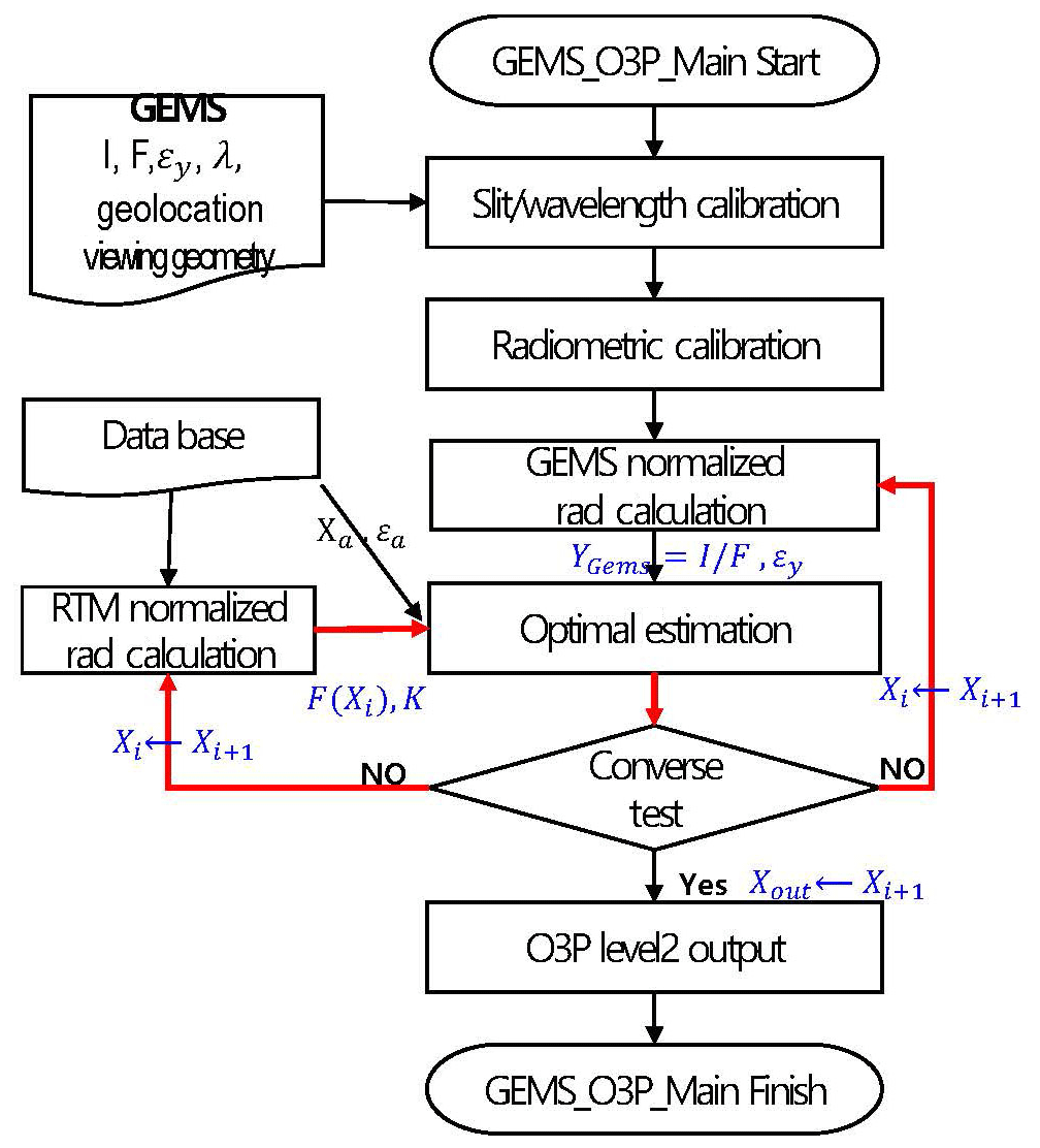
Figure 1 is a schematic diagram of the ozone profile algorithm. With the input of satellite measurements, the slit function is parameterized through cross-correlation between satellite irradiance and a high-resolution solar reference spectrum to be used for wavelength calibration and for high-resolution cross section convolution (Sun et al., 2017; Bak et al., 2019); a normalized Gaussian distribution is assumed to derive analytic slit functions for OMI. To remove the systematic errors between measured and calculated radiances, “soft calibration” is applied to measured radiances and then the logarithms of sun-normalized radiances are calculated as measurement vectors (Liu et al., 2010a; Cai et al., 2012; Bak et al., 2017). Measurement covariance matrices are constructed as diagonal matrices with components taken from the square of the measurement errors as measurement errors are assumed to be uncorrelated among wavelengths. In the OMI algorithm, a noise floor of 0.4 % (UV1) and 0.2 % (UV2) is used because OMI measurement errors underestimate other kinds of random noise errors caused by stray light, dark current, geophysical pseudo-random noise errors due to subpixel variability, motion when taking a measurement, forward model parameter error (random part), and other unknown errors into account (Huang et al., 2017). GEMS is expected to have similar retrieval sensitivity to tropospheric ozone and have at least comparable radiometric/wavelength accuracy (4 % including light source uncertainty/0.01 nm) to OMI. It is designed to provide hyperspectral radiances at a spectral resolution of 0.6 nm and spectral intervals of 0.2 nm, which are also similar to OMI (spectral resolution of 0.42–0.63 nm, sampling rate of 0.14–0.33 nm per pixel). A priori ozone information is taken from the tropopause-based (TB) ozone profile climatology which was developed for improving ozone profile retrievals in the upper troposphere and lower stratosphere (Bak et al., 2013b). The Vector LInearized Discrete Ordinate Radiative Transfer (VLIDORT) model (Spurr, 2006, 2008) is used to calculate normalized radiances and weighting function matrices for the atmosphere, with Rayleigh scattering and trace-gas absorption and with Lambertian reflection for both surface and cloud (Liu et al., 2010a). The ozone algorithm iteratively estimates the best ozone profiles within the retrieval converges (typically 2–3 iterations), together with other geophysical and calibration parameters (e.g., cloud fraction, albedo, BrO, wavelength shift, Ring parameter, mean fitting scaling parameter) for a better fitting accuracy even though some of the additional fitting parameters can reduce the degrees of freedom for signal of ozone. We should note here that GEMS data processing is expected to be different from OMI mainly in two ways: (1) OMI uses a depolarizer to scramble the polarization of light. However, GEMS has polarization sensitivity (required to be less than 2 %) and performs polarization correction using an RTM-based look-up table of atmospheric polarization state and pre-flight characterization of instrument polarization sensitivity in the level 0 to 1b data processing. The GEMS polarization correction is less accurate, and hence an additional fitting process might be required in the level 2 data processing, especially for ozone profiles that are more sensitive to the polarization error compared to other trace gases. (2) GEMS has a capability to perform diurnal observations and hence diurnal meteorological input data are required to account for the temperature-dependent Huggins band ozone absorption. Hence, the numerical weather prediction (NWP) model analysis data will be transferred to the GEMS Science Data Processing Center (SDPC).

Figure 1Flow chart of the GEMS ozone profile retrieval algorithm.

Download

2.2 Ozonesonde measurements

Ozonesondes are small, lightweight, and compact balloon-borne instruments capable of measuring profiles of ozone, pressure, temperature, and humidity from the surface to balloon burst, usually near 35 km (4 hPa); ozone measurements are typically reported in units of partial pressure (mPa) with vertical resolution of ∼100–150 m (WMO, 2014). Ozone soundings have been taken for more than 50 years, since the 1960s. The accuracy of ozonesonde measurements has been reported as 5 %–10 % with a precision of 3 %–5 %, depending on the sensor type, manufacturer, solution concentrations, and operational procedure (Smit et al., 2007; Thompson et al., 2007, 2017; Witte et al., 2017, 2018). Three types of instruments have been carried on balloons, i.e., the modified Brewer–Mast (MBM), the carbon–iodine cell (CI), and the electrochemical concentration cell (ECC). These are disposable instruments and hence launched weekly for long-term operation.

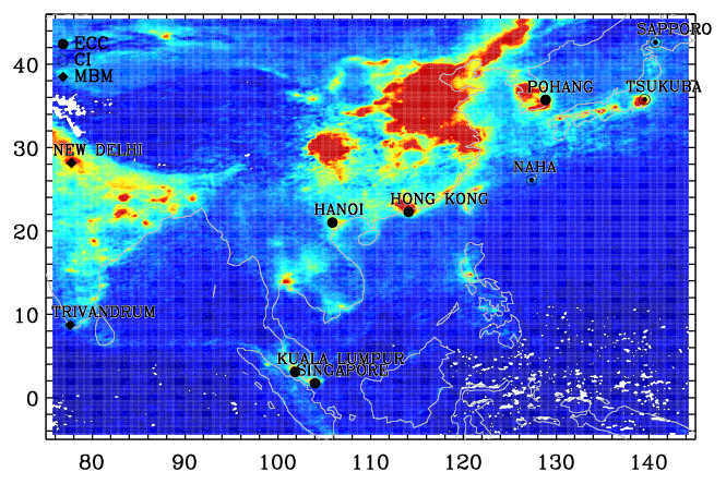
Figure 2Geographic locations of the ozonesonde stations available since 2005 over the GEMS observation domain. Each symbol represents a different type sensor: the modified Brewer–Mast (MBM), the carbon–iodine cell (CI), and the electrochemical concentration cell (ECC). The background map illustrates the OMI NO₂ monthly mean in June 2015.

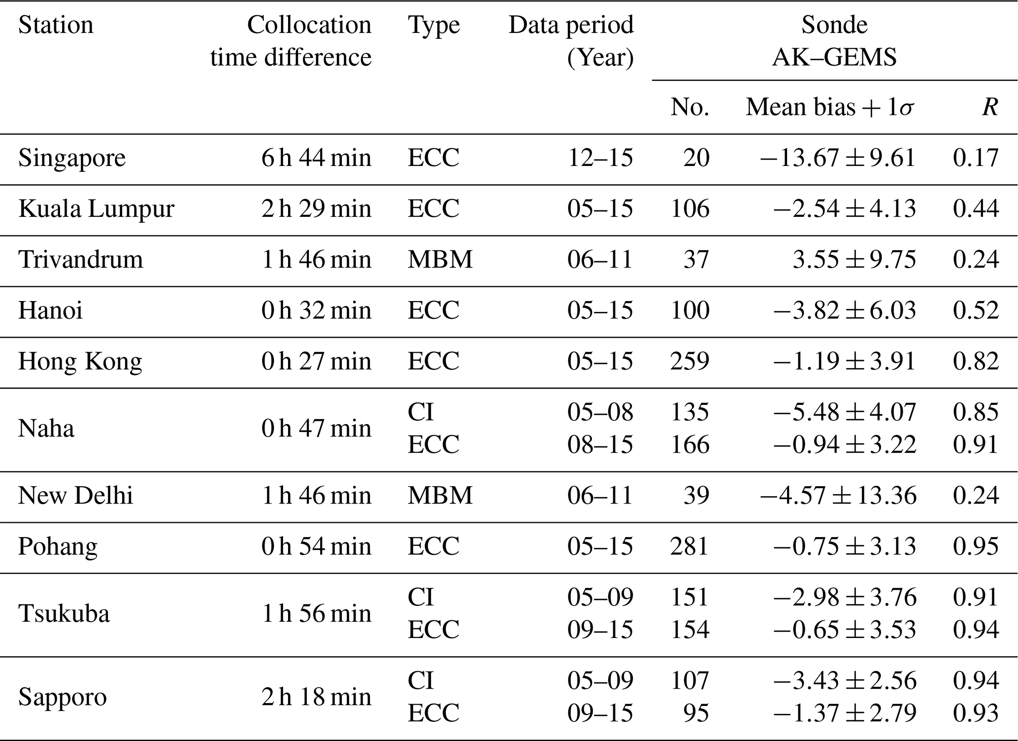
Figure 2 displays the locations of 10 ozonesonde sites focused on in this study within the GEMS domain bordering from 5^∘ S (Indonesia) to 45^∘ N (south of the Russian border) and from 75 to 145^∘ E. A summary of each ozonesonde site is presented in Table 1. Most of measurements are collected from the WOUDC network, except that Pohang soundings are provided from the Korea Meteorological Administration (KMA), and Kuala Lumpur and Hanoi measurements are from the Southern Hemisphere Additional OZonesondes (SHADOZ) network. In South Korea, ECC sondes have been launched every Wednesday since 1995 at Pohang, without significant time gaps. There are three Japanese stations (Naha, Tsukuba, and Sapporo) where the CI-type sensor was used before switching to the ECC-type sensor as of early 2009, and two Indian stations at New Delhi and Trivandrum using the modified BM (MBM) sensor. The rest of stations (Hanoi, Hong Kong, Kuala Lumpur and Singapore) use only ECC. Most stations employ ECC sensors, but inhomogeneities in ECC ozonesondes are strongly correlated to preparation and correction procedures. There are two ECC sensor manufacturers: the Science Pump Corporation (model type SPC-6A) and the Environmental Science Corporation (model type EN-SCI-Z/1Z/2Z). Since 2011 EN-SCI has been taken over by Droplet Measurement Technologies (DMT) Inc. The recommend mixtures of the standard sensing solution (SSI) are 1.0 % potassium iodide (KI)/full buffer (SST1.0) and 2.0 % KI/no buffer (SST0.5) for the SPC and EN-SCI sondes, respectively by the ASOPOS (Assessment for Standards on Operation Procedures for Ozone Sondes) (Smit et al., 2012). Among ECC stations, Pohang, Hong Kong, and the Japanese stations have applied the standard sensing solution to all ECC sensors manufactured by one company. In Singapore, the ozonesonde manufacture was changed in late 2015 from EN-SCI to SPC, while SST 0.5 was switched to SST1.0 as of 2018. Two SHADOZ stations (Kuala Lumpur and Hanoi) have applied the standard sensing solution just since 2015. Hanoi changed sensing solution four times with two different ozonesonde manufacturers; Kuala Lumpur operated only with SPC 6A-SST1.0 combination until 2014 but with four different radiosonde manufacturers. Therefore the SHADOZ datasets were homogenized (Witte et al., 2017) through the application of transfer functions between sensors and solution types. The post-processing could be applied by data users to some WOUDC datasets given a correction factor, which is the ratio of integrated ozonesonde column (appended with an estimated residual ozone column above burst altitude) and total ozone measurements from co-located ground-based and/or overpassing satellite instruments. The above-burst column ozone is estimated with a constant ozone mixing ratio (CMR) assumption above the burst altitude (Japanese sites; Morris et al., 2013) or satellite-derived stratospheric ozone climatology (Indian sites; Rohtash et al., 2016). No post-processing is done for Pohang, Hong Kong, and Singapore. Most stations made weekly or biweekly regular observations, except for Indian stations with irregular periods of 0–4 per month and for Singapore with monthly observations.

Table 1List of ozonesonde stations.

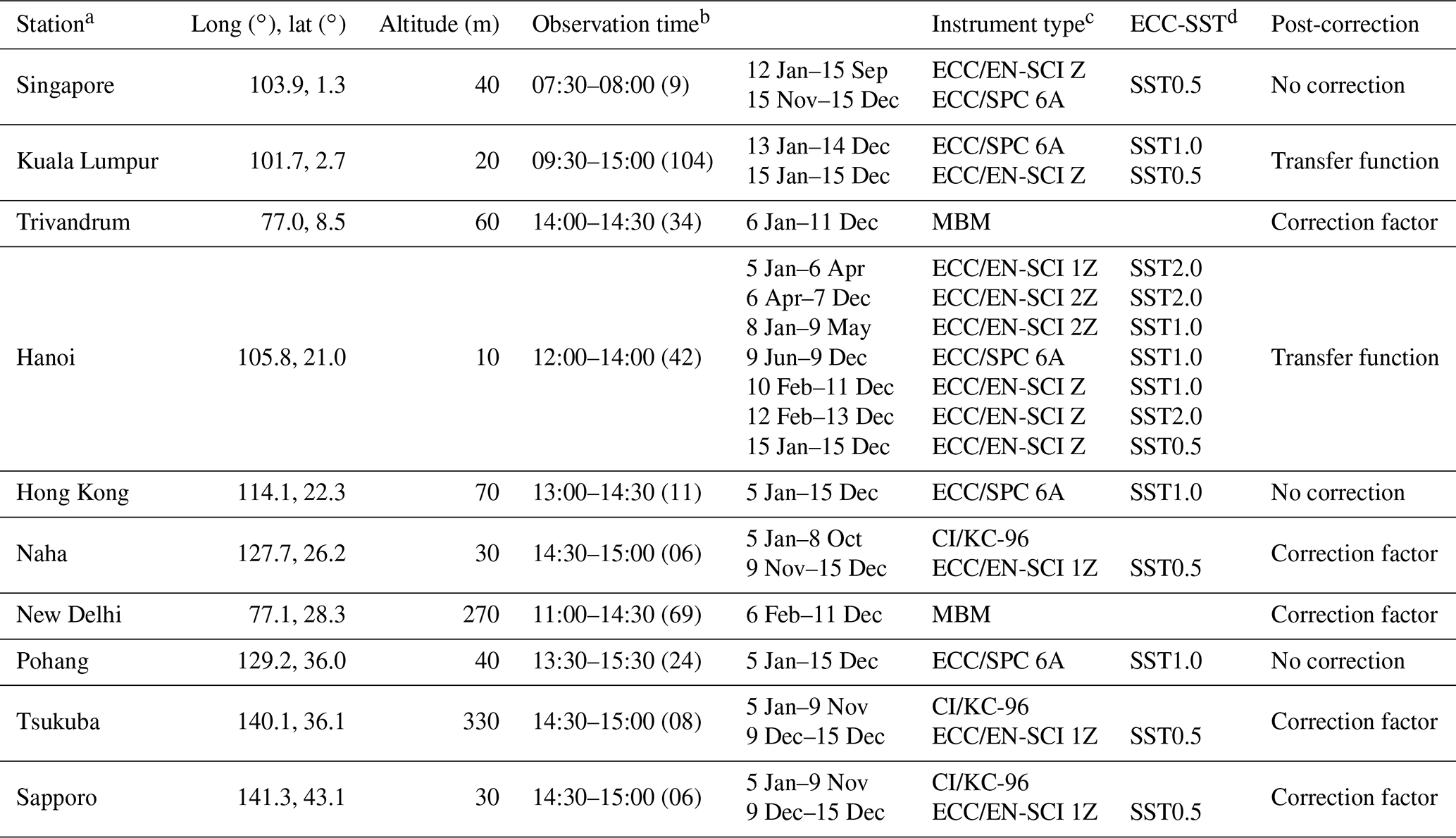
^a Data are downloaded from the WOUDC (http://woudc.org, last access: 7 July 2019) data archive, except for Kuala Lumpur and Hanoi, which are from the SHADOZ (https://tropo.gsfc.nasa.gov/shadoz/, last access: 7 July 2019) network, and Pohang, which are from the Korea Meteorological Administration (KMA). ^b The range of the observation time (LT) with 1σ standard deviations of them (min) in parentheses. ^c Ozonesonde sensor type (ECC indicates electrochemical condensation cell, CI the carbon–iodine cell Japanese sonde, and MBM the modified Brewer–Mast Indian sonde). ECC sensors manufactured by either ECC sensor manufacturers: Science Pump Corporation (model type SPC-6A) or Environmental Science cooperation (model type EN-SCI-Z/1Z/2Z). ^d Potassium iodide (KI) cathode sensing solution type (SST) implemented in ECC ozone sensors: SST0.5 (0.5 % KI, half buffer), SST1.0 (1.0 % KI, full buffer), and SST 2.0 (2.0 % KI, no buffer). Singapore station changed it to SST1.0 as of 2018.

Download Print Version | Download XLSX

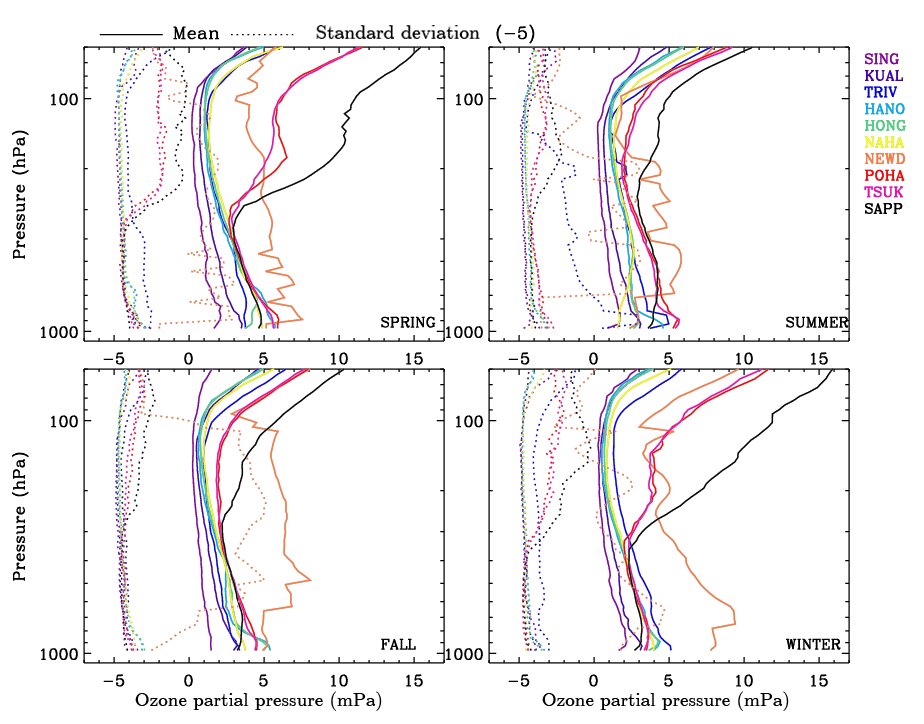
Figure 3Seasonal mean (solid) and standard deviation (dashed) profiles of ozonesonde soundings from 2005 to 2015 at the 10 sites listed in Table 1; 5 mPa is subtracted from standard deviations to fit the x axis.

Download

In Fig. 3 the seasonal means and standard deviations of ozonesonde measurements are presented to show the stability and characteristics of ozonesonde measurements at each site. Instabilities of measurements are observed from New Delhi ozonesondes. High surface ozone concentrations at Trivandrum in summer are believed to be caused by measurement errors because low levels of pollutants have been reported at this site under these geolocation and meteorological effects (Lal et al., 2000). Besides Trivandrum, Naha could be regarded as a background site according to low surface ozone (Fig. 3) and precursor concentrations (Fig. 2) compared to neighboring stations and previous studies (Oltmans et al., 2004; Liu et al., 2002). In the lower troposphere, high ozone concentrations are captured at Pohang, Tsukuba, and Sapporo in the summer due to enhanced photochemical production of ozone in daytime, whereas tropical sites Naha, Hanoi, and Hong Kong show ozone enhancements in spring, mainly due to biomass burning in Southeast Asia, with low ozone concentrations in summer due to the Asian monsoon and in winter due to tropical air intrusion (Liu et al., 2002; Ogino et al., 2013). Singapore and Kuala Lumpur are supposed to be severely polluted areas, but ozone pollution is not clearly captured over the seasons. This might be explained by the morning observation time at these two stations. In addition, instabilities of Singapore measurements are noticeable, including abnormally large variability and very low ozone concentration in the stratosphere. The effect of stratospheric intrusions on the ozone profile shape is dominant at mid-latitudes (Pohang, Tsukuba, and Sapporo) during the spring and winter when the ozonepause goes down to 300 hPa, with larger ozone variabilities in the lower stratosphere and upper troposphere, whereas the ozonepause is around 100 hPa with much less variability of ozone in other seasons.

2.3 Comparison methodology

The GEMS ozone profile algorithm is applied to OMI BUV measurements for 300–330 nm to simulate GEMS ozone profile retrievals at coincident locations listed in Table 1. The coincidence criteria between satellite and ozonesondes are ±1.0^∘ in both longitude and latitude and ±12 h in time, and then the closest pixel is selected. The Aura satellite carrying OMI crosses the Equator always at ∼ 13:45 local time (LT); thus OMI measurements are collocated within 3 h to ozonesonde soundings in the afternoon (13:00–15:00). Weekly based sonde measurements provide 48 ozone profiles at a maximum for a year. The number of collocations is on average 40 from 2004 October to 2008, but this reduced to ∼20 recently due to the screened OMI measurements affected by the “row anomaly” which was initially detected at two rows in 2007, and it has seriously spread to other rows since January 2009 (Schenkeveld et al., 2017). From July 2011 the row anomaly extends up to ∼50 % of all rows. Correspondingly, the average collocation distance increases from 57.5 to 66.6 km before and after the occurrence of the row anomaly. The impact of spatiotemporal variability on the comparison will be much reduced for GEMS due to its higher spatiotemporal resolution (7 km × 8 km at Seoul, hourly) against OMI (48 km × 13 km at nadir in UV1, daily).

To increase the validation accuracy, data screening is implemented for both ozonesonde observations and satellite retrievals according to Huang et al. (2017). For ozonesonde observations, we screen ozonesondes with balloon-bursting pressures exceeding 200 hPa, gaps greater than 3 km, abnormally high concentration in the troposphere (> 80 DU), and low concentration in the stratosphere (< 100 DU). Among WOUDC sites, the Japanese and Indian datasets include a correction factor which is derived to make better agreement between integrated ozonesonde columns and correlated reference total ozone measurements as mentioned in Sect. 2.2. In Fig. 4, Japanese ozonesondes are compared against GEMS simulations when a correction factor is applied or not to each CI and ECC measurement, respectively. Morris et al. (2013) recommended restricting the application of this correction factor to the stratospheric portion of the CI ozonesonde profiles due to errors in the above-burst column ozone. Our comparison results illustrate that applying the correction factor reduces the vertical fluctuation of mean biases in ozone profile differences with insignificant impact on their standard deviations. Therefore we decide to apply this correction factor to the sonde profiles if this factor ranges from 0.85 to 1.15. Because of a lack of retrieval sensitivity to ozone below clouds and lower tropospheric ozone under extreme viewing conditions, GEMS simulations are limited to cloud fraction less than 0.5, solar zenith angles (SZAs) less than 60^∘, and fitting rms (i.e., root mean square of fitting residuals relative to measurement errors) less than 3.

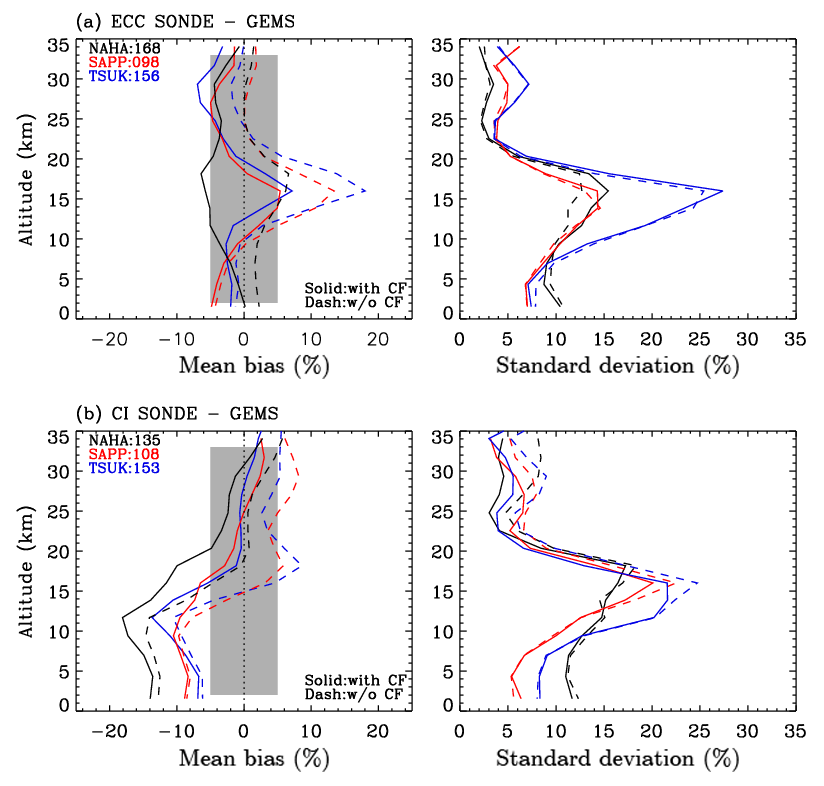
Figure 4Effects of applying a correction factor (CF) to (a) ECC and (b) CI ozonesonde measurements, respectively, on comparisons with simulated GEMS ozone profile retrievals. Solid and dashed lines represent the comparisons with and without applying a CF, respectively, at each Japanese station. The number of data point is included in the legends.

Download

Due to the different units of ozone amount between satellites and ozonesondes, we convert ozonesonde-measured partial pressure ozone values (mPa) to partial column ozone (DU) at the 24 retrieval grids of the satellite for the altitude range from surface to the balloon-bursting altitudes. Ozonesonde measurements are obtained at a rate of a few seconds and then typically averaged into altitude increments of 100 m, whereas retrieved ozone profiles from nadir BUV satellite measurements have much coarser vertical resolution of 10–14 km in the troposphere and 7–11 km in the stratosphere, based on OMI retrievals. Consequently, satellite observations capture only the smoothed structures of ozonesonde soundings, especially near the tropopause, where a sharp vertical transition of ozone within 1 km is observed, and in the boundary layer due to the insufficient penetration of photons. Satellite retrievals unavoidably have an error compound due to its limited vertical resolution, called “smoothing error” in OE-based retrievals (Rodgers, 2000). It could be useful to eliminate the effect of smoothing errors on differences between satellites and sondes to better characterize other error sources in comparisons (Liu et al., 2010a). For this reason, satellite data have been compared to ozonesonde measurements smoothed to the satellite vertical resolution, together with original sonde soundings (Liu et al., 2010b; Bak et al., 2013b; Huang et al., 2017). The smoothing approach is

where x_sonde is the high-resolution ozonesonde profile, ${\widehat{x}}_{\mathrm{sonde}}$ the convolved ozonesonde profile into satellite vertical resolution, A the satellite averaging kernel, and x_a the a priori ozone profile.

In order to define tropospheric columns, both satellite retrievals and ozonesonde measurements are vertically integrated from the surface to the tropopause taken from daily National Centers for Environmental Prediction (NCEP) final (FNL) Operational Global analysis data (http://rda.ucar.edu/datasets/ds083.2/, last access: 7 July 2019). To account for the effect of surface height differences on comparison, ozone amounts from satellite data below the surface heights of ozonesondes are added to tropospheric columns of ozonesonde measurements and vice versa.

Table 2Comparison statistics (mean bias in DU, 1σ standard deviation in DU, and R, correlation coefficient) between GEMS-simulated tropospheric ozone column and ozonesonde measurements convolved with GEMS averaging kernels.

Download Print Version | Download XLSX

3.1 Comparison at individual stations

Witte et al. (2018) recently compared seven SHADOZ station ozonesonde records, including Hanoi and Kuala Lumpur in the GEMS domain, with total ozone and stratospheric ozone profiles measured by spaceborne nadir and limb-viewing instruments, respectively. In this comparison, the Hanoi station shows comparable or better agreement with the satellite datasets when compared to other sites. Morris et al. (2013) and Rohtash et al. (2016) thoroughly evaluated ozonesonde datasets over Japanese and Indian sites, respectively, but they did not address their measurement accuracy with respect to those at other stations. Validation of GOME TOC by Liu et al. (2006) showed relatively larger biases at Japanese CI stations, and validation of OMI TOC by Huang et al. (2017) showed both larger biases and standard deviations at the Indian MBM sites. In South Korea, regular ozonesonde measurements are taken only from Pohang, but these measurements have been insufficiently evaluated; only the stratospheric parts of these measurements were quantitatively assessed against satellite solar occultation measurements by Halogen Occultation Experiment (HALOE) from 1995 to 2004 in Hwang et al. (2007), but only 26 pairs were compared despite the coarse coincident criteria (48 h in time, ±4.5^∘ in latitude, ±9^∘ in longitude). Therefore, it is important to perform quality assessment of ozonesonde measurements to identify a reliable reference dataset for GEMS ozone profile validation.

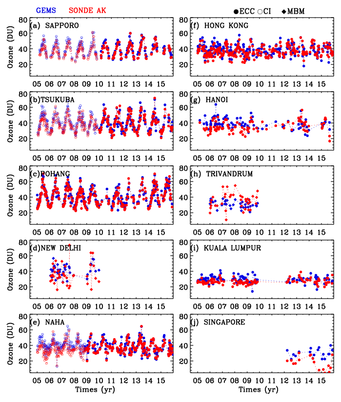
Figure 5Time series of tropospheric ozone columns (DU) of GEMS-simulated ozone profile retrievals (blue) and ozonesonde measurements convolved with GEMS averaging kernels (red) from 2005 to 2015 at 10 stations listed in Table 1.

Download

For this purpose, we illustrate tropospheric ozone columns (TOCs) as a function of time for individual stations listed in Table 1, measured with three different types of ozonesonde instruments and retrieved with GEMS simulations (Fig. 5), respectively. The goal of this comparison is to identify any abnormal deviation of ozonesonde measurements relative to satellite retrievals, so we exclude the impact of the different vertical resolutions between instruments and satellite retrievals in this comparison by convolving ozonesonde data with satellite averaging kernels. At midlatitude sites (Pohang, Sapporo, and Tsukuba) both ozonesonde and simulated retrievals show the distinct seasonal TOC variations with values ranging from ∼35 to ∼40 DU. Extratropical sites (Naha, Hong Kong, and Hanoi) show less seasonal variations, 30 to 50 DU, whereas fairly constant concentrations are observed at Kuala Lumpur and Singapore in the tropics. Both ozonesonde observations and simulated retrievals illustrate similar seasonal variabilities at these locations. At New Delhi and Trivandrum, on the other hand, MBM ozonesonde measurements abnormally deviate from 10 to 50 DU compared to the corresponding satellite retrievals and ozonesonde measurements at stations at similar latitudes.

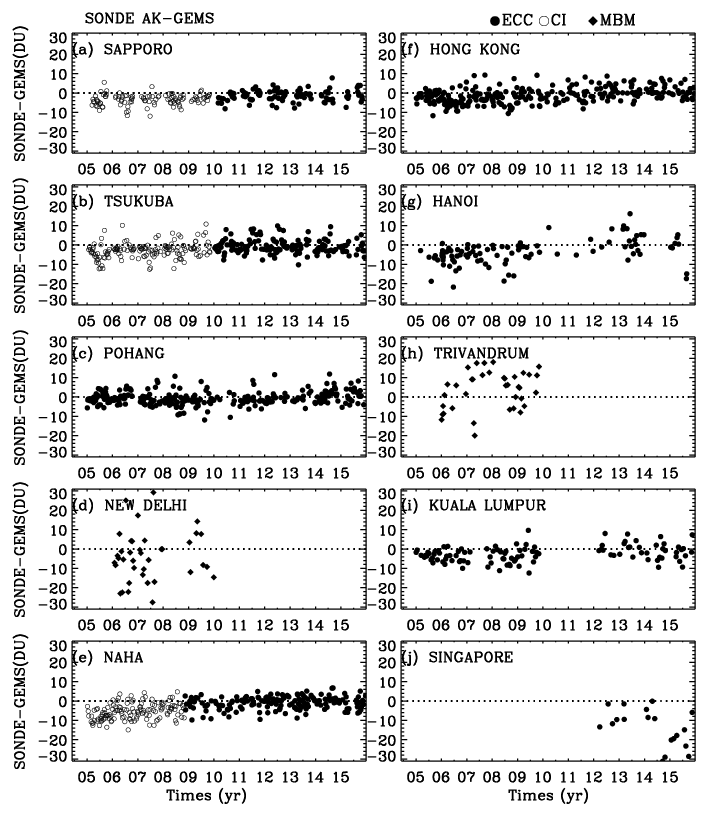
Figure 6Same as Fig. 5 but for absolute differences of tropospheric ozone columns (DU) between ozonesonde measurements and GEMS-simulated retrievals.

Download

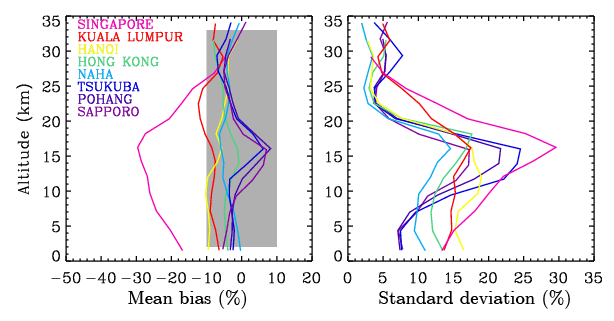
Figure 7Mean biases and 1σ standard deviations of the differences between ozonesonde convolved with GEMS averaging kernels and GEMS-simulated ozone retrievals as a function of GEMS layers, at individual ECC ozonesonde stations. The relative difference is defined as (Sonde AK–GEMS) × 100 %/(a priori), where AK indicates averaging kernel.

Download

In Fig. 6 time-dependent errors in differences of TOC between ozonesonde and simulated GEMS retrievals are evaluated with the corresponding comparison statistics in Table 2. Simulated retrievals show a strong correlation of ∼0.8 or much larger with ozonesonde measurements at Pohang, Hong Kong, and three stations from Japan, and with a low correlation of ∼0.5 at other SHADOZ stations in the tropics. However, Indian stations show poor correlation of 0.24. Mean biases and standard deviations are much smaller at stations where a strong correlation is observed; they are $\sim \mathrm{1}\pm \sim \mathrm{4}$ DU at most ECC stations but deviated to $\sim \mathrm{4}\pm \sim \mathrm{10}$ DU at MBM stations. In conclusion, we should exclude ozonesonde observations measured by MBM to remove irregularities in a reference dataset for validating both GEMS-simulated retrievals in this study and GEMS actual retrievals in future studies. Moreover, time series of ozonesonde and simulated retrievals show a significant transition at three Japanese stations as of late 2008 and early 2009, when the ozonesonde instruments were switched from CI to ECC. This transition could be affected by spaceborne instrument degradation, but the impact of balloon-borne instrument change on them is predominant based on a less time-dependent degradation pattern at neighboring stations during this period. CI ozonesondes noticeably underestimate atmospheric ozone by 2–3 DU compared to ECC, and thereby GEMS TOC biases relative to CI measurements are estimated as −2 to −5 DU, but these biases are reduced to < 1.5 DU when compared with ECC. Therefore, we decide to exclude these CI ozonesonde observations for evaluating GEMS-simulated retrievals. Compared to other ECC stations, Hanoi station often changed sensing solution concentrations and pH buffers (Table 1), which might cause the irregularities due to remaining errors even though transfer functions were applied to ozonesonde measurements to account for errors due to the different sensing solution (Witte et al., 2017). This fact might affect the relatively worse performance compared to a neighboring station, Hong Kong, where the 1.0 % KI buffered sensing solution (SST1.0) to ECC/SPC sensors has been consistently applied.

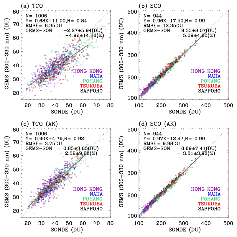
Figure 8(a, b) Scatter plots of GEMS vs. ozonesonde for tropospheric and stratospheric ozone columns, respectively. Panels (c) and (d) are the same as the upper ones, except that ozonesonde measurements are convolved with GEMS averaging kernels. A linear fit between them is shown in solid lines, with the 1:1 lines (dotted lines). The legends show the number of data points (N), the slope and intercept of a linear regression, and correlation coefficient (r), with mean biases and 1σ standard deviations for absolute (DU) and relative differences (%), respectively. Note that we use 5 stations identified as a good reference among 10 stations listed in Table 1 in this comparison.

Download

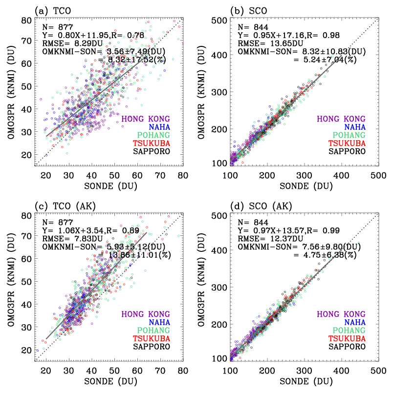
Figure 9Same as Fig. 8 but for validating OMI standard ozone profiles (OMO3PR) produced by the KNMI OE-based algorithm.

Download

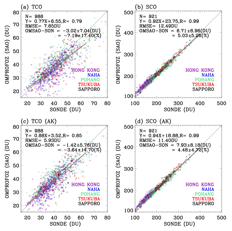
Figure 10Same as Fig. 8 but for validating OMI research ozone profiles (OMPROFOZ) produced by the SAO OE-based algorithm.

Download

Figure 7 compares differences of ozone profiles between ECC ozonesondes and GEMS-simulated retrievals at each station. Among ECC ozonesondes, Singapore's are in the worst agreement with GEMS simulations in both terms of mean biases and standard deviations, which could be explained by the discrepancy in collocation time. Sonde observations at Japan, Pohang, Hong Kong, and Hanoi stations, where balloons were launched in the afternoon (∼ 12:00–15:00 LT), are collocated within ∼1–2 h of OMI, whereas the time discrepancy increases to 7 h at Singapore, where ozonesondes are launched in the early morning. Photochemical ozone concentrations are typically denser in the afternoon than in the morning, and hence ozonesonde measurements at Singapore are negatively biased relative to afternoon satellite measurements. For the reason mentioned above, the discrepancy in the observation time could also affect this comparison at Kuala Lumpur, where sondes were mostly launched in the late morning, 2–3 h prior to the OMI passing time, and thereby ozonesonde measurements tend to be negatively biased. These indicate that diurnal variations of tropospheric ozone are visible in ozonesonde measurements, emphasizing the utility of hourly geostationary ozone measurements. The comparison results could be characterized with latitudes. In the midlatitudes (Pohang, Tsukuba, and Sapporo), noticeable disagreements are commonly seen in the tropopause region where mean biases/standard deviations are ∼10 %/∼15 % larger than those in the lower troposphere. In the extratropics (Hong Kong, Naha), consistent differences of a few percent are seen over the entire altitude range with standard deviations of 15 % or less below the tropopause (∼15 km). Hanoi and Kuala Lumpur show significantly larger biases/standard deviations compared to other ECC stations. At Hanoi inconsistencies of solution concentrations and pH buffers might influence this instability. At Kuala Lumpur the inconsistencies of observation times might be one of the reasons, considering its standard deviations of ∼100 min but mostly less than 30 min at other stations. Therefore, we screen out Singapore, Kuala Lumpur, and Hanoi, together with all MBM measurements at Indian stations and CI measurements at Japanese stations to improve the validation accuracy of GEMS-simulated retrievals in next section. Thus, stations where the standard procedures for preparing and operating ECC sondes are consistently maintained are adopted as an optimal reference for this work.

3.2 Evaluation of GEMS-simulated ozone profile retrievals

The GEMS-simulated retrievals are assessed against ECC ozonesonde soundings at five stations (Hong Kong, Pohang, Tsukuba, Sapporo, and Naha) identified as a good reference in the previous section. The comparison statistics include mean bias and standard deviation in the absolute/relative differences, correlation coefficients, linear regression results (slope (a), intercept (b), error); the error of the linear regression is defined as $\frac{\mathrm{1}}{n}\sqrt{\sum _i^n{\left(y_{\mathrm{GEMS}}-y_{\mathrm{fit}}\right)}^{\mathrm{2}}}$, where $y_{\mathrm{fit}}=a\cdot y_{\mathrm{sonde}}+b$. In Fig. 8, GEMS-simulated retrievals are plotted as functions of ozonesondes with and without the vertical resolution smoothing, respectively, for the stratospheric and tropospheric columns. GEMS simulations underestimate the tropospheric ozone by $\sim \mathrm{2.27}\pm \mathrm{5.94}$ DU and overestimate the stratospheric ozone by $\sim \mathrm{9.35}\pm \mathrm{8.07}$ DU relative to high-resolution ozonesonde observations. This comparison demonstrates good correlation coefficients of 0.84 and 0.99 for troposphere and stratosphere, respectively. This agreement is degraded if the rejected ECC sondes (Kuala Lumpur, Hanoi, and Singapore) are included; for example, the slope decreases from 0.68 to 0.64 while the RMSE increases 6.35 and 6.76 DU for TOC comparison. Smoothing ozonesonde soundings to GEMS vertical resolution improves the comparison results, especially for the tropospheric ozone columns; standard deviations are reduced by ∼5 % with mean biases of less than 1 DU. Similar assessments are performed for OMI standard ozone profiles based on the KNMI OE algorithm (Kroon et al., 2011) hereafter referred to as OMO3PR (KNMI) in Fig. 9 and the research product based on the SAO algorithm (Liu et al., 2010) hereafter referred to as OMPROFOZ (SAO) in Fig. 10, respectively. It implies that GEMS gives good information on stratospheric ozone columns (SOCs) comparable to both the OMI KNMI and SAO products in spite of insufficient information on Hartley ozone absorption in GEMS. Furthermore, a better agreement of GEMS TOCs with ozonesonde is found than with the others due to different implementation details. As mentioned in Sect. 2.1., the GEMS algorithm is developed based on the heritages of the SAO ozone profile algorithm with several modifications. The two main modifications are as follows: (1) a priori ozone climatology was replaced with a tropopause-based ozone profile climatology to better represent the ozone variability in the tropopause, and (2) irradiance spectra used to normalize radiance spectra and characterize instrument line shapes are prepared by taking a 31 d moving average instead of a climatological average to take into account for the time-dependent instrument degradation. These modifications reduce somewhat the spread in deviations of satellite retrievals from sondes, especially in TOC comparison. KNMI retrievals systematically overestimate the tropospheric ozone by ∼6 DU (Fig. 10c), which corresponds to the positive biases of 2 %–4 % in the integrated total columns of KNMI profiles relative to Brewer observations (Bak et al., 2015). As mentioned in Bak et al. (2015), the systematic biases in ozone retrievals are less visible in SAO-based retrievals (simulated GEMS data, OMPROFOZ), as systematic components of measured spectra are taken into account for using an empirical correction called “soft calibration”.