the Creative Commons Attribution 4.0 License.
the Creative Commons Attribution 4.0 License.
 | 08 Oct 2019
Validation of OCO-2 error analysis using simulated retrievals
Susan S. Kulawik
Chris O'Dell
Robert R. Nelson
Thomas E. Taylor
Characterization of errors and sensitivity in remotely sensed observations of greenhouse gases is necessary for their use in estimating regional-scale fluxes. We analyze 15 orbits of the simulated Orbiting Carbon Observatory-2 (OCO-2) with the Atmospheric Carbon Observations from Space (ACOS) retrieval, which utilizes an optimal estimation approach, to compare predicted versus actual errors in the retrieved CO2 state. We find that the nonlinearity in the retrieval system results in XCO2 errors of ∼0.9 ppm. The predicted measurement error (resulting from radiance measurement error), about 0.2 ppm, is accurate, and an upper bound on the smoothing error (resulting from imperfect sensitivity) is not more than 0.3 ppm greater than predicted. However, the predicted XCO2 interferent error (resulting from jointly retrieved parameters) is a factor of 4 larger than predicted. This results from some interferent parameter errors that are larger than predicted, as well as some interferent parameter errors that are more strongly correlated with XCO2 error than predicted by linear error estimation. Variations in the magnitude of CO2 Jacobians at different retrieved states, which vary similarly for the upper and lower partial columns, could explain the higher interferent errors. A related finding is that the error correlation within the CO2 profiles is less negative than predicted and that reducing the magnitude of the negative correlation between the upper and lower partial columns from −0.9 to −0.5 results in agreement between the predicted and actual XCO2 error. We additionally study how the postprocessing bias correction affects errors. The bias-corrected results found in the operational OCO-2 Lite product consist of linear modification of XCO2 based on specific retrieved values, such as the CO2 grad del (), (“grad del” is a measure of the change in the profile shape versus the prior) and dP (the retrieved surface pressure minus the prior). We find similar linear relationships between XCO2 error and dP or but see a very complex pattern of errors throughout the entire state vector. Possibilities for mitigating biases are proposed, though additional study is needed.


The Orbiting Carbon Observatory-2 (OCO-2) was launched in July 2014 and began providing science data in September 2014, with the goal of estimating CO2 with the “precision, resolution, and coverage needed to characterize sources and sinks of this important green-house gas.” (Crisp et al., 2004). Validation of the ACOS/OCO-2 build 7 (referred to hereafter as v7) dataset (Eldering et al., 2017) versus measurements from the Total Carbon Column Network (TCCON) (Wunch et al., 2011) shows regional biases of about 0.5 ppm and standard deviations of 1.5 ppm (Wunch et al., 2017), though these errors are not entirely due to OCO-2 (TCCON and colocation errors also contribute). Biases are particularly concerning due to propagation of CO2 biases into flux biases (Basu et al., 2013; Chevallier et al., 2014; Feng et al., 2016). OCO-2 error analysis uses Rodgers (2000), which gives a statistical estimate of errors using first-order analysis that assumes that the forward model is linear and estimates errors due to smoothing, radiance measurement error, and interferent species. The predicted XCO2 errors for v7 OCO-2 are typically 0.4 ppm for ocean glint and 0.5 ppm for nadir land, which underestimate the actual errors by at least a factor of 2 (Wunch et al., 2017). The cause of regional biases is thought to be underestimated interferent error or missing components of error analysis but is not well understood. Connor et al. (2016) found that missing physics in the forward model (e.g., more aerosol types, spectroscopy error, instrument error) leads to significantly larger posterior uncertainties than predicted by the current Atmospheric Carbon Observations from Space (ACOS) error analysis, using a purely linear error estimation framework. However, this study finds that nonlinear retrievals using this relatively simple simulation system (e.g., no spectroscopic errors, no instrument noise, consistent aerosol types between the true and retrieved states) also show a similar relationship between predicted and actual errors, with the actual error about twice the predicted one.
Cressie et al. (2016) estimates the size of second-order terms of the error analysis. The second-order terms contain derivatives of the averaging kernel, gain matrix, and Jacobians with respect to state parameters. Cressie et al. (2016) estimates that the errors resulting from second-order error analysis are on the order of 0.2 ppm, but this analysis was dependent on the states and sizes of deviations used to calculate the second-order derivatives. Cressie et al. (2016) found that second-order terms can cause both larger errors and biased results.
This paper explores the errors in the full physics retrieval system using a simulated system with no mismatches in the retrieval versus true state vector and no spectroscopy or instrument errors. The actual error covariance of (retrieved minus true) for this retrieval system is about twice the predicted errors. The linear analysis of Connor et al. (2016) does not explain the higher errors in this work, because the simulations in this work do not include unaccounted errors sources. Cressie et al. (2016) also does not explain the higher actual errors, because Cressie et al. (2016) estimates the second-order error as about 0.2 ppm, whereas the unaccounted error is about 0.8 ppm in this paper. In order to identify the source of the unaccounted error, actual errors are compared to the predicted linear errors for a series of setups.
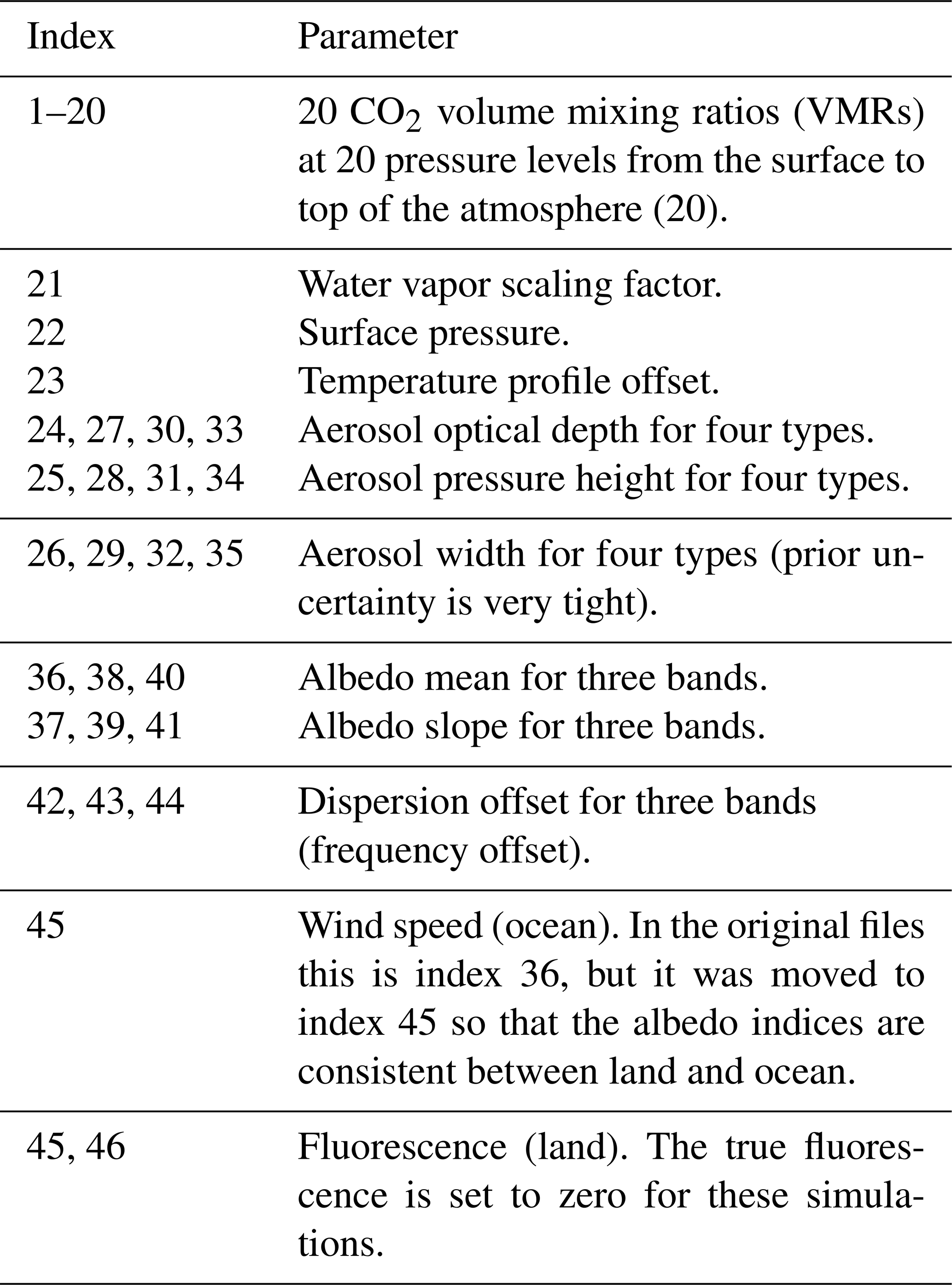
The ACOS Level 2 (L2) full physics retrieval algorithm used to estimate XCO2 from OCO-2 employs optimal estimation using three near-infrared bands: (1) 0.76 µm containing significant O2 absorption (O2 A band), (2) around 1.6 µm containing weak CO2 absorption (weak CO2 band), and (3) near 2.1 µm containing strong CO2 absorption (strong CO2 band). Prior to the main retrieval, a series of fast preprocessing steps are performed for quality analysis (primarily to screen out clouds) and to provide estimates of chlorophyll fluorescence (Frankenberg et al., 2016). Only soundings that are deemed sufficiently clear are selected to be processed by the computationally expensive L2 retrieval. In the optimal estimation L2 retrieval used in this simulation, 45–46 retrieval parameters are simultaneously estimated, including CO2 volume mixing ratios (VMRs) at 20 pressures, albedos in three bands, four types of aerosols, meteorological parameters (temperature, water vapor, surface pressure), dispersion (frequency offset), wind speed (ocean only), and fluorescence (land only).
The retrieved CO2 profile is then collapsed into a column, XCO2. Recent work has alternatively partitioned the information into two partial columns (Kulawik et al., 2017). Postprocessing quality screening and linear bias corrections based on various L2 retrieved parameters are then performed on XCO2. The corrections are based on the slope of XCO2 error versus different retrieved values, where the XCO2 error is estimated from retrieved XCO2 minus either (a) a constant value in the Southern Hemisphere, the Southern Hemisphere approximation; (b) values from surface-based observations from TCCON stations; (c) the mean of small areas (less than 1∘); or (d) a multimodel mean (Mandrake et al., 2017). We study the effects of the postprocess bias correction in Sect. 4.3. The simulations in this paper differ from the operational retrieval in that the fluorescence true state is set to zero, although fluorescence is still retrieved; and amplitudes of spectral residual patterns are not retrieved; except for these minor differences, these simulated retrievals are identical to the operational v7 retrievals. We refer the interested reader to O'Dell et al. (2018) for a full description of the operational retrieval, including retrieved variables and bias correction.
Simulation studies can be used to understand and probe retrieval results. There are many different ways to assess errors, listed here in order of increasing complexity and nonlinearity.
-
Linear estimates of errors, which assume moderate linearity of the retrieval system (Connor et al., 2008, 2016), useful for surveying impacts of different errors with linear assumptions.
-
Error estimates from nonlinear retrievals of simulated radiances using a fast, simplified radiative transfer, called the “surrogate model” (Hobbs et al., 2017). This system does not result in the discrepancy of larger actual versus predicted error.
-
Error estimates from nonlinear retrievals of simulated radiances generated using the operational L2 forward model, called the “simplified true state”, which has the advantage that the true state is within the span of the retrieval vector and the linear estimate should be valid.
-
Error estimates from nonlinear retrievals of simulated radiances using a more complex and accurate radiative transfer model to generate the observed radiances (e.g., Raman scattering, polarization handling, surface albedo changes effects) and discrepancies between the true and retrieved state vectors (e.g., aerosol type mismatches between the true and retrieval state vector, albedo shape variations) (e.g., O'Dell et al., 2012).
This paper uses system (3), which makes it easier to interpret the actual versus expected performance of the retrieval system. System (3) was used because preliminary studies seemed to find that the performance of systems (3) and (4) was comparable (results not shown). Note that the observed radiance is generated with slightly different code than the retrieval system, but they are matched as closely as possible.
2.1 Description of the OCO-2 L2 retrieval algorithm and error diagnostics
The ACOS optimal estimation approach is described in O'Dell et al. (2012, 2018) and Crisp et al. (2012). In this section we review the parameters in the retrieval vector and the equations for error estimates. The retrieved parameters for this simulation study are shown in Table 1.
All non-CO2 parameters are called “interferents”, and the propagation of errors from these parameters into CO2 is called “interferent error”.
The a priori covariance matrix for CO2 has the dimensions 20×20 and has strong correlations as shown in Fig. 2 of O'Dell et al. (2012). The CO2 a priori error is 48 ppm at the surface, 12 ppm in the midtroposphere, and 1.4 ppm in the stratosphere. The larger variability near the surface allows more variability in the retrieved CO2 profile near the surface. However, in the ACOS retrieval, about 8 % of the true midtropospheric CO2 variations are incorrectly attributed to surface variations based on the bias correction of (Kulawik et al., 2017). The a priori errors for other parameters are all uncorrelated in the a priori covariance and can be found in the L2 product file.
The predicted errors, found in the OCO-2 L2 product as “XCO2_error_components”, are based on the assumption that the nonlinear, iterative retrievals can be represented as a linear estimate (Connor et al., 2008; Rodgers, 2000), and shown in Eq. (1).
where
-
is the retrieved CO2 profile, size nCO2 (20 for OCO-2) – this variable is called “u” in Connor et al. (2008), called “v” here so as not to be confused with a different U variable introduced later;
-
va is the a priori CO2 profile, size nCO2;
-
vtrue is the true CO2 profile, size nCO2;
-
Avv is the nCO2×nCO2 CO2 profile averaging kernel;
-
Ave(etrue−ea) is the cross-state error representing the propagation of error from non-CO2 retrieved parameters, e (aerosols, albedo, etc.), into retrieved CO2;
-
ea is the a priori interferent value, size ninterf – for this work, ninterf is 26 (27) for ocean (land);
-
etrue is the true interferent value, size ninterf;
-
Ave is size nCO2×ninterf;
-
Gv is the gain matrix for CO2, size nCO2×nf, where nf is the number of spectral points; and
-
ε is the spectral error, also called “measurement error”, size nf.
The full gain matrix, G, maps from spectral signals to retrieval parameter changes and is
where K is the Jacobian (or Kernel) matrix, and Sε is the error covariance of the spectral error, ε. Note that G is size n×nf, where is the total number of retrieved parameters. K is a matrix of derivatives giving the sensitivity of the radiance at each frequency to each retrieved parameter; e.g., for the CO2 parameter at 800 hPa,
An assumption of the ACOS retrieval system is that the Jacobians are fairly invariant during the retrieval process, as is the assumption for nearly all optimal estimation retrievals (see, e.g., Rodgers, 2000).
The averaging kernel, A, is one of the most fundamental and useful quantities in Bayesian inversion theory. It describes the predicted linear dependence of the retrieved state on the true state and prior. The diagonal of the averaging kernel gives the degrees of freedom for signal for each retrieval parameter. The averaging kernel is calculated as
As will be shown in Sect. 3.1, we find that varies depending on the retrieved state (indicating nonlinearity), which would result in an error in retrieved CO2 that is not captured in the predicted errors.
The linear estimate describes the response of the retrieval system to instrument errors and incorrect a priori inputs, based on the strengths of the Jacobians (representing sensitivity of the radiances to the retrieval state) and constraints (how much pressure is applied to parameters to stay near the a priori inputs). The linear estimate in Eq. (1) is used to estimate the errors, and for simulations, where we know all the inputs, it is useful to test each component of Eq. (1).
After an inversion is complete, the pressure weighting function h (size nCO2) is used to convert the retrieved CO2 profile to XCO2 by tracking the contribution from each level to the column quantity:
The predicted errors on the estimated XCO2 arise from three separate terms in Eq. (1):
-
Gxε results from the errors on the measured radiances (measurement error),
-
Avv(vtrue−va) results from both imperfect sensitivity and constraint choices (smoothing error), and
-
Ave(vtrue−va) results from jointly retrieved species propagated into CO2 (interferent error).
The CO2 profile can also be partitioned into a lower and upper partial column (Kulawik et al., 2017). These can be calculated using equations similar to Eq. (5), with h set for the lower partial column air mass (LMT) by zeroing out the upper 15 levels, and h set for the upper partial column (U) by zeroing out the lower 5 levels. In this work, the lower and upper partial columns are explored to try to understand the reasons behind the underpredicted XCO2 errors and the effect of the component of the bias correction.
One useful diagnostic is an estimate of how well the modeled radiances match the observed radiances for each of the three OCO-2 spectral bands:
where rfit is the fit radiance, robs is the observed radiance, and ε is the radiance error.
In reality, Eq. (1) would contain many additional error terms that are not considered in these simulations, e.g., spectroscopy, instrument characteristics, aerosol mismatch errors (i.e., picking the wrong aerosol type to retrieve). These are discussed in detail in Connor et al. (2016) as linear error estimates. The results reported here only address errors in the full nonlinear retrieval system for the actual retrieved variables; they do not include errors from unincluded physics or other error sources (such as spectroscopy error). In the analysis presented in Sect. 3, each of the diagnostics given in Eqs. (1) through (5) will be used to examine the error estimates on the simulations and compared to previously published results on real OCO-2 data.
2.2 Description of the simulated dataset
The simulated dataset analyzed in this study is comprised of a set of realistic retrievals using the ACOS b3.4 version of the retrieval algorithm. It is a slightly modified version of that described in detail in O'Dell et al. (2012) (which discussed b2.9) and described more fully in O'Dell et al. (2018). Table 2 shows the most important changes to the L2 retrieval algorithm between b2.9 and b3.4.
Table 2Updates in the simulated retrieval system since O'Dell et al. (2012).
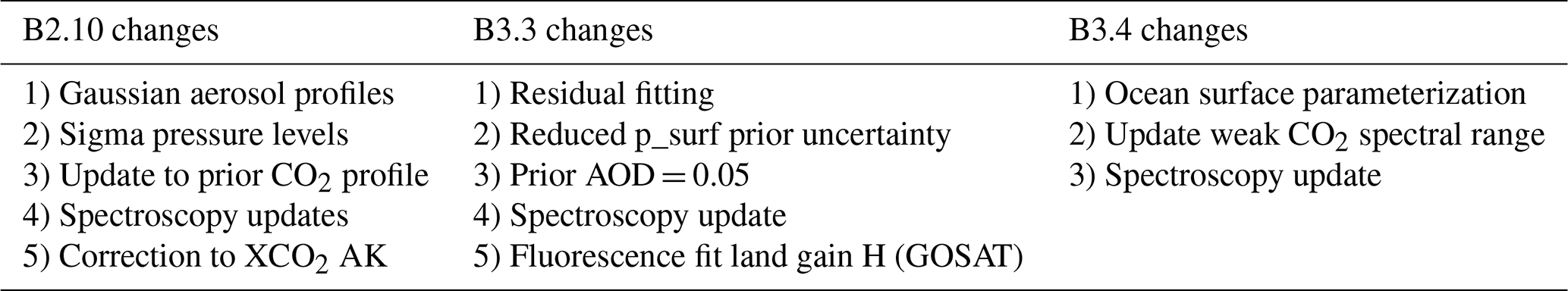
Although newer versions of the OCO-2 L2 algorithm exist (currently b8 as of time of writing), the work presented here was initially begun prior to the launch of OCO-2 in July 2014. In addition, certain tests, where the L2 true state is directly related to the retrieval vector, were simplified by using the older version of the retrieval algorithm which contains a less complicated aerosol scheme. In the older L2 algorithm versions (pre-B3.5), also used in this work, the state vector for all soundings always included the same four aerosol types: cloud water, cloud ice, Kahn 1 (a mixture of coarse- and fine-mode dust aerosols), and Kahn 2 (carbonaceous-mode aerosols) (described more in Nelson et al., 2016). Both Kahn 1 and 2 types contain some sulfate and sea salt aerosols as well. Newer versions of the OCO-2 L2 retrieval include a more complicated scheme in which each sounding includes water and ice, and they pick the two most likely aerosol types based on a MERRA monthly climatology for the particular sounding location. The aerosol fits use a Gaussian-shaped vertical profile for each of the four types, as described in O'Dell et al. (2018).
Inputs to the b3.4 L2 retrieval algorithm include simulated L1b radiances and meteorology (taken from ECMWF) that were generated using the CSU/CIRA simulator (O'Brien et al., 2009). The simulator is driven by satellite two-line elements which are used to provide the satellite time and position. The code calculates relevant solar and viewing geometry and polarization and takes surface properties from MODIS. Only a single day's worth of orbits (15 orbits on 17 June 2012) at reduced temporal sampling (1Hz instead of the operational 3 Hz) and with only one footprint per frame (instead of the operational eight) is presented in this work. This yields approximately 2700 soundings per orbit, totaling about 40 000 soundings. Unlike real OCO-2 viewing modes (see Crisp et al., 2017), the simulations were generated with nadir viewing over land and glint viewing over water. Our simulations do not include nadir-water, glint-land, or target mode simulations, which are additional observation modes used in real OCO-2 data (Crisp et al., 2017). The spectral error for these simulations assumes Gaussian random noise, following the OCO-2 noise parameterization as described in Rosenberg et al. (2017).
Although the simulations do include realistic clouds and aerosols from a CALIPSO/CALIOP (Winker et al., 2010) monthly climatology, the radiative transfer portion of the simulator code allows clouds and aerosols to be switched off, making it easy to generate clear-sky radiances used in this research. The OCO-2 instrument model, described in detail in O'Brien et al. (2009), was used to add realistic instrument noise to the radiances prior to running the L2 retrieval for the noiseless simulations. The operational OCO-2 dispersion, instrument line shape (ILS), and polarization sensitivity were used to sample the top-of-atmosphere radiances. The same solar model as used in the operational retrieval was used in the L1b simulations. In addition, the A-band preprocessor code described in Taylor et al. (2016) was run on the cloudy-sky L1b simulations to provide realistic cloud screening prior to running the L2 retrieval. It is important to test the system from end to end with radiances containing a variety of cloud conditions, because the cloud screening is never 100 % accurate, sometimes letting through cloudy cases, and because quality flags can sometimes flag cloudy cases being as good quality without clouds.
This error analysis ideally would use the exact same forward model in both the L1b simulations and the L2 retrieval algorithm, as our analysis assumes that Eq. (1) should be valid, without errors from forward model differences. However, in reality these two code bases are very similar but not identical. For example, the number of vertical levels within the two code bases differs. Reasonable attempts were made to put the L1b simulations on the same footing with the L2 forward model, but minor model mismatches may remain. We do not believe these minor differences affect our primary results.
Our goal in this work is to compare linearly predicted vs. actual errors in XCO2, specifically in terms of three primary contributions to the retrieval error discussed above: measurement, smoothing, and interferent error. Several different configurations were used to allow the estimation of the true error for each of these error components, as shown in Table 3. The clear results have no clouds or aerosols in the true state; however, the retrieval is free to insert clouds into the retrieved state (and given that aerosols are retrieved as ln(AOD), the retrieved states is never fully aerosol-free).

Results from different configurations are intercompared to validate the individual measurement, smoothing, and retrieval errors. These predicted errors are compared to the true errors resulting from nonlinear retrievals, which are the retrieved minus true values.
2.3 Postprocessing quality screening
Similar to retrievals from real observations, the simulated retrieval results need screening to remove cloudy scenes (e.g., see O'Brien et al., 2016; Polonsky et al., 2014). Because prescreening is not perfect, the XCO2 estimates from some soundings are of low quality, even if they converge. Postprocessing screening is handled through calculation of quality flags, taken from Table 5 of Polonsky et al. (2014). These flags are (a) (defined in Eq. 6) < 2 for cases with measurement error or < 1 for cases with no measurement error, (b) retrieved aerosol optical depth < 0.2, and (c) degrees of freedom > 1.6 (degrees of freedom are defined near Eq. 4). The three bands are averaged to calculate the for the scene.
Table 4Number of cases for each configuration. The clouds in true = yes cases contain many fewer soundings than no clouds because of prescreening. The no. good is from postprocessing screening.
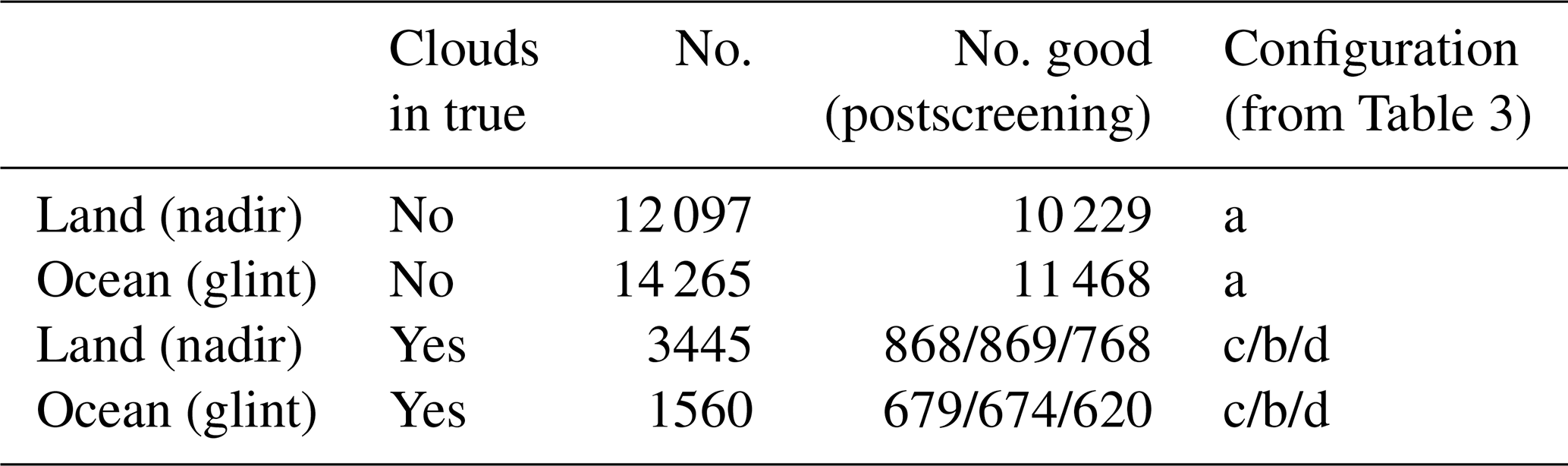
Table 4 shows the effects of applying postprocessing quality screening for the different configurations from Table 3. The results are separated into land and ocean scenes; approximately one-third pass postprocessing quality screening for cloudy cases; about 80 % pass postprocessing quality screening for cloud-free cases. For configuration (c) in Table 3 (simulations that include clouds), 11 % and 28 % of cases passing prescreening for ocean and land, respectively. Post-processing screening identifies 25 % and 43 % of cases for ocean and land, respectively. These are low compared to OCO-3 simulation studies (Eldering et al., 2019), where 25 %–30 % of cases passed prescreening and 50 %–70 % of cases passed postscreening. Some of the quality flags used for the OCO-3 studies (particularly the preprocessing flags) are not available in our study, so it is hard to directly compare throughput. The lower throughput suggests that the cloud cases or other aspects of this study were harder than the OCO-3 simulation studies.
2.4 Comparisons of retrieved values to true
Table 5 shows XCO2 biases and errors for the different configurations from Table 3. The quantities calculated for Table 5 are the bias (the mean retrieved minus true values) and standard deviation (the square root of the second moment of the retrieved minus true difference). These quantities indicate the overall quality of the results for each configuration. The results in Table 5 are sorted by standard deviation. The worst result by far is the cloudy case with no postprocessing screening. This has ∼10 ppb error for land and ∼3 ppm error for ocean. Ocean generally does better than land, postprocessing screening generally does better than no screening, and clear cases do better than cloudy cases. The addition of measurement error has a negligible effect on standard deviation for this testing. The bold entry in Table 5 represents the most realistic real-life case (+ measurement error, + clouds, + postprocessing screening). This has 0.8 ppm standard deviation for land and 0.7 ppm standard deviation for ocean.
Table 5Mean bias and standard deviation between retrieved and true, sorted by standard deviation. The bold entries are the nominal cases most closely simulating actual OCO-2 retrievals.
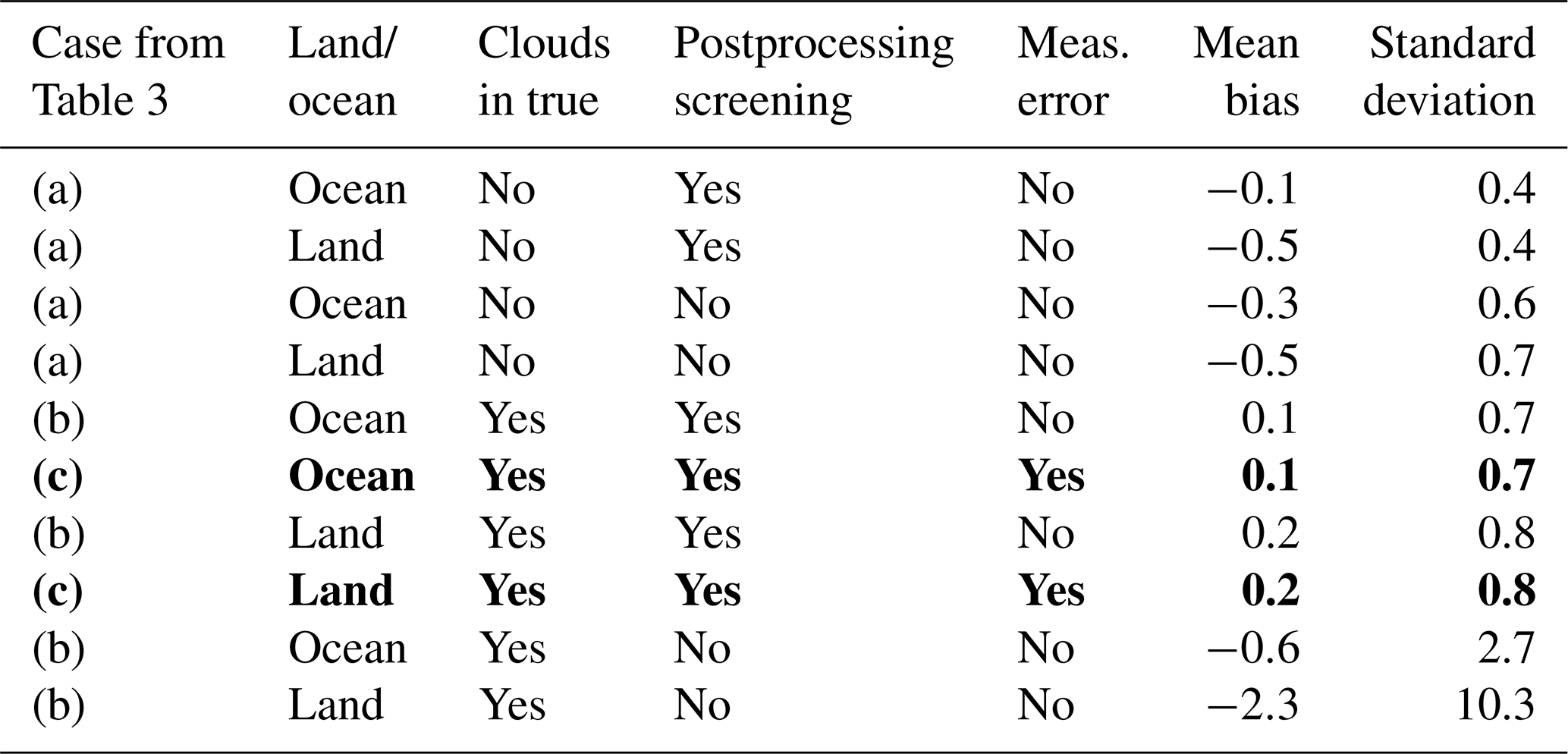
In the screened data, the main concern is the −0.5 ppm bias in the clear land retrieval. We have seen this in other sets of simulations and it is an unresolved issue at this time. Recently we did find a minor bug in the simulator code that caused a small mismatch between the water vapor profile used to calculate the L1b radiances and that written to the meteorology file that is then used in the L2 retrieval. It is possible that other minor bugs of this nature are driving the clear-sky bias, with errors mitigated by clouds in the cloudy cases.
Figure 1 shows a scatter plot of the retrieved versus true XCO2 (both with the a priori subtracted). The lower panels in Fig. 1 show the histogram of differences, which range from about −1.25 to +1.5 ppm for land and −1.5 to +2 ppm for water soundings. Bias correction, discussed in Sect. 4.3, further improves the land results by 0.1 ppm in the bias and standard deviation as seen in Table 5 but does not improve ocean results. The standard deviations of (retrieved – true) (green dashed line) and (retrieved – linear estimate) (blue dashed line) are very similar; the linear estimate does not estimate the results any better than 0.7 to 0.9 ppm and gives an estimate of the nonlinearity.
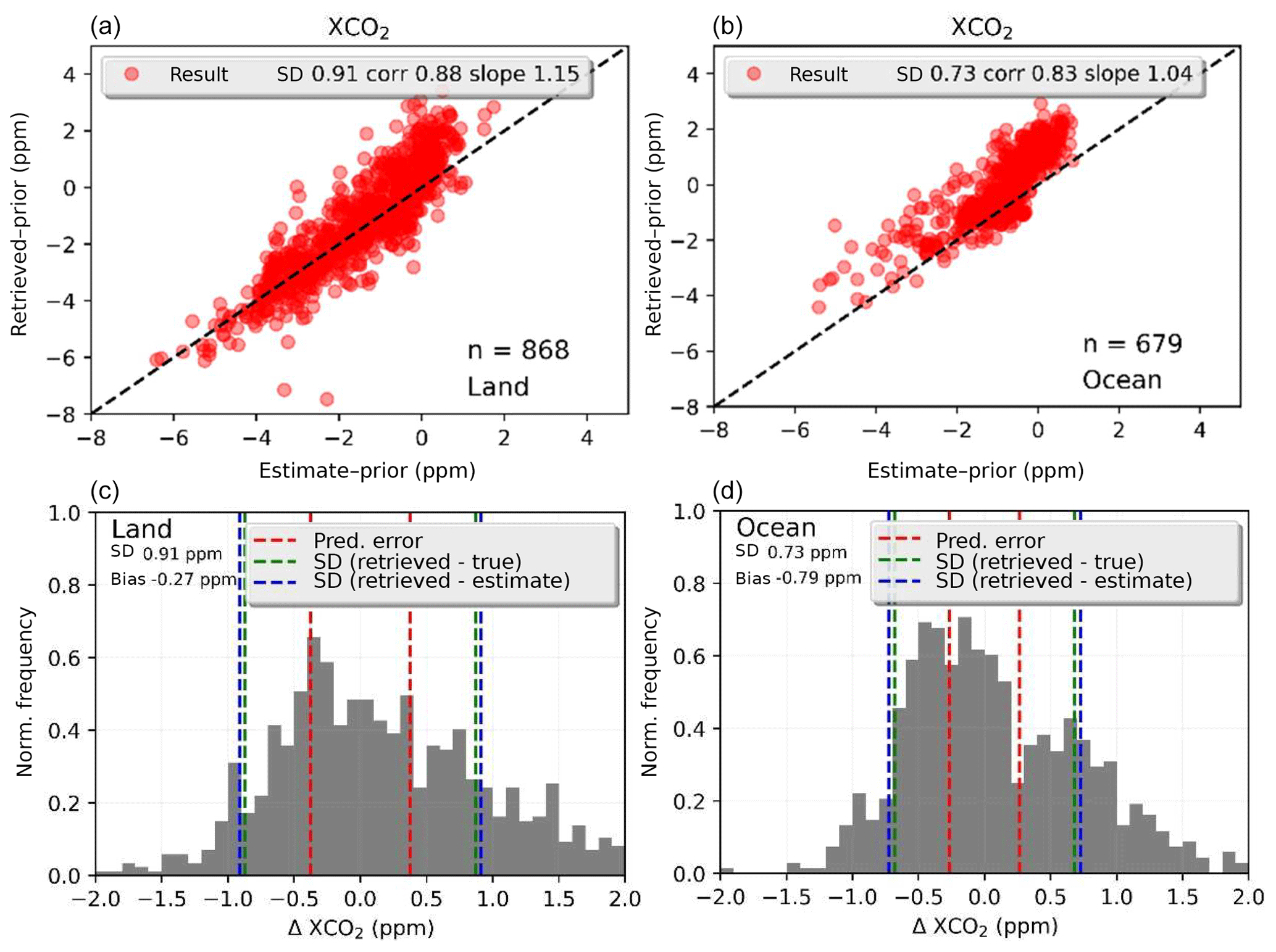
Figure 1Scatter plots of XCO2 difference from the prior for retrieved versus true on the simulated data. This corresponds to dataset (c) with clouds and measurement error; postprocessing screening applied for land (a, c) and ocean (b, d), with 1:1 plots shown in panels (a) and (b); and histogram of the differences in (c) and (d).
For real OCO-2 v8 data, comparisons to TCCON for single-observation land nadir and ocean glint have errors of 1.0 and 0.8 ppm, respectively (Kulawik et al., 2019a), meaning that the real errors are comparable to these simulated data. Real OCO-2 data have a systematic error on the order of 0.5–0.6 ppm (Wunch et al., 2017; Kulawik et al., 2019a). Correlated biased errors are seen in real OCO-2 data, with correlations in time, e.g., ∼60 d (Kulawik et al., 2019a), at small spatial scales, e.g., < 1∘ (Worden et al., 2017), and at medium spatial scales, e.g., 5–10∘ (Kulawik et al., 2019a). Although this dataset cannot probe a seasonally dependent bias, as it covers only 1 d of observations, it can be used to probe spatial patterns of the biases. However, note that probing very small spatial patterns will be difficult to see because of the small number of data processed in comparison to real OCO-2. A plot showing the spatial pattern of retrieved minus true is shown in Fig. 2a, which shows a high bias near the Equator and a low bias near the poles. Figure 2b shows the difference between true XCO2 and XCO2 with the OCO-2 averaging kernel. The overall spatial pattern in panel (a) is not affected by the application of the averaging kernel, which makes sense because the averaging kernel effect is ∼0.2 ppm, whereas the differences are on the order of 0.9 ppm. An analysis of the correlation scale length of (retrieved minus true) XCO2 finds a correlated error of 0.3 ppm and the full width at half maximum in the bias of ∼3∘, which is similar to the correlated error of 0.4 ppm and scale length of ∼5–10∘ found in Kulawik et al. (2019a). The simulated data have an accurate meteorology (temperature, winds, etc.) that drives the simulated true states, but the cloud and aerosol spatial structures are not very accurate, so that the spatial scales are not expected to be identical between this simulated dataset and real OCO-2 data. This analysis shows that correlated biases exist in simulated data and that simulated data are useful for exploring the characteristics and, even more importantly, the cause of regional biases.
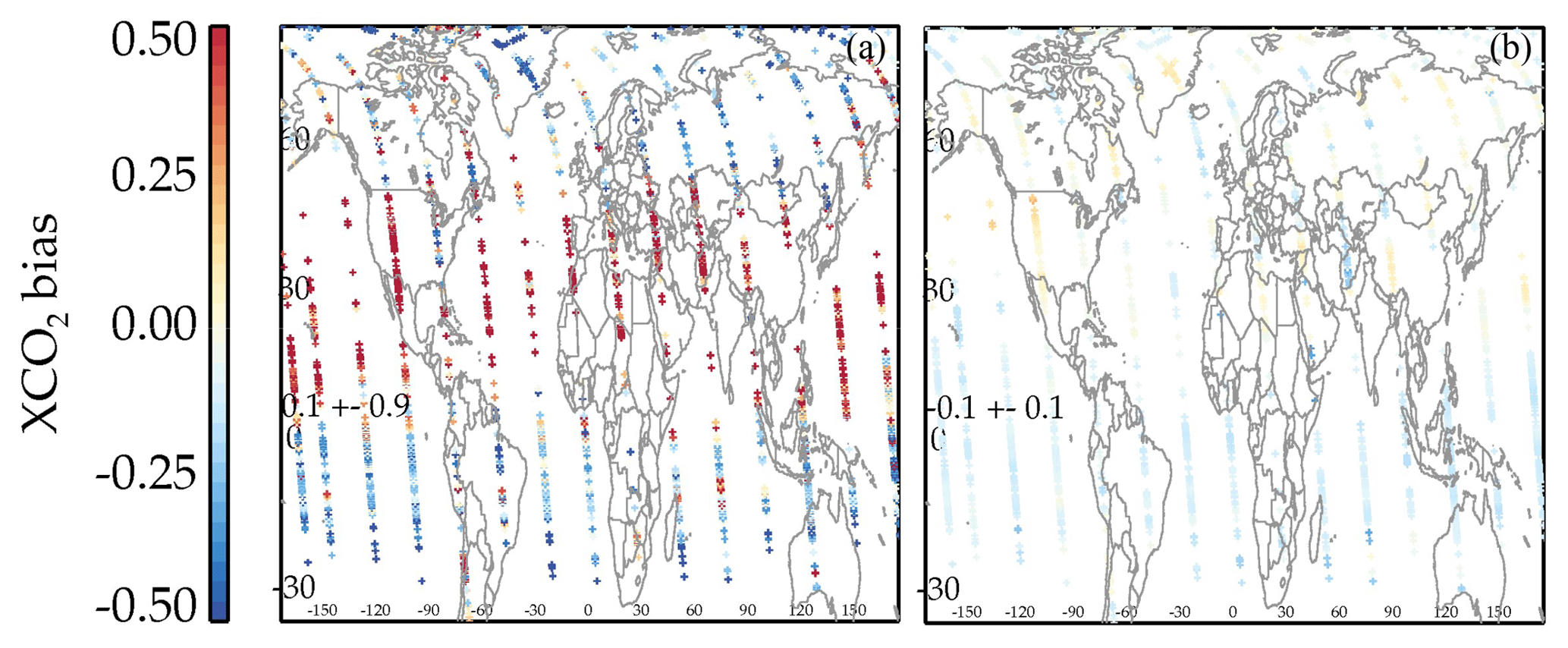
Figure 2(a) Spatial pattern of XCO2 retrieved minus true for case (b) from Table 3 (cloudy but no measurement error), with quality screening. Panel (b) shows the difference between true XCO2 with the OCO-2 averaging kernel applied minus true XCO2.
In this section the different error components that were introduced in Sect. 2.1 are isolated as much as possible to evaluate each one separately. The averaging kernel and Jacobians, introduced in Sect.2.1, are used as diagnostics. In addition, the linearity, or lack thereof, of the system is explored.
3.1 System linearity
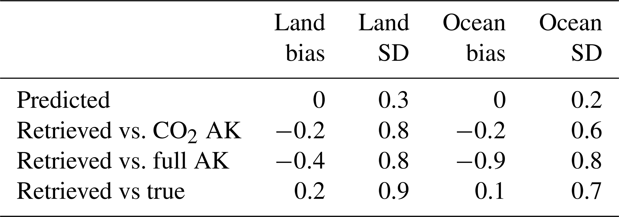
To test the system linearity the linear estimate, using Eq. (1) and discussed in Sect. 2.1 is compared to the nonlinear retrieval result. The inputs to Eq. (1) include the instrument noise (if on), a priori covariance, and Jacobians at the final retrieved state. Table 6 shows the results for cases passing postprocessing quality screening, clouds, and no measurement error (Table 3, case d) using (1) the first two terms on the right side of Eq. (1) (i.e., only the CO2 part of the averaging kernel) or (2) all of Eq. (1) (i.e., utilizing the interferent terms). The last term of Eq. (1) is not used for the noise-free case. The bottom entry in Table 6, shows the retrieved vs. true XCO2 (without averaging kernel applied). The comparisons of retrieved XCO2 versus the linear estimate have biases between 0.2 and 0.9 ppm and standard deviation between 0.6 and 0.9 ppm. The bias is worse if the full averaging kernel is used. Looking through parameter by parameter, the band 3 albedo average causes most of the large bias for the full averaging kernel for ocean. The difference between the linear estimate and the nonlinear retrieval is an estimate of the nonlinear error in the retrieval system.
Table 6Difference of linear estimate versus nonlinear retrieval, noise-free, cloud, quality-screened cases. SD denotes standard deviation.
Another test of the system linearity is the consistency of the sensitivity of the system to changes in XCO2; i.e., how constant are the XCO2 Jacobians (defined in Eq. 3)? For example, consider if the XCO2 Jacobian weakens when an interferent, e.g., call it interferent no. 1, increases. If interferent no. 1 is larger than its true value, the XCO2 Jacobian will be weaker than the true XCO2 Jacobian. If the XCO2 Jacobian is weaker than the true Jacobian, then more XCO2 is needed to account for the radiance differences observed, resulting in a positive bias in XCO2. This would result in a positive correlation in the errors of interferent no. 1 and XCO2. This error correlation would not be predicted by the linear error analysis because the linear error analysis assumes that the Jacobians do not vary. This could explain the stronger error correlations seen.
To calculate an error resulting from varying Jacobians requires calculating second-order terms, like dJacobian[XCO2]∕d[H2O scaling]. Cressie et al. (2016) calculated nonlinear errors, using second-order error analysis, and found errors on the order of 0.2 ppm, which would not fully explain the discrepancy between the predicted and true errors either in the simulation studies or real data.
Figure 3 shows the Jacobian magnitude (the XCO2 Jacobian averaged over all frequencies) for XCO2 versus retrieved band 2 albedo slope. The Jacobians for the lower (LMT) and upper (U) partial columns (described in Kulawik et al., 2017, and Sect. 2.1) are also plotted, and both partial columns vary the same way, e.g., same slope signs; i.e., the nonlinear interferent error would be positively correlated between the two partial columns.
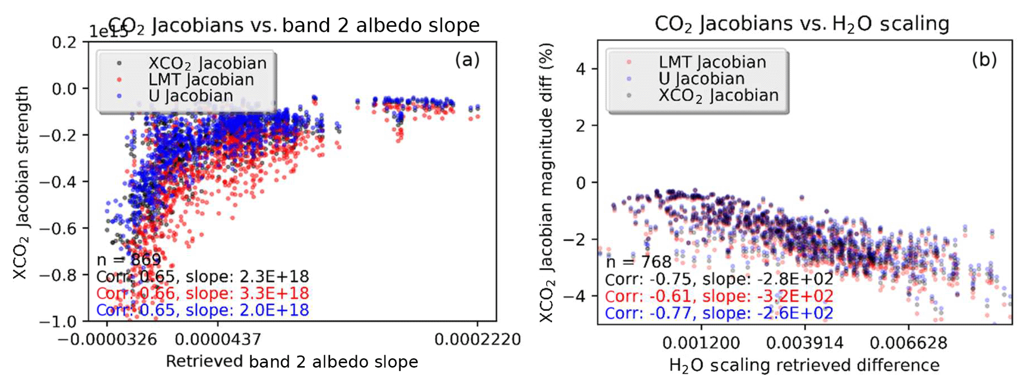
Figure 3XCO2 (black), lower CO2 partial column (red), and upper CO2 partial column (blue) Jacobian band-averaged magnitude versus interferent parameters. (a) shows CO2 magnitude versus retrieved band 2 albedo slope, using the configuration (b) from Table 3; (b) shows the CO2 Jacobian magnitude difference (in percent) for matched cases from run (b) and (d) versus differences in retrieved H2O scaling.
The right panel of Fig. 3 compares the Jacobian magnitude between matched results from configuration (c) and (d) in Table 3 for land cases with postprocessing screening. The CO2 Jacobian magnitude difference is up to −4 % for case (c) minus (d) and is correlated with the difference in retrieved H2O scaling with correlation −0.75. Other parameters that had strong correlations (> 0.4) are aerosol water pressure (0.55), aerosol ice pressure (0.43), surface pressure (0.41). Mapping this correlation to an error in retrieved XCO2 would require the calculation of second-order Jacobians as in Cressie et al. (2016) and then mapping this into an error in XCO2. A crude way to estimate the XCO2 error resulting from these Jacobian differences is to consider the completely linear case, where radiance is equal to K multiplied by XCO2. In this case, a +1 % error in the Jacobian would result in a −1 % error in XCO2, to fit the radiance. So, the variations in the XCO2 Jacobians that are seen could explain the 0.8 ppm XCO2 differences from the linear estimate.
3.2 Measurement error
To validate the measurement error, results from runs with and without noise (cases (c) and (b) from Table 3) are analyzed. The standard deviation of the XCO2 difference between the runs (true error) was compared to the predicted measurement error. The two runs, which both have clouds and other interferents, as well as smoothing errors, are assumed to be identical other than one having measurement error added. The runs are compared after quality screening, which was described in Sect. 2.4.
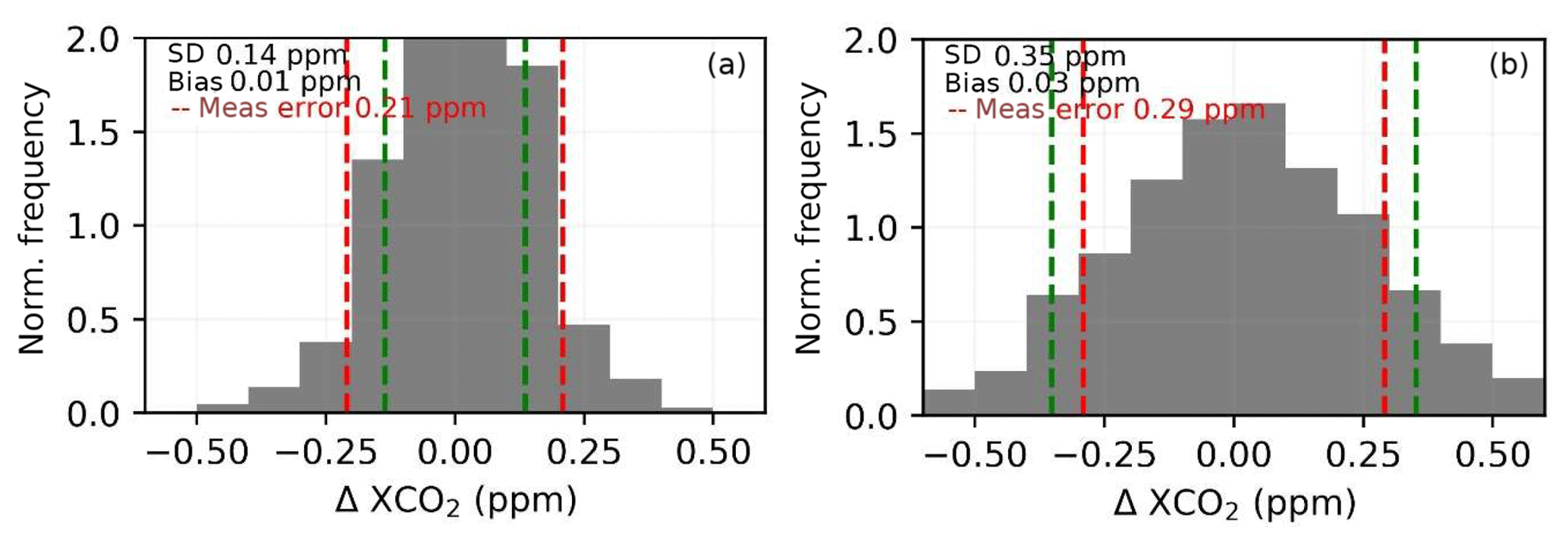
Figure 4Histogram of difference between XCO2 with noise on and noise off for ocean (a) and land (b), cases (b) and (c) from Table 3.
Figure 4 shows the baseline and predicted measurement error. For land nadir, the average error is 0.35 ppm and the average predicted is 0.29 ppm. For ocean glint, the average error is 0.14 ppm and the average predicted error is 0.21 ppm. The bias difference between the runs with and without noise was 0.01 ppm for ocean and 0.03 ppm for land nadir.
The predicted error ranged from 0.14 to 0.70 ppm for land and 0.12 to 0.35 ppm for ocean. The correlation between the predicted error and the absolute value of the error is 0.27 for land and 0.08 for ocean, so the scene-to-scene variations in the predicted error are not very useful.
Adjacent observations are averaged, and then the error of this averaged quantity is calculated. If the error reduces with the square root of the number of observations averaged, then the error is a random, not correlated, error. A random error is highly desirable for assimilation and other uses. For land nadir the error is shown in Table 7.
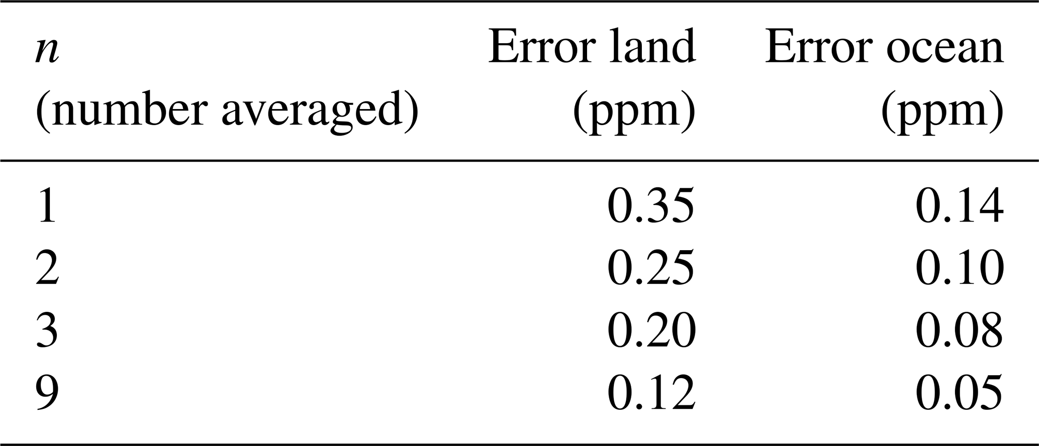
If the error is random, then the n=9 result should be one-third of the error for the n=1 result, and this is what is found. Similarly for ocean, the error for n=9 is 1∕3 of the n=1 error. The simulated data do not have the data density of actual OCO-2 data, so while averaging in close proximity would likely behave similarly, there is some uncertainty.
In summary, for these simulated cases, the measurement error is overpredicted for land by 0.06 ppm and overpredicted for ocean by 0.07 ppm, but the measurement error appears to average randomly and does not introduce a bias.
3.3 Smoothing error
Smoothing error occurs when the averaging kernel deviates from the identity matrix, and it is calculated using the averaging kernel, the true state, and the prior state. The smoothing error terms from Eq. (1) are
Here, v represents the CO2 profile, which is converted to XCO2 using Eq. (5). To validate the smoothing error, the nonlinear retrieved XCO2 is compared to the linear estimate, , from Eq. (7), and to . The linear estimate should compare better to the nonlinear retrieval. Run (a) from Table 3 is used, which does not contain clouds in the true state (i.e., limited interferent error) and does not have a measurement error in the observed radiances.
The predicted smoothing error is 0.12 ppm for ocean glint and 0.16 ppm for land nadir. Comparison between retrieved XCO2 and true has a mean bias of 0.0 ppm for ocean and a mean bias of 0.46 bias for land (retrieved XCO2 is 0.46 ppm lower than true). The standard deviation is 0.33 ppm for land and 0.35 ppm for ocean.
Comparison of the retrieved XCO2 versus (XCO2)true_ak or (XCO2)true yielded the same biases and standard deviations (within 0.02 ppm). Therefore, the use of the OCO-2 averaging kernel and prior for comparisons, using Eq. (7), does not improve the comparison quality versus OCO-2. This analysis suggests modelers would get similar quality results whether or not the OCO-2 averaging kernel is applied during assimilation. However, a previous study by Wunch et al. (2011) found that for comparisons to TCCON, if the averaging kernel is not applied, it leads to 0.2 ppm seasonal biases. The current analysis shows that it does not do harm to apply Eq. (7) but that it does not help either, with the caveat that the simulated data do not cover different seasons.
3.4 Interferent error
Previous studies by Merrelli et al. (2015) and O'Brien et al. (2016) have found that clouds and aerosols can contribute errors larger than predicted. We look at the relationship between errors in retrieved interferents versus errors in XCO2 and the prediction of the relationship as characterized by the averaging kernel.
The error in XCO2 from the interferent term of Eq. (1), multiplied by the pressure weighting function, h, estimates the propagation of interferent error into XCO2, shown in Eq. (8).
This equation predicts that the interferent will only have an impact if the prior state is different than the true state and that the impact will be proportional to the prior state minus the true state difference, with the constant of proportionality provided by the off-diagonal averaging kernel, Axv. Many of the interferents, e.g., H2O Scaling, start at their true values for this simulation and therefore are predicted to have no impact on XCO2 errors. Yet, large correlations in errors are seen when comparing XCO2 errors and interferent errors, e.g., H2O Scaling error. Taking the expected standard deviation of the XCO2 interferent error from Eq. (8) gives the predicted interferent error, which averages 0.2 ppm for case (b) from Table 3.
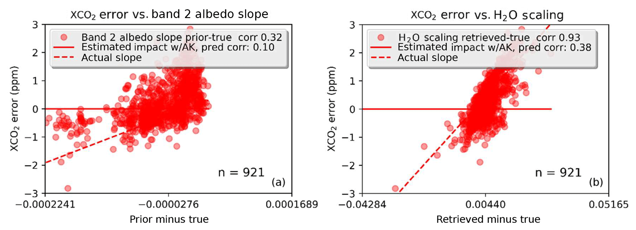
Figure 5Predicted (red line) and true error (red dots) for two interferents: band 2 albedo slope (a) and H2O scaling (b).
We look at (retrieved minus true XCO2) versus (prior minus true interferent) or (retrieved minus true interferent) in Fig. 5, using run (b) from Table 3, which has clouds but no measurement error. The red line shows , the predicted relationship between the XCO2 error and the prior minus true difference. For both band 2 albedo slope, left, and H2O scaling, right, there is no predicted relationship, but a strong correlation is seen. This could be explained by the results from Sect. 3.1, showing that the XCO2 Jacobian strength varies with the retrieved albedo or retrieved water, whereas the error analysis assumes that the Jacobian strength does not vary.
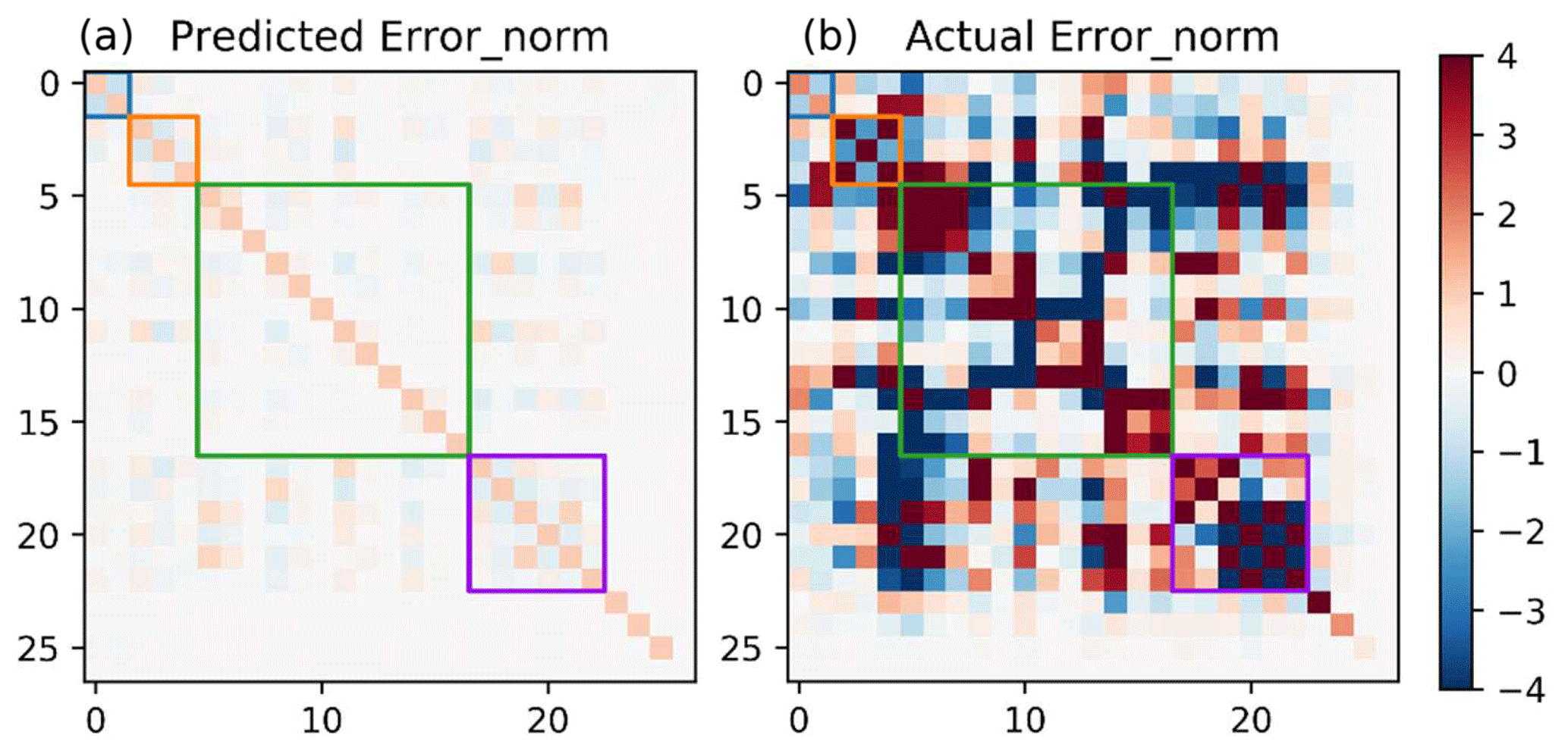
Figure 6Predicted and true errors. (a) shows the predicted error covariance matrix, for the retrieval parameters listed in Table 1, with the CO2 profile collapsed into two parameters (LMT and U partial columns). The blue, orange, green, and purple boxes contain CO2, metrological, aerosol, and albedo parameters, respectively. Both matrices are normalized by the diagonal of the predicted errors.
Figure 6 shows the predicted versus true errors, including correlations. The true error is calculated from for all cases with good quality. The true errors are much larger and show more correlations than predicted. Both matrices are normalized using the equation , where Error is the error covariance of interest and Error0 is the predicted error covariance. To further analyze the interferent error, we looked at the diagonal terms of the error covariance and the correlations to XCO2 in Table 8. In order for the error correlations between XCO2 and interferents to be assessed, the CO2 profile is mapped to XCO2 using Eq. (5). Table 8 shows the predicted and true errors for all interferents, for all good-quality land cases. The error factor (EF) is calculated as
where the predicted standard deviations come from the predicted errors and the true standard deviation and bias come from the true errors. The error factor is found to be greater than 1 for almost all parameters.
Table 8Predicted and actual errors for interferents and correlations between interferents and XCO2 for simulated land retrievals for case (b) from Table 3. Bold values are those parameters with interferent errors larger than predicted and large actual correlations to XCO2 error (absolute value larger than 0.25).
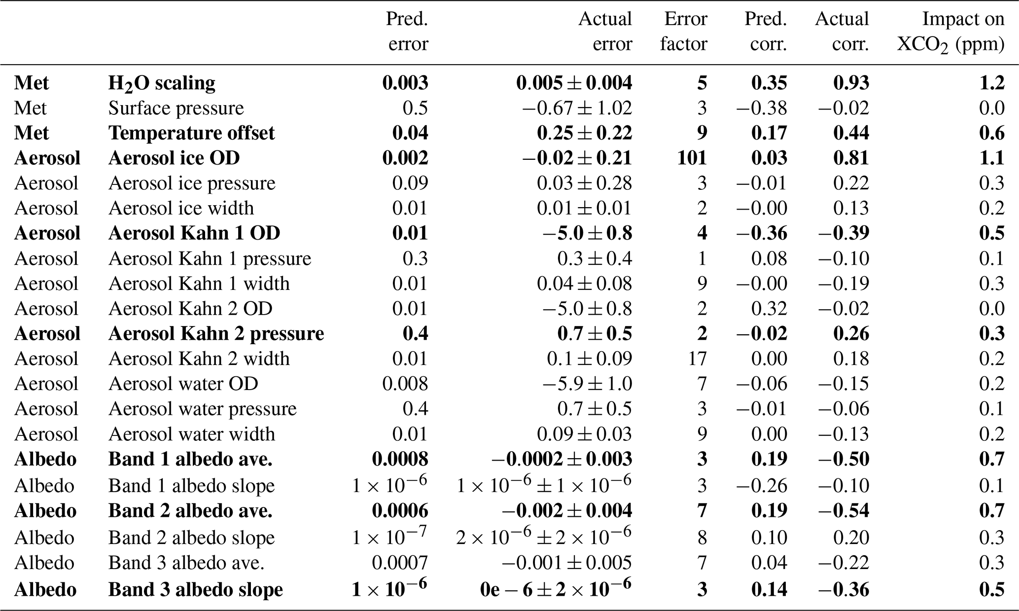
Another useful diagnostic of interferent error is the predicted error correlation between each interferent and XCO2, calculated by
which can be compared to the actual error correlation. Table 8 shows that for most interferents both the errors and the correlations are underpredicted. The parameters that are both underpredicted and significantly correlated (> 0.25) to XCO2 errors are shown in bold.
The true effect of interferent error on XCO2 can be crudely estimated by the actual slope of XCO2 error (not shown in Table 8s, but the actual slope is shown in Fig. 5) multiplied by the interferent error. This estimate cannot distinguish between correlation and causation. The standard deviation of this estimate is shown as the last column of Table 8 (“Impact on XCO2”). The interferent error estimated with a more simplified surrogate model was much smaller in Hobbs et al. (2017).
Postprocessing analysis of real ACOS OCO-2 retrieval results has uncovered linear relationships between XCO2 error and various parameters such as the retrieved surface pressure, liquid water optical depth, and (an estimate of the profile curvature) (Wunch et al., 2011). Similar correlations have been found between the above parameters and the lower partial column (Kulawik et al., 2017). The standard operational procedure that has been adopted by the ACOS algorithm team for both OCO-2 and GOSAT data is to perform a bias correction of the estimated XCO2 based on the linear correlations of the difference in XCO2 compared to various truth metrics with certain retrieved parameters. In this section, we look specifically at the behavior of (defined in Sect. 4.1) and dP (defined in Sect. 4.2) bias correction in the simulated system. The purpose of the analysis of this section is to answer the following questions.
-
Do the bias correction for dP and behave similarly in the simulation system to the real OCO-2 retrievals?
-
What is the effect of bias correction on CO2 errors?
The bias correction is determined using this simulated dataset and then applied to the same dataset, which is somewhat circular, since the true is both used to determine the bias correction and to check the bias correction, but it is important to know whether the relationships exist. For example, what causes the spatial patterns seen in the bias in Fig. 2.
4.1 The retrieved profile gradient
is defined as delta[20]–delta[13] , where delta is the retrieved CO2 profile minus the prior CO2 profile, [20] is the surface level, and [13] is seven levels above the surface, i.e., 0.63*(surface pressure). represents the gradient of the retrieved CO2 profile that differs from the prior. It has been found that the slope of XCO2 error versus varies depending on the a priori covariance that is used in the retrieval system, with a more evenly varying covariance having less dependency of XCO2 error versus (O'Dell, unpublished data). The standard OCO-2 constraint is very loose at the surface (e.g., with 50 ppm a priori variability) and tighter in the midtroposphere (with ∼10 ppm a priori variability). Most CO2 variability does occur near the surface near the primary sources and sinks, but the a priori constraint used in the retrieval algorithm would favor variations at the surface even in cases when the variations occur at a higher level due to the weighting due to the prior covariance.
Figure 7 shows errors in XCO2, LMT (the lower tropospheric column, approximately up through 2.5 km), and U (the upper partial column, approximately from 2.5 km through the top of the atmosphere) (LMT and U are described in Kulawik et al., 2017, and Sect. 2.1) versus for configuration (b). In the simulated retrievals, the values of the slope of delta XCO2 versus are −0.001 and −0.008 for land and ocean, respectively. It is clear that there are significant errors in the partitioning between the lower (LMT) and upper (U) partial columns that are correlated to . The slope of LMT versus is 0.23 and 0.22 for land and ocean, respectively, and −0.07 and −0.08 for U land and ocean, respectively. For real ACOS-GOSAT (B3.5) data, Kulawik et al. (2017) found a slope of 0.39 for land and 0.31 for ocean for LMT and −0.11 and −0.09 for U land and ocean, respectively, which are similar values as seen in this simulated dataset.
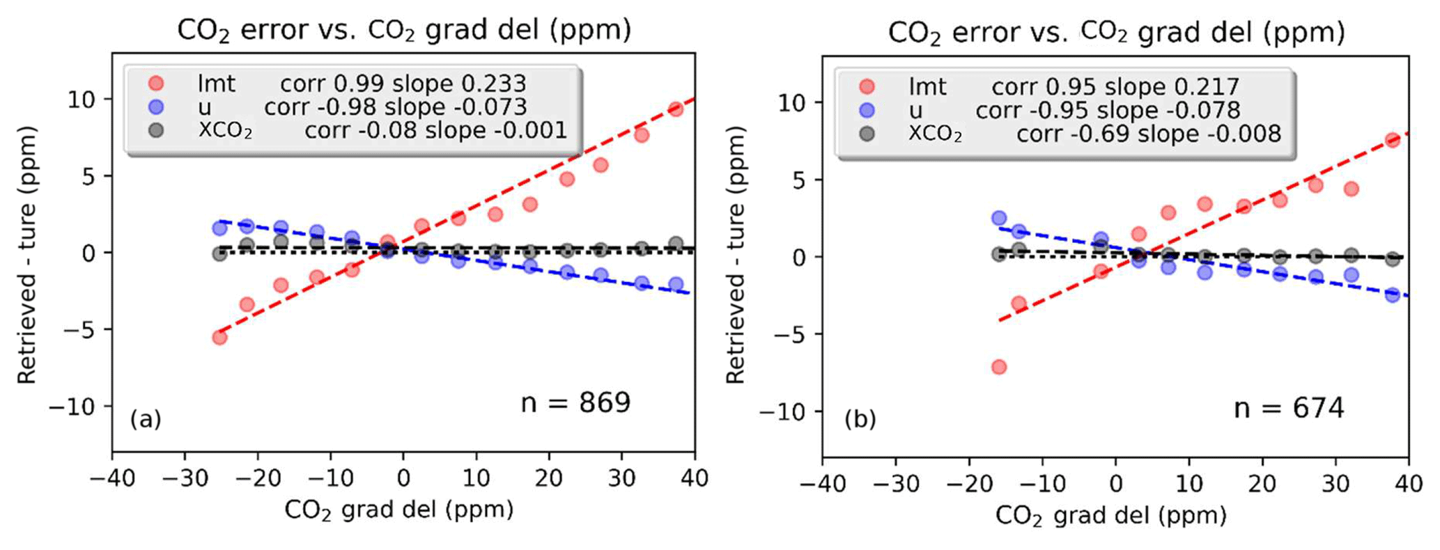
Figure 7Error in retrieved CO2 for XCO2 (black), upper partial column, U (blue), and lower partial column LMT (red) versus for ocean (a) and land (b).
These results naturally lead to the following question: what is the effect of placing CO2 at the wrong pressure level? The mean Jacobian for the U partial column (upper 15 layers) is only about 60 % (0.62) of the mean value for the lowermost four layers. Therefore, a molecule in the LMT partial column is equivalent to about 1.6 molecules in the upper partial column. Therefore, a molecule mistakenly placed in the lower four layers and moved to the upper layers in the postprocessing step needs to be exchanged for 1.6 molecules in the upper partial column to have the same impact on the radiances at the new level. At of 35, for land, LMT is high by ∼8.4 ppm. For an even exchange, moving 8.4 ppm from the LMT partial column to the U partial column results in +2.5 ppm in the U partial column only from the effects of air mass (because the U partial column has more air mass; =8.4 ppm *.23 LMT air mass/0.77 U air mass). Considering the difference in sensitivity, and multiplying by 1.6, this corresponds to +4.0 ppm in the U partial column. The net effect on XCO2 of this bias correction is the sum of the partial columns times the air mass, ppm. This is at of 35, so that would mean that the slope for XCO2 error versus is 0.031. For real OCO-2 v7 data, the slope of XCO2 error versus is +0.0280 and −0.077 for land and ocean, respectively (Mandrake et al., 2017). This analysis explains a positive slope in XCO2 versus but would not explain a negative slope. The negative slope would result from additional correlations or errors acting in addition to this effect.
4.2 The retrieved surface pressure
The quantity dP is the difference between retrieved and prior surface pressure and is used as a postprocessing bias correction for OCO-2. In this section, we explore results from dP in the simulated dataset to try to understand why bias correction based on this parameter is useful.
Although it is typically assumed that the surface pressure is determined solely from the O2 A band, the strong and weak CO2 bands also contribute information. For land nadir, averaged over cases passing postprocessing quality screening, the band-averaged Jacobian strengths in the weak and strong CO2 bands relative to the O2 A band are 0.2 and 0.4, respectively. Based on the surface pressure Jacobian and the spectral error, a value of −2 hPa will create a spectral bias 0.2 times the size of the spectral error in the O2 A band, which, because it is a correlated error, will be an additive error over the band.
Figure 8 shows the actual error covariances and biases for three different subsets of run (d): dP < −2 hPa, hPa (nominal cases), and dP > 1.5 hPa. The errors shown are normalized by the predicted error, using the equation , where E is the error covariance of interest and E0 is the predicted error covariance. A diagonal value of 1 means that the actual error is the same as predicted, and a diagonal value of 4 represents an actual error that is twice () as large as predicted. The errors and error correlations are much larger than predicted for many parameters. In addition, the CO2 parameters show less correlation with other parameters for the nominal case. Also note that the nominal case has less saturation, meaning less errors and correlations.
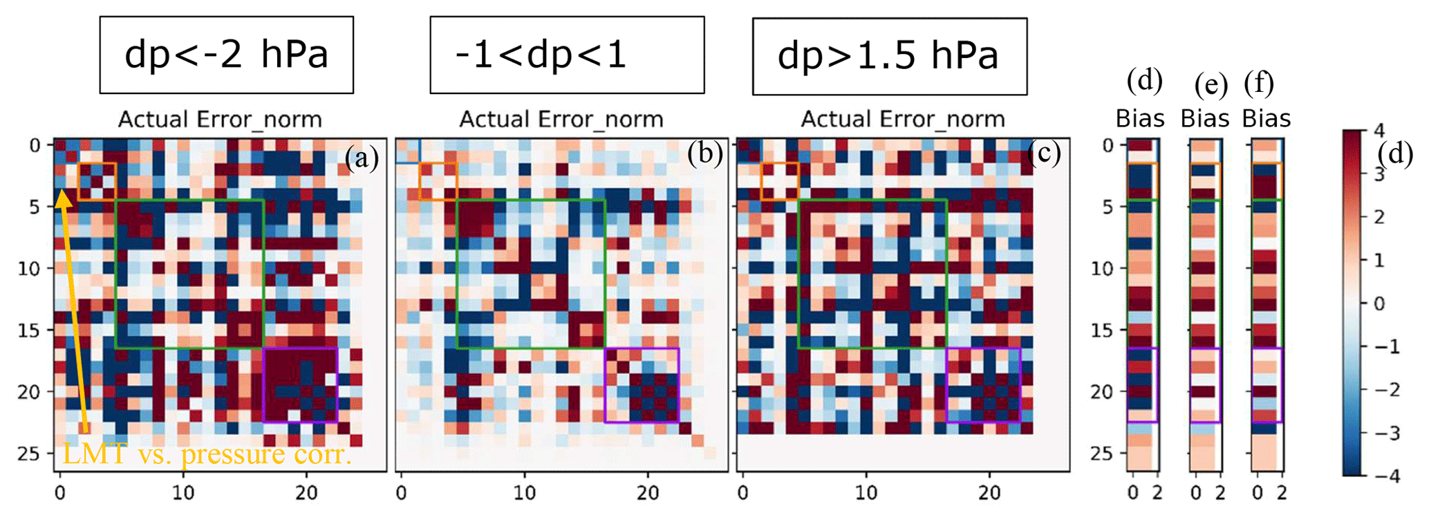
Figure 8Normalized actual error covariances and biases of retrieved parameters for dP < −2 hPa (a, d), −1 < dP < 1 hPa (b, e), and dP > 1.5 hPa (c, f) using the configuration from Table 3 (d) for land/cloudy. The purple box surrounds the albedo parameters, the green box surrounds aerosol parameters, the red box surrounds metrological parameters, and the blue box surrounds the CO2 fields, which have been collapsed into lower and upper partial columns. The errors are normalized by the predicted errors (which are shown in Fig. 5). The arrow in panel (a) shows correlation between LMT and surface Pressure, which is negative (also see Fig. 9b below).
Next we looked at the possibility of screening incorrect surface pressure results using (defined in Eq. 6). To do this, we used land cases for configuration (c) in Table 3 (simulations that include clouds), and looked at for two groups: (group 1) dP < −2 and (group 2) −1 < dP < 0. The cases with dP < −2 had 0.04, 0.01, and 0.06 higher reduced in the three bands, respectively. Although the dP < −2 case fit the spectra worse there was too much overlap to distinguish between these cases solely from .
The albedo errors and correlations (purple box) particularly stand out, with correlations with many retrieved parameters. The albedo terms are, in order, O2 A-band mean, O2 A-band slope, weak mean, weak slope, strong mean, and strong slope. Based on the O2 A-band mean albedo and the surface pressure Jacobians, a change in retrieved surface pressure of −2 hPa can be compensated for by a change in the albedo on the order of −0.001, with this analysis based on band averages, and not necessarily implying a good fit. However, this analysis indicates that very minute changes in the surface albedo (on the order of 0.1 %) can compensate for moderate sized errors in the retrieved surface pressure. The exact relationship can be better studied by examining the radiative transfer and looking at how the final transmission of sunlight relates to both the total amount of atmospheric absorption and the surface albedo.
Errors in the retrieved XCO2, lower partial column (LMT), and upper partial columns (U) are plotted versus the error in surface pressure in Fig. 9, which all show moderate (R=0.63) to strong () correlations. The bias found in this work for this simulated dataset for the XCO2 bias versus dP is −0.23 for land and 0.15 for ocean. We can compare these to the OCO-2 v7 biases of −0.3 for land and −0.08 for ocean. Note that for the simulated data, the prior surface pressure is set to the true, so (surface pressure – prior) is the same as (surface pressure – true). The bias correction factors are found in Table 4 of the v7 bias correction documentation.
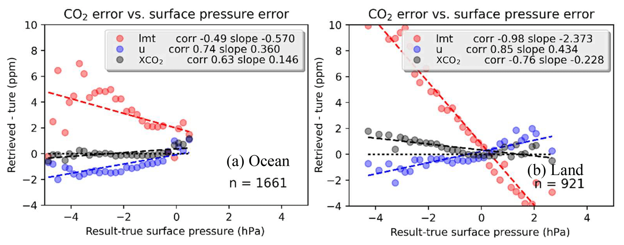
Figure 9Error in the lower partial column (LMT), upper partial column (U) and total column (XCO2) versus error in surface pressure (with 0.2 hPa bins) for ocean (a) and land (b). The OCO-2 v7 XCO2 bias versus dP is −0.3 for land and −0.08 for ocean.
The retrieval system must match the mean photon path length for the O2 A-band channel using retrieved parameters like surface pressure, albedo, water, temperature, aerosol pressure heights, and aerosol optical depths. Also note that the O2 volume mixing ratio (VMR) is fixed and not retrieved. Mean photon path length increases with higher albedo and aerosol optical depth (Palmer et al., 2001). Additionally, moving aerosols lower in the atmosphere increases mean photon path length, because light scattered by the aerosol travels farther, and a larger surface pressure will increase mean photon path length because the path length to the surface is longer. The retrieval system varies these parameters to match the observed radiances. Ideally, the three bands would have the same albedo and aerosol properties, so that getting the O2 A-band mean photon path length right will also get the mean photon path length in the CO2 bands. Real aerosol optical depths tend to be higher in the O2 A band than in the CO2 bands. However, the aerosol optical depth versus frequency is fixed for OCO-2. Therefore, as an example, using a too-thick aerosol in the O2 A band to compensate for a too-small surface pressure will not balance in the CO2 bands because the same too-small surface pressure will be offset by less aerosol. The relative strengths of the Jacobians for the four aerosol optical depths in the O2 A band versus CO2 bands are 1.5×, 3.3×, 7.2×, and 2.1×, respectively, indicating the dominance of the O2 A band concerning aerosol information.
As seen in Fig. 8b, for dP < −2 hPa, there is a negative bias in surface pressure (because we selected for this), negative biases in three of the four aerosol optical depths (green box, parameters 1, 4, and 10), positive bias in retrieved aerosol pressure (green box, parameters 2, 5, 8), and negative biases in the retrieved albedo (purple box, parameters 1, 3, 5). The error covariances show that (within this subset of observations) there are strong negative correlations between retrieved surface pressure error and errors in albedo and aerosol optical depth. There are also positive correlations between errors in aerosol optical depth and errors in albedo.
To trace the interferent errors to an error for XCO2, the effect of each bias on mean photon path length for the O2 A band and for weak and strong bands needs to be calculated, and then the mean photon path length error of the CO2 bands versus the O2 A band will give the error for XCO2. For example if the O2 A-band mean photon path length is perfect and the CO2 mean photon path length is 0.5 % too large relative to true, then the CO2 retrieved VMR will be 0.5 % too small. Since aerosols are compensating for errors in surface pressure, it is not ideal to fix their relationship versus frequency.
Figure 8d–f shows the bias patterns for these different groups. Comparing Fig. 7d, e, and f reveals patterns that could be used for screening: e.g., a low bias in Kahn 1 aerosol optical depth and low biases in all albedo means as well as high biases in all albedo slope indicate a negative surface pressure error, whereas a high bias in Kahn 1 aerosol pressure and width and a high bias in the strong band albedo slope indicate a positive surface pressure error. In real retrievals, a high albedo bias could not be distinguished from high true albedo; however, the pattern of biases observed in Fig. 8 could be used to identify low-quality retrievals (e.g., albedo higher than expected, aerosol OD larger than expected, and surface pressure lower than expected) and implies a bad result.
Table 9Predicted and actual errors and biases in raw and bias-corrected simulated data run with configuration (b) from Table 3. Similar to operational retrievals, bias-corrected XCO2 error is underestimated, whereas the CO2 partial column errors are overestimated. The XCO2 error underprediction results from overestimated error correlations of the partial columns.
It is interesting to note that the system appears to be able to compensate for and pass postprocessing quality screening, using albedo and aerosols, for low surface pressure biases down to −4 hPa but high surface pressure biases only up to +2 hPa.
4.3 Error correlation and effect of bias correction on errors
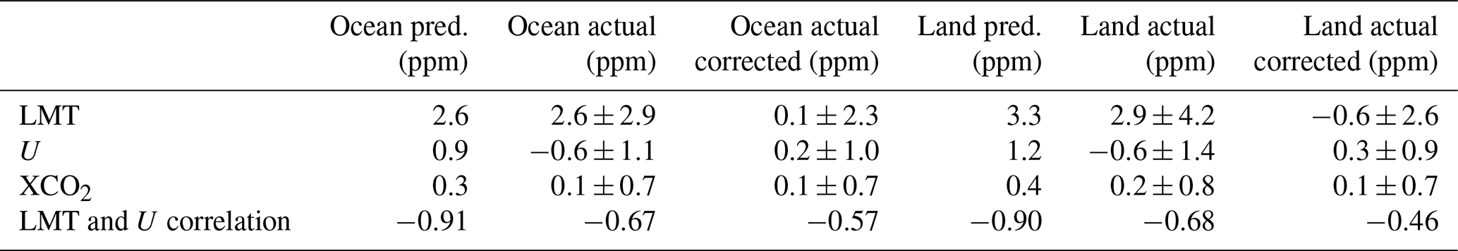
Another important question is the following: how does bias correction within the CO2 column affect errors, particularly the error correlations in XCO2 and the partial columns? Kulawik et al. (2017) found that the predicted error correlation between the LMT and U partial columns was −0.7 for land and −0.8 for ocean, whereas the actual error correlation versus aircraft was found to be +0.6 (with uncertainty in the correlation due to the fact that aircraft do not cover the full U partial column and effects of colocation error). Additionally, Kulawik et al. (2017) found that whereas the XCO2 predicted errors were underestimated by about a factor of 2, the LMT and U errors were overestimated by about a factor of 2. Weakening the LMT and U correlations would result in higher and more accurate error estimates for XCO2.
The errors for XCO2, LMT, and U for land and ocean for configuration (b) are summarized in Table 9. The bias correction for XCO2 (using only and dP) lowers the XCO2 bias from 0.2 to 0.1 ppm and the error from 0.8 to 0.7 ppm for land but has no impact on the ocean error or bias. The XCO2 error is underestimated by a factor of 2 for these simulation results, similarly to what was found with real data.
Similar to findings with real data, the XCO2 error in these simulations is underestimated, whereas the LMT and U errors are overestimated. However, the overestimate of the partial column errors are not as large as seen with real GOSAT data. The predicted error correlation is −0.91 for the LMT and U errors, whereas the actual error correlation is −0.5. Using Eq. (10c) from Kulawik et al. (2017), and the LMT and U errors in Table 9, we note two key results. First, the XCO2 predicted error is 0.37 ppm when the error correlation is −0.91. Second, the predicted XCO2 error is 0.64 (0.71) ppm for ocean (land) when the actual correlation is −0.57 (−0.46) for ocean (land). The second result is close to the actual error of 0.7 ppm. The estimate of +0.6 correlation from Kulawik et al. (2017) is probably wrong and could be due to unaccounted effects of colocation error on correlation estimates.
As seen in Sect. 3.1, nonlinearities from interferents affect both partial columns similarly. This would result in a positive error correlation (since the correlation is strongly negative and results in a less negative correlation than predicted) and explain the larger actual versus predicted XCO2 error. A high negative correlation is desirable for XCO2 because it asserts that, although there is uncertainty in the partitioning of LMT and U, the sum of the two has a smaller uncertainty.
The 15 orbits of simulated retrievals result in ∼10 000 land and ocean scenes for cloud-free runs, and 870 and 680 land and ocean cases for runs with clouds, after postprocessing quality screening. Prior to application of quality flags, described in Sect. 2.3, the errors are ∼10 ppm for land and ∼2 ppm for ocean. After quality flags and bias correction are applied, the errors are 0.7 ppm, with mean bias errors of 0.1 ppm for both land and ocean. There is a spatial pattern to the bias, which has similar characteristics to the spatial pattern of real OCO-2 biases, with a correlation length of ∼3∘, similar to the correlation length of 5–10∘ for OCO-2 (Kulawik et al., 2019a).
Comparing runs with and without measurement noise added to the radiances showed that the predicted measurement error is accurate. Comparing the retrieved results to the linear estimate using only the CO2 parameters (smoothing error) shows that the smoothing error is not greater than 0.5 ppm, but due to interferent error and nonlinearity this could not be validated more accurately with the tests used. A more accurate way to validate this would be to run tests with different priors (e.g., Kulawik et al., 2008), which was previously done (unpublished), finding that the smoothing errors are smaller than 0.2 ppm.
The linear estimate does not predict the nonlinear retrievals to better than 0.9 ppm (much worse when quality flags are not used), indicating this level of nonlinearity in the retrieval system. The interferent error is underpredicted by a factor of 4, based on the relationship of XCO2 error versus error for each retrieved interferent. The retrieved interferent error is twice as large as predicted for some parameters, and the correlation between the retrieved interferent error and XCO2 error is twice as large as predicted for some parameters. The larger correlation is likely due to the fact that CO2 Jacobian strength is correlated with many retrieved interferent values; a wrong interferent value will result in the wrong CO2 Jacobian strength, resulting in an error in CO2.
Two bias correction terms are explored: , the gradient of the retrieved CO2 profile relative to the prior state; and dP, the retrieved surface pressure minus the prior state. The bias correction could be explained by the following. (1) A loose CO2 constraint near the surface prefers changes near the surface versus changes elsewhere. (2) Since the CO2 Jacobian strength near the surface is stronger versus the Jacobian elsewhere in the profile, molecules incorrectly placed near surface are underestimated, because each molecule has too much of an effect on the observed radiance. (3) This results in an XCO2 column that is too low. This explanation would explain the positive bias correction factor seen in OCO-2 v7 land and v8 land and ocean but would not explain the negative correction factor seen in v7 ocean.
The theoretical basis for dP is complicated because so many other retrieval parameter errors are correlated to errors in dP. This makes sense from a fundamental radiative transfer perspective which ties together the surface and scattering properties with the amount of atmospheric column for any particular sounding. The retrieval system appears to use albedo and aerosols to compensate for errors in dP. In these simulated results the dP bias correction has a similar slope as seen in real OCO-2 data for land but not for ocean. The results with dP errors had marginally higher radiance residuals but not high enough to easily screen.
Similar to the findings in Kulawik et al. (2017), the XCO2 column error is much higher than predicted, whereas the lower and upper partial CO2 column errors, LMT and U, respectively, have errors lower than predicted. The underprediction of XCO2 error results because the retrieval system thinks the LMT and U partial column error correlation is −0.91. The actual correlation is −0.5 to −0.6 after bias correction, with the uncorrected results having both higher error and higher correlations in the partial columns. When the actual correlation is used to estimate XCO2 error, the predicted XCO2 error matches the actual error within 0.1 ppm. The reason why this correlation is off may be due to the fact that both partial column Jacobian strengths vary similarly with interferent errors, which are underpredicted in the linear estimates of errors, and would result in less negative correlation between the partial columns.
These results suggest a few possible strategies (a) isolating the primary interferent parameters via preretrievals of aerosols with surface pressure, CO2, and albedo fixed, followed by a full joint retrieval. This would allow clouds and aerosols to be approximately set without throwing the other retrieved parameters off. A similar technique was employed in the thermal infrared to mitigate cloud contamination (e.g., Eldering et al., 2008). A second tactic would be to perform retrievals beginning at many different initial states, selecting the result with the lowest radiance residual. This solution however is computationally expensive.
In summary, the simulated retrievals have many of the same attributes of real data, with the advantage of knowledge of the true state and ability to see what is going on under the hood. These simulation studies suggest attention should be given to nonlinearity, because the ability to estimate errors and make incremental improvements depends on the accuracy of the linear estimate, which has an accuracy of only about 0.9 ppm in these simulation studies.
Data are available at https://drive.google.com/file/d/1F_VfJOCfjlqVFLD3sY2zBjYbqPsrOVSW/view (Kulawik et al., 2019b).
SSK set the direction of the research, did the analysis, made figures, and was the primary manuscript writer. RRN and TET generated simulated OCO-2 true states, radiances, and retrievals. CO'D guided the work of the simulation system and advised on the analysis. All authors participated in the manuscript writing and editing.
The authors declare that they have no conflict of interest.
Plots were made using Matplotlib (Hunter, 2007).
This research has been supported by the NASA Roses (grant no. NMO710771/NNN13D771T, “Assessing Oco-2 Predicted Sensitivity And Errors”.
This paper was edited by Justus Notholt and reviewed by Sourish Basu and one anonymous referee.
Basu, S., Guerlet, S., Butz, A., Houweling, S., Hasekamp, O., Aben, I., Krummel, P., Steele, P., Langenfelds, R., Torn, M., Biraud, S., Stephens, B., Andrews, A., and Worthy, D.: Global CO2 fluxes estimated from GOSAT retrievals of total column CO2, Atmos. Chem. Phys., 13, 8695–8717, https://doi.org/10.5194/acp-13-8695-2013, 2013.
Chevallier, F., Palmer, P. I., Feng, L., Boesch, H., O'Dell, C. W., and Bousquet, P.: Toward robust and consistent regional CO2 fluxestimates from in situ and spaceborne measurements of atmospheric CO2, Geophys. Res. Lett., 41, 1065–1070, https://doi.org/10.1002/2013GL058772, 2014.
Connor, B. J., Boesch, H., Toon, G., Sen, B., Miller, C., and Crisp, D.: Orbiting Carbon Observatory: Inverse method and prospective error analysis, J. Geophys. Res., 113, D05305, https://doi.org/10.1029/2006JD008336, 2008.
Connor, B., Bösch, H., McDuffie, J., Taylor, T., Fu, D., Frankenberg, C., O'Dell, C., Payne, V. H., Gunson, M., Pollock, R., Hobbs, J., Oyafuso, F., and Jiang, Y.: Quantification of uncertainties in OCO-2 measurements of XCO2: simulations and linear error analysis, Atmos. Meas. Tech., 9, 5227–5238, https://doi.org/10.5194/amt-9-5227-2016, 2016.
Cressie, N., Wang, R., Smyth, M., and Miller, C. E.: Statistical bias and variance for the regularized inverse problem: Application to space based atmospheric CO2 retrievals, J. Geophys. Res.-Atmos., 121, 5526–5537, https://doi.org/10.1002/2015JD024353, 2016.
Crisp, D., Atlas, R. M., Breon, F.-M., Brown, L. R., Burrows, J. P., Ciais, P., Connor, B. J., Doney, S. C., Fung, I. Y., Jacob, D. J., Miller, C. E., O'Brien, D., Pawson, S., Randerson, J. T., Rayner, P., Salawitch, R. J., Sander, S. P., Sen, B., Stephens, G. L., Tans, P. P., Toon, G.C., Wennberg, P. O., Wofsy, S. C., Yung, Y. L., Kuang, Z., Chudasama, B., Sprague, G., Weiss, B., Pollock, R., Kenyon, D., and Schroll, S.: The Orbiting Carbon Observatory (OCO) Mission, Adv. Space Res., 34, 700–709, 2004.
Crisp, D., Fisher, B. M., O'Dell, C., Frankenberg, C., Basilio, R., Bösch, H., Brown, L. R., Castano, R., Connor, B., Deutscher, N. M., Eldering, A., Griffith, D., Gunson, M., Kuze, A., Mandrake, L., McDuffie, J., Messerschmidt, J., Miller, C. E., Morino, I., Natraj, V., Notholt, J., O'Brien, D. M., Oyafuso, F., Polonsky, I., Robinson, J., Salawitch, R., Sherlock, V., Smyth, M., Suto, H., Taylor, T. E., Thompson, D. R., Wennberg, P. O., Wunch, D., and Yung, Y. L.: The ACOS CO2 retrieval algorithm – Part II: Global data characterization, Atmos. Meas. Tech., 5, 687–707, https://doi.org/10.5194/amt-5-687-2012, 2012.
Crisp, D., Pollock, H. R., Rosenberg, R., Chapsky, L., Lee, R. A. M., Oyafuso, F. A., Frankenberg, C., O'Dell, C. W., Bruegge, C. J., Doran, G. B., Eldering, A., Fisher, B. M., Fu, D., Gunson, M. R., Mandrake, L., Osterman, G. B., Schwandner, F. M., Sun, K., Taylor, T. E., Wennberg, P. O., and Wunch, D.: The on-orbit performance of the Orbiting Carbon Observatory-2 (OCO-2) instrument and its radiometrically calibrated products, Atmos. Meas. Tech., 10, 59–81, https://doi.org/10.5194/amt-10-59-2017, 2017.
Eldering, A., O'Dell, C. W., Wennberg, P. O., Crisp, D., Gunson, M. R., Viatte, C., Avis, C., Braverman, A., Castano, R., Chang, A., Chapsky, L., Cheng, C., Connor, B., Dang, L., Doran, G., Fisher, B., Frankenberg, C., Fu, D., Granat, R., Hobbs, J., Lee, R. A. M., Mandrake, L., McDuffie, J., Miller, C. E., Myers, V., Natraj, V., O'Brien, D., Osterman, G. B., Oyafuso, F., Payne, V. H., Pollock, H. R., Polonsky, I., Roehl, C. M., Rosenberg, R., Schwandner, F., Smyth, M., Tang, V., Taylor, T. E., To, C., Wunch, D., and Yoshimizu, J.: The Orbiting Carbon Observatory-2: first 18 months of science data products, Atmos. Meas. Tech., 10, 549–563, https://doi.org/10.5194/amt-10-549-2017, 2017.
Eldering, A., Taylor, T. E., O'Dell, C. W., and Pavlick, R.: The OCO-3 mission: measurement objectives and expected performance based on 1 year of simulated data, Atmos. Meas. Tech., 12, 2341–2370, https://doi.org/10.5194/amt-12-2341-2019, 2019.
Eldering, A., Kulawik, S. S., Worden, J., Bowman, K., and Osterman, G.: Implementation of cloud retrievals for TES atmospheric retrievals: 2. Characterization of cloud top pressure and effective optical depth retrievals, J. Geophys. Res., 113, D16S37, https://doi.org/10.1029/2007JD008858, 2008.
Feng, L., Palmer, P. I., Parker, R. J., Deutscher, N. M., Feist, D. G., Kivi, R., Morino, I., and Sussmann, R.: Estimates of European uptake of CO2 inferred from GOSAT XCO2 retrievals: sensitivity to measurement bias inside and outside Europe, Atmos. Chem. Phys., 16, 1289–1302, https://doi.org/10.5194/acp-16-1289-2016, 2016.
Frankenberg, C., Kulawik, S. S., Wofsy, S. C., Chevallier, F., Daube, B., Kort, E. A., O'Dell, C., Olsen, E. T., and Osterman, G.: Using airborne HIAPER Pole-to-Pole Observations (HIPPO) to evaluate model and remote sensing estimates of atmospheric carbon dioxide, Atmos. Chem. Phys., 16, 7867–7878, https://doi.org/10.5194/acp-16-7867-2016, 2016.
Hobbs, J., Braverman, A., Cressie, N., Granat, R., and Gunson, M.: Simulation-Based Uncertainty Quantification for Estimating Atmospheric CO2 from Satellite Data, SIAM J. Uncert. Quant., 5, 956–985, 2017.
Hunter, J. D.: Matplotlib: A 2D graphics environment, Comput. Sci. Eng., 9, 90–95, 2007.
Kulawik, S. S., Bowman, K. W., Luo, M., Rodgers, C. D., and Jourdain, L.: Impact of nonlinearity on changing the a priori of trace gas profile estimates from the Tropospheric Emission Spectrometer (TES), Atmos. Chem. Phys., 8, 3081–3092, https://doi.org/10.5194/acp-8-3081-2008, 2008.
Kulawik, S. S., Crowell, S., Baker, D., Liu, J., McKain, K., Sweeney, C., Biraud, S. C., Wofsy, S., O'Dell, C. W., Wennberg, P. O.,Wunch, D., Roehl, C. M., Deutscher, N. M., Kiel, M., Griffith, D. W. T., Velazco, V. A., Notholt, J., Warneke, T., Petri, C., De Mazière, M., Sha, M. K., Sussmann, R., Rettinger, M., Pollard, D. F., Morino, I., Uchino, O., Hase, F., Feist, D. G., Roche, S., Strong, K., Kivi, R., Iraci, L., Shiomi, K., Dubey, M. K., Sepulveda, E., Rodriguez , O. E. G., Té, Y., Jeseck, P., Heikkinen, P., Dlugokencky, E. J., Gunson, M. R., Eldering, A., Crisp, D., Fisher, B., and Osterman, G. B.: Characterization of OCO-2 and ACOS-GOSAT biases and errors for CO2 flux estimates, Atmos. Meas. Tech., in review, 2019a.
Kulawik, S. S., O'Dell, C., Nelson, R. R., and Taylor, T. E.: Simulations for Kulawik et al., 2019, available at: https://drive.google.com/file/d/1F_VfJOCfjlqVFLD3sY2zBjYbqPsrOVSW/view, last access: 20 September 2019b.
Kulawik, S. S., O'Dell, C., Payne, V. H., Kuai, L., Worden, H. M., Biraud, S. C., Sweeney, C., Stephens, B., Iraci, L. T., Yates, E. L., and Tanaka, T.: Lower-tropospheric CO2 from near-infrared ACOS-GOSAT observations, Atmos. Chem. Phys., 17, 5407–5438, https://doi.org/10.5194/acp-17-5407-2017, 2017.
Mandrake, L., O'Dell, C., Wunch, D., Wennberg, P. O., Fisher, B., Osterman, G. B., and Eldering, A.: Lite Files, Warn Level and Bias Correction Determination, 2017.
Merrelli, A., Bennartz, R., O'Dell, C. W., and Taylor, T. E.: Estimating bias in the OCO-2 retrieval algorithm caused by 3-D radiation scattering from unresolved boundary layer clouds, Atmos. Meas. Tech., 8, 1641–1656, https://doi.org/10.5194/amt-8-1641-2015, 2015.
Nelson, R. R., O'Dell, C. W., Taylor, T. E., Mandrake, L., and Smyth, M.: The potential of clear-sky carbon dioxide satellite retrievals, Atmos. Meas. Tech., 9, 1671–1684, https://doi.org/10.5194/amt-9-1671-2016, 2016.
O'Brien, D. M., Polonsky, I., O'Dell, C., and Carheden, A.: The OCO simulator Orbiting Carbon Oservatory (OCO) Algorithm Theoretical Basis Document, Cooperative Institute for Research in the Atmosphere, Colorado State University, 2009-08-13, 2009.
O'Brien, D. M., Polonsky, I. N., Utembe, S. R., and Rayner, P. J.: Potential of a geostationary geoCARB mission to estimate surface emissions of CO2, CH4 and CO in a polluted urban environment: case study Shanghai, Atmos. Meas. Tech., 9, 4633–4654, https://doi.org/10.5194/amt-9-4633-2016, 2016.
O'Dell, C. W., Connor, B., Bösch, H., O'Brien, D., Frankenberg, C., Castano, R., Christi, M., Eldering, D., Fisher, B., Gunson, M., McDuffie, J., Miller, C. E., Natraj, V., Oyafuso, F., Polonsky, I., Smyth, M., Taylor, T., Toon, G. C., Wennberg, P. O., and Wunch, D.: The ACOS CO2 retrieval algorithm – Part 1: Description and validation against synthetic observations, Atmos. Meas. Tech., 5, 99–121, https://doi.org/10.5194/amt-5-99-2012, 2012.
O'Dell, C. W., Eldering, A., Wennberg, P. O., Crisp, D., Gunson, M. R., Fisher, B., Frankenberg, C., Kiel, M., Lindqvist, H., Mandrake, L., Merrelli, A., Natraj, V., Nelson, R. R., Osterman, G. B., Payne, V. H., Taylor, T. E., Wunch, D., Drouin, B. J., Oyafuso, F., Chang, A., McDuffie, J., Smyth, M., Baker, D. F., Basu, S., Chevallier, F., Crowell, S. M. R., Feng, L., Palmer, P. I., Dubey, M., García, O. E., Griffith, D. W. T., Hase, F., Iraci, L. T., Kivi, R., Morino, I., Notholt, J., Ohyama, H., Petri, C., Roehl, C. M., Sha, M. K., Strong, K., Sussmann, R., Te, Y., Uchino, O., and Velazco, V. A.: Improved retrievals of carbon dioxide from Orbiting Carbon Observatory-2 with the version 8 ACOS algorithm, Atmos. Meas. Tech., 11, 6539–6576, https://doi.org/10.5194/amt-11-6539-2018, 2018.
Palmer, P. I., Jacob, D.J., Chance, K., Martin, R. V., Spurr, R. D., Kurosu, T. P., Bey, I., Yantosca, Y., Fiore, A., and Li, Q.: Air mass factor formulation for spectroscopic measurements from satellites' Application to formaldehyde retrievals from the Global Ozone Monitoring Experiment, J. Geophys. Res., 106, 14539–14550, 2001.
Polonsky, I. N., O'Brien, D. M., Kumer, J. B., O'Dell, C. W., and the geoCARB Team: Performance of a geostationary mission, geoCARB, to measure CO2, CH4 and CO column-averaged concentrations, Atmos. Meas. Tech., 7, 959–981, https://doi.org/10.5194/amt-7-959-2014, 2014.
Rosenberg, R., Maxwell, S., Johnson, B. C., Chapsky, L., Lee, R. A. M., and Pollock, R.: Preflight Radiometric Calibration of Orbiting Carbon Observatory 2, IEEE T. Geosci. Remote, 55, 1994–2006, https://doi.org/10.1109/TGRS.2016.2634023, 2017.
Rodgers, C. D.: Inverse Methods for Atmospheric Sounding, World Scientifc, Singapore, 2000.
Taylor, T. E., O'Dell, C. W., Frankenberg, C., Partain, P. T., Cronk, H. Q., Savtchenko, A., Nelson, R. R., Rosenthal, E. J., Chang, A. Y., Fisher, B., Osterman, G. B., Pollock, R. H., Crisp, D., Eldering, A., and Gunson, M. R.: Orbiting Carbon Observatory-2 (OCO-2) cloud screening algorithms: validation against collocated MODIS and CALIOP data, Atmos. Meas. Tech., 9, 973–989, https://doi.org/10.5194/amt-9-973-2016, 2016.
Winker, D. M., Pelon, J., Coakley Jr., J. A., Ackerman, S. A., Charlson, R. J., Colarco, P. R., Flamant, P., Fu, Q., Hoff, R., Kittaka, C., Kubar, T. L., LeTreut, H., McCormick, M. P., Megie, G., Poole, L., Powell, K., Trepte, C., Vaughan, M. A., and Wielicki, B. A.: The CALIPSO mission: A global 3D view of aerosols and clouds, B. Am. Meteorol. Soc., 91, 1211–1229, https://doi.org/10.1175/2010BAMS3009.1, 2010.
Wunch, D., Wennberg, P. O., Toon, G. C., Connor, B. J., Fisher, B., Osterman, G. B., Frankenberg, C., Mandrake, L., O'Dell, C., Ahonen, P., Biraud, S. C., Castano, R., Cressie, N., Crisp, D., Deutscher, N. M., Eldering, A., Fisher, M. L., Griffith, D. W. T., Gunson, M., Heikkinen, P., Keppel-Aleks, G., Kyrö, E., Lindenmaier, R., Macatangay, R., Mendonca, J., Messerschmidt, J., Miller, C. E., Morino, I., Notholt, J., Oyafuso, F. A., Rettinger, M., Robinson, J., Roehl, C. M., Salawitch, R. J., Sherlock, V., Strong, K., Sussmann, R., Tanaka, T., Thompson, D. R., Uchino, O., Warneke, T., and Wofsy, S. C.: A method for evaluating bias in global measurements of CO2 total columns from space, Atmos. Chem. Phys., 11, 12317–12337, https://doi.org/10.5194/acp-11-12317-2011, 2011.
Wunch, D., Wennberg, P. O., Osterman, G., Fisher, B., Naylor, B., Roehl, C. M., O'Dell, C., Mandrake, L., Viatte, C., Kiel, M., Griffith, D. W. T., Deutscher, N. M., Velazco, V. A., Notholt, J., Warneke, T., Petri, C., De Maziere, M., Sha, M. K., Sussmann, R., Rettinger, M., Pollard, D., Robinson, J., Morino, I., Uchino, O., Hase, F., Blumenstock, T., Feist, D. G., Arnold, S. G., Strong, K., Mendonca, J., Kivi, R., Heikkinen, P., Iraci, L., Podolske, J., Hillyard, P. W., Kawakami, S., Dubey, M. K., Parker, H. A., Sepulveda, E., García, O. E., Te, Y., Jeseck, P., Gunson, M. R., Crisp, D., and Eldering, A.: Comparisons of the Orbiting Carbon Observatory-2 (OCO-2) XCO2 measurements with TCCON, Atmos. Meas. Tech., 10, 2209–2238, https://doi.org/10.5194/amt-10-2209-2017, 2017.