the Creative Commons Attribution 4.0 License.
the Creative Commons Attribution 4.0 License.
 | 05 Nov 2019
Retrieval of temperature from a multiple channel pure rotational Raman backscatter lidar using an optimal estimation method
Shayamila Mahagammulla Gamage
Giovanni Martucci
Alexander Haefele
We present a new method for retrieving temperature from pure rotational Raman (PRR) lidar measurements. Our optimal estimation method (OEM) used in this study uses the full physics of PRR scattering and does not require any assumption of the form for a calibration function nor does it require fitting of calibration factors over a large range of temperatures. The only calibration required is the estimation of the ratio of the lidar constants of the two PRR channels (coupling constant) that can be evaluated at a single or multiple height bins using a simple analytic expression. The uncertainty budget of our OEM retrieval includes both statistical and systematic uncertainties, including the uncertainty in the determination of the coupling constant on the temperature. We show that the error due to calibration can be reduced significantly using our method, in particular in the upper troposphere when calibration is only possible over a limited temperature range. Some other advantages of our OEM over the traditional Raman lidar temperature retrieval algorithm include not requiring correction or gluing to the raw lidar measurements, providing a cutoff height for the temperature retrievals that specifies the height to which the retrieved profile is independent of the a priori temperature profile, and the retrieval's vertical resolution as a function of height. The new method is tested on PRR temperature measurements from the MeteoSwiss RAman Lidar for Meteorological Observations system in clear and cloudy sky conditions, compared to temperature calculated using the traditional PRR calibration formulas, and validated with coincident radiosonde temperature measurements in clear and cloudy conditions during both daytime and nighttime.


High time and space resolution measurements of atmospheric temperature are necessary to improve our understanding of many atmospheric processes, both dynamical and chemical. Radiosounding is the most widely used method for temperature profiling in the troposphere and lower stratosphere and has the advantage of operation in most weather conditions, but is typically limited to two flights per day only at selected sites worldwide. Pure rotational Raman (PRR) lidars have excellent vertical and temporal resolution and can be combined with vibrational Raman channels to determine relative humidity (Mattis et al., 2002; Wang et al., 2011; Behrendt et al., 2002; Reichardt et al., 2012). Lidar temperature measurements can be assimilated with atmospheric models to improve weather forecasts, as recently demonstrated by Adam et al. (2016).
The traditional Raman lidar temperature retrieval method, introduced by Cooney (1972), uses the ratio of two PRR signals from the Stokes branch which have been corrected for saturation, background, and other instrumental effects as required. The PRR spectrum contains two branches: Stokes and anti-Stokes. Both branches have approximately the same intensity and they are positioned symmetrically in wavelength on either side of the excitation line. The traditional Raman lidar temperature retrieval algorithm requires the assumption of an analytic form of a lidar calibration function whose coefficients are usually determined with external measurements, such as radiosondes (Behrendt, 2005). The calibration function is an approximation of the relationship of the signal ratio and temperature and depends on two or more coefficients. Calibration errors exceeding 0.5 K can arise if the calibration data do not cover a sufficient temperature range (Behrendt, 2005).
Of primary importance is the calibration of the lidar returns to allow for absolute temperature measurements. In the traditional method, the ratio of the corrected photocounts is fit to a set of corresponding temperature data points usually obtained from radiosondes. Behrendt (2005) gives a comprehensive overview of the traditional rotational Raman lidar temperature calculation method. Over the years the traditional temperature method has been improved by advancements in the instrumentation capabilities and improvements to the estimation and calibration techniques. Below some examples of innovations in this area since the (Behrendt, 2005) review.
Radlach et al. (2008) and Weng et al. (2018) introduce changes to the their Raman lidar systems to improve the temperature measurements. Radlach et al. (2008) introduced a new high-resolution rotational Raman lidar system with a receiving system that uses multicavity interference filters in a sequential setup to improve the efficiency of the elastic and rotational Raman signal separation. Together with the filter adjustments they have made noontime temperature measurements with uncertainties less than 1 K up to 1 km for 1 min integration time. Weng et al. (2018) introduced a new PRR lidar system that effectively detects two isolated nitrogen molecule PRR line signals and elastic backscatter signals. With this new system, temperatures at any given time can be obtained without a calibration.
The accuracy of the traditional Raman temperature estimations is highly sensitive to the estimation of the calibration function and calibration coefficients. Zuev et al. (2017) has investigated the use of nonlinear calibration functions to improve the accuracy of the traditional Raman temperature estimation and relaxing the assumption of sampling two single PRR lines. The results showed the term expressed in a form of a quadratic function of log ratio of the PRR measurements as best for practical use. He et al. (2018) proposed a new calibration method for PRR lidar temperature profiling based on the different temperature sensitivities of Stokes and anti‐Stokes PRR lines. They reconstruct the expression of the differential backscatter cross section according to the temperature dependencies of each component and form both a temperature factor and a calibration factor in the intensity ratio. This new method reduces the temperature error by 50 % compared with commonly used calibration methods in conditions of low signal‐to‐noise ratio (SNR).
Yan et al. (2019) has proposed an iterative method for determining Raman temperature. Their method allows independent alternating solutions to the high- and low-quantum-number PRRs separately, where high-quantum-number PRR lidar returns are used to solve for the channel constant, while low-quantum-number PRR returns with higher SNR are used for retrieving temperature profiles in an iterative fashion. Their results showed that the effective temperature retrieval height for their system improved from 17 to 25 km.
The application of the optimal estimation method (OEM) for temperature retrievals using pure rotational Raman (PRR) lidar measurements has several advantages over the traditional method, including the ability to find temperature without assuming an analytic form of the temperature or count ratio relation. Our OEM retrieval does not use the ratio of the counts. Rather we use a forward model which includes complete physics to describe the raw count profiles. For calibration, the ratio of the lidar constants, here referred to as coupling constant, needs to be determined. The coupling constant can in principle be estimated at a single point, such as a nearby flux tower or surface measurement. Our OEM retrieval has other important benefits over the traditional method as it can directly retrieve ancillary parameters (in addition) to temperature, such as geometrical overlap, particle extinction, and the lidar constant. Our OEM is also capable of providing a full uncertainty budget, including both random and systematic uncertainties on a profile-by-profile basis, including the systematic uncertainty introduced in the retrieved temperature by the estimation of the coupling constant. The OEM is an inverse method and is a standard tool in the retrieval of geophysical parameters from passive atmospheric remote sensing instruments. Recent studies including Povey et al. (2014); Sica and Haefele (2015, 2016), and Farhani et al. (2019) have shown that OEM can be used to retrieve atmospheric aerosol, water vapour mixing ratio, middle and upper atmospheric temperature, and ozone using lidar measurements.
In Sect. 2 a brief description of the instrument and the measurements used in this study is presented. Section 3 presents the development of the PRR lidar equation.
The development of a forward model for application of the OEM to PRR temperature retrieval is given in Sect. 4. The OEM-retrieved temperature results from the PRR measurements for different atmospheric conditions are shown in Sect. 5. A discussion of these results is presented in Sect. 6, followed by conclusions.
PRR measurements from the RAman Lidar for Meteorological Observations (RALMO), located in Payerne, Switzerland (46∘48′ N, 6∘56′ E), are used for the OEM temperature profiling. RALMO is a fully automated lidar built at the École Polytechnique Fédérale de Lausanne and operated by MeteoSwiss (Dinoev et al., 2013). It is dedicated to operational meteorology, validating models and satellite measurements, and climate studies. RALMO has been operating nearly continuously since 2008, with an average data availability of 50 %. Data gaps are due to rain and low clouds (approximately 30 % of the time), maintenance (1–2 d per month), and other occasional technical problems. RALMO consists of a frequency-tripled Q-switched Nd:YAG laser of 354.7 nm producing up to 400 mJ of emission energy at a 30 Hz repetition rate. The pulse duration is 8 ns. The laser is operated at 300 mJ of energy per pulse to extend the lifetime of the flash lamps from 20 to approximately 60 million shots. The RALMO receiver uses four parabolic mirrors, each with 1 m focal length and 30 cm diameter, and it is fiber coupled to a two-stage grating polychromator. The data acquisition system consists of photomultipliers and analog or photon-counting transient recorders from Licel. The system obtains a measurement by adding together 1800 laser shots (every minute) at a vertical resolution of 3.75 m. For a detailed description of the lidar and a detailed validation of the temperature measurements, the reader is referred to Dinoev et al. (2013).
The returns of the Raman-shifted backscatter arising from rotational energy state transitions of nitrogen and oxygen molecules due to the excitation at the laser wavelength at 354.7 nm are detected in analog or photon-counting mode. The high-quantum-number channel (JH) of RALMO is assigned to the backscattered signals from the energy exchange that occurs in the high-quantum-number states for both the Stokes (355.77–356.37 nm) and anti-Stokes (353.07–353.67 nm) branches. The low-quantum-number channel (JL) is assigned to the signals from the energy exchange occurring in the low-quantum-number states in the Stokes (355.17–355.76 nm) and anti-Stokes (353.67–354.25 nm) branches.
The backscattered PRR signal is given by the Raman lidar equation:
where the true backscattered PRR signal, NRR,t, is a function of height z, CRR is the lidar constant, n(z) is the number density of the air molecules, O(z) is the geometrical overlap, ηi is the volume mixing ratio of nitrogen and oxygen, Γatm(z) is the atmospheric transmission, is the attenuated differential backscatter cross section for each RR (rotational Raman) line Ji, and BRR(z) is the background of the measured signal. For different lidar systems the background can either be a constant or vary with height. Since air below 80 km is a constant mixture of oxygen and nitrogen, ηi is a constant. The lidar constant CRR depends on the number of transmitted photons, detector efficiency, and the area of the telescope. The attenuated differential backscatter cross section for Stokes and anti-Stokes line pairs of equal quantum number of the PRR spectrum is expressed as (Penney et al., 1974):
where for the Stokes branch
and for the anti-Stokes branch
τ+(Ji) and τ−(Ji) are the transmissions of the receiver for the Stokes and anti-Stokes lines Ji, respectively. gi(J) is the statistical weighting factor, which depends on the nuclear spin Ii for each atmospheric constituent, h is Planck's constant, c is the velocity of light, k is Boltzmann's constant, B0,i is the ground-state rotational constant, v0 is the frequency of the incident light, and ζi is the anisotropy of the molecular polarizability. The rotational energy Erot,i(J) for each Stokes and anti-Stokes branch is estimated based on the assumption of a homonuclear diatomic molecule in the quantum state J for nitrogen and oxygen molecules with no electronic momentum coupled to the scattering (Behrendt, 2005).
The response of the photomultiplier tubes operated in the photon-counting mode can become nonlinear at high count rates. In the case of RALMO, the true and observed counts are related by the equation for non-paralyzed systems:
where γ is the counting system dead time.
4.1 Brief review of the optimal estimation method
The OEM is an inverse method that uses the measurements y to estimate the state (retrieval) variables x of a system via a forward model. The forward model F contains all the atmospheric and instrumental physics that describe the measurements. The forward model can include model parameters b, which are assumed and not retrieved, and their effect on the retrieved quantity uncertainties can be calculated.
The measurements are related to the forward model by
where ϵ represents measurement noise. Under the assumption that all parameters have Gaussian probability density functions Bayes’ theorem can be applied to determine the cost function,
where xa is the a priori of the retrieval parameters, Sy is the measurement covariance, which describes the random measurement uncertainty, and Sa is the a priori covariance. The cost function measures the goodness of fit for a solution, and for good models the cost is on the order of unity. For nonlinear forward models, the Marquardt–Levenberg method can be used iteratively to minimize the cost of the retrieval (see Sect. 5.7 in Rodgers, 2000, for details).
The uncertainty budget is determined from the measurement and model parameter covariance matrices (Rodgers, 2000). The total error covariance, Stotal, is
where Sm is the retrieval covariance due to measurement noise and SF is the retrieval covariance due to the forward model parameter uncertainty. The retrieval covariance due to measurement noise, Sm, is
where G is the gain matrix, which is the sensitivity of the retrieval to the measurements. The retrieval covariance due to the forward model parameters, SF, is
where Kb and Sb are the forward model parameter Jacobian and covariance matrices, respectively. The model parameter Jacobians, Kb, can be estimated analytically or numerically for each model parameter. To construct Sb we require the uncertainties in the model parameters. We recommend Rodgers (2000) for more details of the OEM.
4.2 The forward model for a PRR lidar
The forward model describes the measurement as a function of both the state of the atmosphere and instrumental parameters. The core of our forward model is the lidar equation as presented in Sect. 3. It is called four times to generate the measurements corresponding to high and low quantum numbers, i.e. JH and JL, with photon-counting and analog detection. Analog detection is assumed to be linear.
The pressure, P(z), and temperature, T(z), can be taken from either a radiosonde measurement or an atmospheric model. The background noise, BRR, is in general a function of height, z, but is constant with height for RALMO. Unlike all the other existing forward models for lidar except Povey et al. (2012) (which was designed specifically to determine overlap), we retrieve O(z) the geometrical overlap function in addition to temperature. The overlap functions of JH and JL channels were assumed to be the same (Dinoev et al., 2010).
The atmospheric transmission, Γatm(z) in Eq. (1), includes both molecular and particle scattering.
where αmol is the molecular extinction coefficient and αpar is the particle extinction coefficient. The molecular extinction can be expressed using the Rayleigh cross section σRay and air density nair as
where σRay is calculated using the expressions given by Nicolet (1984).
For each channel the subscript RR is replaced by JL and JH, the high- and low-quantum-number PRR channels. Then CRR, BRR, and Ji have different values.
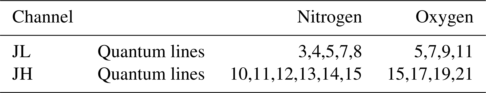
RALMO detects multiple Stokes and anti-Stokes lines from both nitrogen and oxygen in a PRR spectrum. Therefore, to determine the attenuated backscatter cross-section in the forward model, we require knowledge of the exact number of quantum states detected by each RALMO PRR channel. From the JH and JL channel characteristics we can calculate the range of frequency shifts for each channel relative to the elastic wavelength 354.7 nm. Then using the equations given by Herzberg (2013) we can determine the quantum numbers Ji for both nitrogen and oxygen molecules. This calculation process is repeated to determine the Ji numbers for the JL channel of the RALMO. A summary of the findings is given in Table 1.
Table 1The respective quantum lines from both nitrogen and oxygen in a PRR spectrum detected by the RALMO temperature polychromator. Note the given quantum lines are valid for both the Stokes and anti-Stokes branches.
In order to establish absolute calibration, we define the coupling constant R as the ratio of the lidar constants CJL and CJH,
and use the substitution CJH=RCJL. The coupling constant is height independent and can be determined with no assumptions at, if desired, a single altitude using the following equation derived from Eq. (1).
The differential cross section terms are determined by applying temperature from a coincident reference temperature, typically from a radiosonde. For a well designed lidar system the coupling constant should be stable over weeks. Unlike the fitting of an analytic calibration function to the data as in the traditional method, R can be estimated at a specific height or range of heights, which can be over a narrow range of temperature without introducing extrapolation errors. We extensively tested this assertion using both synthetic and real measurements. The results show that the estimation of R is indeed height independent. The value of R is only affected by the measurement noise. Hence, we recommend using a range of heights or a specific height where the photocounts have a high signal-to-noise ratio.
Using R in the forward model allows us to retrieve only one lidar constant, while constraining the two channels to vary so as to satisfy Eq. (13). We will see in the next section that any variations or uncertainty in the determination of R introduces an uncertainty on the order of 0.2 K to the retrieved temperature profile.
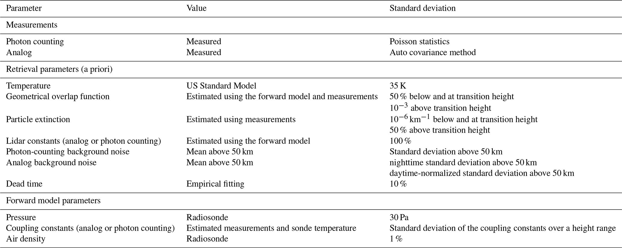
The retrieval parameters (Table 2) in our OEM algorithm are temperature, background signals (including photomultiplier shot noise, sky background, and offset for analog channels), the lidar constants, dead times of the photon-counting systems, geometrical overlap, and particle extinction as a function of height. In OEM we can retrieve parameters on a height grid where the resolution can be the same or different than the vertical resolution of the height grid that the measurements obtained. If the retrieval grid is coarser than the measurement grid, we use linear interpolation on retrieved quantities when they are required in the forward model.
Table 2Values and associated uncertainties for the OEM retrieval and forward model parameters.
4.3 Implementation of the RR temperature retrieval
The OEM solver in the Qpack software package is used for our retrieval (Eriksson et al., 2005). The solver requires the following as inputs: the measurements from each lidar channel and their covariances, a priori values for the retrieval parameters and their covariances, model (b) parameters and their covariances, and the Jacobians of the forward model.
The lidar measurements from the photon-counting channels follow Poisson counting statistics in the range where the counts are linear. Thus, the measurement variance Sy is equal to the number of photons in each height bin, assuming no correlation between the height bins (that is, the off-diagonal terms in the Sy matrix are zero). The autocorrelation function method of Lenschow et al. (2000) is used to estimate the measurement covariance of the analog and photon-counting measurements in the nonlinear region. For both analog and photon-counting channels, the a priori backgrounds and their variances are taken as the mean and the variance of the measurements above 50 km height.
The U.S. Standard Atmosphere (NASA, 1976) model temperature profile is normalized to the surface temperature from the coincident sonde temperature and then used as the a priori temperature profile in our retrievals. Due to the high variability in the temperature, a standard deviation of 35 K for all heights is used to specify the covariance matrix for a priori values. Other choices of a priori temperature profile are possible but as an operational fully automated lidar system RALMO retrievals must be performed automatically every 30 min, so the choice of the U.S. Standard Atmosphere with this covariance simplifies this procedure. As discussed in Eriksson et al. (2005), the elements of the retrieval and model parameters are often correlated, and some of the covariance matrices should have off-diagonal elements. Off-diagonal elements are parameterized with the correlation length and an appropriate analytical function describing the decay of the correlation. For this study, we used a tent function with a 1 km correlation length for temperature retrievals (Eriksson et al., 2005).
Molecular and particle extinction terms occur in the atmospheric transmission term of Eq. (11). An a priori particle extinction profile is estimated based on the following expression:
where LR is the lidar ratio and βpar is the particle backscatter coefficient. βpar is related to the backscatter ratio ℜβ as (Whiteman, 2003):
The backscatter ratio ℜβ is estimated using the RALMO PRR and elastic measurements. Bucholtz (1995) gives a method for calculating βmol using pressure, temperature, and Rayleigh cross sections. The Rayleigh extinction cross sections required for βmol estimation are computed using the formula of Nicolet (1984). Calculated Rayleigh extinction cross sections are also used to estimate the air density profile used as a b parameter in the forward model, assuming an uncertainty of 1 % for the standard deviation.
The lidar ratio LR is chosen based on the ℜβ values for the given measurements. Typically ℜβ values inside clouds are greater than 2. Thus, for this study the height at which ℜβ is first equal to 2 is considered the height of the cloud base or the height of an aerosol layer (cloud or aerosol layer base height). The cloud or aerosol layer base height is later used to determine the transition height that constrains the range of the geometrical overlap and the particle extinction retrievals. In cloud-free sky conditions that we will refer to as clear sky conditions from here on (that is if ℜβ does not exceed 2), LR is assumed to be 80 sr inside the boundary layer and 50 sr elsewhere. In cloudy conditions, LR is assumed to be 20 sr within the clouds present below 6 km. If the cloud is above 6 km, LR is assumed to be 15 sr within the cloud. These choices for lidar ratios are taken from Ansmann et al. (1992a) and Pappalardo et al. (2004). Accurate LR is not crucial, as it is used to estimate an a priori particle extinction profile. However, we can calculate a LR profile using the OEM-retrieved αpar and compare it with the initially chosen LR values to evaluate how good a choice of the initial value is.
The effect of geometrical overlap and particle extinction on the signals is coupled and hence retrieving both parameters simultaneously is not possible unless at least one of the effects is highly constrained. The particle extinction is indefinitely measured using the backscatter ratio outside clouds, and overlap is well known above the height of full overlap, i.e. above 6 km (Dinoev et al., 2010). We use this knowledge to define a transition height, in clear skies 6 km or at the cloud base height, whatever is lower. Below this height overlap is retrieved and above this height particle extinction is retrieved. The a priori overlap function is estimated from measurements in clear-sky conditions. A 50 % standard deviation is used for geometrical overlap below the transition height and a constant standard deviation of 10−3 is used above this height, constraining the geometrical overlap to the a priori values above the transition height. For particle extinction, a standard deviation of is used below the transition height to constrain the retrieval, then a 50 % standard deviation is used above this height, allowing the OEM to retrieve exclusively the particle extinction. The a priori covariance matrices for both particle extinction and geometrical overlap are determined using a tent function with a 100 m correlation length.
The a priori lidar constants for the JL analog and JL photon-counting channels are estimated by fitting the measurements generated using the sonde temperature and pressure used in the forward model to the PRR measurements. For analog measurements, the fitting range is between 1.5 to 2 km height. For photon-counting measurements with clear conditions or cloud/aerosol presence above 8 km, 6 to 8 km is used as the fitting range to ensure the photocounts are linear. If the photon-counting measurements contain cloud or aerosols in the geometrical overlap region, a fitting range below this is used, typically 3.5–4 km height. The fitting uncertainty for each analog and photon-counting lidar constants is used as the variance of the a priori lidar constant.
The a priori dead times for the two photon-counting systems are considered to be 3.8 ns, consistent with estimations from previous studies for RALMO and with values specified by the manufacturer (Sica and Haefele, 2015, 2016; Dinoev et al., 2010). The uncertainty in the dead time is taken as 10 %. Coincident radiosonde pressure profiles are used assuming a 10 % standard deviation. The coupling constants for analog (Ra) and photon-counting (R) channels are estimated by fitting the ratio of PRR measurements with the ratio of the differential cross section (Eq. 14). The coupling constants are estimated using the same fitting range as the lidar constants. Table 2 gives a summary of the parameters and associated uncertainties in the retrieval and model parameters used in the forward model.
We present four different measurement situations which demonstrate the robust nature of our OEM temperature retrieval. Details of each case study are given in Table 3. The RALMO measurements used in the retrievals are added in time over 30 min and to 15 m in height. Analog measurements are used from the surface to 6 km height, while photon-counting measurements are used from 4 to 28 km. The retrieval grid has a vertical resolution of 60 m at all heights. For all the cases given in Table 3 we used radiosonde measurements that coincide within 1 h of the lidar measurements for comparison purposes to estimate the required a priori information and to determine the forward model b parameters (Table 2).
Table 3Details of the four cases in clear and cloudy sky conditions we present to demonstrate the flexibility of our OEM temperature retrieval.
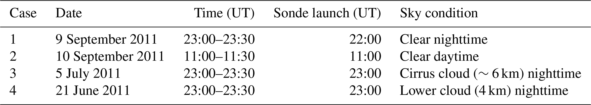
The traditional temperature profiles that will be shown later in this section are calculated using count profiles consisting of glued analog and photon-counting measurements, which are corrected for nonlinearity and background before processing. The vertical resolution of the traditional temperature profiles is 30 m at the lowest heights, increasing to 400 m by the upper heights to decrease the magnitude of the statistical uncertainty. A calibration function linear in 1∕T is used and the two coefficients have been determined with radiosonde data using the altitude range from the surface to 10 km. Hence, for this comparison the (traditional method) temperature profile is smoother than the OEM-retrieved temperature profile. The change in vertical resolution is based on the random uncertainty in the temperature profile at each height. The vertical resolution is decreased until the temperature uncertainty becomes less than a threshold value, set here as 1 K.
5.1 Case 1: nighttime with clear conditions
Figure 1 shows the RALMO 30 min coadded count measurements in the four PRR channels for case 1 given in Table 3. The analog signal is linear over its entire range. The photon-counting measurements are affected by nonlinearity below about 9 km for the JL channel (6 km for JH) by about 0.5 % (count rates of about 1 MHz) and as much as 10 % for the JL photon counts around 4 km altitude (Eq. 5).
Figure 2 shows the residuals, which are defined as the difference between the forward model and the measurements. For a good retrieval with cost on the order of unity, the residuals (blue curve) should be on the order of the standard deviation of the measurement noise (red curve), and indeed this is the case, hence the forward model is not over-fitting the measurements (e.g. cost much less than unity).

Figure 1Count rate for 30 min of coadded RALMO measurements from 23:00 UT on 9 September 2011, a clear night; (a) Photon-counting channels (blue curve, JL; red curve, JH); (b) Analog channels.
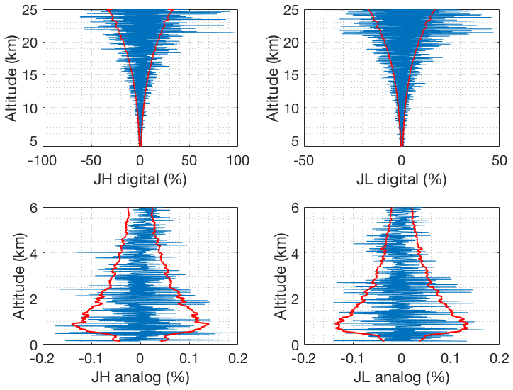
Figure 2Difference between the forward model and clear nighttime RALMO measurements on 9 September 2011 for the four signals (blue). The red curves show the standard deviation of the measurements noise.
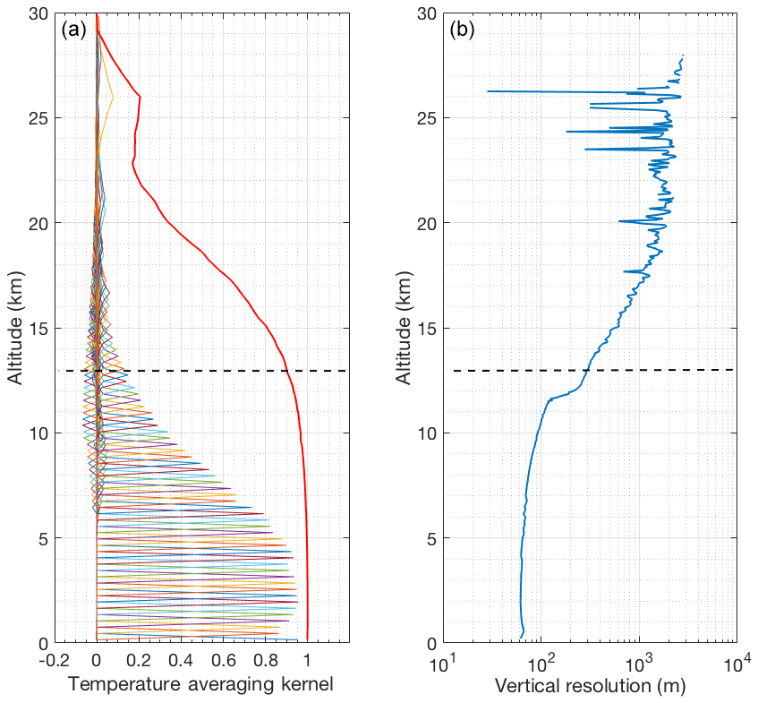
The averaging kernels of temperature and the vertical resolution of the retrievals are shown in Fig. 3. The area of the averaging kernels is defined as the response function of the retrievals and is close to 1.0 below 24 km, meaning that a contribution of the a priori temperature profile to the retrieved temperature is negligible (Rodgers, 2000). With decreasing signal-to-noise ratio the measurement response quickly decreases above about 27 km (Fig. 3). The full width at half maximum of the averaging kernels is the retrieval’s vertical resolution (Fig. 3b). The vertical resolution of the retrieval is smaller than the resolution of the retrieval grid above about 10 km. We consider the height at which response function decreases to 0.9 as the cutoff height for the OEM retrievals as at this level the contribution of the a priori temperature profile is about 10 %.
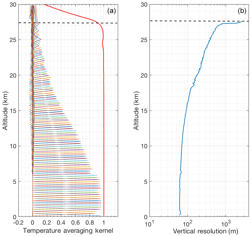
Figure 3Averaging kernels (a) and vertical resolution (b) for temperature retrievals from the clear nighttime RALMO measurements on 9 September 2011. The area of the averaging kernels at each height, the response function, is the solid red line. The horizontal dashed line shows the height below which the retrieval is due primarily to the measurement and not the a priori temperature profile. For clarity averaging kernels for every fifth height bin of the retrieval grid are shown.
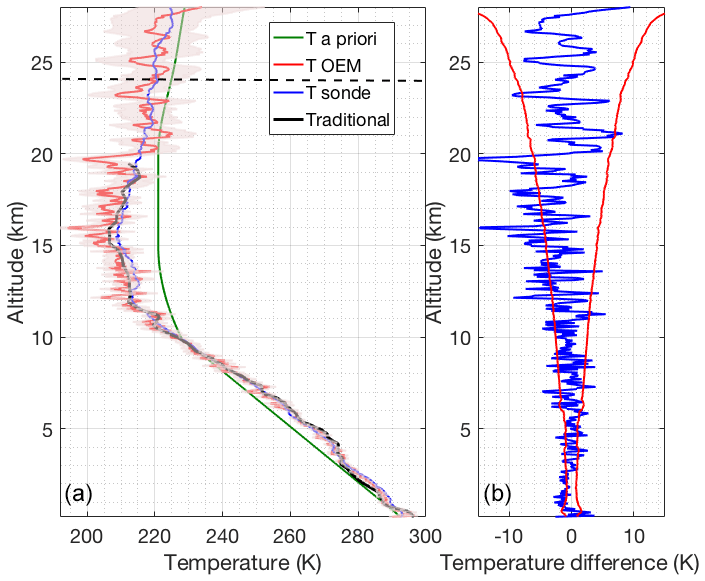
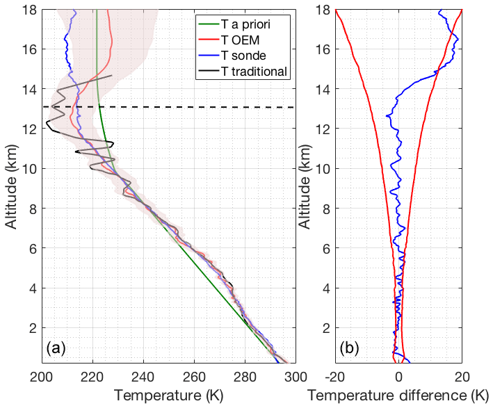
Figure 4(a) Retrieved temperature profile and the statistical uncertainty (red curve and shaded area) using the OEM from the clear nighttime RALMO measurements on 9 September 2011. The blue curve is the radiosonde measurement. The sonde was launched at 22:00 UT. The green curve is the a priori temperature profile used by the OEM. The black curve shows the temperature retrieved using the traditional analysis method from glued analog and photon-counting signals. The horizontal dashed line shows the height below which the retrieval is due primarily to the measurement and not the a priori temperature profile. (b) The blue curve shows the temperature difference between OEM-retrieved temperature and the sonde temperature. The red curves in the figure show the statistical uncertainty in the OEM temperature.
Figure 4 shows a comparison of the OEM-retrieved temperature profile with coincident sonde temperature and temperature obtained using the traditional method. The traditional method profile from the RALMO glued (photon-counting and analog) measurements provided by MeteoSwiss has a vertical resolution of 30 m below 12.5 km and 400 m above this height, and is interpolated to the same retrieval grid as the OEM and shown in black. The change in vertical resolution and the cutoff height of the traditional temperature retrieval are based on temperature uncertainty thresholds. As shown in Fig. 4b, the temperature difference between OEM-retrieved and sonde temperature (blue curve) fits inside the statistical uncertainty in the OEM-retrieved temperature. Temperatures from the traditional method follow the same trend as the sonde and the OEM-retrieved temperatures.
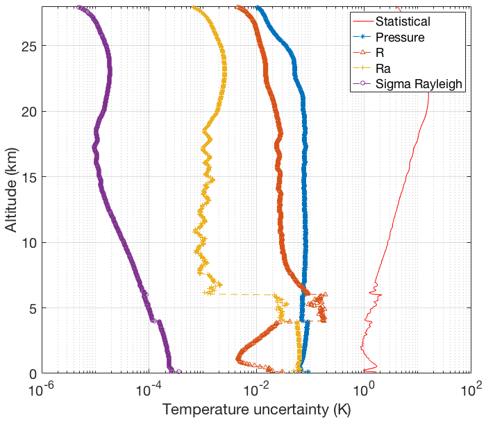
The OEM provides a complete uncertainty budget in both random and systematic uncertainties (Fig. 5). Uncertainties due to the Rayleigh cross section are on the order of 0.01 mK. Pressure accounts for up to 0.1 K below 10 km and up to 0.7 K up to 25 km and is a non-negligible source of uncertainty in the stratospheric part of the retrieval. Note that this error could be reduced by choosing a better pressure profile. The uncertainty due to the analog coupling constant Ra is on the order of 0.07 K up to 4 km and the uncertainty due to photon-counting coupling constant R is 0.15 K in the 4–7 km height range and less than 0.1 K everywhere else. The largest contribution to the temperature uncertainty is from measurement noise, which increases with height.
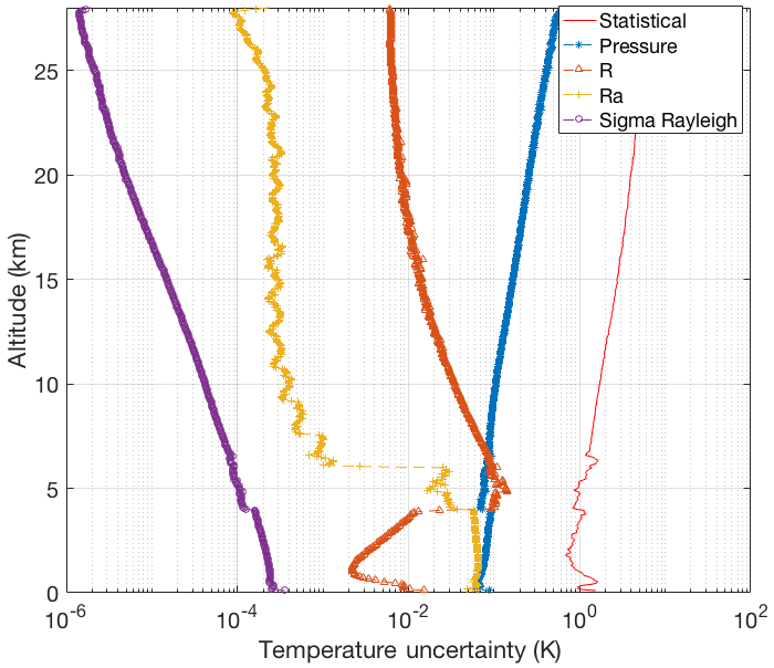
Figure 5Random uncertainties (red curve) and systematic uncertainties due to the forward model parameters for the temperature retrievals from the clear nighttime RALMO measurements on 9 September 2011. The systematic uncertainties included are Rayleigh-scatter cross section (purple dot-dashed curve), R photon-counting coupling constant (dashed orange curve with triangles), Ra analog coupling constant (dashed yellow curve with crosses), and pressure (dashed blue curve with dots).
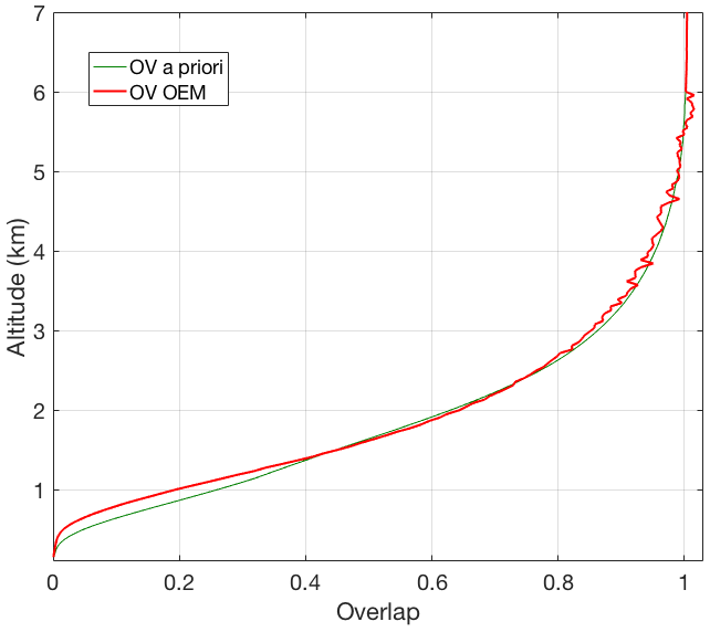
Figure 6Retrieved geometrical overlap function (red curve) from the clear nighttime RALMO measurements on 9 September 2011 compared to the a priori geometrical overlap function (green curve).
Figure 6 shows the OEM-retrieved geometrical overlap function for the RALMO PRR channels. It illustrates that the overlap retrieval is constrained to be equal to 1 above the transition height (6 km), above which the extinction coefficient is retrieved (see Sect. 4.3).
5.2 Case 2: daytime with clear conditions
The retrieval setup for the second case study, which is a daytime measurement (Table 3), is identical to the one used for nighttime. The major difference between daytime and nighttime retrievals is the large solar background in the measurements, which is evident in the measurements of the photon-counting PRR channels (Fig. 7).
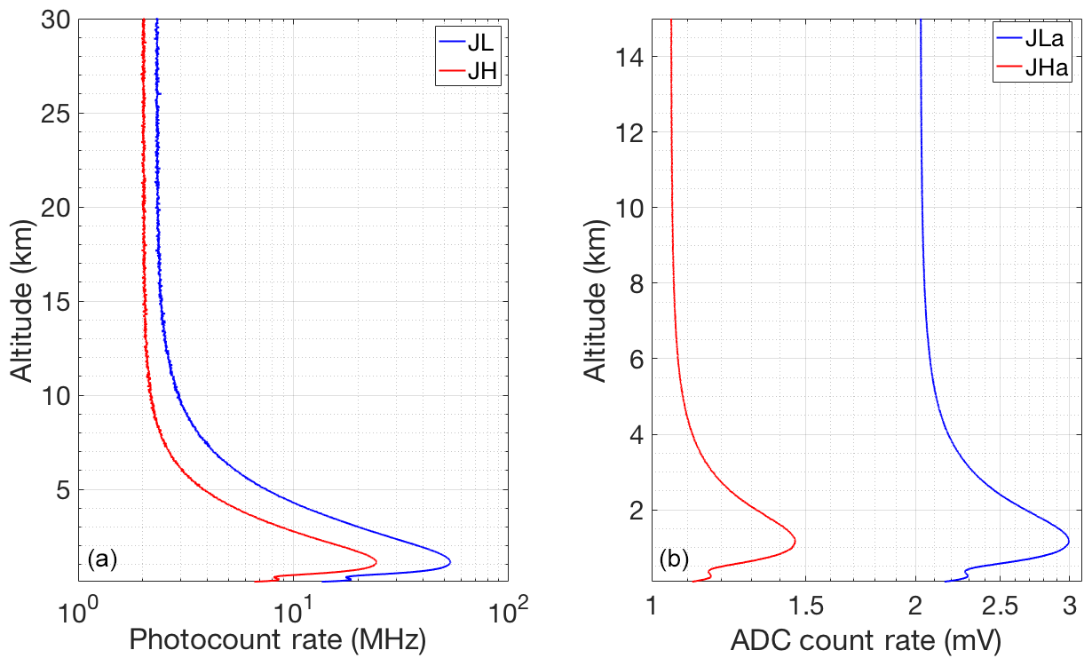
Figure 7Count rate for 30 min of clear coadded RALMO measurements from 11:00 UT on 10 September 2011; (a) Photon-counting channels (blue curve, JL; red curve, JH); (b) Analog channels.
The residuals are unbiased and fall within the limits of the measurement standard deviation (Fig. 8). This result confirms the capability of our forward model in daytime conditions. As shown in Fig. 9, the vertical resolution (Fig. 9b) is the same as the retrieval grid below 13 km where response function (Fig. 9a) is equal to 0.9. The vertical resolution starts to deviate from the retrieval grid as the response function decreases and the background starts to dominate the photon-counting channels.
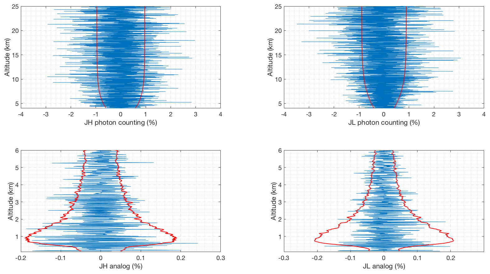
Figure 8Difference between the forward model and the clear daytime RALMO measurements on 10 September 2011 for the four signals (blue). The red curves show the standard deviation of the measurements.
Similar to the clear nighttime case, the OEM-retrieved temperature agrees with the sonde temperature within the statistical uncertainty (Fig. 10). It is also evident for this specific case study that the temperature from the traditional method deviates from the sonde temperature more than the OEM-retrieved temperature. This difference compared to the traditional method is due to the fact that the OEM adapts the vertical resolution in an optimal way as a function of height, while the traditional method is constrained by the filter employed to a specific signal-to-noise ratio of the measurements from both channels.
The analog coupling constant Ra uncertainty in the temperature from the daytime measurements is also on the order of 0.07 K and the uncertainty due to photon-counting coupling constant R is less than 0.2 K for all heights.
The retrieved geometrical overlap function for the clear daytime case (not shown) agrees with the geometrical overlap retrieved for the nighttime case within 10 % statistical uncertainty.
5.3 Case 3: nighttime with cirrus cloud
The third case (details are given in Table 3) features a cirrus cloud at 6 km height (Fig. 12).
The retrieval setup is identical to the previous cases, as the cloud base is above the height of full geometrical overlap of the transmitter and receiver. The a priori profile of the particle extinction coefficient is derived from the backscatter ratio assuming a lidar ratio of 15 sr.
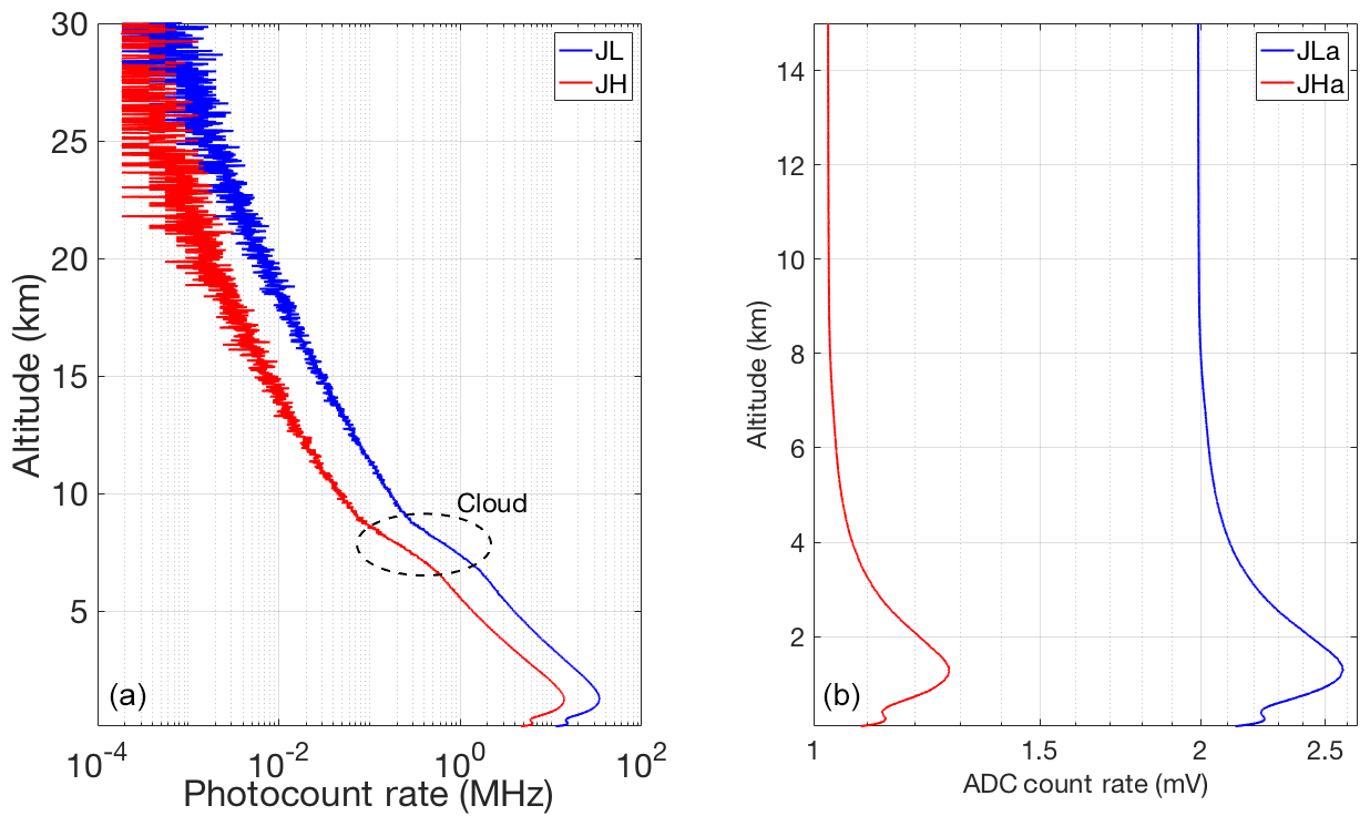
Figure 12Count rate for 30 min of coadded RALMO measurements from 23:00 UT on 5 July 2011; (a) Photon-counting channels (blue curve, JL; red curve, JH); (b) Analog channels.
The residuals (Fig. 13) are unbiased and fall within the square root of the measurement variance. This is also true for the altitude range of the cirrus cloud demonstrating that the particle extinction coefficient was determined correctly. The response function (Fig. 14a) decreases to the 0.9 cutoff value at about 23.5 km, clearly lower than the clear-sky nighttime case because of the attenuation of the cirrus cloud. Similar to the two previous cases, the OEM-retrieved temperature agrees with the sonde temperature within the statistical uncertainty in the OEM-retrieved temperature (Fig. 15).
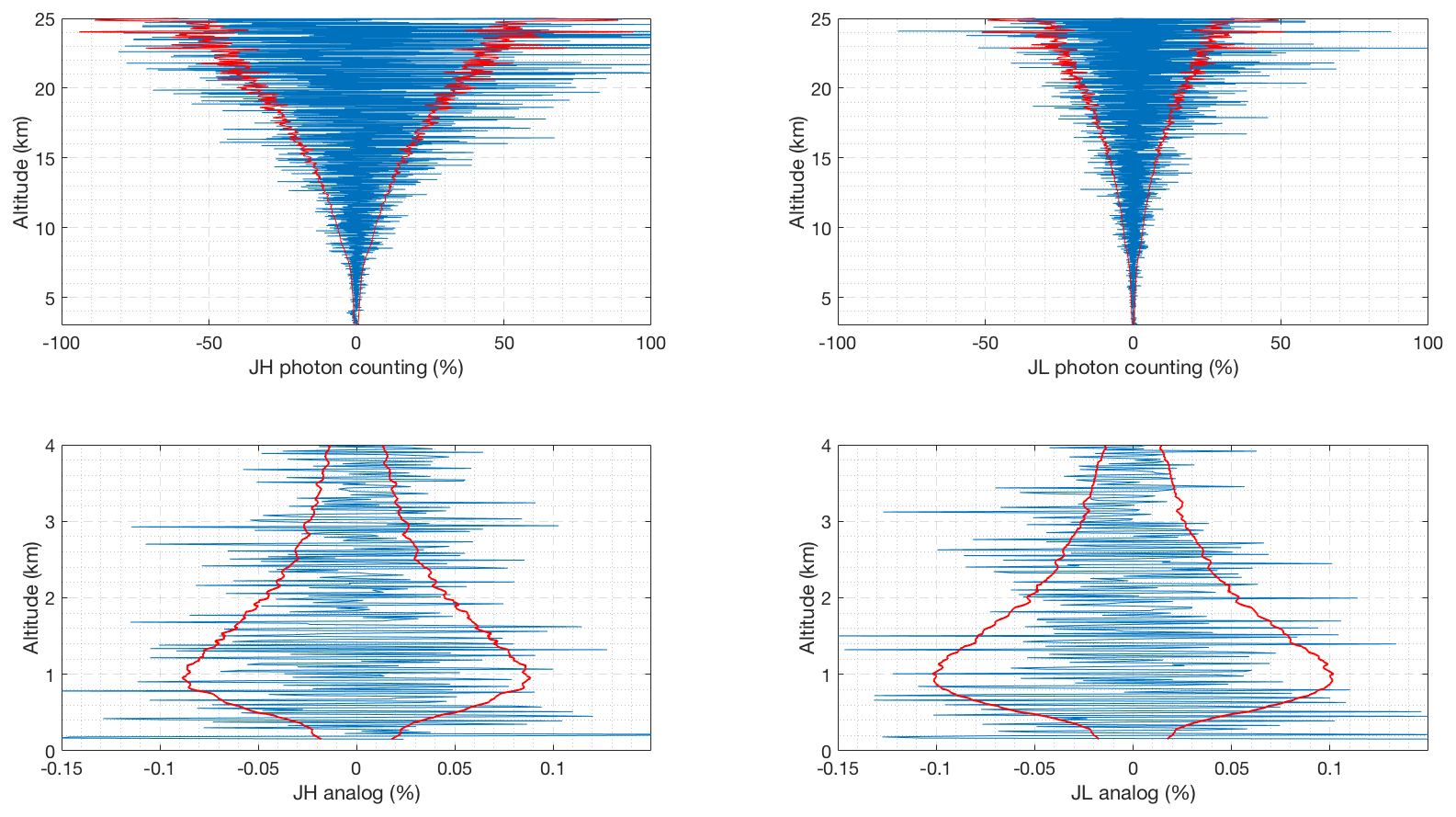
Figure 13Difference between the forward model and the nighttime RALMO measurements on 5 July 2011 with the presence of a cirrus cloud for the four signals (blue). The red curves show the standard deviation of the measurements.
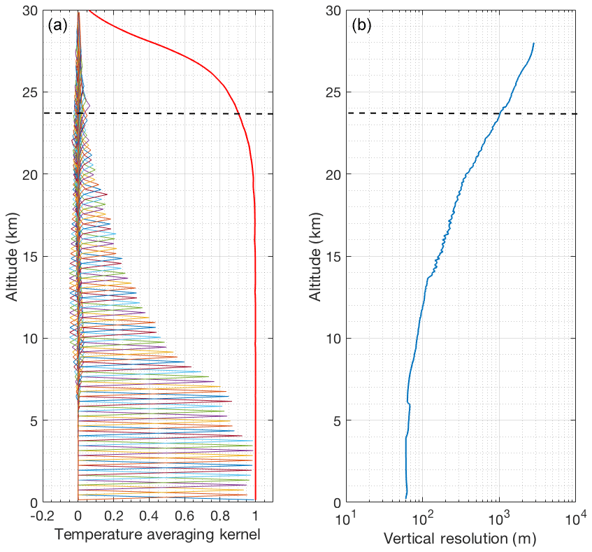
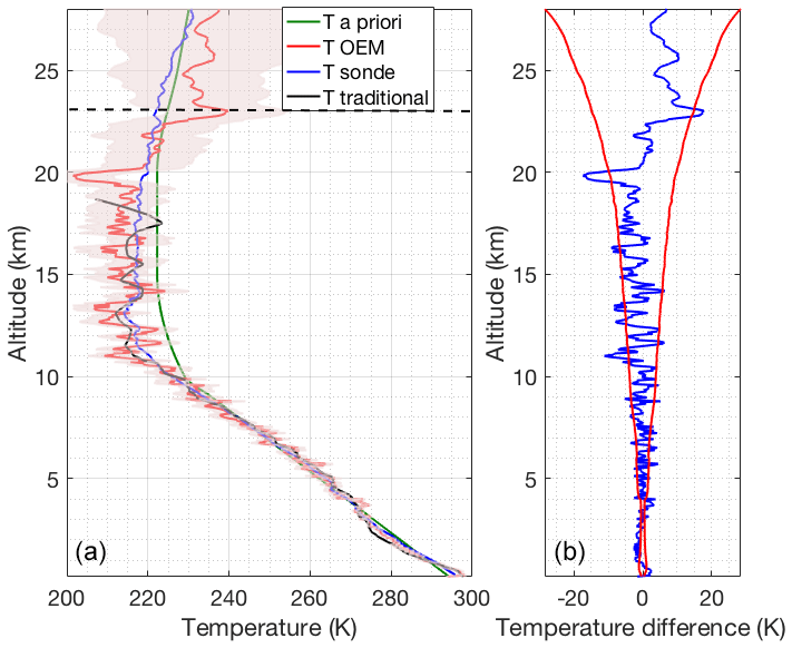
Figure 15Same as Fig. 4 but for 5 July 2011 with a cirrus cloud at 6 km height, using the OEM.
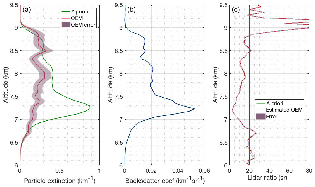
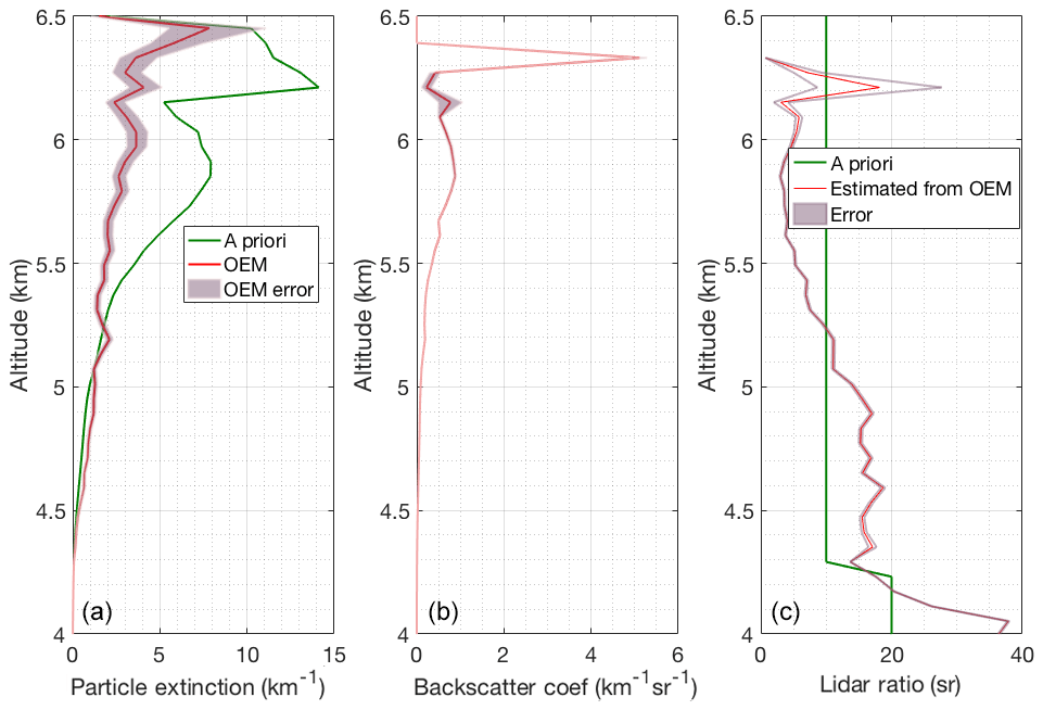
Figure 16(a) Retrieved particle extinction (red) and the a priori particle extinction used in the OEM (green). (b) Backscatter coefficient calculated from the nighttime RALMO measurements on 5 July 2011 with of a cirrus cloud present at 6 km height. (c) Lidar ratio used to determine a priori particle extinction (green) and the estimated lidar ratio using the OEM-retrieved particle extinction (red).
The retrieved geometrical overlap function from the measurement with the cirrus cloud (not shown) agrees within 10 % uncertainty with the geometrical overlap functions retrieved from the measurement with clear sky conditions, as the cloud is above the region of complete geometrical overlap. The red curve in the first plot in Fig. 16 shows the OEM-retrieved particle extinction and the green curve is the a priori particle extinction estimated using the RALMO PRR and elastic measurements, assuming a lidar ratio for cirrus clouds in order to estimate an a priori extinction (Sects. 4, 4.3). Above 6.75 km, the OEM-retrieved particle extinction is around 0.25 km−1 and approximately 2 times smaller than the a priori yielding a lidar ratio of 5–15 sr, while the initial guess was 20 sr (Fig. 16). Ansmann et al. (1992b), using independent measurements of particle extinction and backscatter profiles in cirrus clouds, show similar extinction values (0–0.5 km−1) and also similar values for the lidar ratio inside the cloud, 0–10 sr. Thus, the OEM-retrieved extinctions for this cirrus cloud appear to be reasonable. Below 6.75 km, the lidar ratio is around 20 sr, which could be an indication that this part of the cloud is supercooled liquid.
The uncertainty budget for this case (not shown) is similar to the previous two cases shown; the cloud has little effect on the uncertainty values. As before, the statistical uncertainty makes the largest contribution to the full uncertainty. We have also calculated the statistical uncertainties for the estimated lidar ratio profile by standard uncertainty propagation of the OEM particle extinction and backscatter coefficient statistical uncertainties.
5.4 Case 4: nighttime with lower level cloud
A cloud at about 4 km is present in measurements used for the last case study (Table 3). In this situation we use our OEM-retrieved geometrical overlap during clear conditions as our a priori geometrical overlap profile. We then retrieve geometrical overlap to the cloud base (4 km height) and particle extinction above 4 km. In this case the retrieved geometrical overlap up to 4 km agrees within 10 % uncertainty with the OEM-retrieved geometrical overlap for clear conditions.
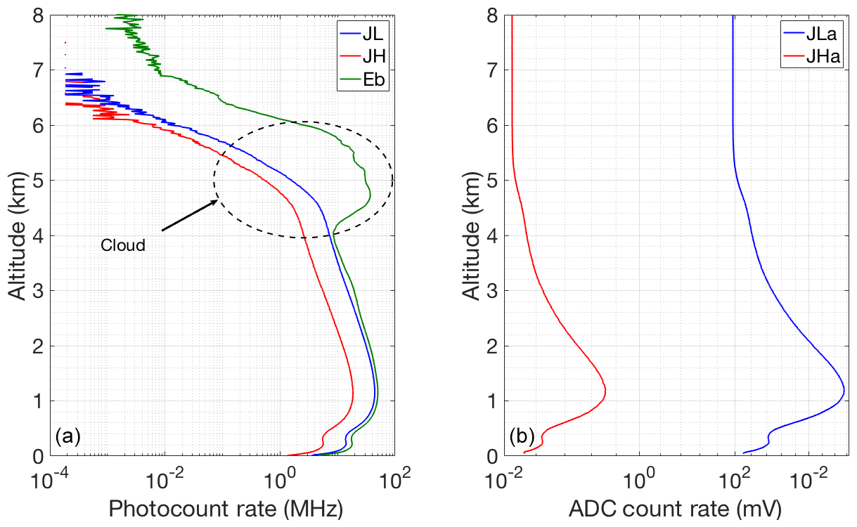
Figure 17Count rate for 30 min of coadded RALMO measurements from 23:00 UT on 21 June 2011, which has a cloud base at an height about 4 km; (a) Photon-counting channels (blue curve, JL; red curve, JH; green, Elastic); (b) Analog channels.
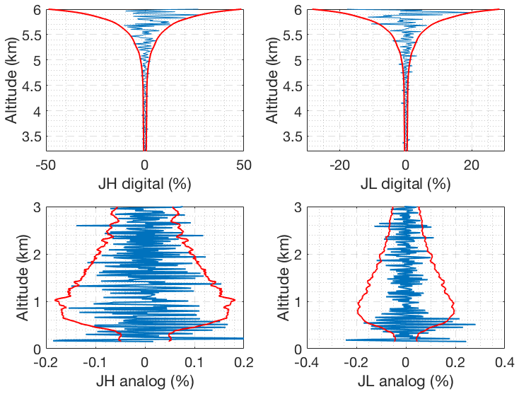
Figure 18Difference between the forward model and the nighttime RALMO measurements on 21 June 2011 with the presence of a lower level cloud for the four signals (blue). The red curves show the standard deviation of the measurements.
Figure 17 shows the measurements in the four PRR channels and the elastic channel measurement (Fig. 17a, green curve). It can be seen in the elastic signal that the cloud base is at around 4 km height. The Raman measurements drop above 4 km and are fully attenuated at 7 km.
We use these measurements obtained during cloudy conditions as input to our OEM and obtain unbiased residuals which fall within the standard deviation of the measurements, meaning the forward model accurately retrieve temperatures in the presence of cloud.
The response function (Fig. 19a) is 0.9 at 6 km, which is considered the maximum height where the OEM-retrieved temperatures are valid. At this height the vertical resolution (Fig. 19b) rapidly increases as the cloud thickens. As shown in Fig. 20b, up to 6 km, the temperature from the sonde launched at 23:00 UT from Payerne and OEM temperature agree with each other within the statistical uncertainty in the OEM temperature. Temperatures retrieved using the traditional method are similar to the OEM and sonde measurements up to 3.5 km, while inside the cloud the traditional temperature starts to deviate.
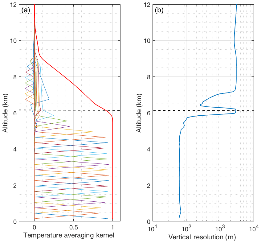
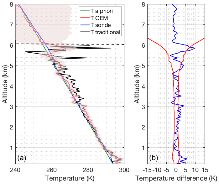
Figure 20Same as Fig. 3 but for 21 June 2011 with the presence of a lower level cloud, using the OEM.
Below 5.25 km the retrieved particle extinction coefficient agrees well with the a priori values and the corresponding lidar ratio is between 15 and 20 sr indicating a liquid cloud. Above 5.25 km the retrieved particle extinction is smaller than the first guess yielding again a lidar ratio around 5 sr (Fig. 21a). This could be an indication that the cloud became an ice cloud above 5.25 km.
The four retrievals discussed in the previous section demonstrate that the OEM provides robust and accurate retrievals of temperature, geometrical overlap, and particle extinction coefficients during clear conditions in both daytime and nighttime and in high-cloud and low-cloud nighttime conditions. Unlike the traditional Raman lidar temperature analysis method (Cooney, 1972; Arshinov et al., 1983; Di Girolamo et al., 2004; Behrendt, 2005; Zuev et al., 2017), the OEM does not require an analytic form of a calibration function; rather a single calibration coefficient has to be estimated using a reference temperature profile and this was shown to have a small effect on the retrieved temperature.
The calibration function plays a key role in the traditional temperature retrieval algorithm from the PRR backscattered signals, in particular if calibration is not done over the entire observed temperature range. Typically, a calibration function linear in 1∕T is used for systems that detect only one or multiple RR lines (Behrendt, 2005), although other forms of calibration functions have been employed. Recently, Zuev et al. (2017) showed closer agreement at times when the temperature calculation used a higher-order polynomial for the calibration function. All calibration coefficient estimation methods require multiple reference data points which span ideally the entire range of temperatures to avoid extrapolation errors.
The only calibration required in our OEM scheme is the determination of the two coupling constants, R and Ra. The coupling constants can be estimated at a specific height (that is over a narrow range of temperature) without introducing extrapolation errors. Using the OEM we can show that the contribution of the coupling constant to the temperature uncertainty is on the order of 0.07 K in the height below 4 km and about 0.2 K or less above 4 km for a wide variety of sky conditions.
The OEM temperature retrievals of four very different sky conditions have been compared against coincident radiosonde temperature measurements. The case presented is the US Standard Model normalized to the surface temperature from the coincident sonde temperature. We successfully used other a priori temperature profiles, such as the smoothed sonde temperature measurements and temperature from the Mass Spectrometer and Incoherent Scatter (MSIS) radar model, to retrieve temperature using our OEM algorithm. All the retrieved temperature profiles using each a priori profile for heights where the response function is 0.9 or greater are identical within the statistical uncertainty.
In our study, we have successfully retrieved a geometrical overlap function for the RALMO system using the PRR measurements simultaneously with the temperature retrieval. Ray-tracking studies have concluded that the RALMO system reaches its full geometrical overlap by 5.0–5.5 km in height. These calculations are consistent with our geometrical overlap retrievals in both clear daytime and nighttime conditions. Measuring the geometrical overlap function and its uncertainty allows a more accurate estimation of the particle extinction coefficient when clouds or aerosols are present. The particle extinction profiles we retrieved in the two cloudy condition cases are consistent with measurements collected by Ansmann and Müller (2005) for cirrus clouds and with O'Connor et al. (2004) for liquid clouds.
The particle extinction coefficient is retrieved in the full geometrical overlap region, i.e. above 6 km or above the cloud base. The extinction values and lidar ratios we obtained for high and mid-level clouds are in agreement with other publications. The two case studies featuring clouds suggest that both clouds consisted of a liquid and a ice part with lidar ratios at 18 and 5 sr.
For all the case studies we presented, the lidar constants for the lower quantum channels (analog and photon counting), the dead times for each photon-counting channel (JL and JH), and background for all four signals are also retrieved. The retrieved lidar constants for each channel agreed within 20 % uncertainty for all four cases. The retrieved dead times are about 3.8 ns and consistent with the dead times specified by the manufacturer and other independent estimates.
The uncertainty budget provided by the OEM contains both random and systematic uncertainties. Estimation of the uncertainty budget requires assignment of appropriate covariances to the model parameters. Using the standard deviations given in Table 2, the uncertainty budgets for all the case studies are estimated. The largest contribution towards the temperature uncertainty originates from the statistical uncertainty due to the measurement noise. Overall contribution from the coupling constants to the temperature uncertainty are less than 0.2 K for all heights. Given the fact that the measurement noise can be reduced with longer integration times, this result suggests that by the OEM method very precise temperature measurements are possible even if calibration is only possible over a small temperature range.
The systematic uncertainties of pressure and air density are on the order of 0.1 K and 0.1 mK, respectively. Understanding the full uncertainty budget of temperature is of particular importance for trend analysis and process studies. The observational basis for supersaturation studies in the upper troposphere is still unsatisfactory and the OEM framework allows us to combine different data sources to provide a high-quality data set including profile-by-profile uncertainty budgets.
We have demonstrated the ability of the OEM to retrieve multiple geophysical and instrumental parameters from PRR lidar measurements. The first-principle forward model adequately represents the raw PRR measurement and allows us to retrieve temperature, geometrical overlap, particle extinction, lidar constants, background counts, and dead time using multiple analog and photon-counting channels. We found the following results from our OEM temperature retrievals from PRR measurements:
-
The forward model presented, based on the lidar equation, contains the essential physics to reproduce the analog and photon-counting measurements, leading to unbiased residuals and robust estimates of temperature.
-
Our OEM retrieval does not require a calibration function as used in the traditional temperature retrieval method. It only requires determination of the two coupling constants, R and Ra, using a reference temperature profile that can be estimated at a specific height bin (or over a range). Retrieved temperature profiles from both daytime and nighttime raw PRR measurements in clear and cloudy conditions agree well with coincident radiosonde measurements.
-
The OEM provides a cutoff height for the temperature retrievals that specify up to which height the retrieved profile is primarily due to the measurements and not the a priori temperature profile.
-
Vertical resolution is determined at each height and is automatically adapted in the retrieval in response to increasing measurement noise with height.
-
The OEM provides a complete uncertainty budget, including random and systematic uncertainties due to model parameters, including the assumed pressure, air density, and the coupling constants.
-
Simultaneous analog, which are linear, and photon-counting measurements allow the dead time to be retrieved.
-
The OEM-retrieved geometrical overlap function for the RALMO using the measurements in clear conditions is determined and shown to be consistent with, but not the same as, that calculated by Dinoev et al. (2013). Hence, retrievals of the particle extinction coefficient are possible using the OEM from the measurements in cloudy conditions or when aerosol layers are present.
-
The OEM is a computationally fast and practical method for routine temperature retrievals from lidar measurements as required for operational lidar systems.
We have demonstrated that the OEM allows for retrieval of temperature from pure rotational Raman lidar measurements that are consistent with the coincident sonde temperature. We discussed the advantages of the OEM over the traditional temperature retrieval algorithm. We can use the OEM-retrieved temperature to study temperature trends with the benefit of a full uncertainty budget provided by our OEM. Our OEM temperature retrieval can also be used for routine measurements in a wide variety of observing conditions, and is applicable to any similar PRR lidar system.
We are in the process of implementing the OEM for routine temperature measurements from the RALMO system. We are also combining the OEM PRR temperature retrieval with the OEM water vapour mixing ratio retrieval of Sica and Haefele (2016) to directly retrieve relative humidity from the RALMO measurements, both for its importance to operational forecasting and to allow the study of ice supersaturation events. We are also assimilating ERA5 hourly reanalysis data into the OEM relative humidity and temperature algorithm to improve the accuracy of the OEM relative humidity retrievals.
Measurements used in this paper may be requested from MeteoSwiss by contacting Alexander Haefele (alexander.haefele@meteoswiss.ch).
SMG was responsible for coding the Raman temperature OEM routine as well as the comparisons between the OEM and radiosonde measurements. She also wrote the initial draft of the paper. RJS and AH were SMG's PhD supervisors. They defined the project and participated in the development of the OEM code. AH and GM provided lidar and radiosonde measurements and performed the traditional method to estimate the temperature from the measurements.
The authors declare that they have no conflict of interest.
We thank Ghazal Farhani for her helpful comments and suggestions that were extremely useful to us. We also thank the Western University Writing Support Centre and Patricia Sica for their assistance in editing and proofreading this paper. This project has been funded in part by the National Science and Engineering Research Council of Canada and by the Canadian Space Agency under the Arctic Validation and Training for Atmospheric Research in Science (AVATARS) program.
This project has been funded in part by the National Science and Engineering Research Council of Canada through a Discovery Grant (Robert J. Sica) and a CREATE award for a Training Program in Arctic Atmospheric Science (Kimberly Strong, U Toronto, PI) and by MeteoSwiss (Switzerland).
This paper was edited by Gerd Baumgarten and reviewed by Christoph Ritter and one anonymous referee.
Adam, S., Behrendt, A., Schwitalla, T., Hammann, E., and Wulfmeyer, V.: First assimilation of temperature lidar data into an NWP model: impact on the simulation of the temperature field, inversion strength and PBL depth, Q. J. Roy. Meteorol. Soc., 142, 2882–2896, 2016. a
Ansmann, A. and Müller, D.: Lidar and atmospheric aerosol particles, in: Lidar, 105–141, Springer, New York, 2005. a
Ansmann, A., Riebesell, M., Wandinger, U., Weitkamp, C., Voss, E., Lahmann, W., and Michaelis, W.: Combined Raman elastic-backscatter lidar for vertical profiling of moisture, aerosol extinction, backscatter, and lidar ratio, Appl. Phys. B, 55, 18–28, 1992a. a
Ansmann, A., Wandinger, U., Riebesell, M., Weitkamp, C., and Michaelis, W.: Independent measurement of extinction and backscatter profiles in cirrus clouds by using a combined Raman elastic-backscatter lidar, Appl. Opt., 31, 7113–7131, 1992b. a
Arshinov, Y. F., Bobrovnikov, S., Zuev, V. E., and Mitev, V.: Atmospheric temperature measurements using a pure rotational Raman lidar, Appl. Opt., 22, 2984–2990, 1983. a
Behrendt, A.: Temperature measurements with lidar, in: Lidar, 273–305, Springer, New York, 2005. a, b, c, d, e, f, g
Behrendt, A., Nakamura, T., Onishi, M., Baumgart, R., and Tsuda, T.: Combined Raman lidar for the measurement of atmospheric temperature, water vapor, particle extinction coefficient, and particle backscatter coefficient, Appl. Opt., 41, 7657–7666, 2002. a
Bucholtz, A.: Rayleigh-scattering calculations for the terrestrial atmosphere, Appl. Opt., 34, 2765–2773, 1995. a
Cooney, J.: Measurement of atmospheric temperature profiles by Raman backscatter, J. Appl. Meteorol., 11, 108–112, 1972. a, b
Di Girolamo, P., Marchese, R., Whiteman, D., and Demoz, B.: Rotational Raman Lidar measurements of atmospheric temperature in the UV, Geophys. Res. Lett., 31, L01106, 2004. a
Dinoev, T., Simeonov, V., Calpini, B., and Parlange, M.: Monitoring of Eyjafjallajökull ash layer evolution over payerne Switzerland with a Raman lidar, Proceedings of the TECO, 2010. a, b, c
Dinoev, T., Simeonov, V., Arshinov, Y., Bobrovnikov, S., Ristori, P., Calpini, B., Parlange, M., and van den Bergh, H.: Raman Lidar for Meteorological Observations, RALMO – Part 1: Instrument description, Atmos. Meas. Tech., 6, 1329–1346, https://doi.org/10.5194/amt-6-1329-2013, 2013. a, b, c
Eriksson, P., Jiménez, C., and Buehler, S. A.: Qpack, a general tool for instrument simulation and retrieval work, J. Quant. Spectrosc. Ra., 91, 47–64, 2005. a, b, c
Farhani, G., Sica, R. J., Godin-Beekmann, S., Ancellet, G., and Haefele, A.: Improved ozone DIAL retrievals in the upper troposphere and lower stratosphere using an optimal estimation method, Appl. Opt., 58, 1374–1385, https://doi.org/10.1364/AO.58.001374, 2019. a
He, J., Chen, S., Zhang, Y., Guo, P., and Chen, H.: A Novel Calibration Method for Pure Rotational Raman Lidar Temperature Profiling, J. Geophys. Res.-Atmos., 123, 10–925, 2018. a
Herzberg, G.: Molecular spectra and molecular structure, vol. 1, Read Books Ltd, Redditch, 2013. a
Lenschow, D. H., Wulfmeyer, V., and Senff, C.: Measuring second-through fourth-order moments in noisy data, J. Atmos. Ocean Tech., 17, 1330–1347, 2000. a
Mattis, I., Ansmann, A., Althausen, D., Jaenisch, V., Wandinger, U., Müller, D., Arshinov, Y. F., Bobrovnikov, S. M., and Serikov, I. B.: Relative-humidity profiling in the troposphere with a Raman lidar, Appl. Opt., 41, 6451–6462, 2002. a
NASA: United States standard atmosphere, US Government Printing Office, pp. 1–227, NASA-TM-X-74335, NOAA-S/T-76-1562, 1976. a
Nicolet, M.: On the molecular scattering in the terrestrial atmosphere: An empirical formula for its calculation in the homosphere, Planet. Space Sci., 32, 1467–1468, 1984. a, b
O'Connor, E. J., Illingworth, A. J., and Hogan, R. J.: A Technique for Autocalibration of Cloud Lidar, J. Atmos. Ocean. Tech., 21, 777–786, https://doi.org/10.1175/1520-0426(2004)021<0777:ATFAOC>2.0.CO;2, 2004. a
Pappalardo, G., Amodeo, A., Pandolfi, M., Wandinger, U., Ansmann, A., Bösenberg, J., Matthias, V., Amiridis, V., De Tomasi, F., Frioud, M., Iarlori, M., Komguem, L., Papayannis, A., Rocadenbosch, F., and Wang, X.: Aerosol lidar intercomparison in the framework of the EARLINET project, 3. Raman lidar algorithm for aerosol extinction, backscatter, and lidar ratio, Appl. Opt., 43, 5370–5385, 2004. a
Penney, C., Peters, R. S., and Lapp, M.: Absolute rotational Raman cross sections for N2, O2, and CO2, JOSA, 64, 712–716, 1974. a
Povey, A. C., Grainger, R. G., Peters, D. M., and Agnew, J. L.: Retrieval of aerosol backscatter, extinction, and lidar ratio from Raman lidar with optimal estimation, Atmos. Meas. Tech., 7, 757–776, https://doi.org/10.5194/amt-7-757-2014, 2014. a
Povey, A. C., Grainger, R. G., Peters, D. M., Agnew, J. L., and Rees, D.: Estimation of a lidar’s overlap function and its calibration by nonlinear regression, Appl. Opt., 51, 5130–5143, 2012. a
Radlach, M., Behrendt, A., and Wulfmeyer, V.: Scanning rotational Raman lidar at 355 nm for the measurement of tropospheric temperature fields, Atmos. Chem. Phys., 8, 159–169, https://doi.org/10.5194/acp-8-159-2008, 2008. a, b
Reichardt, J., Wandinger, U., Klein, V., Mattis, I., Hilber, B., and Begbie, R.: RAMSES: German Meteorological Service autonomous Raman lidar for water vapor, temperature, aerosol, and cloud measurements, Appl. Opt., 51, 8111–8131, 2012. a
Rodgers, C. D.: Inverse methods for atmospheric sounding: theory and practice, vol. 2, World scientific, Singapore, 2000. a, b, c, d
Sica, R. and Haefele, A.: Retrieval of temperature from a multiple-channel Rayleigh-scatter lidar using an optimal estimation method, Appl. Opt., 54, 1872–1889, 2015. a, b
Sica, R. and Haefele, A.: Retrieval of water vapor mixing ratio from a multiple channel Raman-scatter lidar using an optimal estimation method, Appl. Opt., 55, 763–777, 2016. a, b, c
Wang, Y., Hua, D., Mao, J., Wang, L., and Xue, Y.: A detection of atmospheric relative humidity profile by UV Raman lidar, J. Quant. Spectrosc. Ra., 112, 214–219, 2011. a
Weng, M., Yi, F., Liu, F., Zhang, Y., and Pan, X.: Single-line-extracted pure rotational Raman lidar to measure atmospheric temperature and aerosol profiles, Opt. Express, 26, 27555–27571, https://doi.org/10.1364/OE.26.027555, 2018. a, b
Whiteman, D. N.: Examination of the traditional Raman lidar technique, I, Evaluating the temperature-dependent lidar equations, Appl. Opt., 42, 2571–2592, 2003. a
Yan, Q., Wang, Y., Gao, T., Gao, F., Di, H., Song, Y., and Hua, D.: Optimized retrieval method for atmospheric temperature profiling based on rotational Raman lidar, Appl. Opt., 58, 5170–5178, 2019. a
Zuev, V. V., Gerasimov, V. V., Pravdin, V. L., Pavlinskiy, A. V., and Nakhtigalova, D. P.: Tropospheric temperature measurements with the pure rotational Raman lidar technique using nonlinear calibration functions, Atmos. Meas. Tech., 10, 315–332, https://doi.org/10.5194/amt-10-315-2017, 2017. a, b, c
- Abstract
- Introduction
- The RAman Lidar for Meteorological Observations
- The PRR lidar equation
- Application of the OEM for PRR temperature retrieval
- Results from the temperature retrieval
- Discussion
- Conclusions
- Data availability
- Author contributions
- Competing interests
- Acknowledgements
- Financial support
- Review statement
- References