the Creative Commons Attribution 4.0 License.
the Creative Commons Attribution 4.0 License.
 | 22 Nov 2019
A new laser-based and ultra-portable gas sensor for indoor and outdoor formaldehyde (HCHO) monitoring
Norton T. Allen
Thomas F. Hanisco
Glenn M. Wolfe
Jason M. St. Clair
Frank N. Keutsch
In this work, a new commercially available, laser-based, and ultra-portable formaldehyde (HCHO) gas sensor is characterized, and its usefulness for monitoring HCHO mixing ratios in both indoor and outdoor environments is assessed. Stepped calibrations and intercomparison with well-established laser-induced fluorescence (LIF) instrumentation allow a performance evaluation of the absorption-based, mid-infrared HCHO sensor from Aeris Technologies, Inc. The Aeris sensor displays linear behavior (R2 > 0.940) when compared with LIF instruments from Harvard and NASA Goddard. A nonlinear least-squares fitting algorithm developed independently of the sensor's manufacturer to fit the sensor's raw absorption data during post-processing further improves instrument performance. The 3σ limit of detection (LOD) for 2, 15, and 60 min integration times are 2190, 690, and 420 pptv HCHO, respectively, for mixing ratios reported in real time, though the LOD improves to 1800, 570, and 300 pptv HCHO, respectively, during post-processing. Moreover, the accuracy of the sensor was found to be ± (10 % + 0.3) ppbv when compared against LIF instrumentation sampling ambient air. The aforementioned precision and level of accuracy are sufficient for most HCHO levels measured in indoor and outdoor environments. While the compact Aeris sensor is currently not a replacement for the most sensitive research-grade instrumentation available, its usefulness for monitoring HCHO is clearly demonstrated.
- Article
(3819 KB) -
Supplement
(354 KB) - BibTeX
- EndNote


Understanding the production and lifetime of molecules formed from oxidation chemistry is essential to our understanding of atmospheric chemistry as a whole. Formaldehyde (HCHO) is one of the most ubiquitous tracers of volatile organic compound (VOC) oxidation chemistry since it is generally formed when VOCs are oxidized by compounds such as OH, O3, and NO3 (Seinfeld and Pandis, 2016). The measurement of HCHO in situ and via satellite is thus extensively used by models to constrain VOC emissions from both biogenic and anthropogenic sources worldwide and to test our understanding of VOC oxidation chemistry (Choi et al., 2010; Chan Miller et al., 2017; Zhu et al., 2017b).
While atmospheric HCHO is primarily produced from the oxidation of VOCs (such as isoprene and CH4), it is also produced via fuel combustion and biomass burning (Anderson et al., 1996; Holzinger et al., 1999). In the indoor environment, HCHO is released from building materials and cleaning products (Nazaroff and Weschler, 2004), and normal HCHO mixing ratios are generally higher indoors (ranging from 5 to 40 ppbv) than those measured outdoors (ranging from 0.5 to 15 ppbv with rural areas being on the lower end of the range and urban areas on the higher end) (Salthammer, 2013). Given that individuals generally spend ∼90 % of their time indoors (Klepeis et al., 2001) and that the United States Environmental Protection Agency (U.S. EPA) classifies HCHO as a hazardous air pollutant and probable human carcinogen (Baucus, 1990; U.S. Environmental Protection Agency, 2018), the measurement of HCHO indoors is just as essential as its measurement outdoors. Recently, it has been estimated that 6600–12 500 people in the US will develop cancer over their lifetime due to outdoor HCHO exposure (Zhu et al., 2017a), which implies that the number from indoor exposure should be substantially higher. The current recommended exposure limit by the National Institute for Occupational Health and Safety (NIOSH) is a time-weighted average of 16 ppbv HCHO for a 10 h workday during a 40 h workweek (Centers for Disease Control and Prevention, 2007).
Numerous chemical, spectrometric, and spectroscopic methods have been developed and utilized for the accurate and precise in situ measurement of gas-phase HCHO. Table 1 summarizes several research-grade HCHO instruments developed over the past few decades listing their accuracies as well as limits of detection (3σ) and corresponding integration times. All methods can achieve sub-parts-per-billion-by-volume detection limits within their specified integration times and accuracies better than or equal to 15 %. Of all the methods, the measurement of HCHO by laser-induced fluorescence (LIF) achieves the best detection limit with the shortest integration time. Additionally, chemical derivatization is currently employed as a standard by the U.S. EPA: The current methodology (TO–11A; second edition) for determining HCHO mixing ratios instructs users to sample ambient air with pre-coated DNPH (2,4-dinitrophenylhydrazine) cartridges and then ship these cartridges to a laboratory for analysis of the formaldehyde–DNPH derivative by high-performance liquid chromatography (HPLC) (Winberry et al., 1999).
Table 1Overview of selected in situ HCHO measurement techniques.
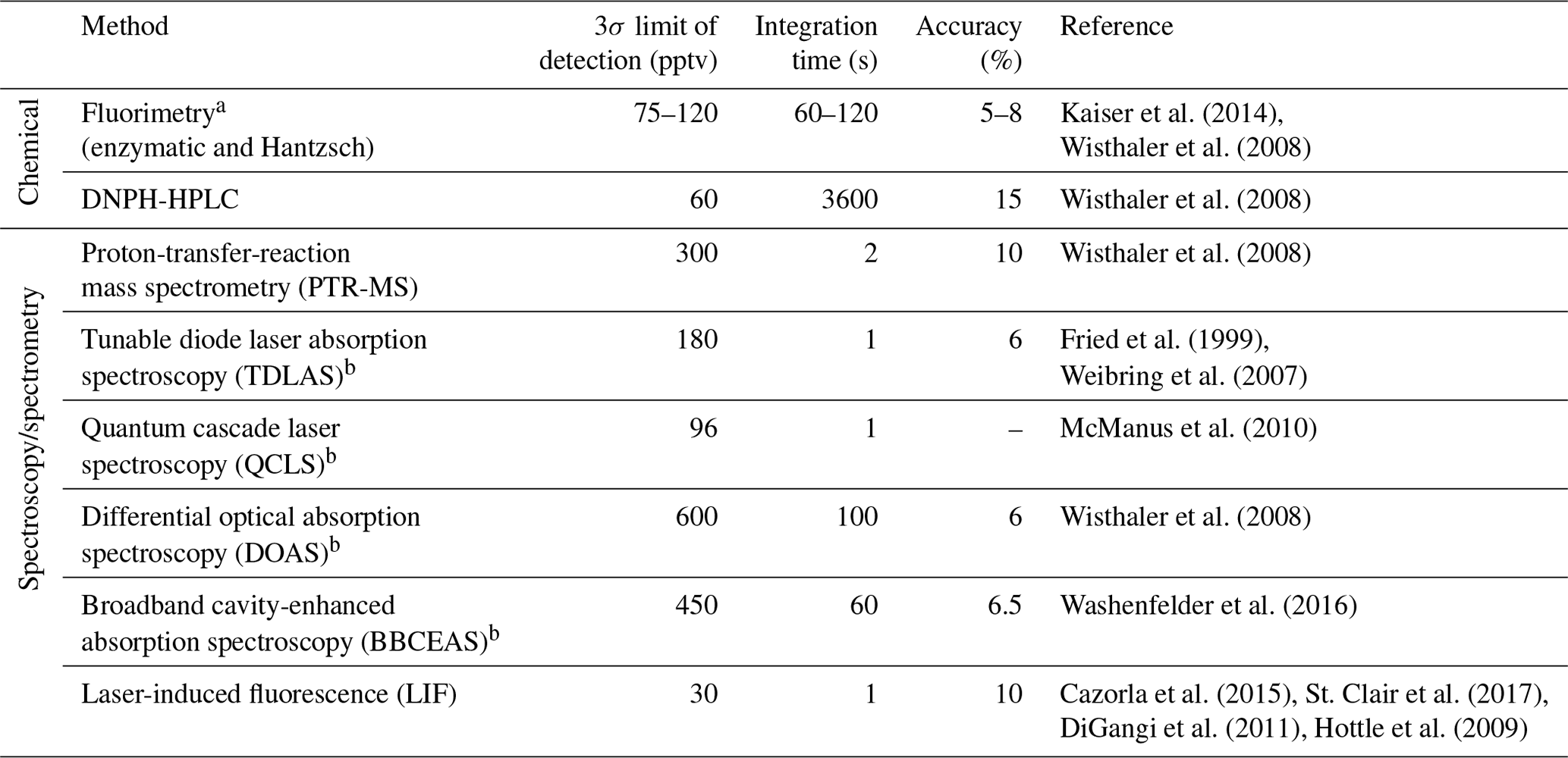
a Specified values are for Hantzsch. b The path lengths of the astigmatic Herriott cell in the TDLAS and QCLS instruments are 100 and 200 m, respectively. The DOAS instrument has a light path of 960 m, and the BBCEAS instrument has an effective path length of 1430 m.
Even though these research-grade methods produce high-quality scientific data, they also require large investments of money, power, and operator time. Mass spectrometric methods have high power requirements, are large, are sensitive to humidity effects for the measurement of HCHO, and have possible cross-sensitivities (for any fragment with the same mass-to-charge ratio as ionized HCHO) (Kaiser et al., 2014; Vlasenko et al., 2010). Chemical methods suffer from reproducibility problems at ambient mixing ratios, are labor and time intensive, and require the use of acidic or hazardous reagents. Current laser-based instruments using methods such as LIF, TDLAS, QCLS, and DOAS have sufficient specifications but need knowledgeable operators and are not particularly suitable for widespread adoption in sensor networks. For applications that require a large number of instruments (such as monitoring networks), or the ability to easily and cheaply move instrumentation around from location to location (such as for studying indoor air chemistry), a smaller and easier-to-operate HCHO sensor that still compares well against research-grade instrumentation with respect to accuracy is preferable.
Toward this purpose, we characterize a new mid-IR laser-based HCHO sensor (Pico series) from Aeris Technologies to quantify its performance against some of the best available research-grade instrumentation (i.e., LIF). Through laboratory experiments, the sensor's Allan–Werle deviation curves are calculated to determine the optimal averaging time for HCHO measurements and to assess the sensor's true 3σ limit of detection. The sensor is subsequently compared against LIF instrumentation from NASA and Harvard as a proxy for the sensor's accuracy. Finally, sensor measurements from both outdoor and indoor environments are shown to display the sensor's usefulness for monitoring HCHO.
The sensor as supplied has external dimensions of () and a weight of 3 kg (including batteries). A proprietary folded Herriott detection cell (Paul, 2019) inside the instrument has a 1300 cm path length, a volume of 60 cm3, and dimensions of () (Fig. 1 with a simple schematic in Fig. S1 in the Supplement). The pumping speed is 750 standard cubic centimeters per minute (sccm) to maintain a constant pressure of 250 mbar and a residence time of 5 s inside the detection cell. The 6 h battery life, onboard GPS, and 15 W power consumption make the sensor highly portable and thus particularly useful for mobile and field measurements. The sensor is networkable and easy to operate, and HCHO mixing ratios can be monitored via remote desktop over the sensor's Wi-Fi network.
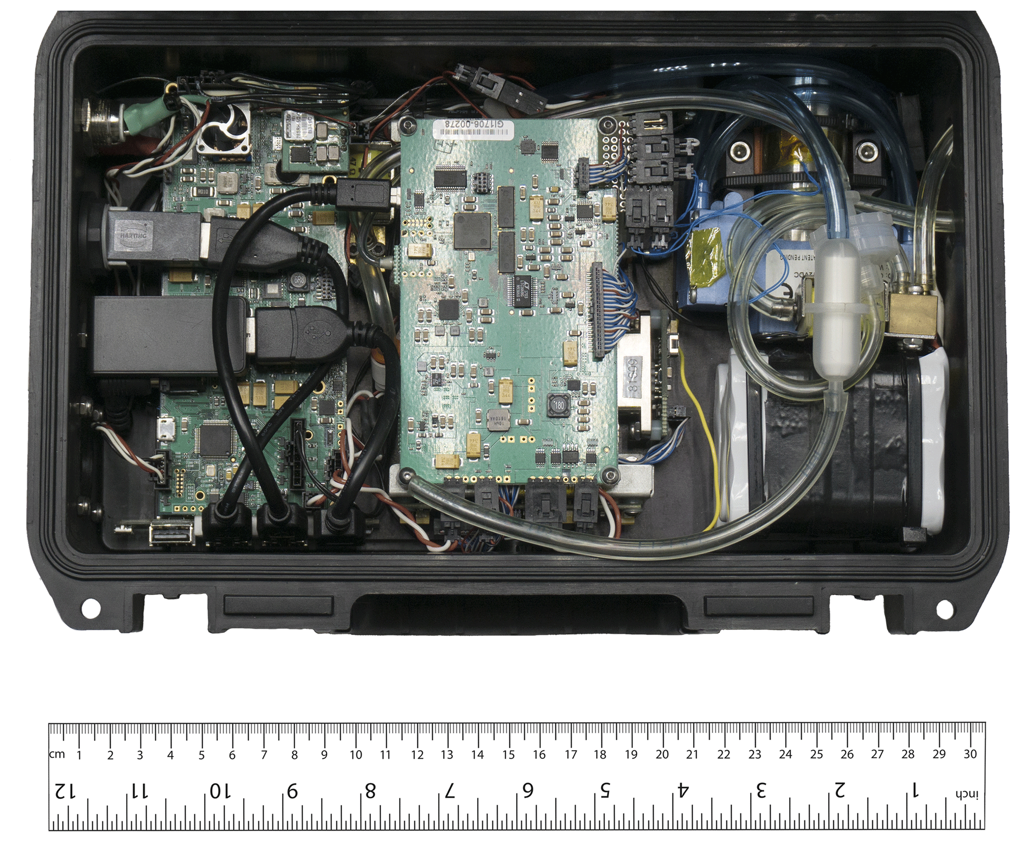
Figure 1Internal view of the mid-IR, absorption-based HCHO sensor from Aeris Technologies. The sensor fits inside a Pelican case that provides for easy transport and mobility.
Using a proprietary fast-fitting routine that has been optimized to report HCHO and H2O mixing ratios in real time (subsequently referred to as the Aeris Real-time (ART) fit), the sensor fits a rovibrational line of HCHO at 2831.6413 cm−1 (with a corresponding line intensity of cm−1 ∕ (molecule ⋅ cm−2)) that matches the transition chosen for the TDLAS system in Fried et al. (1999). A search of the nearby spectral region using HITRAN (an acronym for the high-resolution transmission molecular absorption database) shows this region to be free of strong spectral interferences from other molecular absorbers that would completely prevent the HCHO line from being fit under normal operating conditions (Gordon et al., 2017; Rothman et al., 2013). Additionally, ART fit uses a nearby rovibrational line of an isotopologue of water (HDO) located at 2831.8413 cm−1 (3.014 × 10⁻²⁴ cm−1 ∕ (molecule ⋅ cm−2)) as a spectral reference to find and fit the previously mentioned HCHO spectral feature. The HCHO line is reliably found when the mixing ratio of H2O is above 2000 ppmv (corresponding to relative humidities of 6 %, 12 %, and 33 % at temperatures of 25, 15, and 0 ∘C, respectively). The HDO reference line, strongest HCHO spectral feature, and fringes caused by etalons in the optical train are observed in the baseline-subtracted signal depicted in Fig. 2.
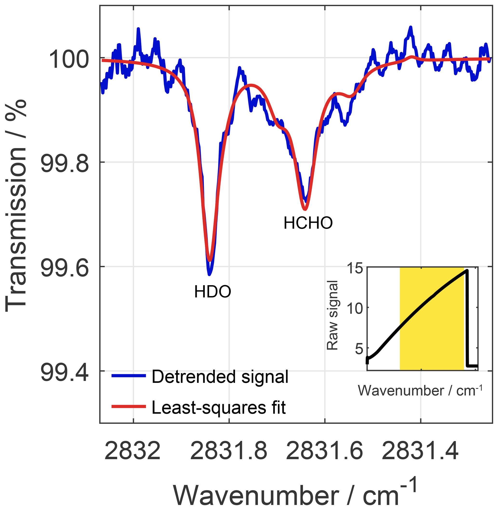
Figure 2When the H2O mixing ratio is above 2000 ppmv, the HDO line at 2831.8413 cm−1 rises above the fringing caused by etalons in the detection cell so that the position of the HCHO line at 2831.6413 cm−1 can be reliably located and the spectral line fit. The fit depicted corresponds to a HCHO mixing ratio around 800 ppbv. The inset shows the 1 Hz raw data from the sensor before baseline subtraction. The yellow shaded region corresponds to the wavelength range being fit.
The raw signal shown in the inset of Fig. 2 is reported at a rate of 1 Hz, and the Beer–Lambert law is used to calculate rudimentary mixing ratios of HCHO and H2O after baseline subtraction. The sensor also employs a two-inlet design and three-way valve system that allows for the measurement and subtraction of a zero during data collection. Using default settings, the three-way valve cycles between the two external inlets every 30 s. Thus, for 15 s, air flow is directed through the sample inlet, which allows air to directly flow into the detection cell after passing through a particle filter. For the other 15 s, the air flow is directed into the zero inlet containing an inline DNPH cartridge (LpDNPH S10L cartridge, Sigma-Aldrich) that filters out all aldehydes, including more than 99 % HCHO, from the air flow before it passes through the particle filter and detection cell. Since a zero is effectively calculated every other 15 s with default settings, the inlet and valve setup employed by the sensor helps to minimize the effects of thermal drift and other background effects (such as outgassing) on the reported HCHO mixing ratio. For instance, since the period of the fringes caused by the etalons in the optical train has a linewidth comparable to the spectral lines being fit, the regular zeroing helps to subtract out the fringes.
The true mixing ratio of HCHO in the sample air over a complete cycle of air flowing through the sample and zero inlets is then defined as the average of the rudimentary 1 Hz HCHO mixing ratios through the sample inlet minus the average of the rudimentary 1 Hz HCHO mixing ratios through the zero inlet for the time period immediately preceding and following the sample inlet:
For the purpose of eliminating any hysteresis effects from the inlet previously being sampled, the first 7 s of data are ignored for each 15 s inlet sampling period. With this definition, the shortest integration time possible using default settings is 30 s. Equation (1) is subsequently used for all HCHO mixing ratios reported by the Aeris sensor.
In this paper, the particle filter was a PTFE filter membrane from Savillex (13 mm ø, 1–2 µm pore size). A spectral interference from newly opened DNPH cartridges was also observed, but this disappears after 2–4 h of continuous sampling. Moreover, the cartridges last anywhere from a few days to a week of continuous use depending on sampling conditions and levels of HCHO encountered.
While ART fit is compatible with the sensor's limited onboard computing resources to calculate HCHO mixing ratios in real time, the sensor also offers the option of outputting its raw 1 Hz spectral data. These raw data were used as input into a repurposed and modified nonlinear least-squares fitting program originally developed for the Harvard integrated cavity output spectroscopy (ICOS) instrument (Sayres et al., 2009) in order to extend the fitting capabilities of the sensor, improve the sensor's performance in very dry conditions, and also have an open-source alternative to ART fit. Based on the Levenberg–Marquardt algorithm to fit absorption spectra, HAPP fit includes optional formulations supporting nonlinear tuning rates typical of laser photodiodes, standard fits for fixed-path-length absorption cells, and a variety of options for fitting the baseline power curve and etalons of the Aeris sensor. Spectral parameters (such as the line position or the Doppler and Lorentz widths for each transition) are dynamically fixed or floated depending on a specified threshold, and spectral lines of the same molecular species are grouped together to better constrain the final fit. All spectral line information can be easily sourced from the HITRAN database. While HAPP fit itself is written in C, the program is supported by a suite of MATLAB scripts to assist in setting up the necessary configuration files from the Aeris raw data and to process the output of HAPP fit into finalized HCHO mixing ratios.
Using HAPP fit, several additional HITRAN lines were fit in addition to the spectral lines used by the ART fit. While a full list of fitted spectral lines is provided in Table S1, we notably fit the CH4 line at 2831.9199 cm−1 (1.622 × 10⁻²¹ cm−1 ∕ (molecule ⋅ cm−2)). When the absolute water content of the sampled air becomes too low (i.e., when H2O < 2000 ppmv – such as during a dry and cold winter), using the previously mentioned HDO line to lock onto the HCHO line becomes impractical. In this case, we found that a small flow (< 1 sccm) of ultrapure CH4 (chemically pure 99.5 % methane; Airgas) can be added to the inlet line, and the CH4 line at 2831.9199 cm−1 can then be used as a spectral reference to find and fit HCHO at 2831.6413 cm−1. The instrument is considered to run in “CH4 mode” only when methane is explicitly added to the gas stream; otherwise, the instrument normally uses the water already present in air to run in “HDO mode”. CH4 mode is currently only available in HAPP fit, though a user-controlled software switch between the two modes might be added in a future update of the Aeris sensor.
4.1 Precision: Allan–Werle deviation and limit of detection (LOD)
The precision of the sensor was calculated for various integration times when running the Aeris sensor in both HDO and CH4 modes. For HDO mode, a multi-hour zero (20 h) was performed using a tank of ultra-zero air (Airgas). Before the ultra-zero air entered the sensor, the air first passed through a bubbler containing distilled water so that nearly 11 000 ppmv H2O was added to the gas flow. When zeroing the sensor in CH4 mode for a period of 22 h, a small flow (< 1 sccm) of CH4 was added to the ultra-zero air. No water was added in CH4 mode.
Figure 3 shows the Allan–Werle deviation curves for the Aeris sensor in both HDO and CH4 modes. In HDO mode, HAPP fit outperforms ART fit by 16 % ± 9 % at all integration times achieving 1σ standard deviations of 800, 190, and 100 pptv at a 1, 15, and 60 min integration times, respectively, compared to 1000, 230, and 140 pptv at 1, 15, and 60 min, respectively, for the ART fit. This is unsurprising given that the least-squares algorithm in the HAPP fit uses more spectral lines than the ART fit, which uses approximations to display the HCHO mixing ratio in real time. Additionally, the average of the ART and HAPP HDO fits produces a generally higher precision than either fit individually (700, 660, 180, and 100 pptv at 0.5, 1, 15, and 60 min integration times, respectively). This result has borne out in repeated testing. The difference in precision between the HAPP fit and the average of the HDO fits becomes smaller at longer integration times since sensor drift dominates at longer integration times as the true noise averages itself out. Thus, using the average of the two HDO fits, the detection limit of the sensor (3σ) is 540 and 300 pptv at 15 and 60 min, respectively. At essentially all integration times, the precision of the HAPP fit in CH4 mode is lower than the ART HDO fit by a factor of 1.2±0.3, though it must be emphasized that CH4 mode is the only working mode available during very dry conditions.
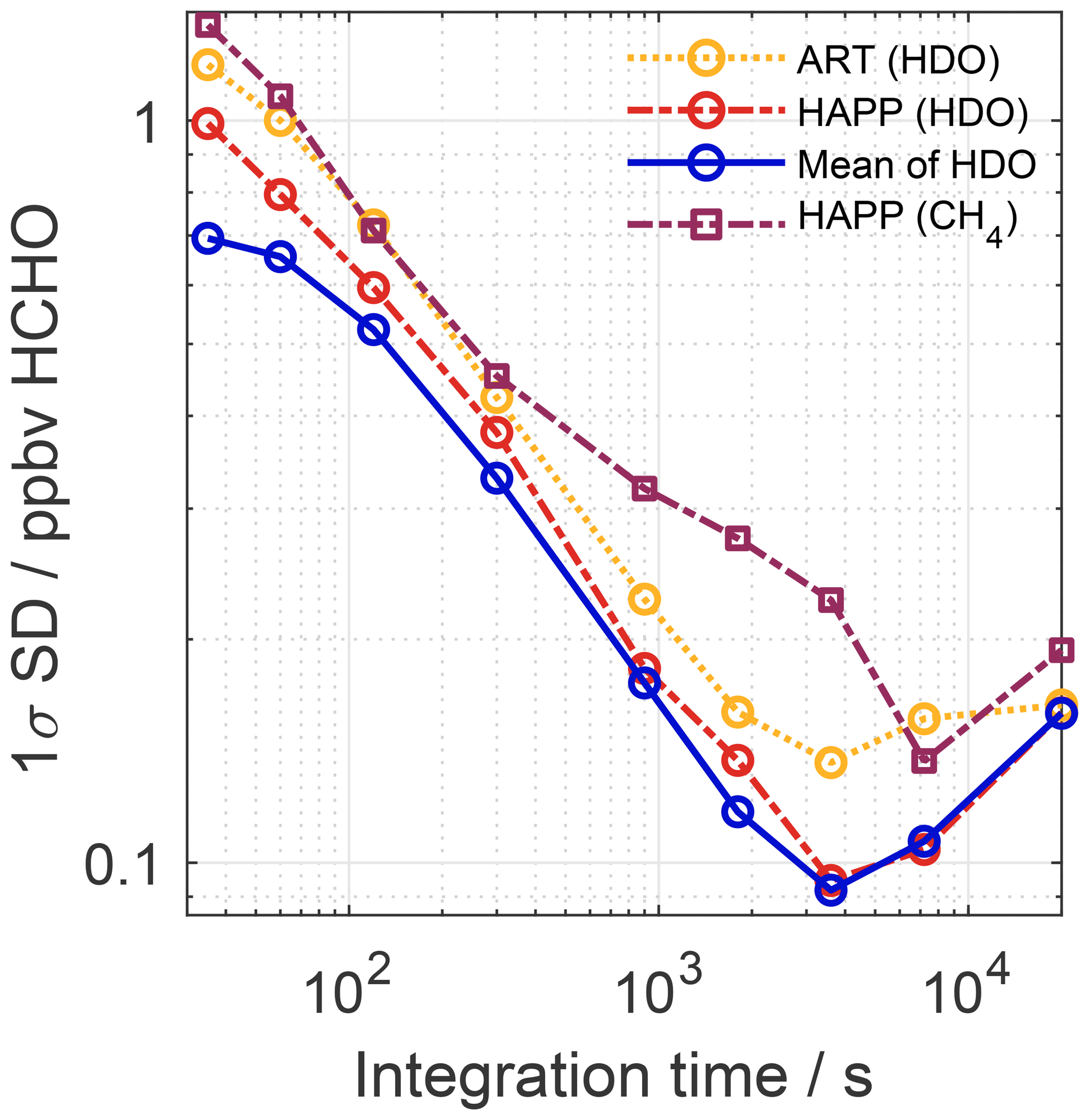
Figure 3Allan–Werle deviation curve HCHO measurements by the Aeris sensor with different fitting modes. In HDO mode, ART and HAPP fits are shown as well as their mean. In CH4 mode, the HAPP fit is shown. The average of the ART and HAPP fits in HDO mode produces the lowest 1σ standard deviation with a minimum of 100 pptv for a 1 h integration time. Table S2 lists 1σ standard deviations at selected integration times and Fig. S2 shows the raw time series data used to derive the Allan–Werle deviation curves.
4.2 Accuracy: LIF intercomparison
To ascertain the linearity and accuracy of the Aeris sensor in both HDO and CH4 modes over HCHO mixing ratios commonly measured in outdoor and indoor locations, the Aeris sensor was compared against several LIF HCHO instruments from both Harvard and NASA. Section 4.2.1 and 4.2.2 show how the Aeris sensor compares with LIF instrumentation in the laboratory (i.e., using HCHO gas standards diluted with ultra-zero air to perform stepped calibrations); conversely, Sect. 4.2.3 shows how the Aeris sensor compares against LIF instrumentation from Harvard when sampling ambient outdoor air over a period of several days.
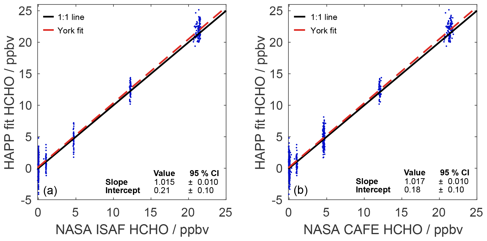
Figure 4Correlation plots between the HAPP HDO fit and two NASA LIF instruments: (a) NASA ISAF (R2=0.979) and (b) NASA CAFE (R2=0.976). A time series plot for the stepped intercomparison performed at NASA Goddard is located in the Supplement (Fig. S4).
The measurement of HCHO by LIF was first applied to in situ atmospheric measurements by Hottle et al. (2009) using a tunable, Ti:sapphire laser. Subsequent work by DiGangi et al. (2011) and Cazorla et al. (2015) replaced the Ti:sapphire laser with a narrow-bandwidth fiber laser. In brief, a fiber laser around 353 nm excites a rotational transition in the vibronic band of HCHO, and a photomultiplier tube (PMT) with a long-pass filter measures the resulting fluorescence at wavelengths longer than 370 nm. The mixing ratio of HCHO is proportional to the laser power-normalized PMT counts. This proportionality constant is determined from a known HCHO standard such as a permeation tube or, more recently, a HCHO gas cylinder (Cazorla et al., 2015).
4.2.1 Stepped calibration with NASA CAFE and ISAF (HDO mode)
During a HCHO multi-hour intercomparison performed at NASA Goddard in November 2017, the Aeris sensor was operated in HDO mode in the laboratory and compared against two NASA LIF instruments: NASA ISAF (In Situ Airborne Formaldehyde; Cazorla et al., 2015) and NASA CAFE (Compact Airborne Formaldehyde Experiment; operating principle described in St. Clair et al., 2017, 2019). Prior to the intercomparison, all instruments were calibrated using HCHO gas cylinder standards that had been verified by Fourier transform infrared (FTIR) spectroscopy. In brief, the HCHO standard is verified by flowing it through an FTIR cell for several hours to allow the signal to equilibrate, and the resulting HCHO mixing ratio is scaled by a factor of 0.957 in order to tie the calibration to UV cross sections by Meller and Moortgat (2000) (Cazorla et al., 2015). During the intercomparison, a HCHO gas cylinder (∼500 ppbv HCHO balance N2; Air Liquide) was diluted by an ultra-zero-air gas cylinder to levels between 0 and 25 ppbv HCHO and flowed into a common sampling manifold. To the inlet line going to the Aeris sensor, an additional flow of 158 sccm of humidified ultra-zero air was added to the total flow of 750 sccm so that the HDO line could be used as a reference. All reported values below from the Aeris sensor have already been corrected for this additional dilution factor.
The ART and HAPP fits were compared for the entirety of the intercomparison. Their relationship is shown (with 95 % confidence intervals computed) in Eq. (2):
In general, the HAPP HDO fit computes mixing ratios that are 2 % lower than those calculated by the ART fit (R2=0.941) along with a negative offset of 150 pptv. A correlation plot between the two HDO fits is shown in Fig. S3.
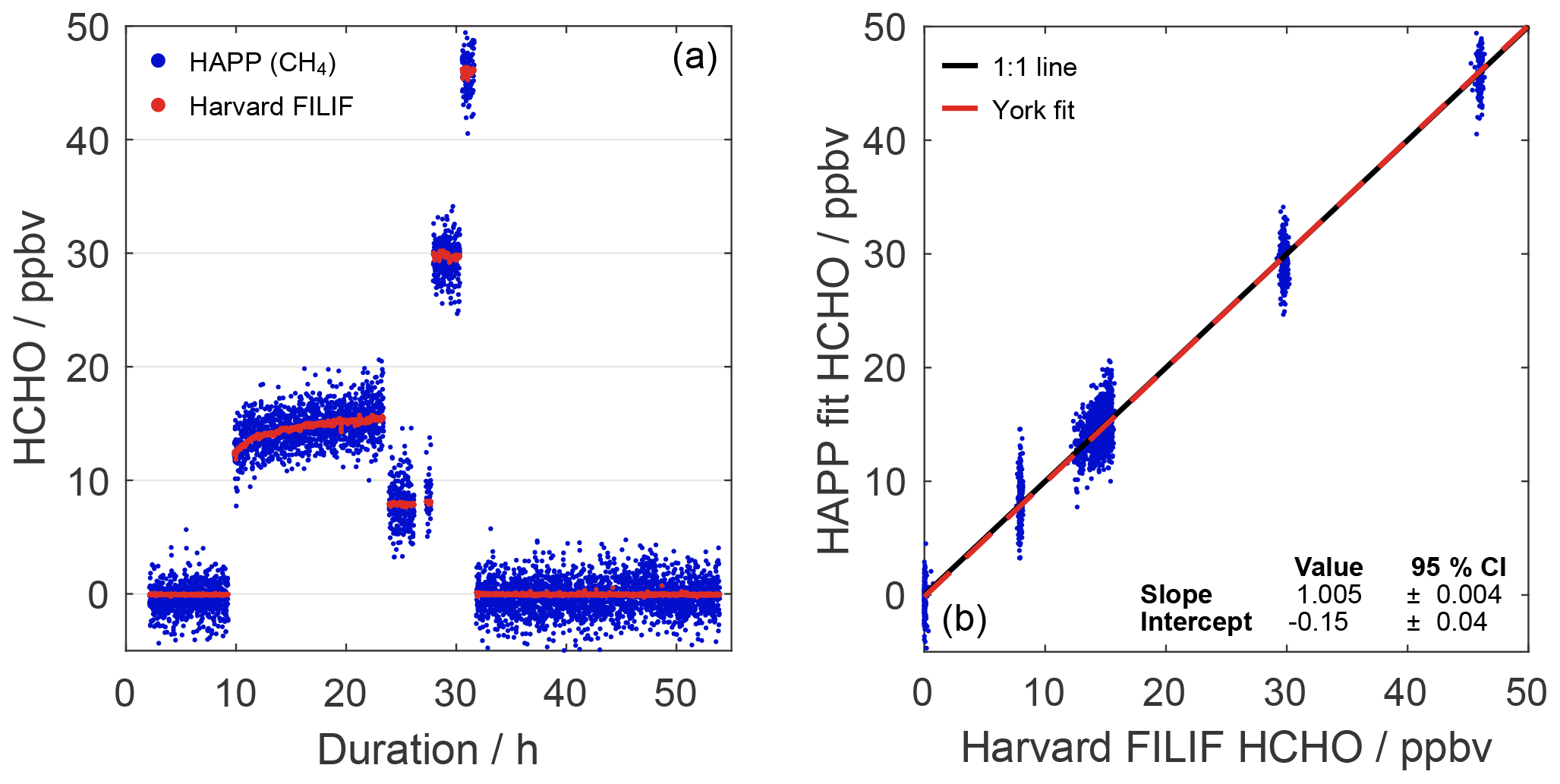
Figure 5(a) Time series of the Aeris sensor (HAPP CH4 fit) and Harvard FILIF during a multiday stepped intercomparison. All data are reported with an integration time of 30 s. (b) Correlation plot between the Aeris sensor (HAPP CH4 fit) and Harvard FILIF (R2=0.980).
Figure 4 shows correlation plots of the HAPP HDO fit versus the NASA ISAF and CAFE instruments, and Fig. S4 shows the time series of these same data with an integration time of 30 s, which is the lowest possible integration time for the Aeris sensor at its default settings. With this integration time, the 1σ standard deviation (using the zero-air segment) of the Aeris sensor was 1000 pptv while those of NASA ISAF and CAFE were 3 and 40 pptv, respectively. Using a bivariate linear regression fit formulated by York et al. (2004), Table 2 shows the relationships between the Aeris sensor and NASA LIF instruments. In both comparisons, the Aeris instrument calculates mixing ratios that are ∼2 % higher than the mixing ratios reported by NASA ISAF or CAFE. The Aeris sensor also displays a slight positive offset of 180 to 210 pptv when compared against the NASA instrumentation.
Table 2Regression analyses for Aeris sensor vs. LIF instruments under laboratory conditions calculated with a 95 % confidence interval.
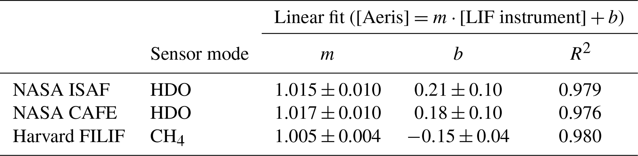
Bivariate least-squares regressions were calculated according to the method of York et al. (2004). HAPP fits were used for reporting the HCHO mixing ratio from the Aeris sensor. Laboratory conditions denote diluting HCHO gas standards using ultra-zero air. Units are in parts per billion by volume.
4.2.2 Stepped calibration with Harvard FILIF (CH4 mode)
The Aeris sensor was also operated in CH4 mode in the laboratory and compared against the Harvard FILIF (fiber-laser-induced fluorescence) HCHO instrument described previously (DiGangi et al., 2011; Hottle et al., 2009) but with several modifications which will be briefly outlined. First, the 32-pass White-type multi-pass detection cell has been replaced with a more stable and easier-to-align single-pass detection cell as described and used in Cazorla et al. (2015). The single-pass cell is coated in an ultra-black carbon nanotube coating (Singularity Black; NanoLab, Inc.) that minimizes noise in the photomultiplier tube due to scattered photons from the 353 nm laser (NovaWave Technologies, Inc., TFL series). Upgrades to the instrument's electronics and software (now running QNX) have also been performed to increase its reliability as it samples at a default rate of 10 Hz.
This intercomparison utilized a HCHO gas cylinder (600 ppbv HCHO balance N2; Air Liquide) that was diluted with ultra-zero air (Airgas) to levels between 0 and 50 ppbv HCHO and flowed into a common sampling line. A check of the mixing ratio of HCHO in the calibration tank by FTIR showed that the scaled FTIR-derived mixing ratio (524±15 ppbv HCHO) was 13 % less than what was quoted on the tank, so the scaled FTIR-derived value was used for this comparison. To the 5000 sccm gas flow from the ultra-zero-air tank, < 1 sccm of ultrapure CH4 (chemically pure 99.5 % methane; Airgas) was added so that the Aeris sensor was running in CH4 mode.
Figure 5 shows the results of the multiday stepped intercomparison between Harvard FILIF and the Aeris sensor. In the first nonzero HCHO step, both the Aeris sensor and Harvard FILIF instrument show that the HCHO mixing ratio took several hours to stabilize at 15.3 ppbv. This is likely due to the HCHO gas passivating the stainless-steel surfaces of the gas regulator and MKS Instruments mass flow controller (500 sccm full scale) even though the latter was coated in a FluoroPel omniphobic coating (FluoroPel 800; Cytonix). All other surfaces were PFA plastic. This highlights the need to perform HCHO calibrations over several hours to allow for passivation of all surfaces.
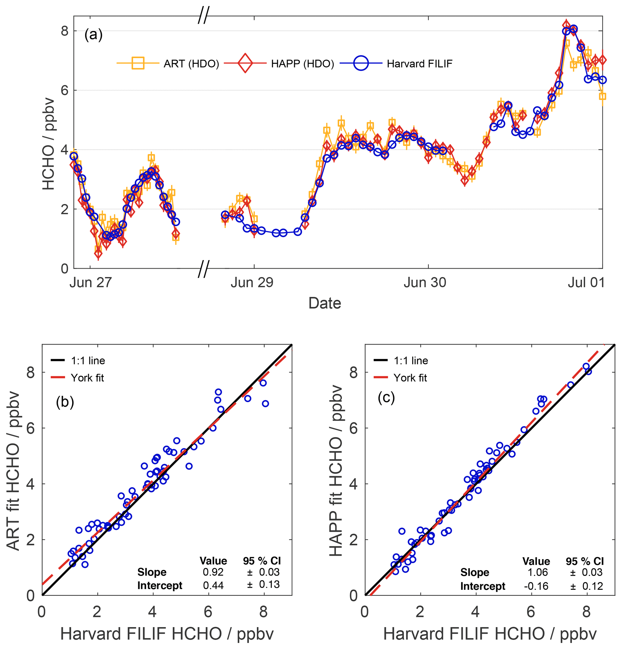
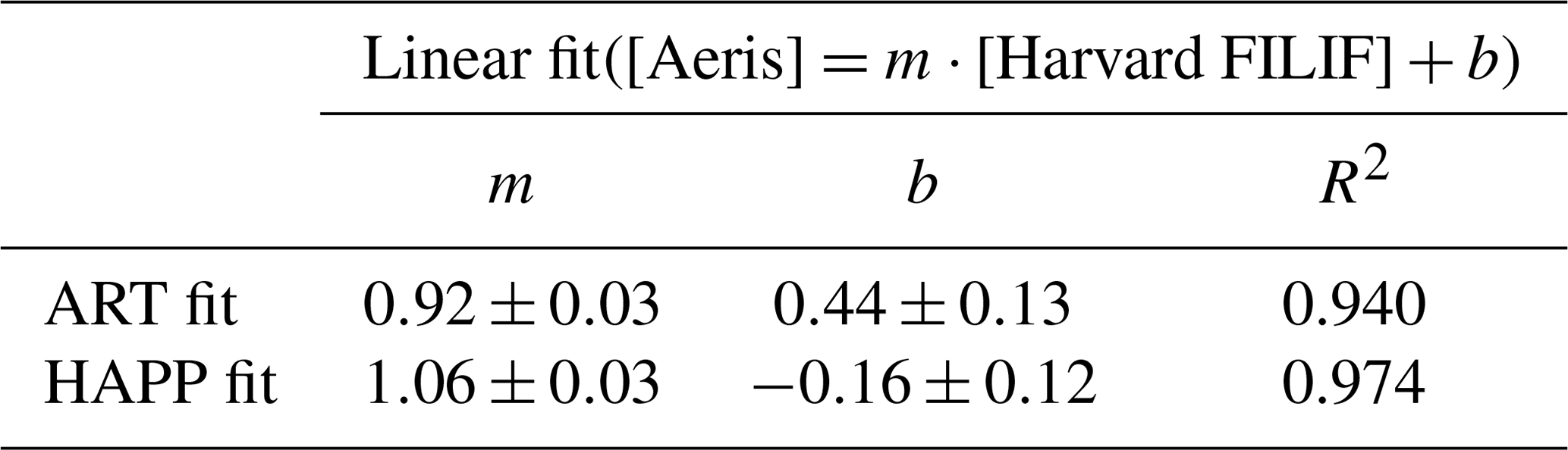
Figure 6(a) Collocated, multiday sampling of ambient air in Cambridge, MA, by Harvard FILIF and the Aeris sensor (HDO mode). Ticks represent midnight (00:00) on the specified date. All data are reported with an integration time of 60 min. From the evenings of 27 to 28 June, the area experienced rain showers that caused both the ART and HAPP fits to underestimate the HCHO mixing ratio by ∼0.5 ppbv due to water condensing on the optics. Data from the Aeris sensor were also removed (1) during the early hours of 29 June due to replacement of the DNPH cartridge and (2) during the afternoon of 30 June due to zeroing of the sensor with ultra-zero air. Correlation plots comparing Harvard FILIF with (b) ART fit (R2=0.940) and (c) HAPP fit (R2=0.974).
At 30 s, the Aeris sensor had a 1σ precision of 1350 pptv as opposed to 22 pptv for Harvard FILIF during this experiment. The difference does improve at a 1 h integration time when the 1σ precision for the Aeris becomes 230 pptv and that of FILIF is 8.5 pptv. Table 2 shows the results of a linear regression of the HCHO mixing ratios from the Aeris sensor versus those reported by Harvard FILIF. The regression shows the Aeris sensor reporting the HCHO mixing ratio as ∼1 % higher when compared to FILIF with a negative offset of 150 pptv. These results obtained with a different calibration tank and different LIF instrument are in excellent agreement with the ones obtained during the intercomparison at NASA Goddard, demonstrating the Aeris sensor's accuracy and linearity even at low mixing ratios.
4.2.3 Ambient air intercomparison with Harvard FILIF (HDO mode)
In order to ascertain the performance of the Aeris sensor when sampling ambient air, the sensor and Harvard FILIF were collocated in Cambridge, MA, to sample outdoor air for several days at the end of June 2018 (both instruments used the same inlet line). The ART and HAPP fit hourly averages for HCHO in HDO mode are compared against the mixing ratios from Harvard FILIF in Fig. 6. Though conditions during the measurement period were generally partly or mostly cloudy with highs reaching 33 ∘C by the end of the week, it was punctuated by rain showers that lasted from the evening of 27 June to the evening of 28 June. During this time, both ART and HAPP fit HCHO underpredicted FILIF by ∼500 pptv, though this is a sampling error due to water condensing onto the optics of the sensor (as evidenced by some slight water damage observed on the optical coating following this experiment). This problem can be alleviated in the future with an inline water trap and ensuring that the sensor is not substantially colder than the temperature of the ambient air.
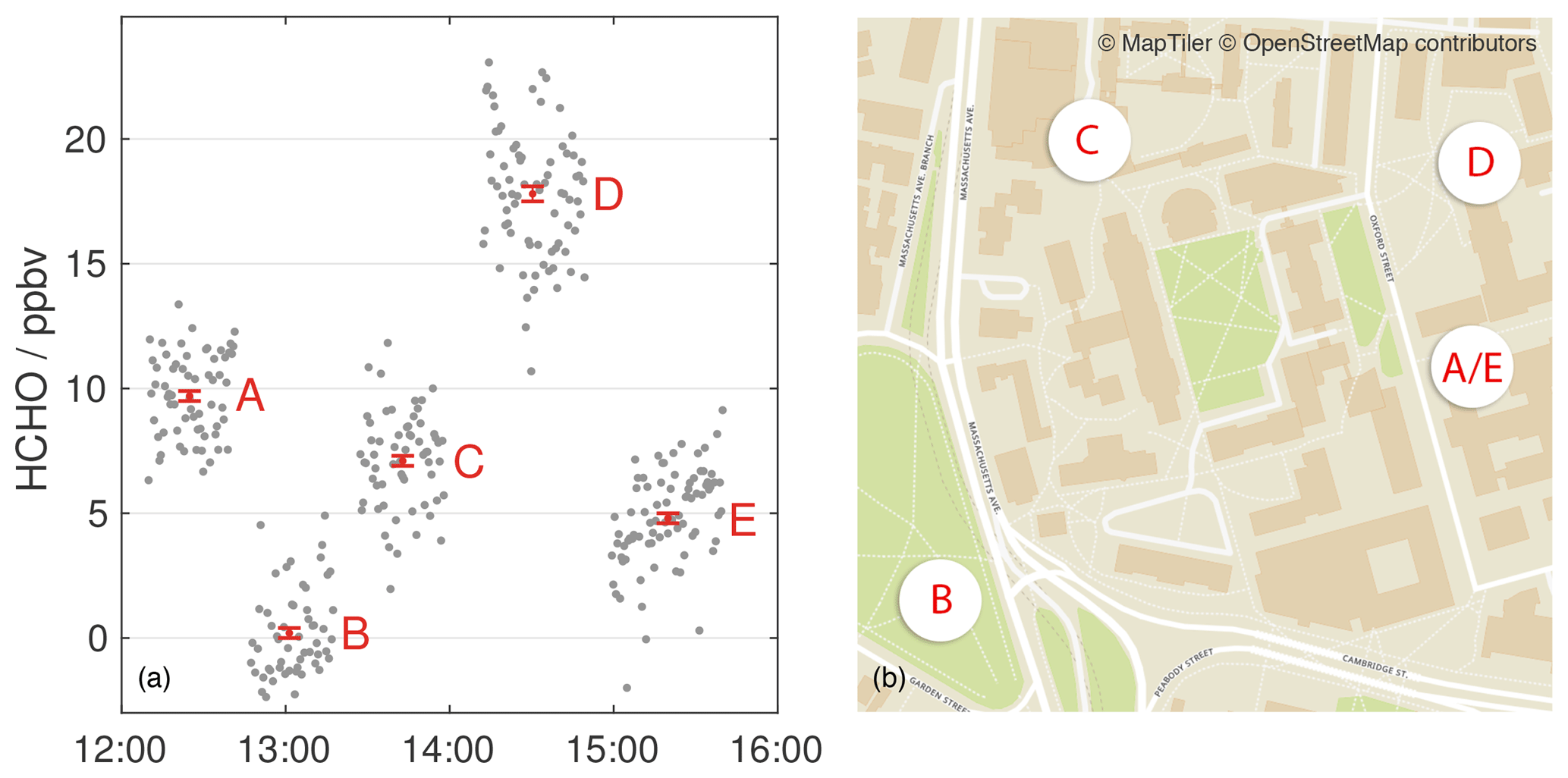
Figure 7(a) Aeris sensor (operating in HAPP fit HDO mode) used as a HCHO personal exposure monitor for several hours on a single battery charge around the Harvard campus in Cambridge, MA. All times EDT. Locations included (A) office space (N=64 points), (B) urban park (N=55 points), (C) cafeteria (N=62 points), (D) museum space (N=75 points), and (E) lab space (N=82 points). The data from HAPP fit is displayed with the raw 30 s data (grey) as well as the average and ±1σ standard deviation of the mean for each location (red). Data is not shown when the sensor was transported from one location to another. (b) Map data © OpenStreetMap contributors. Schema from OpenMapTiles.org (MapTiler and OpenStreetMap Contributors, 2018).
Considering all hours except for the rain showers (n=63 h), 87 % of the HAPP fit hourly mixing ratios are within ±0.5 ppbv of FILIF and 100 % are within ±1 ppbv. Similarly, 73 % and 98 % of the ART fit hourly mixing ratios are within ±0.5 and ±1 ppbv of FILIF, respectively. Table 3 shows the results of a linear regression of ART and HAPP fit HCHO mixing ratios versus those reported by FILIF. The regression demonstrates that the ART fit mixing ratios were ∼8 % lower than FILIF with a positive offset of 440 pptv. Conversely, the HAPP fit mixing ratios were ∼6 % higher than FILIF with a negative offset of 160 pptv. With both fits within ±10 % of FILIF, these results readily demonstrate the utility of using the Aeris sensor as a monitor for ambient levels of HCHO in the environment.
Table 3Regression analysis for Aeris sensor vs. Harvard FILIF sampling ambient air calculated with a 95 % confidence interval.
Bivariate least-squares regressions were calculated according to the method of York et al. (2004). Units are in parts per billion by volume.
In determining the sensor's accuracy, there is a clear difference between how well the Aeris sensor compared to LIF instrumentation under laboratory conditions (i.e., HCHO gas standards diluted by ultra-zero air to perform stepped calibrations) (Table 2) and when sampling ambient air (Table 3). From the stepped calibrations performed in Sect. 4.2.1 and 4.2.2., the mean HCHO mixing ratio at each step reported by HAPP fit was generally within ±4 % of the mean value reported by LIF instrumentation. During the ambient air intercomparison with Harvard FILIF, both ART and HAPP fit showed that they were within −8 % and +6 %, respectively, when compared to LIF. Taking into account the 95 % confidence intervals derived from the York fits in Table 3 and a maximum offset of ∼0.3 ppbv during LIF intercomparison under laboratory conditions, an accuracy of ± (10 % + 0.3) ppbv should be quoted for the Aeris sensor. The factor that affects the accuracy of the Aeris sensor the most likely stems from any instabilities and movements in fringes caused by the optical train's etalons (perhaps from temperature fluctuations) since any drift can subsequently impact how well the HCHO line is fit. Other matrix effects impacting the sensor's accuracy include particles that happen to pass through the inline filter and scatter the laser light as well as minor gas-phase absorbers not listed in the HITRAN database.
One of the advantages of the Aeris sensor over other instruments is its light weight and portability, so a demonstration of the portability of the Aeris sensor was performed by carrying it around as a personal HCHO exposure monitor around the Harvard campus. Figure 7 shows a map of the locations visited. Even though the data were collected during a winter month in Massachusetts when the air is generally cold and dry (which would necessitate running in CH4 mode), the sensor operated in HDO mode due to an unseasonal local temperature of 22 ∘C and 63 % relative humidity. The sensor's batteries did not have to be recharged during the measurement period.
The five measurement sites (HAPP HDO fit HCHO mixing ratios and ±1σ standard deviation of the mean for each location in parentheses) were (A) an office space (9.7±0.2 ppbv), (B) an urban park (0.2±0.2 ppbv), (C) a cafeteria during lunchtime (7.1±0.2 ppbv), (D) the ant collection room in the Harvard Natural History Museum (17.8±0.3 ppbv), and (E) laboratory space in the Mallinckrodt Chemistry Lab (4.8±0.2 ppbv). All locations were indoors except for B. This sampling demonstrates the portability of the sensor in both indoor and outdoor locations and its potential use in indoor air chemistry studies. Even though the LIF instruments have much higher precision than the Aeris sensor, this simple experiment around the Harvard campus would have been cumbersome and logistically impractical given the size and power requirements of the LIF instruments and other spectroscopic and spectrometric methods mentioned previously. Moreover, all the mixing ratios were calculated in real time unlike offline HCHO measurement methods such as the current EPA standard methodology.
While the Aeris sensor is not a replacement for research-grade instrumentation for measuring HCHO in some applications, its ease of use, portability, and cost make the sensor a prime candidate for use in a variety of routine monitoring applications. The 3σ limit of detection at a 15 min integration time is 690 and 570 pptv HCHO for ART and HAPP fits, respectively, which improves to 420 and 300 pptv HCHO at a 60 min integration time. With sub-parts-per-billion-by-volume precision at these times, the sensor can easily distinguish between ambient levels of HCHO normally found in outdoor and indoor locations. Moreover, the ambient outdoor air intercomparison with Harvard FILIF in Fig. 6 shows that the Aeris sensor hourly HCHO is generally within ±0.5 ppbv of the HCHO mixing ratio reported by LIF instrumentation. This intercomparison demonstrates that the sensor is a viable alternative for ambient air monitoring networks or perhaps indoor air chemistry studies.
As discussed in the text, the sensor can operate in both HDO and CH4 modes. While HDO mode is preferable in most cases, during cold weather operation when the air is dry, it is recommended to run the Aeris sensor in CH4 mode by adding a < 1 sccm flow from an ultrapure CH4 gas tank. While this makes the sensor less portable, it ensures that data can still be collected in these conditions. The need for a spare CH4 gas tank would be made obsolete if a small CH4 reference cell were added to the sensor or the etalons were reduced or better characterized by software to improve the signal-to-noise ratio on the HDO spectral line.
HAPP fit can be provided upon request by email to Norton T. Allen (allen@huarp.harvard.edu). Data used in this paper can be provided upon request by email to Joshua D. Shutter (shutter@g.harvard.edu).
The supplement related to this article is available online at: https://doi.org/10.5194/amt-12-6079-2019-supplement.
JDS led this work, designed and carried out experiments, completed the data analysis, and wrote the paper with input from all co-authors. NTA wrote HAPP fit and assisted JDS with data analysis. TFH oversees all NASA LIF instrumentation and approved intercomparison efforts at NASA Goddard. GMW provided data from NASA ISAF and designed experiments during the NASA Goddard intercomparison in November–December 2017. JMSC provided data from NASA CAFE. As principal investigator, FNK provided supervision and acquired financial support for this project.
The authors declare that they have no conflict of interest.
The authors acknowledge Aeris Technologies (Joshua B. Paul, Jerome Thiebaud, Stephen So, and James J. Scherer) for helpful discussions along with the development and fabrication of the sensor. Additionally, the authors acknowledge Joshua L. Cox for his assistance during the HCHO intercomparison at NASA Goddard in November–December 2017.
This research has been supported by the National Science Foundation Graduate Research Fellowship (grant no. DGE–1745303).
This paper was edited by Keding Lu and reviewed by three anonymous referees.
Anderson, L. G., Lanning, J. A., Barrell, R., Miyagishima, J., Jones, R. H., and Wolfe, P.: Sources and sinks of formaldehyde and acetaldehyde: An analysis of Denver's ambient concentration data, Atmos. Environ., 30, 2113–2123, https://doi.org/10.1016/1352-2310(95)00175-1, 1996.
Baucus, M.: S. 1630 – 101st Congress: Clean Air Act Amendments of 1990, United States Congress, Washington, DC, 1990.
Cazorla, M., Wolfe, G. M., Bailey, S. A., Swanson, A. K., Arkinson, H. L., and Hanisco, T. F.: A new airborne laser-induced fluorescence instrument for in situ detection of formaldehyde throughout the troposphere and lower stratosphere, Atmos. Meas. Tech., 8, 541–552, https://doi.org/10.5194/amt-8-541-2015, 2015.
Centers for Disease Control and Prevention: NIOSH Pocket Guide to Chemical Hazards, available at: https://www.cdc.gov/niosh/npg/npgd0293.html (last access: 30 September 2018), 2007.
Chan Miller, C., Jacob, D. J., Marais, E. A., Yu, K., Travis, K. R., Kim, P. S., Fisher, J. A., Zhu, L., Wolfe, G. M., Hanisco, T. F., Keutsch, F. N., Kaiser, J., Min, K.-E., Brown, S. S., Washenfelder, R. A., González Abad, G., and Chance, K.: Glyoxal yield from isoprene oxidation and relation to formaldehyde: chemical mechanism, constraints from SENEX aircraft observations, and interpretation of OMI satellite data, Atmos. Chem. Phys., 17, 8725–8738, https://doi.org/10.5194/acp-17-8725-2017, 2017.
Choi, W., Faloona, I. C., Bouvier-Brown, N. C., McKay, M., Goldstein, A. H., Mao, J., Brune, W. H., LaFranchi, B. W., Cohen, R. C., Wolfe, G. M., Thornton, J. A., Sonnenfroh, D. M., and Millet, D. B.: Observations of elevated formaldehyde over a forest canopy suggest missing sources from rapid oxidation of arboreal hydrocarbons, Atmos. Chem. Phys., 10, 8761–8781, https://doi.org/10.5194/acp-10-8761-2010, 2010.
DiGangi, J. P., Boyle, E. S., Karl, T., Harley, P., Turnipseed, A., Kim, S., Cantrell, C., Maudlin III, R. L., Zheng, W., Flocke, F., Hall, S. R., Ullmann, K., Nakashima, Y., Paul, J. B., Wolfe, G. M., Desai, A. R., Kajii, Y., Guenther, A., and Keutsch, F. N.: First direct measurements of formaldehyde flux via eddy covariance: implications for missing in-canopy formaldehyde sources, Atmos. Chem. Phys., 11, 10565–10578, https://doi.org/10.5194/acp-11-10565-2011, 2011.
Fried, A., Wert, B. P., Henry, B., and Drummond, J. R.: Airborne tunable diode laser measurements of formaldehyde, Spectrochim. Acta A Mol. Biomol. Spectrosc., 55, 2097–2110, https://doi.org/10.1016/S1386-1425(99)00082-7, 1999.
Gordon, I. E., Rothman, L. S., Hill, C., Kochanov, R. V., Tan, Y., Bernath, P. F., Birk, M., Boudon, V., Campargue, A., Chance, K. V., Drouin, B. J., Flaud, J.-M., Gamache, R. R., Hodges, J. T., Jacquemart, D., Perevalov, V. I., Perrin, A., Shine, K. P., Smith, M.-A. H., Tennyson, J., Toon, G. C., Tran, H., Tyuterev, V. G., Barbe, A., Császár, A. G., Devi, V. M., Furtenbacher, T., Harrison, J. J., Hartmann, J.-M., Jolly, A., Johnson, T. J., Karman, T., Kleiner, I., Kyuberis, A. A., Loos, J., Lyulin, O. M., Massie, S. T., Mikhailenko, S. N., Moazzen-Ahmadi, N., Müller, H. S. P., Naumenko, O. V., Nikitin, A. V., Polyansky, O. L., Rey, M., Rotger, M., Sharpe, S. W., Sung, K., Starikova, E., Tashkun, S. A., Vander Auwera, J., Wagner, G., Wilzewski, J., Wcisło, P., Yu, S., and Zak, E. J.: The HITRAN2016 molecular spectroscopic database, J. Quant. Spectrosc. Ra., 203, 3–69, https://doi.org/10.1016/J.JQSRT.2017.06.038, 2017.
Holzinger, R., Warneke, C., Hansel, A., Jordan, A., Lindinger, W., Scharffe, D. H., Schade, G., and Crutzen, P. J.: Biomass burning as a source of formaldehyde, acetaldehyde, methanol, acetone, acetonitrile, and hydrogen cyanide, Geophys. Res. Lett., 26, 1161–1164, https://doi.org/10.1029/1999GL900156, 1999.
Hottle, J. R., Huisman, A. J., DiGangi, J. P., Kammrath, A., Galloway, M. M., Coens, K. L., and Keutsch, F. N.: A laser induced fluorescence-based instrument for in-situ measurements of atmospheric formaldehyde, Environ. Sci. Technol., 43, 790–795, https://doi.org/10.1021/es801621f, 2009.
Kaiser, J., Li, X., Tillmann, R., Acir, I., Holland, F., Rohrer, F., Wegener, R., and Keutsch, F. N.: Intercomparison of Hantzsch and fiber-laser-induced-fluorescence formaldehyde measurements, Atmos. Meas. Tech., 7, 1571–1580, https://doi.org/10.5194/amt-7-1571-2014, 2014.
Klepeis, N. E., Nelson, W. C., Ott, W. R., Robinson, J. P., Tsang, A. M., Switzer, P., Behar, J. V., Hern, S. C., and Engelmann, W. H.: The National Human Activity Pattern Survey (NHAPS): A resource for assessing exposure to environmental pollutants, J. Expo. Sci. Environ. Epidemiol., 11, 231–252, https://doi.org/10.1038/sj.jea.7500165, 2001.
MapTiler and OpenStreetMap Contributors: Maputnik v1.5.0, OpenStreetMap data is available under the Open Database License and cartography is licensed as CC BY-SA, available at: https://www.openstreetmap.org, https://openmaptiles.org, and https://maputnik.github.io (last access: 1 August 2018), 2018.
McManus, J. B., Zahniser, M. S., Nelson, D. D., Shorter, J. H., Herndon, S. C., Wood, E. C., and Wehr, R.: Application of quantum cascade lasers to high-precision atmospheric trace gas measurements, Opt. Eng., 49, 111124, https://doi.org/10.1117/1.3498782, 2010.
Meller, R. and Moortgat, G. K.: Temperature dependence of the absorption cross sections of formaldehyde between 223 and 323 K in the wavelength range 225–375 nm, J. Geophys. Res.-Atmos., 105, 7089–7101, https://doi.org/10.1029/1999JD901074, 2000.
Nazaroff, W. W. and Weschler, C. J.: Cleaning products and air fresheners: Exposure to primary and secondary air pollutants, Atmos. Environ., 38, 2841–2865, https://doi.org/10.1016/J.ATMOSENV.2004.02.040, 2004.
Paul, J. B.: Compact Folded Optical Multipass System, US Patent #10,222,595, 2019.
Rothman, L. S., Gordon, I. E., Babikov, Y., Barbe, A., Benner, D. C., Bernath, P. F., Birk, M., Bizzocchi, L., Boudon, V., Brown, L. R., Campargue, A., Chance, K., Cohen, E. A., Coudert, L. H., Devi, V. M., Drouin, B. J., Fayt, A., Flaud, J.-M., Gamache, R. R., Harrison, J. J., Hartmann, J.-M., Hill, C., Hodges, J. T., Jacquemart, D., Jolly, A., Lamouroux, J., Le Roy, R. J., Li, G., Long, D. A., Lyulin, O. M., Mackie, C. J., Massie, S. T., Mikhailenko, S., Müller, H. S. P., Naumenko, O. V., Nikitin, A. V., Orphal, J., Perevalov, V., Perrin, A., Polovtseva, E. R., Richard, C., Smith, M. A. H., Starikova, E., Sung, K., Tashkun, S., Tennyson, J., Toon, G. C., Tyuterev, Vl. G., and Wagner, G.: The HITRAN2012 molecular spectroscopic database, J. Quant. Spectrosc. Ra., 130, 4–50, https://doi.org/10.1016/j.jqsrt.2013.07.002, 2013.
Salthammer, T.: Formaldehyde in the ambient atmosphere: From an indoor pollutant to an outdoor pollutant?, Angew. Chemie Int. Ed., 52, 3320–3327, https://doi.org/10.1002/anie.201205984, 2013.
Sayres, D. S., Moyer, E. J., Hanisco, T. F., St Clair, J. M., Keutsch, F. N., O'Brien, A., Allen, N. T., Lapson, L., Demusz, J. N., Rivero, M., Martin, T., Greenberg, M., Tuozzolo, C., Engel, G. S., Kroll, J. H., Paul, J. B., and Anderson, J. G.: A new cavity based absorption instrument for detection of water isotopologues in the upper troposphere and lower stratosphere, Rev. Sci. Instrum., 80, 044102, https://doi.org/10.1063/1.3117349, 2009.
Seinfeld, J. H. and Pandis, S. N.: Atmospheric Chemistry and Physics: From Air Pollution to Climate Change, 3rd edn., Wiley, Hoboken, New Jersey, 2016.
St. Clair, J. M., Swanson, A. K., Bailey, S. A., Wolfe, G. M., Marrero, J. E., Iraci, L. T., Hagopian, J. G., and Hanisco, T. F.: A new non-resonant laser-induced fluorescence instrument for the airborne in situ measurement of formaldehyde, Atmos. Meas. Tech., 10, 4833–4844, https://doi.org/10.5194/amt-10-4833-2017, 2017.
St. Clair, J. M., Swanson, A. K., Bailey, S. A., and Hanisco, T. F.: CAFE: a new, improved nonresonant laser-induced fluorescence instrument for airborne in situ measurement of formaldehyde, Atmos. Meas. Tech., 12, 4581–4590, https://doi.org/10.5194/amt-12-4581-2019, 2019.
U.S. Environmental Protection Agency: Risk Assessment for Carcinogenic Effects, available at: https://www.epa.gov/fera/risk-assessment-carcinogenic-effects (last access: 16 August 2018), 2018.
Vlasenko, A., Macdonald, A. M., Sjostedt, S. J., and Abbatt, J. P. D.: Formaldehyde measurements by Proton transfer reaction – Mass Spectrometry (PTR-MS): correction for humidity effects, Atmos. Meas. Tech., 3, 1055–1062, https://doi.org/10.5194/amt-3-1055-2010, 2010.
Washenfelder, R. A., Attwood, A. R., Flores, J. M., Zarzana, K. J., Rudich, Y., and Brown, S. S.: Broadband cavity-enhanced absorption spectroscopy in the ultraviolet spectral region for measurements of nitrogen dioxide and formaldehyde, Atmos. Meas. Tech., 9, 41–52, https://doi.org/10.5194/amt-9-41-2016, 2016.
Weibring, P., Richter, D., Walega, J. G., and Fried, A.: First demonstration of a high performance difference frequency spectrometer on airborne platforms, Opt. Express, 15, 13476–13495, https://doi.org/10.1364/OE.15.013476, 2007.
Winberry, W. T., Tejada, S., Lonneman, B., and Kleindienst, T.: Compendium of Methods for the Determination of Toxic Organic Compounds in Ambient Air: Compendium Method TO-11A, 2nd edn., U.S. Environmental Protection Agency, Cincinnati, OH, 1999.
Wisthaler, A., Apel, E. C., Bossmeyer, J., Hansel, A., Junkermann, W., Koppmann, R., Meier, R., Müller, K., Solomon, S. J., Steinbrecher, R., Tillmann, R., and Brauers, T.: Technical Note: Intercomparison of formaldehyde measurements at the atmosphere simulation chamber SAPHIR, Atmos. Chem. Phys., 8, 2189–2200, https://doi.org/10.5194/acp-8-2189-2008, 2008.
York, D., Evensen, N. M., Martínez, M. L., and De Basabe Delgado, J.: Unified equations for the slope, intercept, and standard errors of the best straight line, Am. J. Phys., 72, 367–375, https://doi.org/10.1119/1.1632486, 2004.
Zhu, L., Jacob, D. J., Keutsch, F. N., Mickley, L. J., Scheffe, R., Strum, M., González Abad, G., Chance, K., Yang, K., Rappenglück, B., Millet, D. B., Baasandorj, M., Jaeglé, L., and Shah, V.: Formaldehyde (HCHO) as a hazardous air pollutant: Mapping surface air concentrations from satellite and inferring cancer risks in the United States, Environ. Sci. Technol., 51, 5650–5657, https://doi.org/10.1021/acs.est.7b01356, 2017a.
Zhu, L., Mickley, L. J., Jacob, D. J., Marais, E. A., Sheng, J., Hu, L., Abad, G. G., and Chance, K.: Long-term (2005–2014) trends in formaldehyde (HCHO) columns across North America as seen by the OMI satellite instrument: Evidence of changing emissions of volatile organic compounds, Geophys. Res. Lett., 44, 7079–7086, https://doi.org/10.1002/2017GL073859, 2017b.
- Abstract
- Introduction
- Instrument description
- Data processing: Harvard Aeris Post-Processing (HAPP) fit
- Sensor characterization
- Portability demonstration
- Conclusions
- Code and data availability
- Author contributions
- Competing interests
- Acknowledgements
- Financial support
- Review statement
- References
- Supplement