2.1 Assembly and optical setup

For ease of reading, the following section defines a common coordinate system for Figs. 1–4. Furthermore, we define a common set of identifiers, where alphanumeric labelling is used to identify physical parts and roman numerals are used to identify scenarios or alternative views (within the coordinate system). The structural components of the UCASS, shown in Fig. 1, are made primarily from 3-D printed parts. The design is essentially tubular, 180 mm long and 64 mm in diameter. An elliptical cross section hole, 30 mm × 22 mm in size, runs the full length of the UCASS body and offers a low impedance path for the sample flow, defined as the −y direction in the instrument coordinate system. The UCASS is designed with this particular shape for use as a dropsonde system, whereby a connected KITsonde fits inside the UCASS and the entire payload fits within a standard release container. This is discussed further in Sect. 3.2.1. The main unit (a1) is 3-D printed from nylon using selective laser sintering (SLS). This process is chosen for the main unit as it produces a mechanically rigid and thermally stable chassis, which is crucial for the instrument to endure the temperature cycle associated with a routine sounding. The process uses a layer thickness of 0.12 mm, which is adequate for the placement of mechanical components such as batteries and circuitry. However, to improve the precision for optical components, a modular design is used, thus allowing each optical element to be aligned and secured individually. The beam-forming optics are mounted onto an insert (a2), which is 3-D printed from polylactic acid (PLA) using fused filament fabrication (FFF). This method is chosen for increased mechanical rigidity, which is required for the thin wall thicknesses. The elliptical mirror is mounted on an aluminium insert (a3), which is machined using a five-axis mill. Once the beam-forming optics are aligned, the insert (a2) is secured into place in the main unit. The elliptical mirror, mounted on insert (a3) is aligned using three adjustment screws, which secure the mirror onto the main unit (a1). Once assembled, the UCASS is enclosed by a 3-D printed sleeve (a4) and (a5).

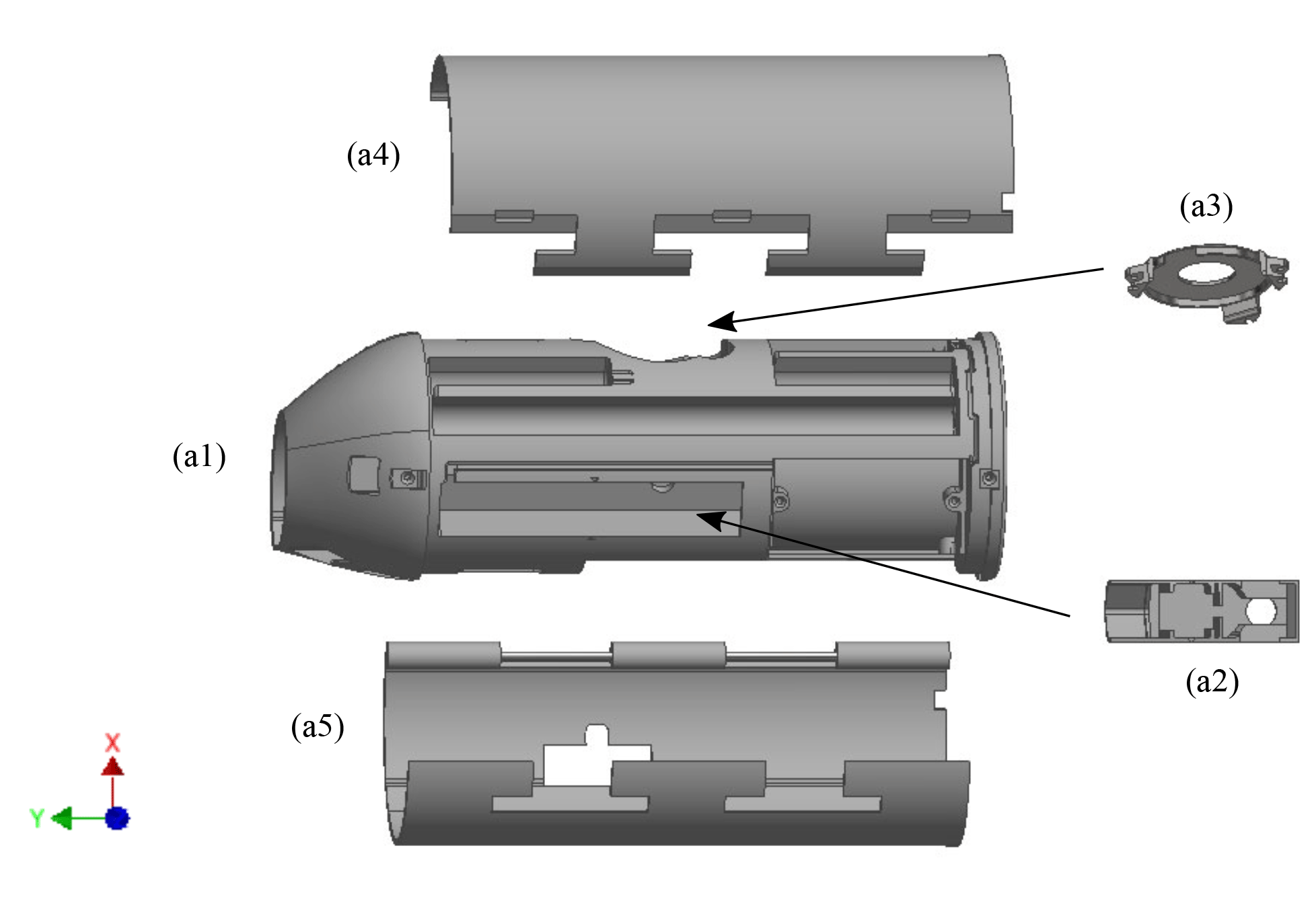
Figure 1Structural components of the UCASS. This consists of four 3-D printed components: the main housing unit (a1), inserts for the beam-forming optics (a2) and the outer casing (a4) and (a5). The mirror holder (a3) is machined out of aluminium.

Download

The optical assembly is shown in Fig. 2. Here, the UCASS chassis (a1) is shown as a transparent layer to illustrate the placement of the optical elements. Figure 2a shows a view along the x–y plane (parallel to the airflow), and Fig. 2b shows a view in the x–z plane (perpendicular to the airflow). The input beam is a 658 nm continuous-wave diode laser (b1) from Oclaro (part no. HL6501MG), operating at 10 mW. The laser is fitted with a collimator from the Optoelectronics Company (part no. 500-020012). The collimated beam of the elliptical cross section is approximately 3.5 mm (long axis) by 2 mm (short axis) and is focused along the short axis by a 50 mm focal length cylindrical lens (b2) from Edmund Optics (part no. 68-047) and then passes through a 2 mm aperture (b3) perpendicular to the beam's long axis. For ease of assembly, these beam-forming components (parts b1, b2 and b3 in Fig. 2) are mounted onto an insert (part a2 in Fig. 1). A plane 9 mm × 9 mm front silvered mirror (b4) from Edmund optics (part no. 31-004) reflects the beam at 45^∘, directing it across the flow of air through the UCASS body, it is then extinguished within the UCASS casing via a cavity coated with absorptive paint. The input beam is shown in red in Fig. 2. The 2 mm aperture has the effect of reforming the beam's Gaussian intensity profile into an approximate “top hat” profile such that, at the sensing area (coincident with the focal distance of the cylindrical lens), the beam has a relatively uniform intensity cross section of ≈2 mm width by ≈40 µm depth. Particles passing through the beam parallel to its short axis therefore experience similar levels of irradiance, a prerequisite for accurate particle sizing. This is discussed in Sect. 2.2.

Particles carried in the airflow through the UCASS may pass through the laser at any point in its traversal across the air flow path. However, only those passing through a specific 0.5 mm² sensing area within the laser beam are measured. This sensing area is defined optically by a custom-designed combination of concave elliptical mirror (b5) and a dual-area photodiode detector (b6). Both mirror and detector were designed by the University of Hertfordshire and are now commercially produced by Alphasense Ltd (part no. 836-0001-00) and First Sensor GmbH (part no. DP12.5-6 SMD), respectively, available only through special order. The elliptical mirror (b5) collects light scattered by a particle passing through the sensing area of the laser beam into a solid angle element of 1.69 sr (scattering angles from 16 to 104^∘) and directs it towards the photodiode detector (b6), where the total intensity is measured.

Figure 2Optical assembly of the UCASS. Panel (a) shows a view in the x–y plane, parallel to the airflow. Panel (b) shows a view in the x–z plane, perpendicular to the airflow. The beam-forming optics consist of a laser with collimator (b1), a cylindrical lens (b2) and a 2 mm aperture (b3). The beam is directed into the instrument via a front silvered mirror (b4), angled at 45^∘ to the beam. Particles that cross the laser beam will scatter light. The elliptical mirror (b5) collects light scattered between angles 16 and 104^∘ and focuses this onto the detector (b6), where the pulse height and duration is recorded.

Download

2.2 Particle detection and defining the sensing area

The photodiode detector, shown in Fig. 3a, is a dual-area design comprised of two electrically isolated photosensitive regions – a central rectangular region measuring 1.9 mm × 1.0 mm, surrounded by a circular region of diameter 4 mm. The design is such that particles that are contained centrally within the sensing area will cause scattered light to be focused onto the inner detector only, whereas particles passing immediately outside of the sensing area will cause the scattered light to be focused onto the outer detector, thus allowing the sample area to be defined optically.

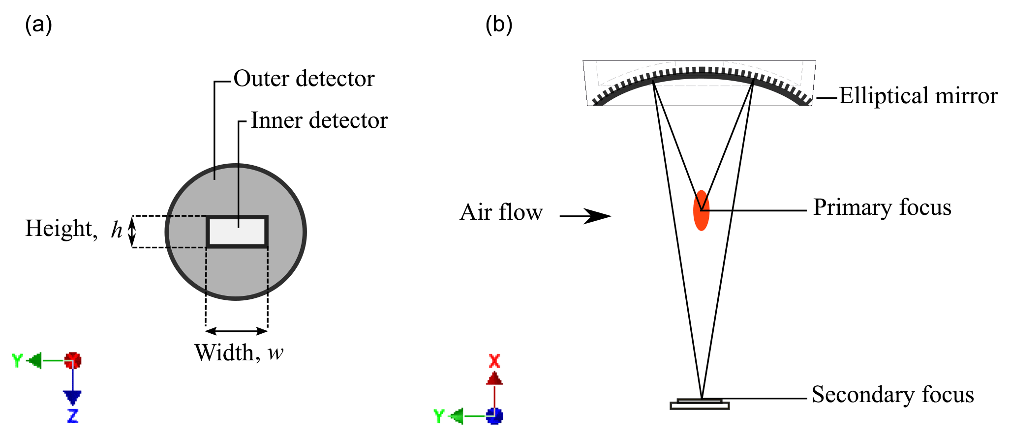
Figure 3(a) The dual-element detector consists of an inner rectangular detector of width, w, and height, h. (b) A view of the optical system orthogonal to the air flow: the laser beam is centred on the primary focus of the elliptical mirror, and the detector is centred at the secondary focus. The width, w, of the inner detector dictates the length of the laser beam (along the z axis, orthogonal to the air flow) in which a particle can be detected. The height, h, of the inner detector is wider than the path of a particle crossing the laser beam and therefore allows the entire pulse caused by a particle transit to be recorded.

Download

The geometry of the detector, mirror and laser are used to define the sensing area. As shown in Fig. 3ii, the focal point of the laser beam is located at the primary focus of the elliptical mirror and the detector is centred at the secondary focus. The inner detection area is a rectangle, where the width, w, directly governs the length of the laser beam (along the beam axis) in which a particle can be detected – and therefore defines one dimension of the sensing area. Figure 4 shows a rotated view of Fig. 3b, this time viewed in the direction of the air flow (the y axis). The image is also rotated slightly around the z axis in order to show the image formed on the detector. Figure 4a–c show how the width, w, of the inner detector governs the length of the sensing area in the z axis. In this direction, particles passing through the primary focus of the elliptical mirror will cause scattered light to be focused at the secondary focus. However, only those passing within $\pm \frac{\mathrm{1}}{\mathrm{2}}w$ of the centre of the sensing area will be focused onto the inner detector, whereas particles passing to the left or right will cause light to be focused onto the outer detector (as shown in Fig. 4c) and will not be counted. Figure 4d and e show how the focus of the elliptical mirror is used to define the dimension of the sensing area along the y axis. Particles passing above or below the primary focus of the mirror will cause scattered light to be focused above or below the detector – causing an enlarged image to form on the detector. In the current arrangement, particles passing 0.15 mm above or below the primary focus will create an image large enough to illuminate both the inner and outer detector, as shown in Fig. 4e, at which point the particle is considered to be outside of the sensing area. This distance is governed by the geometry of the mirror and the size of the inner detector. For particles straddling the boundary of the sensing volume, light will be focused onto both the inner and outer detectors, and therefore a criterion is defined to determine when the particle should or should not be counted. Based upon the intensity measured by the inner detector (I₁) and the intensity measured by the outer detector (I₂): if $I_{\mathrm{2}}\le \frac{\mathrm{1}}{\mathrm{4}}{I}_{\mathrm{1}}$ then the particle is considered to be inside the sensing area. The airflow is perpendicular to the sensing area, and, as such, all particles passing through the sensing area (occupying the x–z plane) will traverse the depth of the laser beam (in the y direction). The depth of the laser beam dictates the length of time the particle spends in the beam but does not dictate the number of particles sampled. We therefore define sample area and not sample volume. The total volume of sampled air is then calculated from the sensing area and the speed of the airflow.

Figure 4Optically defining the sensing area. The sensing area is shown as a shaded square within the laser beam, particles are represented by grey dots. The airflow direction is in the y direction. (a) Particles passing through the primary focus in the centre of the sensing area cause scattered light to be focused at the centre of the detector. (b) Particles passing to the left or right of the primary focus but still within the sensing area will cause scattered light to be focused to the right or left of the centre of the inner detector. (c) Particles passing more than $\frac{\mathrm{1}}{\mathrm{2}}w$ to the left or right of the centre of the sensing area will cause scattered light to be focused onto the outer detector. (d) Particles passing above or below the primary focus will cause the scattered light to be focused above or below the secondary focus and therefore above or below the detector, resulting in a larger image on the detector. (e) Particles passing more than 0.15 mm above or below the primary focus will cause scattered light to fall on both the inner and outer detector. The ratio of the inner and outer detector signals are used to determine whether particles are considered to be in the sensing area.

Download

Particles entering the sensing area will pass along the short axis of the focused laser beam (in the y direction) causing a pulse of light to fall on the detector. The width of this pulse is equal to the time of flight (ToF) of the particle across the beam, and the height of this pulse corresponds to the maximum intensity incident upon the detector during this transit. The pulse height depends upon the amount of light scattered by the particle, which is a function of particle size, optical properties and the intensity of the incident light. The pulse height is used to derive particle size, whilst ToF data are stored for data quality assurance. To ensure that the laser beam intensity is consistent across the sample area, the beam is clipped with the use of a 2 mm aperture, thus minimizing sizing errors due to beam non-uniformity. Figure 5 shows the relative intensity distributions across the major (left) and minor (right) axes. As discussed above, particles passing through the beam at the edges of the major axis will form unfocused images on the detector and therefore will not be counted; only the central 0.3 mm section of the major axis falls within the sensing area.

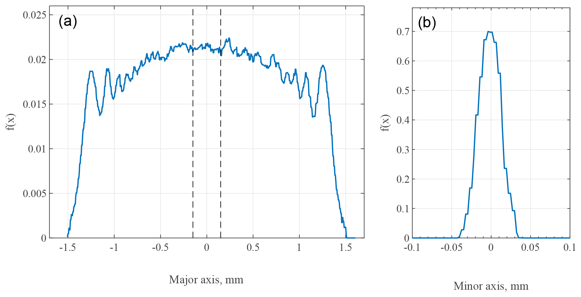
Figure 5Relative distributions of the laser intensity f(x) across the major (a) and minor (b) axes of the focused laser beam. Only particles passing within the central 0.3 mm of the major axis (shown as dashed lines) will be considered within the sensing area, and thus only these will be counted.

Download

2.3 Electronics

A PIC microcontroller-based (PIC18F27J53) electronic circuit governs the operation of the UCASS and how measurements using the dual-photodiode system are made and recorded. A simplified block diagram of the electronics system is shown in Fig. 6. As described above, the photodiode sensor consists of two photosensitive regions, the inner detector and the outer detector. A particle within the sensing area will cause some scattered light to fall incident on the inner detector, and this inner detector is used to create a trigger. The central element is connected to a circuit that converts the photo current to a voltage (0–3.3 V DC). The background signal is also monitored in order to account for stray light, as discussed in Sect. 2.2.1. The background signal is removed from the measured photocurrent, a process denoted here as “DC restoration”. The remaining signal will activate a trigger if the voltage amplitude detected goes above a predefined threshold (≈5 mV). In this event, the trigger comparator determines that there is a particle in the sensing area and notifies the core microcontroller. The microcontroller then activates the peak detector electronics that will sample and hold the peak of the light signal on both the inner and outer detectors as the particle passes through the laser beam. Before saving the peak value, a inner and outer signal ratio comparator is used to determine whether the particle is wholly within the sample area (as discussed in Sect. 2.2). If the particle is deemed to be within the sample area, then the microcontroller digitizes both signals with an on-board 12 bit analog-to-digital converter (ADC) and categorizes the combined peak signal into one of 4095 values (based on the resolution of the ADC) dependent upon the size of the amplitude. If the pulse height is too high, the detector will saturate and the particle will not be counted. This would be the case for the upper limit of the detectable size range. If the pulse is too low, the peak signal will not be sufficient to trigger a measurement and the pulse will not be recorded. This would be the case when the particle is below the threshold of the measurable size range.

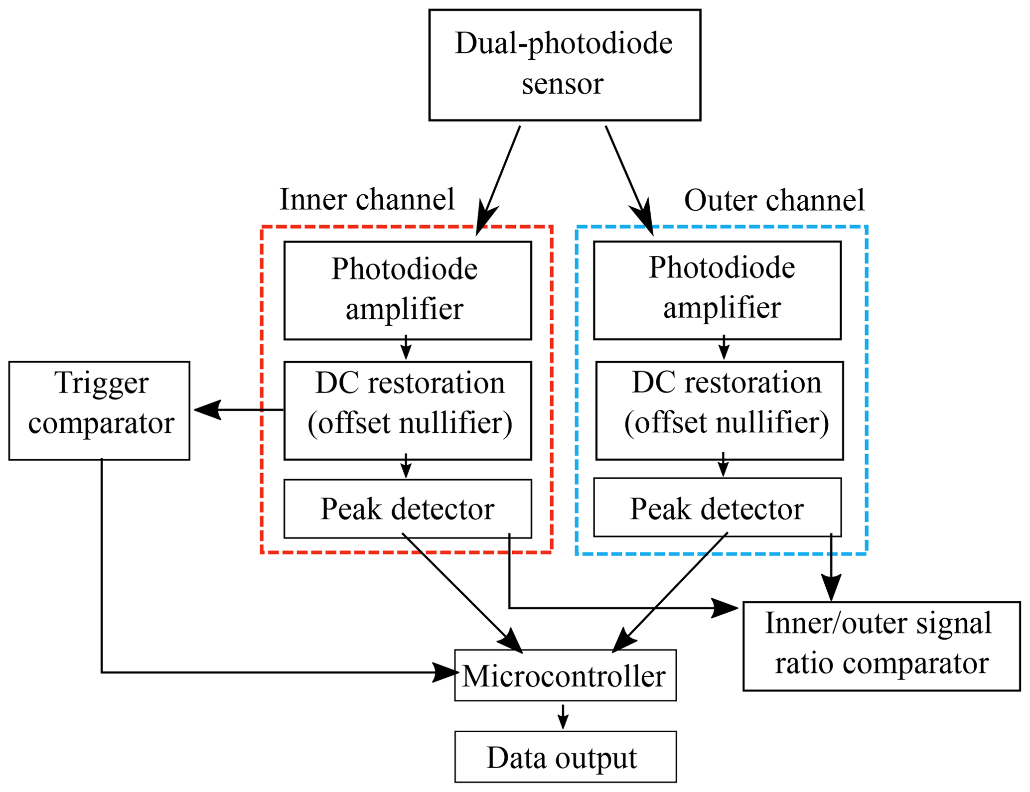
Figure 6Particles passing through the sensing area will cause light to fall on the inner element of the photodiode sensor. To account for stray light, the background signal is removed, a process labelled here as DC restoration. If the remaining signal on the inner channel goes above a threshold of 5 mV, the trigger comparator notifies the microcontroller that there is a particle within the sensing area. The signal's inner and outer channels are then measured to determine the total light incident on the detector (again, the background signal is removed). The inner and outer signal ratio comparator determines whether the particle is wholly inside the sensing area (as discussed in Sect. 2.2), and if the particle is deemed inside the sensing area, the data are saved.

Download

The measurable size range is determined by the laser power, amplifier gain and detector sensitivity. The amplifier gain can be adjusted by changing resistor values in the electronic circuit. Two versions of the UCASS hardware are available: a “high-gain” version with a nominal measurable size range of 0.4–17 µm and a “low-gain” version with a nominal measurable size range of 1–40 µm.

Particle-by-particle (PbP) pulse height recording is utilized during instrument calibration (discussed in Sect. 2.4.2); this utilizes all 4095 values of the ADC, allowing the digitized pulse for each particle to be recorded individually. However, during routine measurements, the data are aggregated into fewer size bins, with thresholds and limits defined by the user (up to a maximum of 16 bins). Measurements are rejected if the particle is deemed to be outside of the sample area (as discussed in Sect. 2.2), measurements are also rejected if the ToF is deemed too short or too long. A short ToF would occur if an event such as electrical noise spikes triggered the system. A long ToF would be the case if a large body or agglomeration of particles passed through the beam. The default ToF minimum and maximum limits are 1 and 100 µs, respectively. As the ToF is a function of particle size (amongst other factors), particles may produce legitimate ToFs above or below the rejection criteria. However, as the UCASS can only measure particles within a specific size range, the ToF rejection criteria are chosen such that particles within the measurable size range cannot realistically produce ToFs outside of the ToF criteria.

In this manner, the microcontroller continuously assembles histograms of particle size and count data. Means of ToF data are also recorded for a subset of the size bins to allow some use of this parameter to monitor flow rate through the device. At every 1 s interval, the histogram dataset is either saved to an on-board micro SD card or transmitted via a serial link (XDATA protocol) to a radiosonde device for radio frequency (RF) transmission of the data. The histogram data are cleared following each data save and transmit event. The XDATA protocol is limiting in terms of bandwidth, such that there is only space to utilize 10 of the available 16 size bins. The configuration of the bin boundaries can be altered to accommodate this and make best use of the bin quantity available. The device electronics can measure up to 10⁴ particles per second and can operate in air flow speeds between 2 and 15 m s⁻¹ with the standard firmware. For a standard operating velocity of 5 m s⁻¹, this equates to a particle concentration of 3.5×10⁹ m⁻³. The firmware can be modified to change the ToF window, thus allowing shorter or longer particle transitions to be recognized if the measurement platform requires it (this is discussed further in Sect. 3.1). Rather than coincidence, the most significant limit of the counting and sizing system is caused by the dead time of the microcontroller (MCU). This is the time the MCU takes to analyse a particle and increment a count in the appropriate size histogram bin. The system is insensitive to other particles entering the sampling volume during this time. The approximate dead time per particle is 40 µs processing time plus the particle transit time (≈10 µs). The 10⁴ counts per second rate limit stated is obtained by rounding the transit plus processing time approximation up to 100 µs and finding the reciprocal. In reality, aerosol is not perfectly homogeneous and particle detection events can be assumed to have a Poisson distribution. Where the counting frequency is significant compared to 10⁴ (e.g. >1000 s⁻¹), the proportion of coincidence events to valid events can start to become significant. However, in this research, the peak number concentration is recorded at $\approx \mathrm{2}\times {\mathrm{10}}^{\mathrm{7}}$, which equates to a counting frequency of ≈100 particles per second. At such counting frequencies the effect of dead-time coincidence is considered negligible.

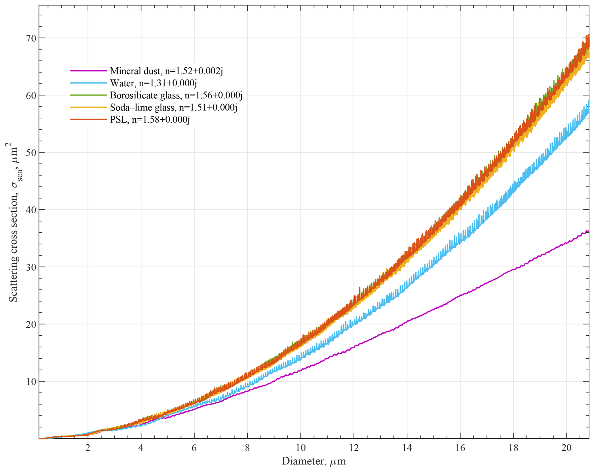
Figure 7Scattering cross sections, σ_sca, as a function of geometric diameter for mineral dust, water, borosilicate glass, soda–lime glass and polystyrene–latex (PSL).

Download

The size histogram bins utilized by the microcontroller are essentially levels of peak amplitude light signals scattered from measured particles. The bin boundaries are converted into particle diameters based on calibration using both theoretical and experimental data.

2.4 Calibration

2.4.2 Calibration measurements

To constrain the calibration curve, we take measurements of the instrument response for a series of National Institute of Standards and Technology (NIST)-traceable particle standards. These include PSL from Polysciences, borosilicate glass from Duke scientific and soda–lime glass from Whitehouse Scientific. A drying column is used to ensure the proper drying and dispersion of the calibration standards, whilst also establishing a stable, non-turbulent air flow through the UCASS. The experimental setup is shown in Fig. 8. The air intake consists of an initial drying chamber filled with silica gel desiccant, which dries the ambient air before passing it though a high-efficiency particulate air (HEPA) filter. This air is then directed through a series of tubes at the bottom of the drying column, which form a concentric ring around the aerosol input, thus establishing a clean, dry sheath flow into which the aerosol is injected. The purpose of the sheath flow is to accommodate the large volume of air flowing through the instrument. By having a clean, dry sheath flow, calibration particles only need to be contained within the centre of the airflow, allowing them to travel through the sensing area, therefore fewer particles are wasted in the process. The main drying column consists of a 1 m tall tube with an inner tube for the airflow. The outer tube is packed with silica gel desiccant and the inner tube is lined with a microporous membrane. This combination aids the drying of any aerosol injected into the sheath flow, which will be fully dried before reaching the UCASS at the top of the column. A vacuum pump is used in line with the UCASS to establish an air flow of 3–5 m s⁻¹ (the intended operational velocity of the UCASS). Two different aerosol input techniques are used for wet and dry dispersion. The PSL microspheres are suspended in an aqueous solution and are aerosolized using a TSI Tri-Jet 3460, which is fed directly into the sheath flow. To disperse the dry calibration standards, a small amount of beads are placed into a small dispersion bottle consisting of an inlet and outlet tube. A burst of dried, filtered air in the inlet pipe creates a turbulent environment inside the bottle which aids the breakup of any agglomerates. The outlet pipe is then directed into the sheath flow and the dispersed particles are carried in the airflow through the UCASS.

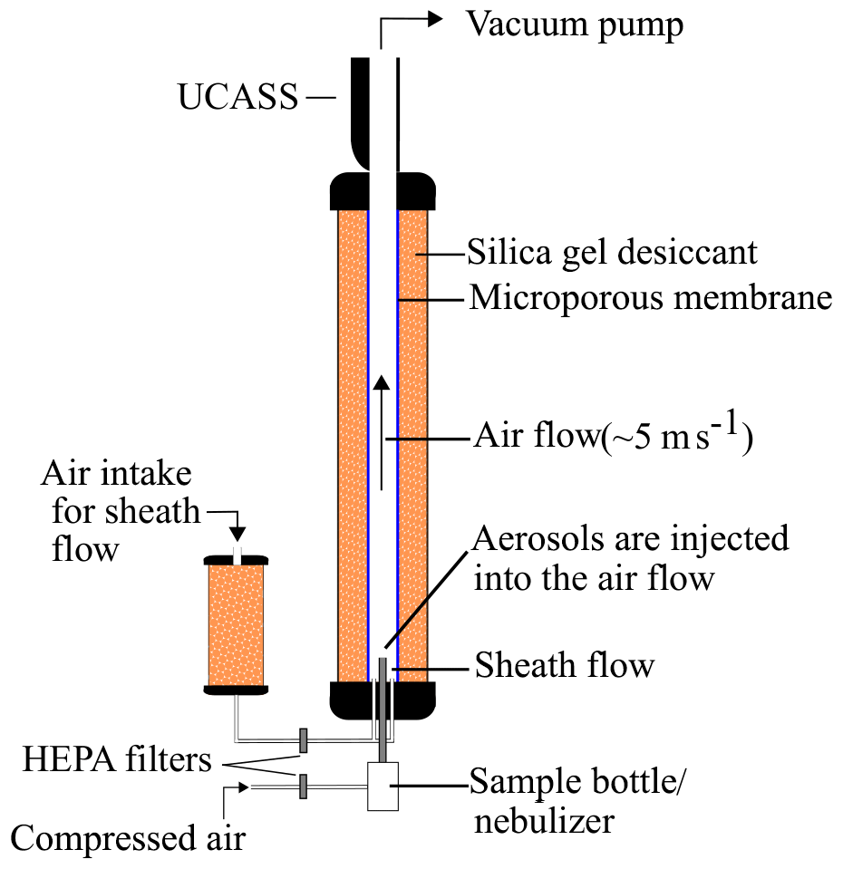
Figure 8Experimental setup used to take calibration measurements. A vacuum pump is used to draw air through the drying column. The air intake is taken from ambient air that is first passed through desiccant and then a HEPA filter. This clean dry air is then directed through a concentric ring of pipes at the bottom of the drying column to create a clean, dry sheath flow. The aerosol is then injected into the sheath flow via the TSI tri-jet aerosol generator (for wet dispersion) or via a sample bottle for dry particles. The sheath flow constrains the aerosol in the centre of the air flow, which is carried directly through the sensing area of the UCASS.

Download

As discussed above, to avoid sizing uncertainties associated with bin width during calibration, a calibration-specific firmware is utilized, which allows particle-by-particle (PbP) pulse heights to be recorded. Measurements of various calibration standards are shown in Fig. 9. Figure 9a shows measurements from the high-gain version of the UCASS, which has a nominal sizing range of 0.4–17 µm, and Fig. 9b shows measurements from the “low-gain” version of the UCASS, which has a nominal sizing range of 1–40 µm. Calibrations are always conducted with the maximum number of particle standards available, and the data presented in Fig. 9 show all available standards at the time of publishing. The UCASS units used for the experiments presented in Sect. 3 were calibrated using five (or more) point calibrations using the particle standards available at the time. Although PSL and glass beads are typically considered monodisperse for calibration purposes, the full size range can be broad. Therefore, the full size distribution of the aerosol is measured, and the mean, median and modal value of the whole distribution are found. Manufacturers may describe the average size of their test particles using different averages, and therefore it is necessary to select the correct average for each sample type. For these calibrations, the mean values are used for PSL and soda–lime glass, whereas the median is used for borosilicate glass. In cases where the full distribution is not captured, the modal value is used. This occurs in the case that the full size range of a particular sample may extend beyond the measurable limits of the instrument. For example, in Fig. 9, the largest diameter aerosol used in this calibration is 14.4 µm, and it can be seen that the distribution is cut off at the point where the detector saturates. The same occurs for the low-gain version for the 37.36 µm sample. In these cases, the full distribution could not be measured, and therefore the mean or median cannot be used, thus the modal value is used instead.

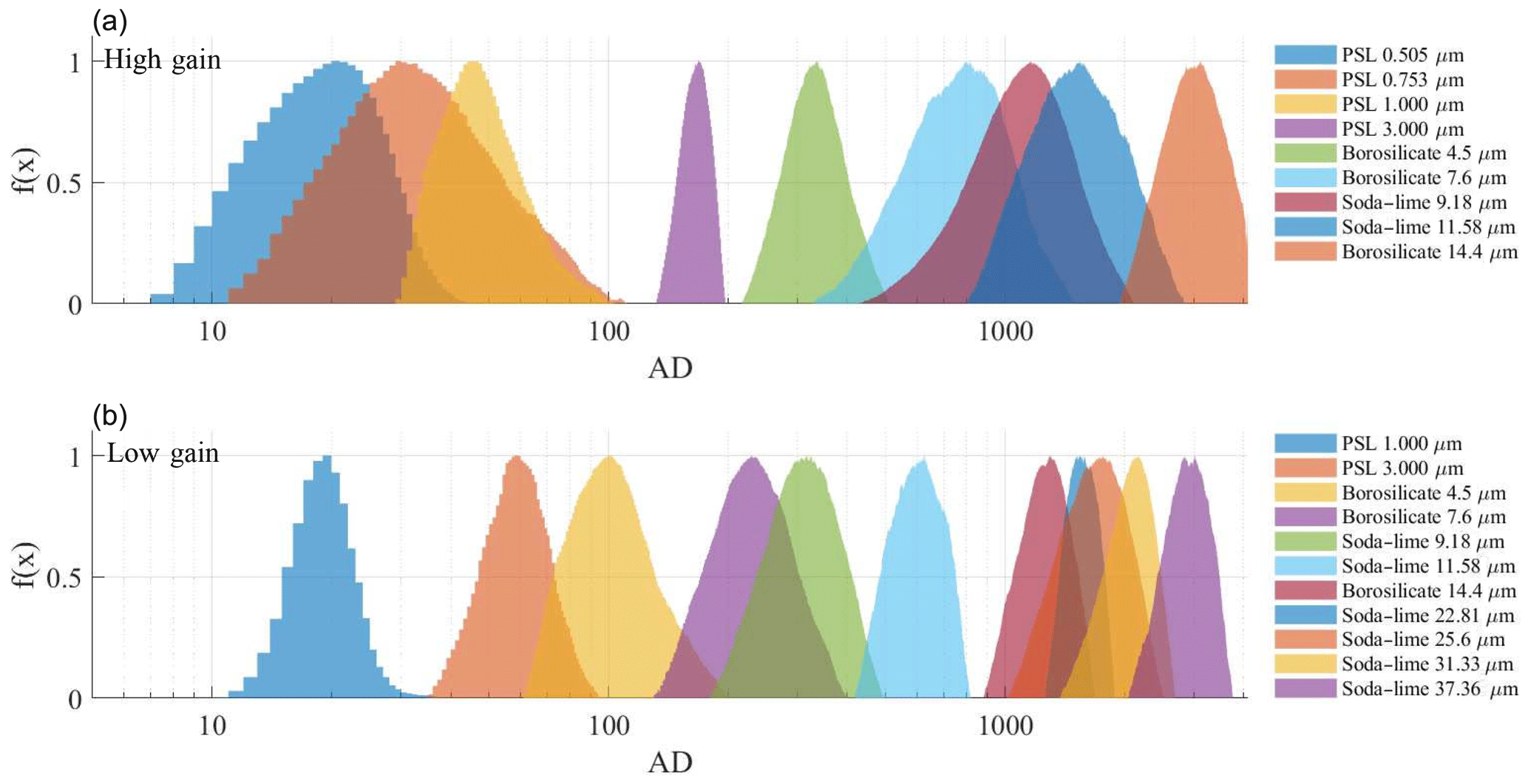
Figure 9Measured instrument responses for various NIST-traceable calibration standards, including PSL, borosilicate glass and soda–lime glass. f(x) is the normalized counts, as measured by the instrument; for presentation purposes, each distribution is normalized to a peak height of 1. Panel (a) shows measurements conducted using a “high-gain” version of the UCASS, and panel (b) shows measurements conducted using a “low-gain” version.

Download

Theoretically, the instrument response is directly proportional to the scattering cross section. However, the instrument response may differ from the theoretical response due to manufacturer tolerances in the optical and electronic components. Some variations, such as laser power and amplifier gain, will cause constant offsets over the measurement range. However, some offsets may be non-linear due to the varying signal-to-noise ratio (SNR) across the measurement range and non-linearity in the detector sensitivity. To account for all offsets, the log of instrument response (analog-to-digital counts, AD) is plotted against the log of the scattering cross section and a line of best fit is applied, as shown in Fig. 10.

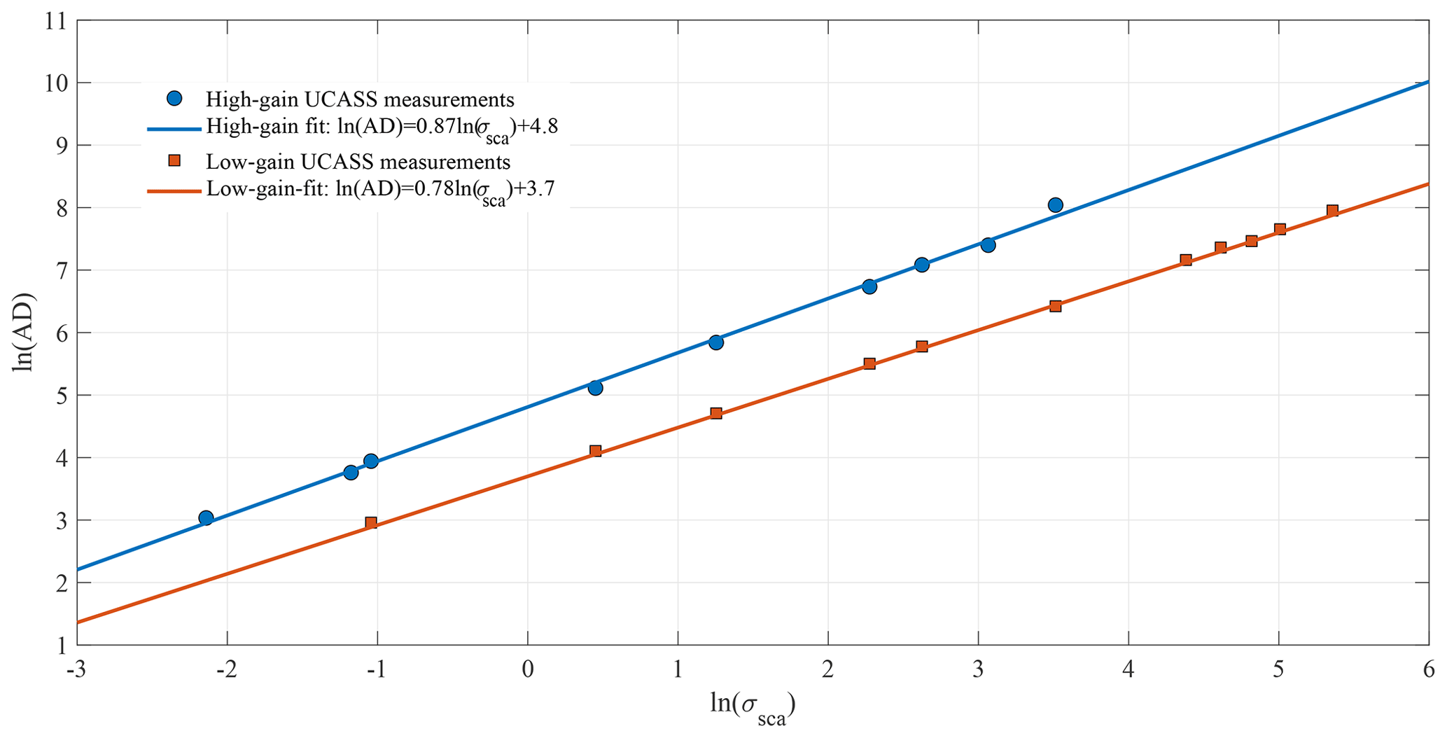
Figure 10The log of the measured instrument response (AD) is plotted against the log of the scattering cross section (σ_sca) for the calibration standards used. For PSL and Duke Scientific borosilicate glass beads, the mean instrument response is used, as this is how the manufacturer specifies the particle size. For the Whitehouse Scientific soda–lime glass beads, the sample size is defined by the median, and thus the median instrument response is plotted.

Download

A linear fit is applied to link the scattering cross section to the instrument response. For the examples shown, the relationship for the high-gain UCASS is given by

$$\begin{array}{}\text{(4)}& \ln \left(\mathrm{AD}\right)=\mathrm{0.87}\ln \left({\mathit{\sigma }}_{\mathrm{sca}}\right)+\mathrm{4.8},\end{array}$$

and the relationship for the low-gain UCASS is given by

$$\begin{array}{}\text{(5)}& \ln \left(\mathrm{AD}\right)=\mathrm{0.78}\ln \left({\mathit{\sigma }}_{\mathrm{sca}}\right)+\mathrm{3.7}.\end{array}$$

These equations can then be applied to any particulate (e.g. mineral dust, water) by computing the scattering cross sections for discretized diameters across the measurement range and relating the instrument response to the particle diameter. Using this technique, finalized calibration curves are produced for five materials: PSL, soda–lime glass, borosilicate glass, water and mineral dust, as shown in Fig. 11. If a priori information of the aerosol type is known, then the calibration curve can be chosen to best suit the application. The calibration curve can then be used to select the boundaries of up to 16 size bins (this is limited to 10 if interfacing the UCASS via XDATA protocol). Since the relationship between ln (AD) and ln (σ_sca) remains valid for any material and shape of aerosol. If post factum information on the particle shape or refractive index becomes available (i.e. via analysis of co-located measurements), then a post calibration can be applied.

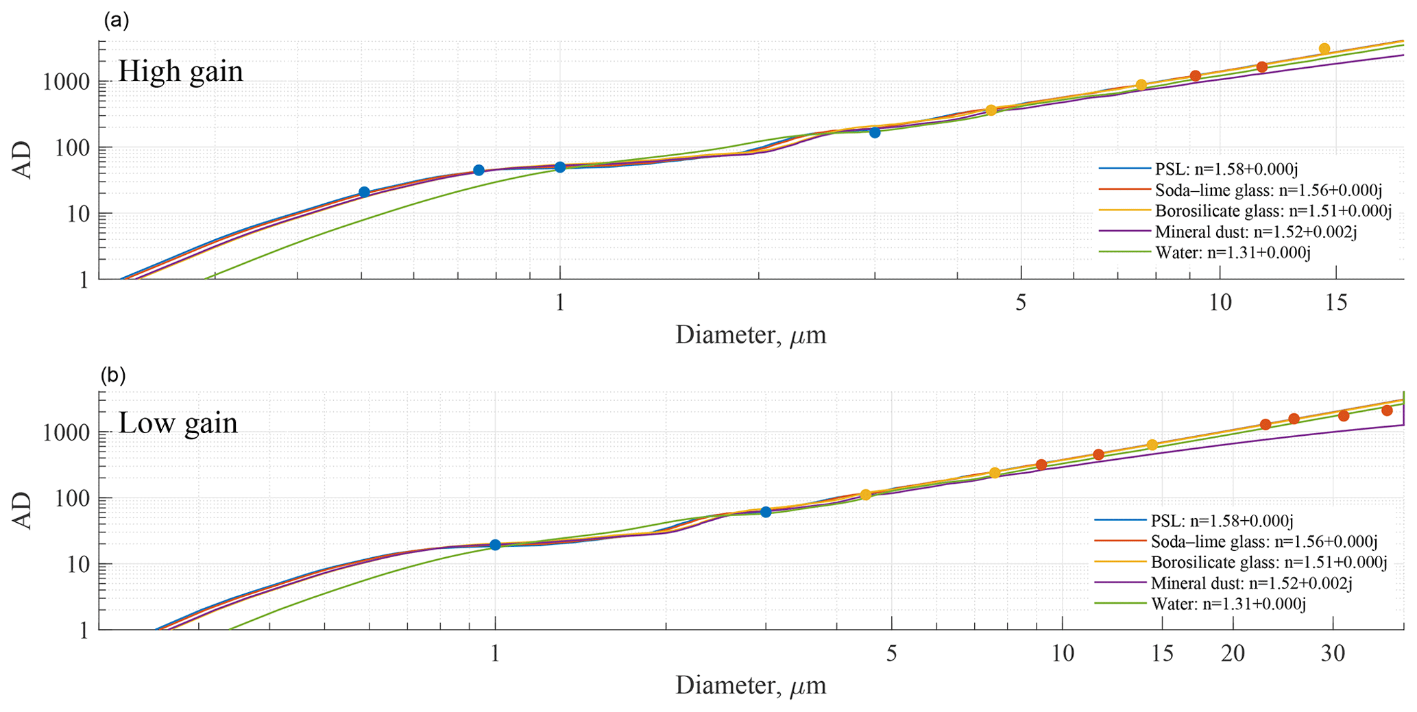
Figure 11Final calibration curves for a high-gain (a) and low-gain (b) UCASS. The geometric diameter is plotted against instrument response for varying materials. The measured values (as shown in Fig. 9) are overlaid on the calibration curves and shown as filled circles, where the colour denotes the material. If a priori information of the refractive index is known, the calibration curve can be selected to best suit the material being measured. If post factum information about the material becomes available, the calibration can be adjusted.

Download

2.5 Evaluation of air flow uncertainty

The UCASS is a naturally aspirated system, by which an external air flow (relative to the UCASS) is required to transport particles through the sensing area. The main advantage of this setup is the reduction of particle loss mechanisms induced by complex aerodynamic systems and non-isokinetic sampling, which has been evaluated empirically for artificially aspirated systems (Spiegel et al., 2012; Hangal and Willeke, 1990; Von Der Weiden et al., 2009). However, the sampling efficiency is still dependent on the axial characteristics of the external airflow, hence a range of accepted (aerodynamic) operating conditions must be defined. To understand the airflow through the sample area, computational fluid dynamics (CFD) using the “Star CCM+” commercial code are used to model the air flow through the instrument at varying angles of attack. The CFD simulation is a two-dimensional model on the symmetry plane of the UCASS, this was chosen because the velocity of an “air parcel” in a subsequent plane to this is likely to be similar, meaning the viscous stress between planes is negligible. The fundamental equations behind this CFD are the Reynolds-averaged Navier–Stokes (RANS) equations, which were chosen for computational efficiency when compared to direct numerical simulation.

Figure 12 shows the air flow through the UCASS for an external velocity of 5 m s⁻¹. For an axial air flow, the air velocity through the sample area is 5.6 m s⁻¹, 12 % higher than the external air flow. Whilst the drag on the inside walls of the UCASS causes the airflow to slow down, the sample area lies outside this boundary layer and is therefore subject to a slightly higher air speed. The UCASS inlet is asymmetric due to the design constraints making it compatible with the KITsonde dropsonde system, and therefore we must also consider the effect of tilt in different directions. As the UCASS is tilted upwards, the air flow through the sample area increases; however, as it is tilted downwards, the air speed decreases. This relationship between tilt and air speed is asymmetric, with negative angles of attack having a greater impact on the air flow. Therefore, to retrieve reliable concentration measurements from the UCASS, the airflow or angle of attack must be known.

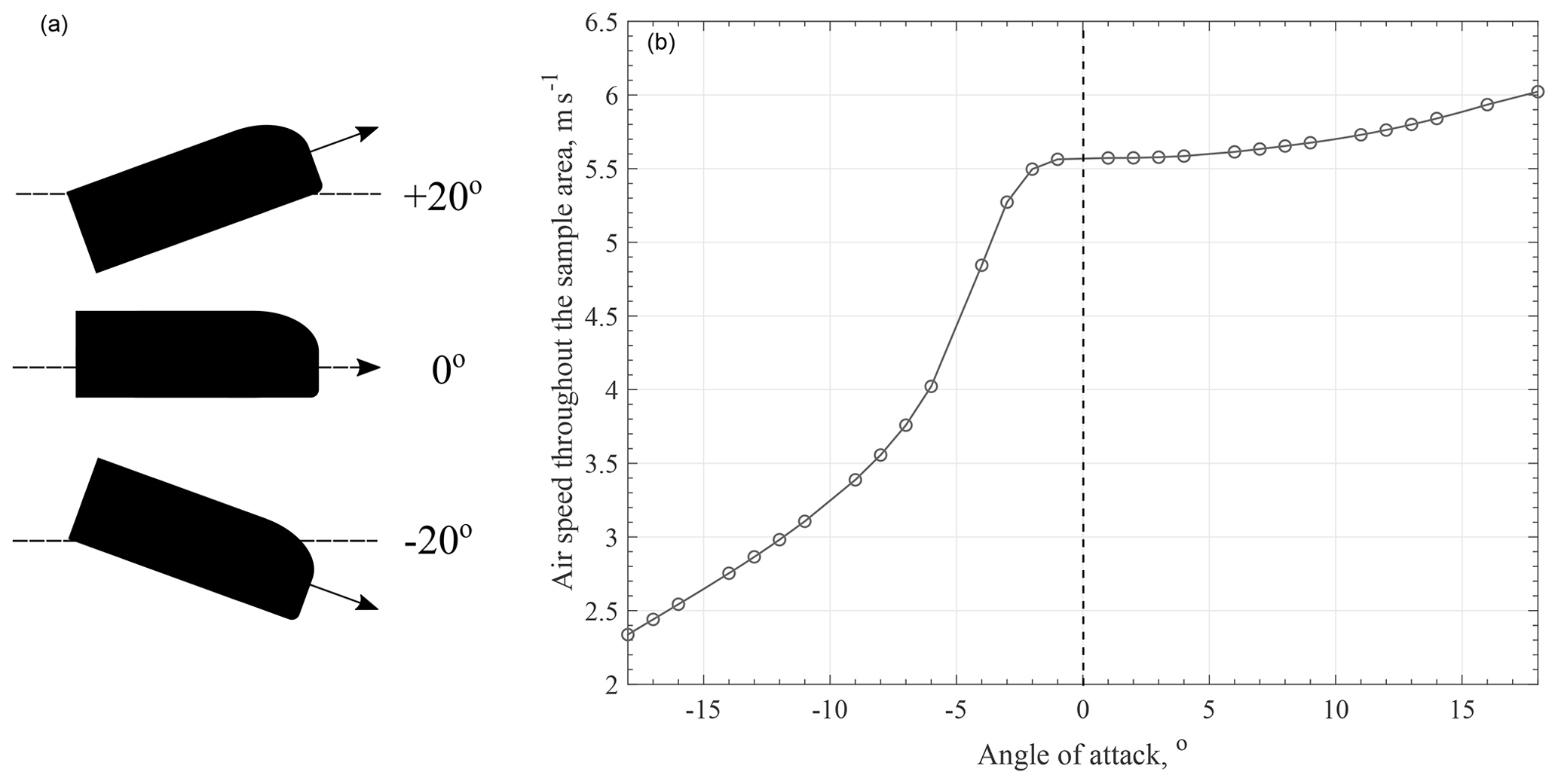
Figure 12Model results showing the air velocity in the sensing area. Panel (a) shows how the tilt direction is described in relation to the instrument geometry. Panel (b) shows the simulated flow velocity in the sample for tilt angles between −20 and 20^∘ in an external air flow of 5 m s⁻¹.

Download

When the UCASS is launched on a meteorological balloon, the balloon–payload configuration acts as a pendulum system. To constrict the movement of the UCASS, the payload is configured as a double pendulum, whereby the UCASS is secured by a line below the balloon and the meteorological sonde is secured below the UCASS. This double pendulum configuration allows fast energy dissipation while at the same time ensuring small amplitude of the UCASS oscillations, generally smaller than the amplitude of the lowest element, the radiosonde. Although the UCASS still oscillates, model results show that the tilt is constrained to within ±5^∘ as shown in Fig. 13.

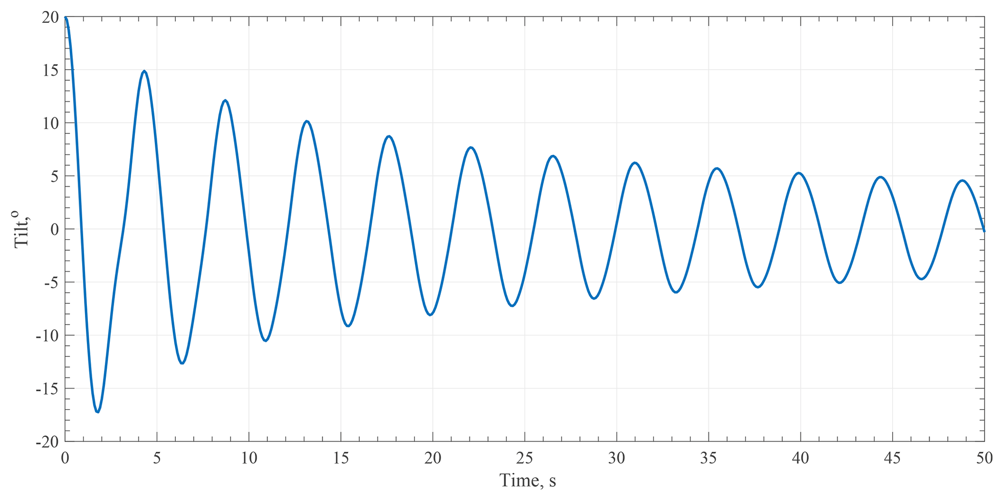
Figure 13Model results showing the angular tilt of the UCASS with respect to the direction of ascent. Initial oscillations can reach ±20^∘, although these are damped after ≈30 s and constrained within ±5^∘.

Download

By constraining the tilt of the UCASS within these limits, model results show that the mean air speed through the sample area is equal to 5.4 m s⁻¹, with a standard deviation of 0.3 m s⁻¹, which is used to compute the number concentrations. For dropsonde systems, a similar configuration is used, whereby the sonde is tethered between the parachute and the meteorological sonde and the angle of tilt is constrained to within the same boundaries.

3.1 Laboratory inter-comparisons

Inter-comparison tests were conducted in laboratory settings to assess the sizing and counting ability of the UCASS in comparison to reference instrumentation.

3.1.1 Sizing comparisons

To assess the sizing ability of the UCASS, a TSI 3300 optical particle sizer (OPS) is used to measure the same particle calibration standards as discussed in Sect. 2.4.2. The TSI OPS is an optical particle counter, capable of sizing and counting particles in the 0.3–10 µm range in 16 user-configurable size bins. For comparative purposes, the TSI was set to the finest size resolution for each measurement, focusing only on the size range of interest. The results are compared to the measurements taken by the UCASS while in particle-by-particle mode (as discussed in Sect. 2.4.2). Measurements are also compared with statistical values given by the manufacturer of the particle standard, where available. These measurements are shown in Fig. 14.

Figure 14Measurements of particle size distribution from the TSI 3330 OPS, the high-gain UCASS and the low-gain UCASS. Manufacturer values are also shown, where available. Data for PSL and borosilicate standards are summarized in Table 1, while data for soda–lime samples are summarized in Table 2.

Download

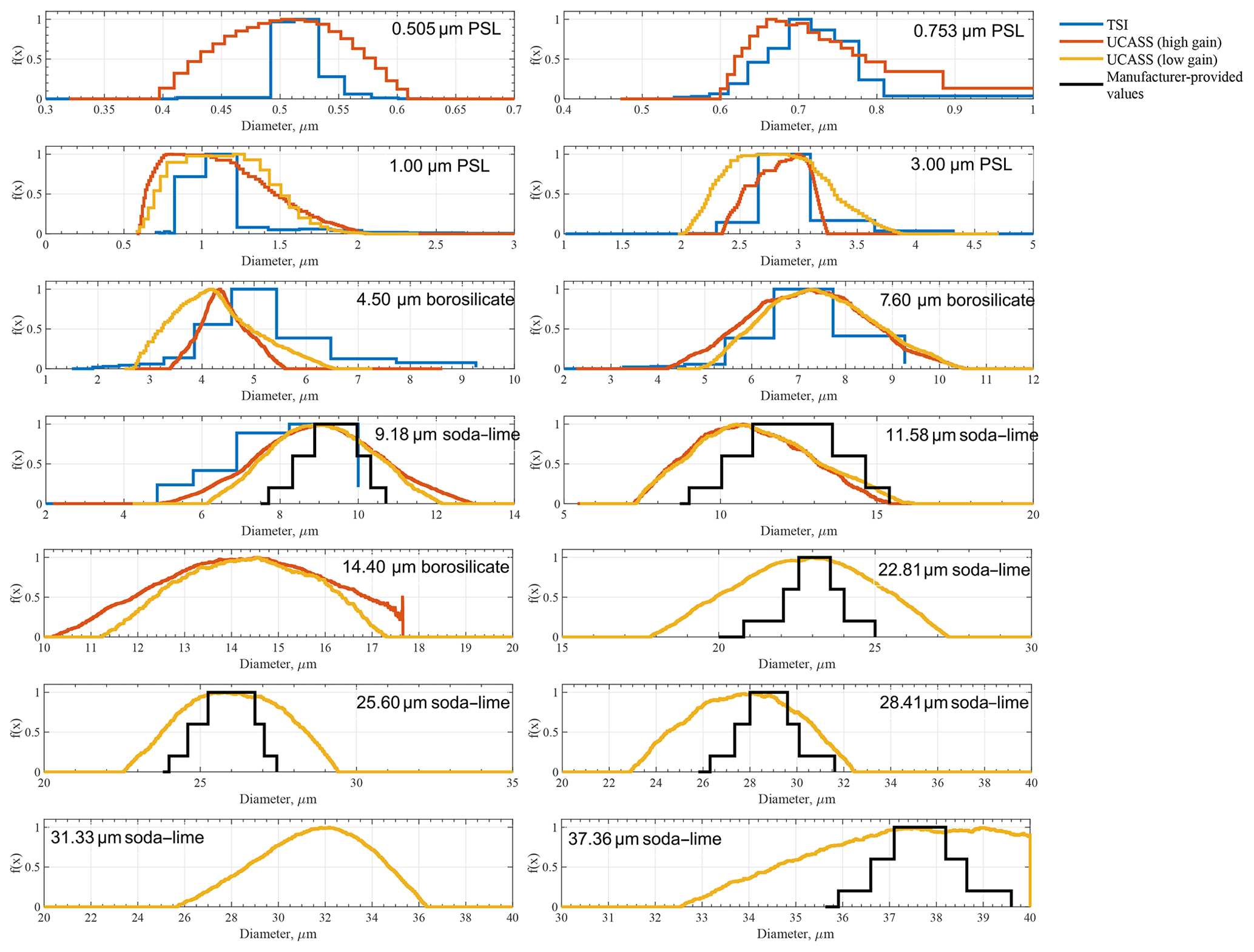
Table 1Numerical summary of data shown in Fig. 14 pertaining to PSL and borosilicate particle standards. The first column shows the mean and standard deviation of calibration standards as given by the manufacturer. The remaining columns show distributions measured by the TSI OPC, the high-gain UCASS and low-gain UCASS. Incomplete distributions (i.e. where the full size distribution exceeds beyond the measurable size range) are denoted with an asterisk.

Download Print Version | Download XLSX

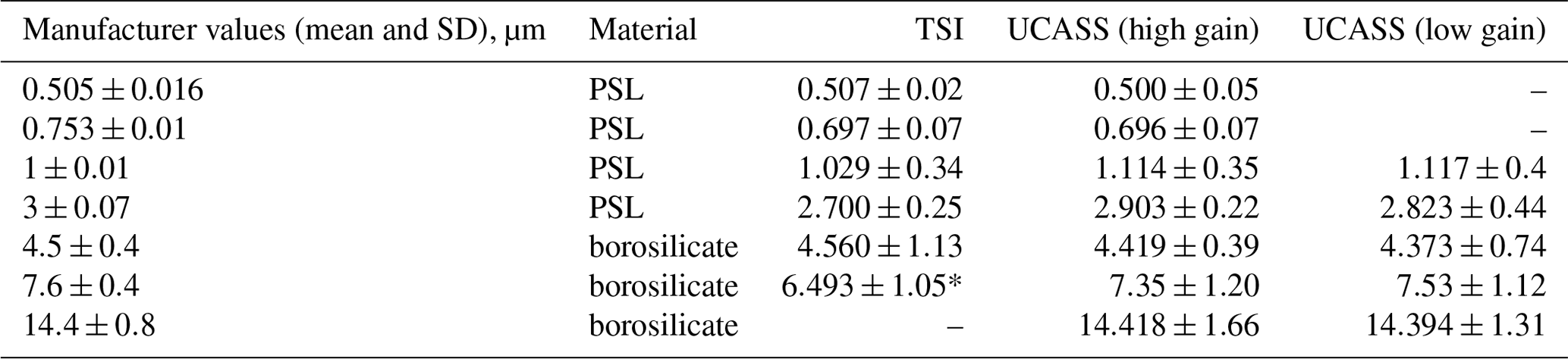
Table 2Numerical summary of data shown in Fig. 14 pertaining to soda–lime glass particle standards. The first column shows the median and interquartile range (iqr) of calibration standards as given by the manufacturer. The remaining columns show distributions measured by the TSI OPC, the high-gain UCASS and low-gain UCASS. Incomplete distributions (i.e. where the full size distribution exceeds beyond the measurable size range) are denoted with an asterisk.

Download Print Version | Download XLSX

3.1.2 Counting comparisons

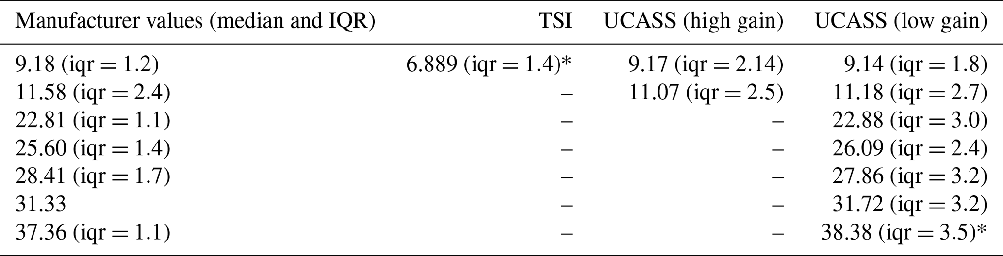
To assess the counting ability of the UCASS, an aerosol chamber was filled with polydisperse aerosol. The polydisperse aerosol was generated using a vaporizer containing a mixture of propylene-glycol and vegetable glycerine. The TSI was mounted in the chamber and sampled continuously, the UCASS was mounted nearby the TSI and a pump attachment was used to draw air through the inlet. Measurements were repeated using different size bins in order to collect data across the full measurable range (0.4–10 µm) and with a higher resolution at smaller sizes. Typical concentrations during the experiment were of the order of 10³ cm⁻². The measured concentrations of the UCASS are compared to the measured concentrations of the TSI in Fig. 15, where the data are averaged over all experiments and the error bars represent standard deviations. A dotted line represents the 1:1 ratio (i.e. UCASS concentration is equal to TSI concentration). It can be seen that the ratio of measured concentrations varies between 0.8 and 1.2 across all size ranges, and therefore the two instruments agree to within 20 %. For 19 out of 20 measured size ranges, the 1:1 ratio lies within the standard deviation of the data.

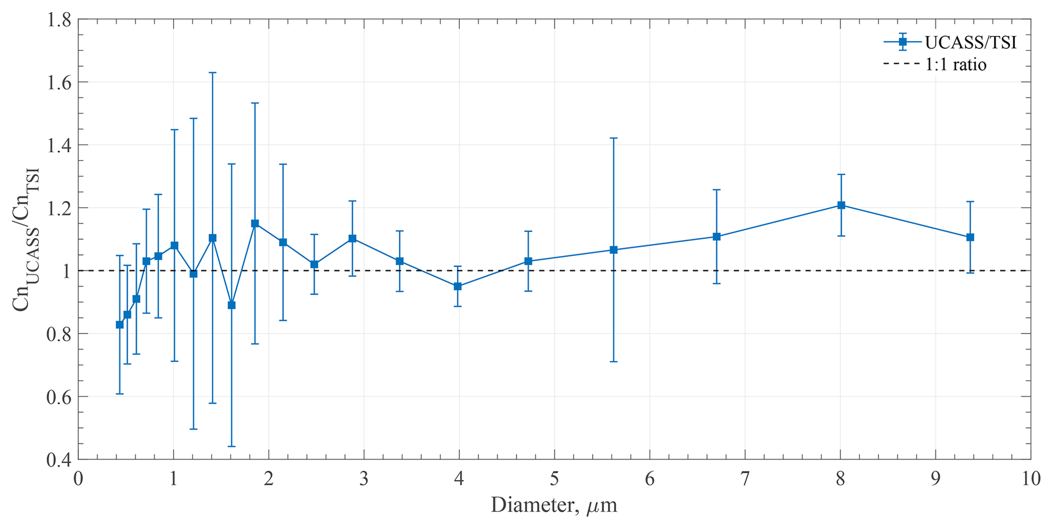
Figure 15Ratio of UCASS-measured number concentrations (Cn^UCASS) to TSI-measured number concentrations (Cn^TSI), where data points represent means averaged over 100 readings and error bars represent standard deviations. The 1:1 ratio is shown as a dashed black line.

Download

3.2 In situ intercomparisons

A low-gain configuration of the UCASS (calibrated for water droplets) was tested at the Observatoire de Physique du Globe de Clermont-Ferrand (OPGC) observatory, located atop the Puy De Dôme volcano at an altitude of 1465 m. The observatory consists of a rooftop measurement platform with an integrated wind tunnel capable of pumping through the passing clouds. As the UCASS requires an external air flow, the UCASS was tested in the wind tunnel, co-located with a cloud droplet probe (CDP-2) from Droplet Measurement Technologies (DMT) (Lance et al., 2010). The CDP-2 is an open-geometry system that provides size and concentration measurements in the range 2–50 µm and is intended for air speeds of 10–250 m s⁻¹. During a stratocumulus event, the UCASS and CDP were co-located in the wind tunnel and the cloud was drawn through at varying speeds from 5 m s⁻¹ (the lowest operational velocity of the wind tunnel) to 20 m s⁻¹. Figure 16 shows the measured liquid water content (LWC) taken by the UCASS (blue) and the CDP (orange). Both instruments measured at a rate of 1 Hz (shown by dotted lines), and the solid lines represent the smoothed data, using a 10-point moving average. The air speed is shown via a dotted green line corresponding to the right-hand y axis. It can be seen that throughout the experiment both the UCASS and CDP capture the same temporal variations in the liquid water content, although the magnitudes start to diverge at air velocities above 17 m s⁻¹. This under-counting by the UCASS is expected due to the short ToF (discussed in Sect. 2.3), which causes the particles to be rejected. This ToF threshold is intended to prevent miscounting of short pulses, which can be caused by electrical noise. However, the ToF limits can be altered to suit the measurement platform. In the overlapping measurement range (air speeds between 10 and 15 m s⁻¹), the ratio of UCASS-measured LWC to CDP-measured LWC is equal to 1.02.

Figure 16(a) Measured liquid water content (LWC) by co-located UCASS and CDP instruments at varying air speeds. The two instruments were installed side-by-side in the wind tunnel at Puy de Dôme during a stratocumulus event, and the air speed was increased from 5 to 20 m s⁻¹. (b) Ratio of the LWC measured by the UCASS to the LWC measured by the CDP. The dotted black line shows the 1:1 ratio.

Download

3.2.1 Dropsonde system

Dropsondes were launched from the Dornier 128 aircraft north of Magdeburg, Germany, on 3 August 2013. The packages contained the UCASS in tandem with KITsondes (Wieser et al., 2014), for co-located particle and meteorological data. The size distribution profiles measured by the UCASS indicated mineral dust present in the free troposphere during 3 August for a drop conducted at 13:10 UTC. At 15:34 UTC, AERONET sun photometry retrievals (Dubovik and King, 2000) from IfT Leipzig (located 100 km south-south-east of Magdeburg) confirmed the presence of dust. The integrated size distribution measured by the UCASS is compared to the AERONET inversion from Leipzig in Fig. 17a. The size distribution is integrated for the column between 3 and 5 km to exclude boundary layer aerosol over the Colbitz-Letzlinger Heide area (the EDR74 exclusion zone). Figure 17b shows the dust dispersion model for 12:00 UTC using the MACC (Monitoring Atmospheric Composition and Climate) forecast, showing the transport of dust over Germany from the Sahara. The locations of Magdeburg and Leipzig are marked by red and yellow crosses, respectively.

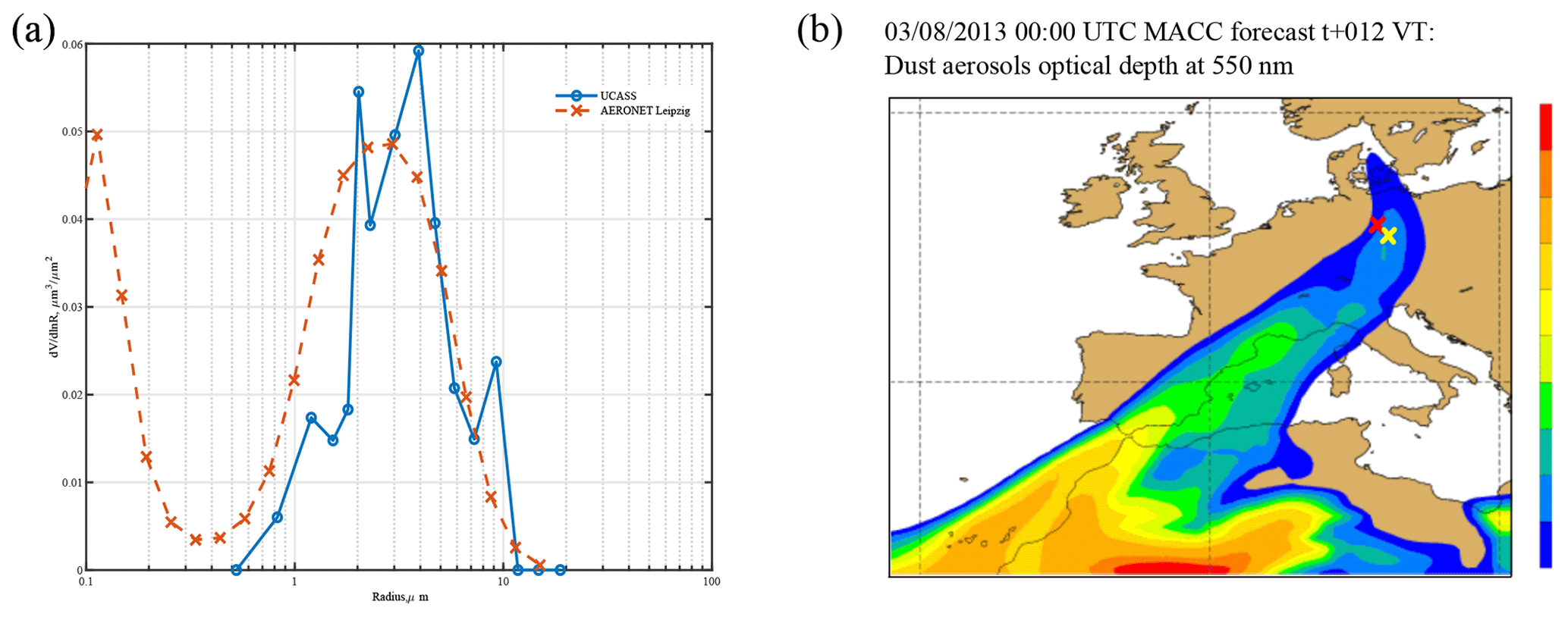
Figure 17(a) Integrated aerosol size distribution measured by the UCASS compared with the AERONET inversion (as retrieved from the sun photometer data) from Leipzig. (b) Dust dispersion model showing Saharan dust transport over Leipzig (marked by a yellow cross) and Magdeburg (marked by a red cross).

In a further drop during this dust event, a UCASS dropsonde system was deployed 3 min later at 13:13 UTC. This payload measured a thin, embedded cloud layer as shown by high number concentrations at larger sizes at 4 km. This is illustrated in Fig. 18a, where the number concentrations for each of the 16 size bins are shown. Over the 6 km profile, the majority of particulates counted measured less than 3 µm in diameter, except for a thin layer at 4 km with high concentrations of particles in larger size bins. This change in concentration and size suggested the presence of a thin cloud layer, which was confirmed by the humidity profile measured by the attached KITsonde shown in Fig. 18b, which measured high humidities at 4 km. Figure 18c shows the effective diameter with respect to altitude, it can be seen that the Saharan dust layers above or below the cloud have an effective diameter of ≈2 µm. At 4 km when the UCASS enters the cloud layer, this effective diameter steeply increases to ≈6 µm. As discussed in Sect. 1, dust can cause the formation of clouds by acting as a cloud condensation nuclei, thus embedded clouds during dust events are not uncommon. However, the presence of cloud presents difficulties for remote sensing instrumentation, and therefore retrievals are not possible for cloud-contaminated datasets. So long as the UCASS is launched in tandem with a meteorological sonde, the measured humidity profiles can be used to differentiate between cloudy and non-cloudy conditions, and therefore the UCASS can be used to measure both cloud and aerosol size distributions even when both are present.

Figure 18(a) Number concentration of particulates in the 16 UCASS size bins with respect to altitude, suggesting an embedded cloud layer at 4 km. (b) Temperature and relative humidity profiles from the attached KITsonde, also suggesting an embedded cloud layer at 4 km with a spike in humidity. (c) Effective diameter with respect to altitude, the embedded cloud layer at 4 km is evident due to the steep increase in effective diameter. The blue line shows raw data, whilst the orange line shows smoothed data using a 10-point moving average.

Download

3.2.2 Upsonde system

The UCASS was used during the AERosol properties – Dust (AER-D) and Sunphotometer Airborne Validation EXperiment – Dust (SAVEX-D) campaigns over Cabo Verde during August 2015 (Marenco et al., 2018). A UCASS was launched as part of a balloon-based system in tandem with a GRAW DFM-09 during a Saharan dust event on 25 August, from Instituto Nacional De Meteorologia e Geofisica (INMG), Espargos, Sal island. The launch was conducted at 17:01 UTC from ground level (70 m above sea level), this launch was timed to coincide with a deep profile (profile 6) conducted by SAVEX-D flight no. B934. The research aircraft started the profile from an altitude of 4 km at 17:10 UTC off the west coast of Boa Vista island (≈0.75 ^∘ S, 0.15 ^∘ W of the balloon launch site). The aircraft then flew due north, passing Sal island until reaching an altitude of 690 m. Figure 19a shows the flight paths of the aircraft and balloon (up to 4 km), whilst Fig. 19b shows the altitude of both profiles with respect to time. Figure 19c shows the near-real-time dust forecast from the Met Office Global Atmosphere model (Martin et al., 2018) for 18:00 UTC, where it can be seen that dust is advected westwards from the Sahara. The circular section shows a zoomed-in image over the Cabo Verde islands, and the islands of Sal and Boa Vista are highlighted by a red rectangle. It can be seen from the forecast that the aircraft and balloon profiles were conducted at the leading edge of a dust layer, and therefore, even though the spatial and temporal differences between the two profiles are minimal, some variability in the dust layer may be expected.

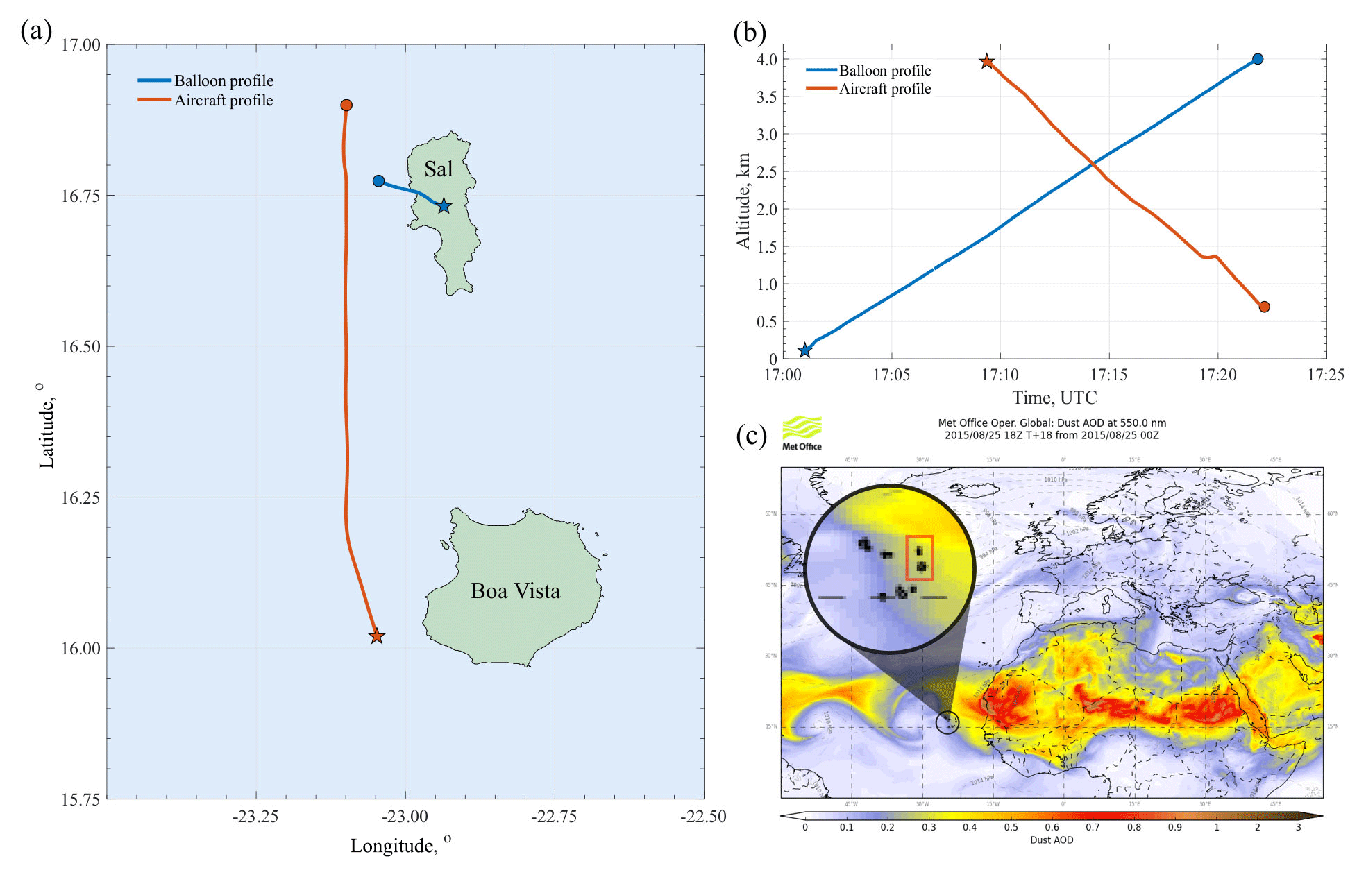
Figure 19A balloon launch was conducted to coincide with profile 6 of SAVEX-D flight B934. Panel (a) shows the flights paths of the balloon (blue) and aircraft (orange) during this profile, where the start and end points are marked by stars and circles, respectively. The altitudes are shown in (b), whereby the aircraft descends from an altitude of 4 km to 690 m. For comparative purposes, only the balloon data up to an altitude of 4 km are shown here. Panel (c) shows the MET office global atmosphere model aerosol optical depths (AODs) for 18:00 UTC. The Cabo Verde islands are zoomed-in and the islands of Sal and Boa Vista are highlighted in a red rectangle. It can be seen from this that the measurements were located to the edge of a dust layer, with an anticipated AOD of ≈0.3.

Figure 20a shows the mass concentration profile measured by the UCASS, compared with measurements from the aircraft-mounted PCASP (Passive Cavity Aerosol Spectrometer Probe). The PCASP is an aircraft-mounted OPC by Droplet Measurement Technologies. Similarly to the UCASS, the PCASP utilizes wide-angle scattered light, with the primary reflector covering the angular range 35–120^∘. For comparative purposes, the mass concentrations shown only apply to the overlapping measurable size range of the UCASS and PCASP, in this case the size range is from 0.4 to 3 µm, corresponding to the first seven bins of the UCASS. Figure 20b shows the ratio of the mass concentrations measured by the UCASS and PCASP, respectively. Over the 4 km profile, the average ratio is 1.2, with the greatest differences between the two measurements occurring at the base and top of the dust layer (≈1.6 and 4 km, respectively). The dust layer was advected from the east, as shown in Fig. 19, thus the spatial separation between the two profiles explains the discrepancies. The more easterly UCASS measurement captures higher concentrations and a higher layer height, whilst the more westerly PCASP measurement measures a lower layer height, likely due to gravitational settling.

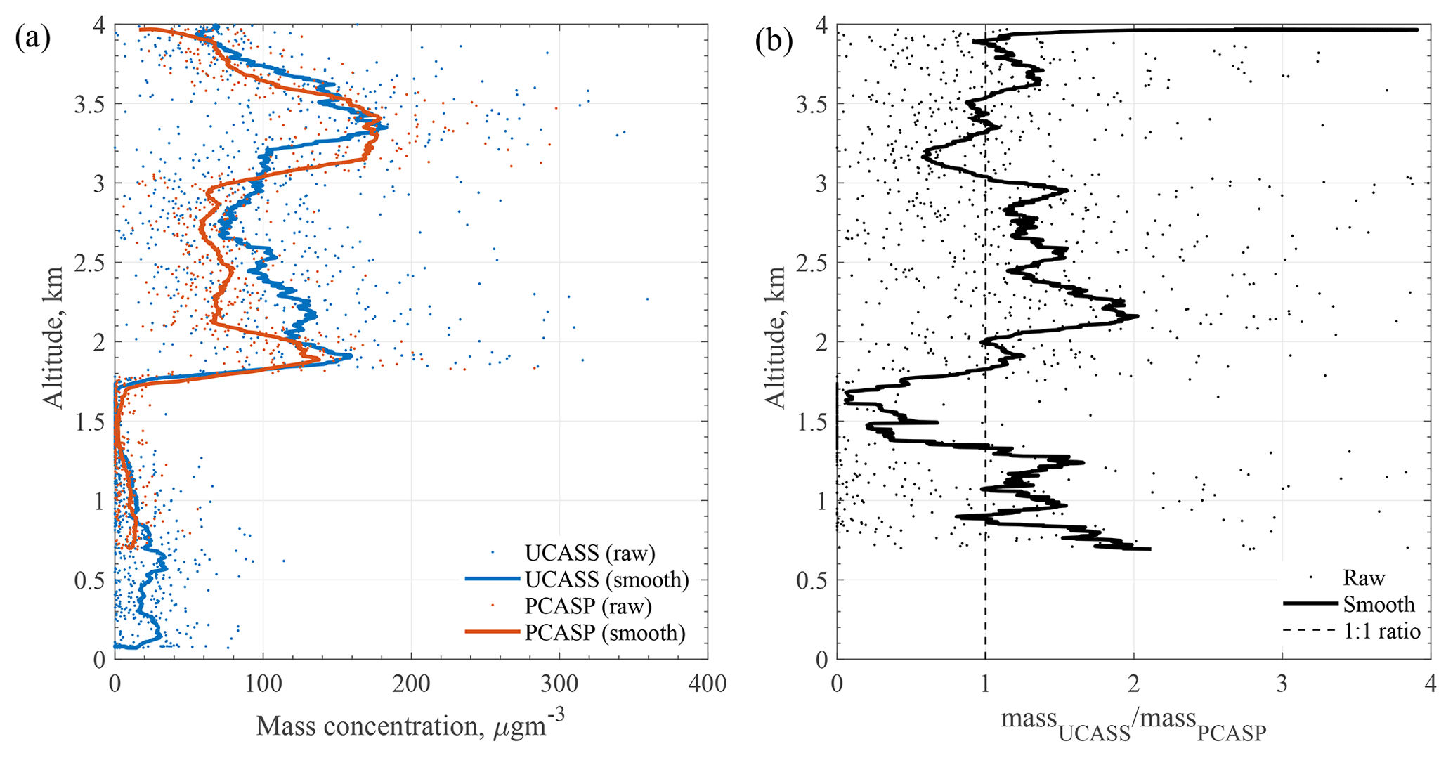
Figure 20Panel (a) shows the measured mass concentrations with respect to altitude for the balloon-borne UCASS (blue) and aircraft-mounted PCASP (orange). The raw data for each instrument are shown via individual data points, and the smoothed data are shown by a solid line, using a 10-point moving average. The mass concentrations shown pertain to particles within the 0.4–3 µm size range for comparative purposes. Panel (b) shows the ratio of the UCASS-measured mass concentration to the PCASP-measured mass concentration. It can be seen that the largest differences occur at the top and bottom of the dust layer, which may be due to spatial variation and/or gravitational settling.

Download