A geometry-dependent surface Lambertian-equivalent reflectivity product for UV–Vis retrievals – Part 2: Evaluation over open ocean

Fasnacht, Zachary; Vasilkov, Alexander; Haffner, David; Qin, Wenhan; Joiner, Joanna; Krotkov, Nickolay; Sayer, Andrew M.; Spurr, Robert

doi:https://doi.org/10.5194/amt-12-6749-2019

Articles | Volume 12, issue 12

https://doi.org/10.5194/amt-12-6749-2019

Articles | Volume 12, issue 12

Research article

19 Dec 2019

Research article |

| 19 Dec 2019

A geometry-dependent surface Lambertian-equivalent reflectivity product for UV–Vis retrievals – Part 2: Evaluation over open ocean

Zachary Fasnacht, Alexander Vasilkov, David Haffner, Wenhan Qin, Joanna Joiner, Nickolay Krotkov, Andrew M. Sayer, and Robert Spurr

Abstract

Satellite-based cloud, aerosol, and trace-gas retrievals from ultraviolet (UV) and visible (Vis) wavelengths depend on the accurate representation of surface reflectivity. Current UV and Vis retrieval algorithms typically use surface reflectivity climatologies that do not account for variation in satellite viewing geometry or surface roughness. The concept of geometry-dependent surface Lambertian-equivalent reflectivity (GLER) is implemented for water surfaces to account for surface anisotropy using a Case 1 water optical model and the Cox–Munk slope distribution for ocean surface roughness. GLER is compared with Lambertian-Equivalent reflectivity (LER) derived from the Ozone Monitoring Instrument (OMI) for clear scenes at 354, 388, 440, and 466 nm. We show that GLER compares well with the measured LER data over the open ocean and captures the directionality effects not accounted for in climatological LER databases. Small biases are seen when GLER and the OMI-derived LER are compared. GLER is biased low by up to 0.01–0.02 at Vis wavelengths and biased high by around 0.01 in the UV, particularly at 354 nm. Our evaluation shows that GLER is an improvement upon climatological LER databases as it compares well with OMI measurements and captures the directionality effects of surface reflectance.

Download & links

Article (PDF, 6052 KB)

How to cite

How to cite.

Dates

Received: 29 Jun 2019 – Discussion started: 22 Jul 2019 – Revised: 16 Oct 2019 – Accepted: 10 Nov 2019 – Published: 19 Dec 2019

1 Introduction

Satellite retrievals of clouds, aerosols, and trace gases rely on the accurate representation of surface reflectivity. Many modern satellite ultraviolet (UV) and visible (Vis) trace-gas algorithms use the mixed Lambertian-equivalent reflectivity (LER) model which assumes the measured top-of-atmosphere (TOA) radiance is a combination of the clear-sky and cloudy-sky radiances weighted by an effective cloud fraction (ECF) (Koelemeijer et al., 2001; Seftor et al., 1994; Stammes et al., 2008). While many databases of LER currently exist, they are typically climatological LER datasets based on the minimum or the mode of the LER distribution. Therefore, they do not account for the directionality effects due to the variation of satellite viewing and solar illumination geometries. Further, they do not capture day-to-day change in the roughness of the water surface due to changing wind speed which can impact surface reflectance. Additionally, climatological LER databases may be affected by residual aerosol and cloud contamination. These databases include Kleipool et al. (2008) using data from the Ozone Monitoring Instrument (OMI) for wavelengths 328–499 nm, Koelemeijer et al. (2003) from the Global Ozone Monitoring Experiment (GOME) for wavelengths 335–772 nm, and Tilstra et al. (2017) from GOME-2 for wavelengths between 335 and 772 nm.

The bidirectional reflectance distribution function (BRDF) describes the variations of the surface reflectivity for all illumination and viewing geometries. Given a specific solar and viewing angle from a satellite and the BRDF of the surface, a quantity known as the bidirectional reflectance factor (BRF) can be derived for that surface. BRF is defined as the ratio of the radiant flux reflected by a surface to the radiant flux reflected into the identical beam geometry by an ideal diffuse Lambertian surface, irradiated under the same conditions as the sample surface (Schaepman-Strub et al., 2006). A peak in the BRDF arises due to sunglint phenomena when the Sun and satellite viewing angles are similar and oriented in a forward scattering geometry. Sunglint is strongest for smooth water surfaces that permit nearly perfect Fresnel reflection of direct light from the ocean surface (Kay et al., 2009; Cox and Munk, 1954; Thomas and Stammes, 1999). Additionally, there is an increase in radiance near the outer edges of the satellite swath viewing geometry, when TOA radiances increase due to increased effects of Rayleigh scattering. The increase in diffuse sky reflection from the ocean surface becomes more significant at these longer path lengths, and the relative contributions from the water-leaving radiance to the intensity reaching the satellite is reduced (Vasilkov et al., 2017).

Vasilkov et al. (2017) introduced a concept known as geometry-dependent LER (GLER), where for a specific viewing geometry, TOA radiances are simulated over a non-Lambertian surface using the BRDF. GLER can be easily implemented into trace-gas algorithms by simply replacing the currently used LER climatologies. For Vis wavelengths, the change in surface reflectivity associated with the implementation of GLER was found to directly decrease the OMI NO₂ air mass factor (AMF) over land and oceans by as much as 15 % and change the OMI NO₂ AMF indirectly by an additional −22 % to 13 % through changes to retrieved cloud properties (Vasilkov et al., 2017). In the UV, Ahn et al. (2014) noted that unrealistic surface albedo is one of the main causes for uncertainty in aerosol retrievals, while Torres et al. (1998) reported that surface albedo errors can lead to as much as a 5 % error in retrieved aerosol optical depth (AOD) for weakly absorbing aerosols.

Qin et al. (2019) evaluated the OMI 466 nm GLER product over land generated using BRDF data from the Moderate Resolution Imaging Spectroradiometer (MODIS). They compared GLER with OMI-derived LER globally and found GLER was biased low by 0.01 to 0.02 relative to OMI. The difference was attributed to several factors, including small calibration differences between MODIS and OMI and possible residual cloud and/or aerosol contamination in the OMI data that was not completely filtered out.

Here we evaluate the GLER product generated for the OMI instrument for ocean scenes. OMI is a hyperspectral UV–Vis (270–500 nm) imager on board the NASA Aura satellite, which was launched in July 2004. The high spectral resolution (0.42–0.63 nm) of the UV (270–370 nm) and Vis (350–500 nm) channels enables retrievals of many important atmospheric constituents including O₃, NO₂, SO₂, and aerosols. OMI has a spatial resolution of 13 km × 24 km at nadir with a field of view (FOV) of 0.8^∘ in the flight direction and 115^∘ across the swath. Prior to 2008, OMI provided global coverage daily with a repeat cycle of 16 d. The OMI row anomaly affects data coverage starting in mid-2007 (Schenkeveld et al., 2017), but a substantial amount of high-quality global data remain available thereafter.

In this work we focus on evaluation of GLER at UV and Vis wavelengths over oceans. In the UV, 354 and 388 nm are chosen for evaluation as both are important in the OMI retrieval of aerosol properties (Torres et al., 2007), and additionally OMI Raman cloud retrievals are performed at 354 nm (Vasilkov et al., 2008). For Vis wavelengths, 440 and 466 nm are chosen as they are important for O₂–O₂ cloud retrievals (Vasilkov et al., 2018; Veefkind et al., 2016) as well as NO₂ retrievals (Krotkov et al., 2017; Lamsal et al., 2014).

Whereas the land product described in Qin et al. (2019) used a model of BRDF with input from MODIS, GLER for ocean scenes is produced solely by modeling of water-leaving radiance and surface reflection. These surface-leaving radiance contributions are geometry-dependent, and the anisotropic nature of light backscattered by the ocean has been studied in many papers (see, e.g., Gordon , 1989; Morel and Gentili, 1991, 1993, 1996; Park and Ruddick, 2005; Lee et al., 2013). For GLER, water-leaving radiance is simulated using a Case 1 water model (Morel, 1988; Morel and Maritorena, 2001) that depends only on chlorophyll concentration. This model is described in detail in Sect. 2.2. Reflection from the ocean surface is modeled using the Cox–Munk slope distribution (Cox and Munk, 1954) and is further described in Sect. 2.3.

The algorithms and approaches described in this paper are relevant to NASA's future Plankton, Aerosol, Cloud, ocean Ecosystem (PACE) mission. PACE is currently planned to launch in 2022–2023. Global PACE observations will provide data to monitor oceanic and atmospheric variables important for Earth's ecosystem, carbon cycle, and climate studies. The PACE Ocean Color Instrument (OCI) is designed as a wide-swath imaging spectrometer with a 1 km ground nadir resolution, a 5 nm spectral resolution between 345 and 890 nm, and several shortwave infrared bands (Werdell et al., 2019). As compared with the Sea-Viewing Wide Field-of-View Sensor (SeaWiFS), the Moderate resolution Imaging Spectrometer, and the Visible Infrared Imaging Radiometer Suite (VIIRS), the OCI will additionally measure TOA radiances in the UV to help identify phytoplankton composition and harmful algal blooms. PACE's spectral coverage from the UVA to green wavelength region and in the red to near-infrared will enable unparalleled evaluation of ocean ecosystem properties in optically complex waters and in regions of increasing eutrophication (Cetinic et al., 2018).

2 Data and methods

2.1 VLIDORT radiative transfer model

For radiative transfer calculations we use the Vector Linearized Discrete Ordinate Radiative Transfer (VLIDORT) model. VLIDORT is a multiple scattering radiative transfer model that can simulate Stokes vectors at any level in the atmosphere and for any scattering geometry with a Lambertian or non-Lambertian underlying surface (Spurr, 2006; Spurr and Christi, 2019). VLIDORT can simulate attenuation of solar and line-of-sight path radiances in a spherical atmosphere. In this study, we correct for the effects of atmospheric sphericity for both incoming solar and outgoing viewing directions based on a regular pseudospherical geometry calculation. This is important for large solar and viewing zenith angles. We also include polarization using the vector mode, because to neglect it can lead to considerable errors for modeling backscattered radiances in the UV–Vis wavelength range.

2.2 Water-leaving radiance implementation

VLIDORT has a supplement (VSLEAVE) for the generation of surface-leaving radiances for use as inputs to the main radiative transfer calculation in the atmosphere. This supplement can be used for either simulations of solar-induced fluorescence or water-leaving radiances from Case 1 waters. Our Case 1 water model accounts for the bidirectional effects following Morel and Gentili (1996). In this paper we do not account for vibrational Raman scattering in ocean water (Morel et al., 2002; Vasilkov et al., 2002). The common Case 1 water model developed for the Vis (Morel, 1988) was extended to the UV using a parameterization of the particulate matter absorption coefficient from Vasilkov et al. (2002, 2005). The model requires as input several quantities that affect absorption and scattering properties of seawater and its constituents. Extinction coefficients for water absorption are taken from Lee et al. (2015), chlorophyll absorption coefficients from Vasilkov et al. (2005) below 400 nm and Lee et al. (2005) at longer wavelengths, and colored dissolved organic matter (CDOM) absorption from Morel and Maritorena (2001). The water scattering coefficients we use are from Morel et al. (2007), and those for chlorophyll scattering are from Morel and Maritorena (2001). A detailed description of these parameterizations is provided in Appendix A2.

The computation of emerging water-leaving radiance L_w depends not only on the optical properties of marine constituents and radiative processes in the near-surface ocean, but also on the total atmospheric direct and diffuse downwelling transmittance T_atm of atmospheric light through the air–water interface. This complicates separation of the water-leaving calculation and the calculation of atmospheric radiance propagation. Additionally, T_atm will in general depend on the surface-leaving contribution and hence on marine constituents. VLIDORT and its supplement VSLEAVE are therefore coupled. This coupling can be treated formally with a coupled ocean–atmosphere radiative transfer model such as that described in Spurr et al. (2007). Here, however, we have developed a simple coupling scheme for VLIDORT that ensures the value of L_w used as a input at the ocean surface will correspond to the correct value of the downwelling flux reaching the surface interface. The first applications of this new water-leaving model were presented in Vasilkov et al. (2017) and Sayer et al. (2017). The coupled model approach is described further in Appendix B.

2.3 Cox–Munk BRDF implementation

A supplement (VBRDF) is implemented in VLIDORT to account for the reflection of the water surface using the Cox–Munk slope distribution (Cox and Munk, 1954). We use the full form of the Cox–Munk distribution in which the facet slope variance depends on both wind speed and wind direction. Polarization at the ocean surface is accounted for using a full Fresnel reflection matrix as suggested by Mishchenko and Travis (1997). Additionally we account for contributions from oceanic foam that can be significant for high wind speeds using work by Frouin et al. (1996).

2.4 Ancillary data for water model

As mentioned in the introduction, modeling of the water-leaving radiance requires information on the chlorophyll concentration, and the modeling of Cox–Munk surface roughness depends on wind speed and wind direction. These inputs are not available directly from the OMI satellite and so other sources of ancillary inputs are required.

The wind speed measurements for GLER come from a pair of satellite microwave imagers. The first is the Advanced Microwave Scanning Radiometer – Earth Observing System (AMSR-E) instrument on board the NASA Aqua satellite with a spatial resolution of 0.25^∘ (Wentz and Meissner, 2004). The AMSR-E instrument, however, ceased operations in October 2011 due to an issue with the spinning mechanism (Wentz and Meissner, 2007). After October 2011, data are taken from the Special Microwave Imager/Sounder (SSMIS) with a spatial resolution of 0.25^∘. SSMIS is on board the Air Force Defense Meteorological Satellite Program (DMSP) satellite F16 (Wentz et al., 2012). While the SSMIS instrument has been operating since October 2003, the AMSR-E instrument was chosen for the first half of the OMI mission due to the small difference in Equator crossing times of 7–15 min between the Aqua and Aura satellites, whereas the F16 satellite crossing times range from 6 h behind Aura in 2005 to 2 h behind Aura currently. In future work, we plan to replace the SSMIS F16 wind speed with the AMSR-2 wind speed data. AMSR-2 is on board the Global Change Observation Mission Water Satellite 1 (GCOM-W1), which has an Equator crossing time more similar to OMI (Imaoka et al., 2012). Gaps in the wind speed data due to extreme glint or rain are filled by the Global Modeling Assimilation Office (GMAO) Goddard Earth Observing System Model Forward Processing for Instrument Teams (GEOS-5 FP-IT) near-real-time assimilation with a spatial resolution of 0.625^∘ longitude by 0.5^∘ latitude and a temporal resolution of 3 h (Lucchesi, 2013). Wind direction data are also from the GEOS-5 FP-IT model.

Monthly chlorophyll data from the MODIS instrument, which is on board the NASA Aqua satellite, were used in modeling of the water-leaving radiance (Hu et al., 2012). These chlorophyll data have a spatial resolution of 4 km. The MODIS daily chlorophyll data are not used due to large gaps caused by clouds and aerosols. Some gaps still exist in the monthly data and are filled by other datasets from the MODIS team. These include monthly climatological and yearly chlorophyll datasets which are also at a 4 km resolution. The benefit of using the monthly chlorophyll data instead of the climatological data comes from the ability to capture interannual trends due to phenomena such as the El Niño–Southern Oscillation (ENSO).

2.5 Calculation of LER and GLER

Using the equation from Dave (1978), LER (R) can be calculated from TOA radiance (I_comp) by inverting the following:

\begin{matrix} (1) & \begin{aligned} I_{comp} & (λ, θ, θ_{0}, ϕ, P_{s}, {BRF}_{s}) = I_{0} (λ, θ, θ_{0}, ϕ, P_{s}) \\ + \frac{R T (λ, θ, θ_{0}, P_{s})}{1 - R S_{b} (λ, P_{s})}, \end{aligned} \end{matrix}

where λ is wavelength; θ is the viewing zenith angle (VZA); θ₀ is the solar zenith angle (SZA); ϕ is the relative azimuth angle (RAA); P_s is the surface pressure; I₀ is the path scattering radiance by the atmosphere, calculated as the TOA radiance for a black surface; T is total (direct + diffuse) solar irradiance reaching the surface and reflected back to the satellite, multiplied by the transmittance; S_b is the diffuse flux reflectivity of the atmosphere; and R is LER.

In order to calculate GLER, we use VLIDORT to simulate I_comp for a clear sky over a non-Lambertian surface with the water-leaving radiance model described in Sect. 2.2 along with the Cox–Munk slope distribution for surface roughness. A lookup table (LUT) approach is used to calculate TOA radiance operationally, as running VLIDORT can be computationally expensive. Details on the LUT approach can be found in Appendix C. Given TOA radiance from VLIDORT, we can then calculate GLER using Eq. (1).

2.6 OMI data and selection criteria

The measured LER data used to evaluate ocean GLER in this study were retrieved from OMI Collection 3 Level 1b Vis channel radiance data by inverting Eq. (1) where I_obs is used in place of I_comp. The OMI radiances are normalized using the OMI day-1 solar irradiance spectrum adjusted for variation in Earth–Sun distance when radiance measurements were collected. The GLER product is designed to characterize the magnitude and the angular variability of the Earth's surface reflectance in a Rayleigh atmosphere, and therefore several aspects of instrument calibration must be considered. The absolute radiometric calibration error will introduce bias and inconsistency across the measurement swath for LER at any single wavelength. Dobber et al. (2008) estimated that the uncertainty in radiometric calibration of OMI Collection 3 Sun-normalized radiances is under 2 % and that the relative viewing angle dependence is also less than 2 %. Schenkeveld et al. (2017) evaluated long-term changes in the absolute radiometric response of the OMI instrument and estimated degradation of approximately 1 %–1.5 % per decade in the wavelength region used in this study. Since we compare results at 354, 388, 440, and 466 nm in this study, the spectral dependence of the OMI calibration is also an important consideration. Little work has been published on this topic, although the study by Jaross and Warner (2008) compared the OMI Sun-normalized radiances to radiative transfer model simulations over Antarctic ice and showed that the spectral dependence of the OMI calibration is within the absolute radiometric uncertainty.

Beginning in mid-2007, OMI experienced an anomaly known as the “row anomaly” that has affected the L1b radiance data. There have been several impacts from the row anomaly including decreased radiances due to possible blockage, increased signal due to sunlight being reflected into the instrument, a wavelength shift due to a change in the slit function, and earthshine radiances from outside the FOV that are reflected into the nadir port. The row anomaly is further explained in Schenkeveld et al. (2017). For this reason, after 2007 we focus only on rows 1–21, which are not affected by the row anomaly.

Absorption by O₂–O₂ and O₃ were accounted for at 440 and 466 nm but neglected for 354 and 388 nm. Since GLERs were simulated for a Rayleigh-only atmosphere, pixels with absorbing aerosols are removed using the OMAERUV absorbing aerosol index AI ( $| AI | > 0.5$ are removed) (Torres et al., 2007). We compare the evaluation for two independent cloud screening methods to determine which will better represent the GLER evaluation. The MODIS geometrical cloud fraction (GCF) is retrieved from the 15 µm CO₂ absorption region (Menzel et al., 2007) and is colocated to the OMI FOV in the OMMYDCLD product (Joiner, 2014). The OMI Raman cloud product contains cloud pressure based on rotational Raman scattering and ECF calculated at 354 nm using the Cox–Munk distribution to model ocean surface reflectivity (Vasilkov et al., 2008).

We compare cases with and without sunglint separately because the reflection of light in each case is quite different. For comparisons excluding sunglint scenes, we screen out data with a sunglint angle of less than 20^∘ in which sunglint can occur. For the comparisons with sunglint, while the sunglint angle of 20^∘ is again used to choose the sunglint region, additional screening based on the spectral dependence of the measured LER is performed to remove clouds within the sunglint region. The reason for this is that cloud fraction retrievals are affected by sunglint. The difference in LER occurs because of a spectrally dependent error in the underestimation of the Rayleigh scattering of diffuse light when one assumes a Lambertian ocean surface, when the reflectance is in fact specular. We select sunglint scenes when the difference between the measured LER at 354 and 388 nm is less than −0.05. We note that some weaker sunglint has an LER difference that is not below this threshold, but here we focus on stronger glint that has no cloud contamination.

In addition to the OMI-derived LER, we compare with the Kleipool LER climatology (Kleipool et al., 2008), since a number of current operational algorithms use these LER data as input. There are two LER datasets available from the Kleipool data, one representing the monthly minimum LER and another determined through interpretation of LER histograms. Both are shown in our evaluation as each is used in some algorithms.

3 Results and discussion

3.1 Global comparison of GLER and OMI-derived LER

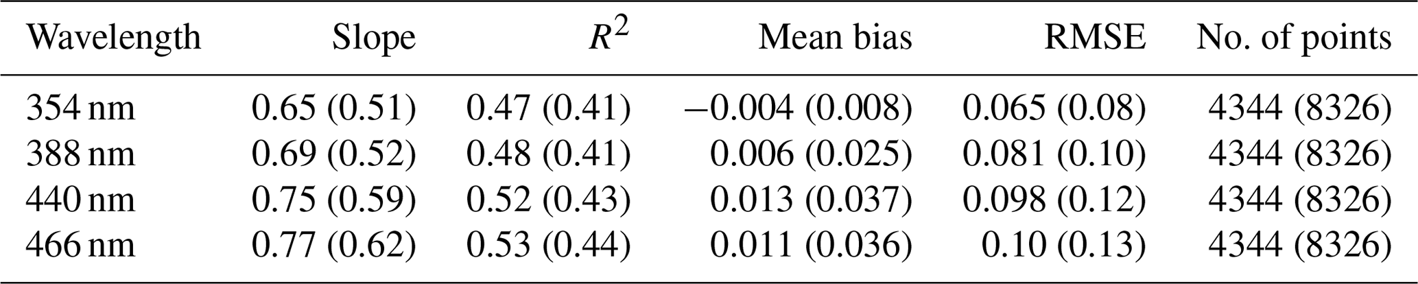
First we compare GLER with the OMI-derived LER globally for January and July 2006 at four wavelengths in Figs. 1 and 2. To determine a cloud screening method for the evaluation of sunglint-free data, in Fig. 1 we compare GLER with the OMI-derived LER using the cloud screening methods introduced in Sect. 2.6. We note there is a spectral dependence in the difference between GLER and the OMI-derived LER. At 354 nm, GLER is biased high compared to the OMI-derived LER, whereas no bias exists at 388 nm. For longer wavelengths of 440 and 446 nm, GLER is biased low compared to the OMI-derived LER. As shown in Table 2, the GLER and the OMI-derived LER compare best in January at 388 nm where R² is 0.76 and the bias is 0.002 with the Raman-based ECF (using the MODIS GCF R² is 0.60 and the bias is 0.007).

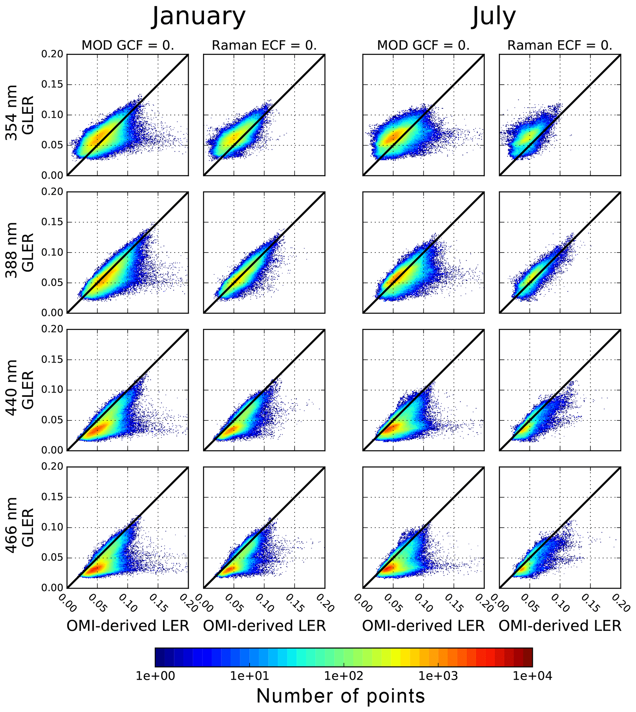
https://www.atmos-meas-tech.net/12/6749/2019/amt-12-6749-2019-f01

Figure 1Scatterplots of OMI-derived LER vs. GLER for two months in 2006 (January on left and July on right) with possible sunglint removed at four wavelengths (354, 388, 440, and 466 nm). Data are for deep ocean (based on OMI Level 1b ground pixel quality flags) and have been screened for aerosols (OMAERUV |AI| < 0.5). Clouds are screened through two different methods which are described in Sect. 2.6. Only data with a solar zenith angle less than 70^∘ are included as cloud shadowing at high view angles can decrease the OMI-derived LER.

Download

https://www.atmos-meas-tech.net/12/6749/2019/amt-12-6749-2019-f02

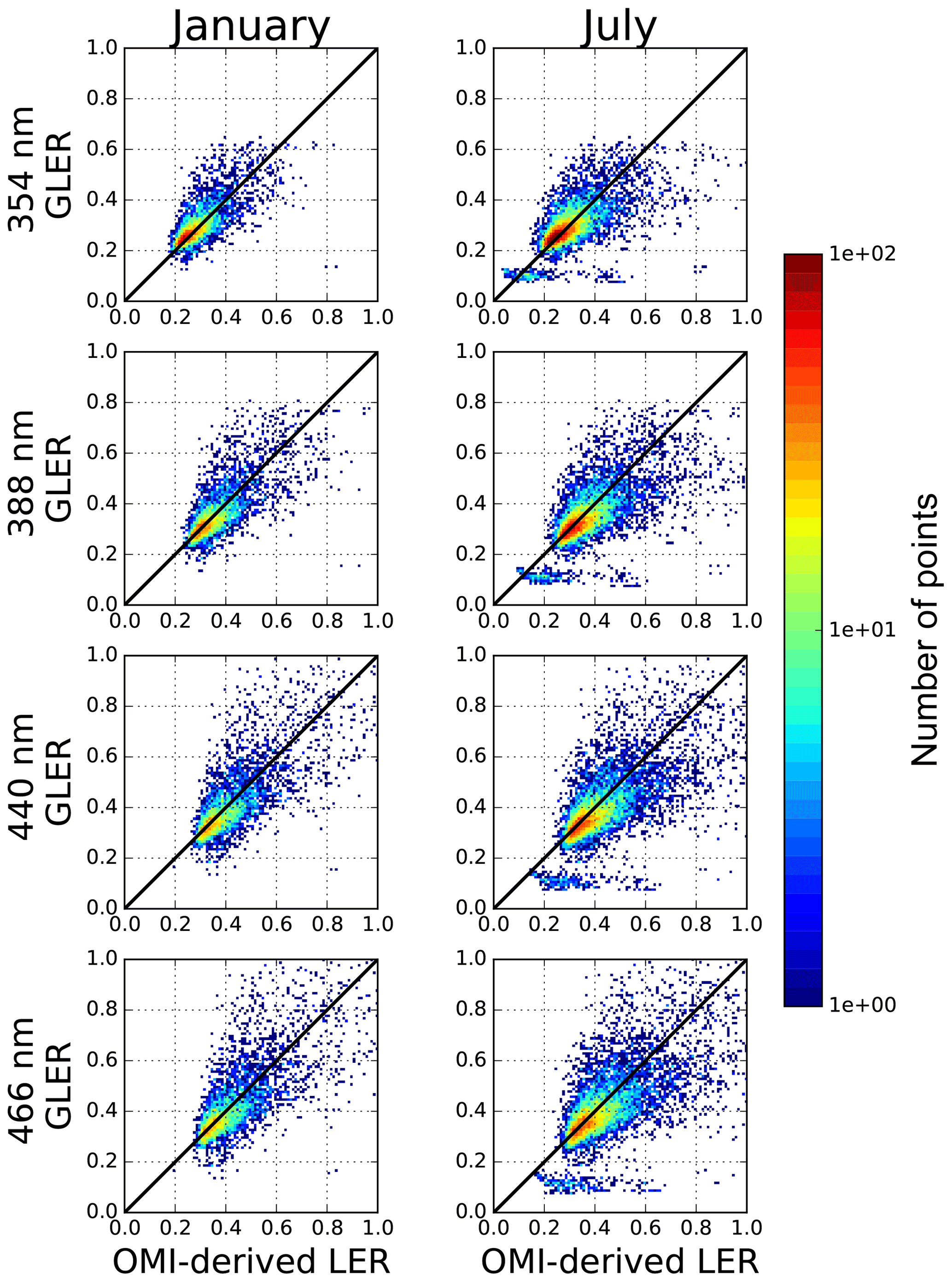
Figure 2Scatterplots of OMI-derived LER vs. GLER for two months in 2006 (January on left and July on right) for pixels with sunglint at four wavelengths (354, 388, 440, and 466 nm). Data are for deep ocean with no screening for clouds or aerosols.

Download

Overall the comparison is better when using the Raman-based ECF cloud screen than when using the MODIS GCF. This is expected given that there is a 15 min window between the Aqua and Aura overpass times in 2006 (becomes 7 min in 2009) leading to some change in cloud cover. It is also worth noting, since OMI has a wider swath than MODIS, cloud retrievals are not available from MODIS for pixels on the edge of OMI swath (these pixels are not shown in Fig. 1). For these reasons the Raman-based ECF will be used for cloud screening in the rest of the paper.

In Fig. 2, the comparisons of GLER and OMI-derived LER are presented for data with sunglint. These data were not screened with cloud or aerosol retrievals, as strong glint can lead to artificial classification of aerosol or clouds in the retrieval algorithms. As shown in Table 3, the bias between GLER and the OMI-derived LER is smaller for the data with sunglint than the sunglint-free data. For sunglint pixels, the bias is smaller at UV wavelengths where the water-leaving radiance contributes the least. For the brighter glint data, there is much more uncertainty and GLER is biased high compared with the OMI-derived LER. If the measured wind speed is too low, the model will overestimate the LER of the glint, whereas when the measured wind speed is too high, the model will underestimate the LER of glint. This sensitivity to the wind speed will be further evaluated in Sect. 3.5. The small bias is possibly caused by aerosols which scatter or absorb the direct light causing a small dimming effect in the OMI glint data. This issue will be evaluated in Sect. 3.3.

Table 1Statistical analysis of GLER vs. OMI LER for nonsunglint scenes. January (July) 2006 deep ocean only with Raman-based ECF = 0.0 (corresponds to the second and fourth column of Fig. 1).

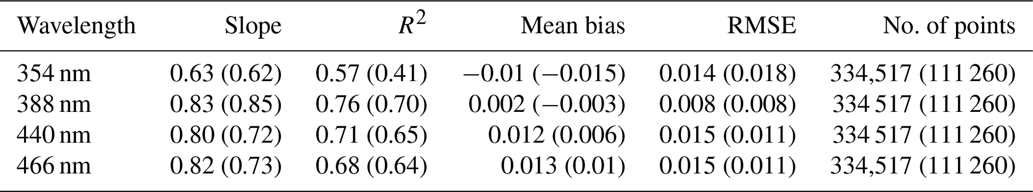
Download Print Version | Download XLSX

Table 2Statistical analysis of GLER vs. OMI LER for nonsunglint scenes. January (July) 2006 deep ocean only with MODIS GCF = 0.0 (corresponds to the first and third column of Fig. 1).

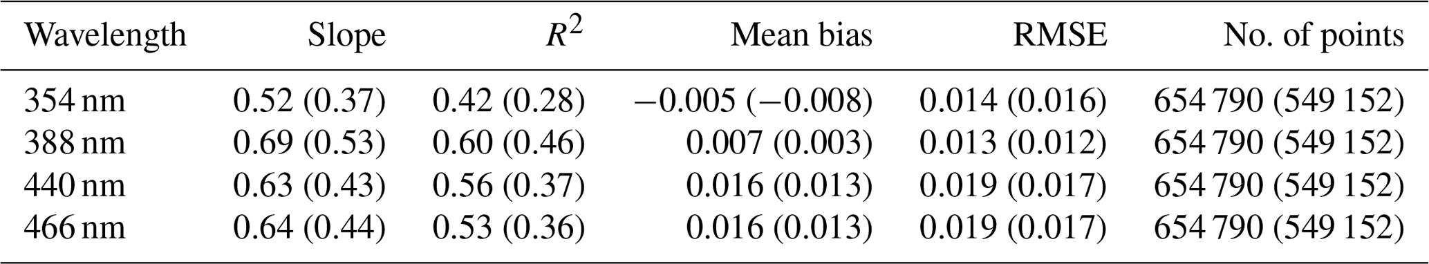
Download Print Version | Download XLSX

Table 3Statistical analysis of GLER vs. OMI LER for sunglint-only scenes. January (July) 2006 deep ocean only.

Download Print Version | Download XLSX

3.2 Angular behavior of GLER

Figures 3 and 4 show a comparison of the cross-track dependence of GLER and OMI-derived LER along with the Kleipool LER climatology for a few solar zenith angle ranges screened for clouds using the Raman-based ECF and screened for absorbing aerosols with the OMAERUV AI. GLER follows a similar cross-track pattern at various solar zenith angles to the OMI-derived LER that varies with wavelength. However, there is a bias between GLER and the OMI-derived LER which varies by wavelength. For Vis wavelengths, the OMI-derived LERs are biased high by as much as 0.01–0.02 compared to the GLER, whereas for UV wavelengths the bias is nearly zero at 388 nm and at 354 nm GLER is biased around 0.01 higher than the OMI measurements. In the UV channels, especially at 354 nm, the bias varies both with cross-track and solar zenith angle.

https://www.atmos-meas-tech.net/12/6749/2019/amt-12-6749-2019-f03

Figure 3January 2006 LER as a function of VZA for select SZA ranges at 354 and 388 nm over the Pacific Ocean (only deep ocean pixels considered). The blue error bars represent the 2 % calibration uncertainty of OMI (Dobber et al., 2008). Negative VZAs represent the west side of the OMI swath (forward scattering), whereas positive VZAs represent the east side of the OMI swath (backward scattering). Data are screened for clouds with the Raman-based ECF and aerosols are removed with the OMAERUV AI.

Download

https://www.atmos-meas-tech.net/12/6749/2019/amt-12-6749-2019-f04

Figure 4Same as Fig. 3 but for 440 and 466 nm.

Download

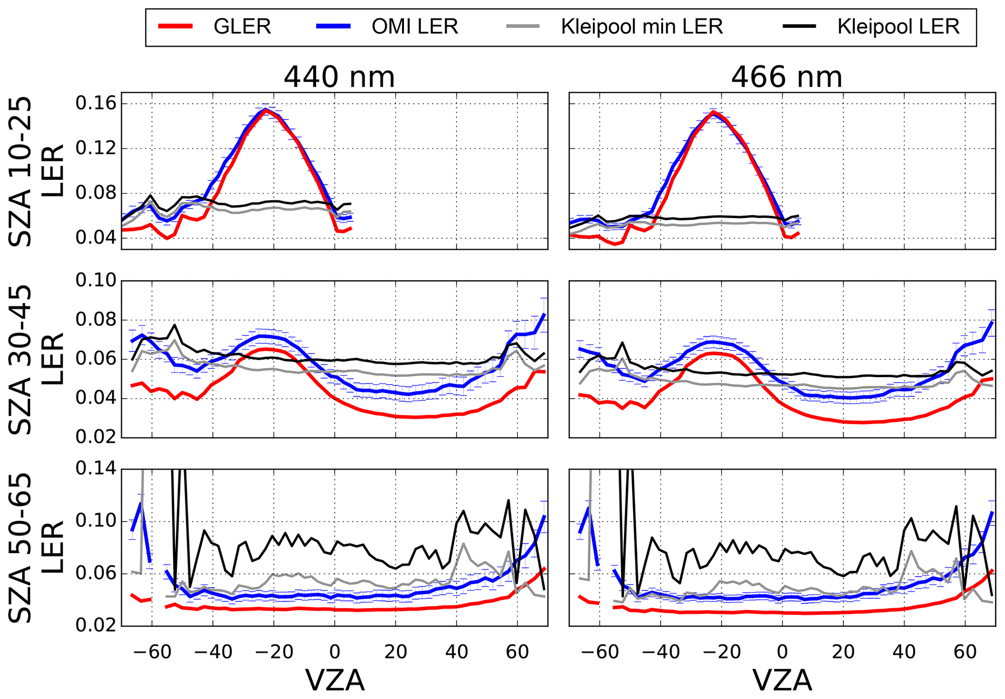
The Kleipool LER climatology compares well with the OMI-derived LER near nadir but does not capture any of the BRDF effects seen in both GLER and OMI-derived LER since it is a climatology that averages all viewing geometries. We note that there is a slight increase in Kleipool LER at higher viewing zenith angles, but this is simply due to the sampling used for this analysis. Compared to the OMI-derived LER, the Kleipool data have a cross-track-dependent difference of as much as 0.04 outside of the sunglint and 0.1 in the sunglint for UV wavelengths. The difference between Kleipool and the OMI-derived LER (0.01) is smaller for Vis wavelengths outside of the sunglint. At the higher solar zenith angles, the Kleipool monthly data appear to be adversely affected either by ice or residual cloud that was not fully removed from the Kleipool LER climatology. This is evident by the large bias compared with OMI-derived LER as well as the large variability coming from spatial sampling.

3.3 Simulating GLER with aerosols

As noted in earlier sections, aerosols can have an impact on measured LER. For this reason, a simulation was performed to calculate GLER including the effect of aerosols. Aerosol-related input parameters to VLIDORT (layer AOD; single scattering albedo, SSA; and scattering matrix) are from MERRA-2 aerosol reanalysis data which are produced using the GEOS-5 atmospheric model and data assimilation system. MERRA-2 assimilates radiance data from a variety of satellite sensors which are then used to train a neural network to produce AOD which is calibrated to the Aerosol Robotic Network (AERONET) direct-Sun point measurements (Randles et al., 2017; Gelaro et al., 2017). The species-specific aerosol scattering matrices are characterized by six sets of matrix elements generated from the Mie theory.

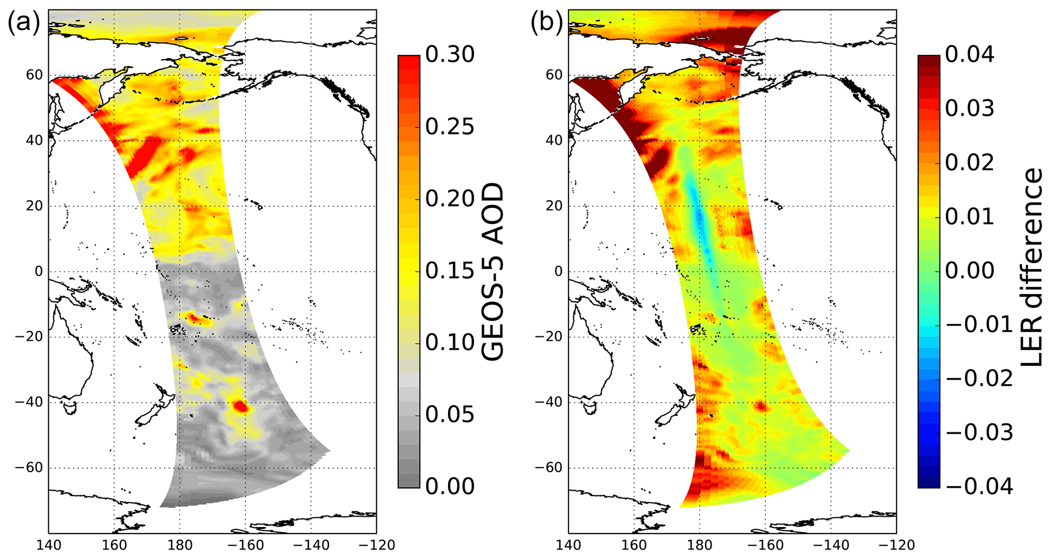
https://www.atmos-meas-tech.net/12/6749/2019/amt-12-6749-2019-f05

Figure 5Map showing the results from GLER aerosol simulation on 10 April 2006 for orbit 9229. Panel (a) is GEOS-5 470 nm AOD used in the simulation and panel (b) is change in GLER when the aerosol contribution is added to the simulations at 466 nm.

Download

https://www.atmos-meas-tech.net/12/6749/2019/amt-12-6749-2019-f06

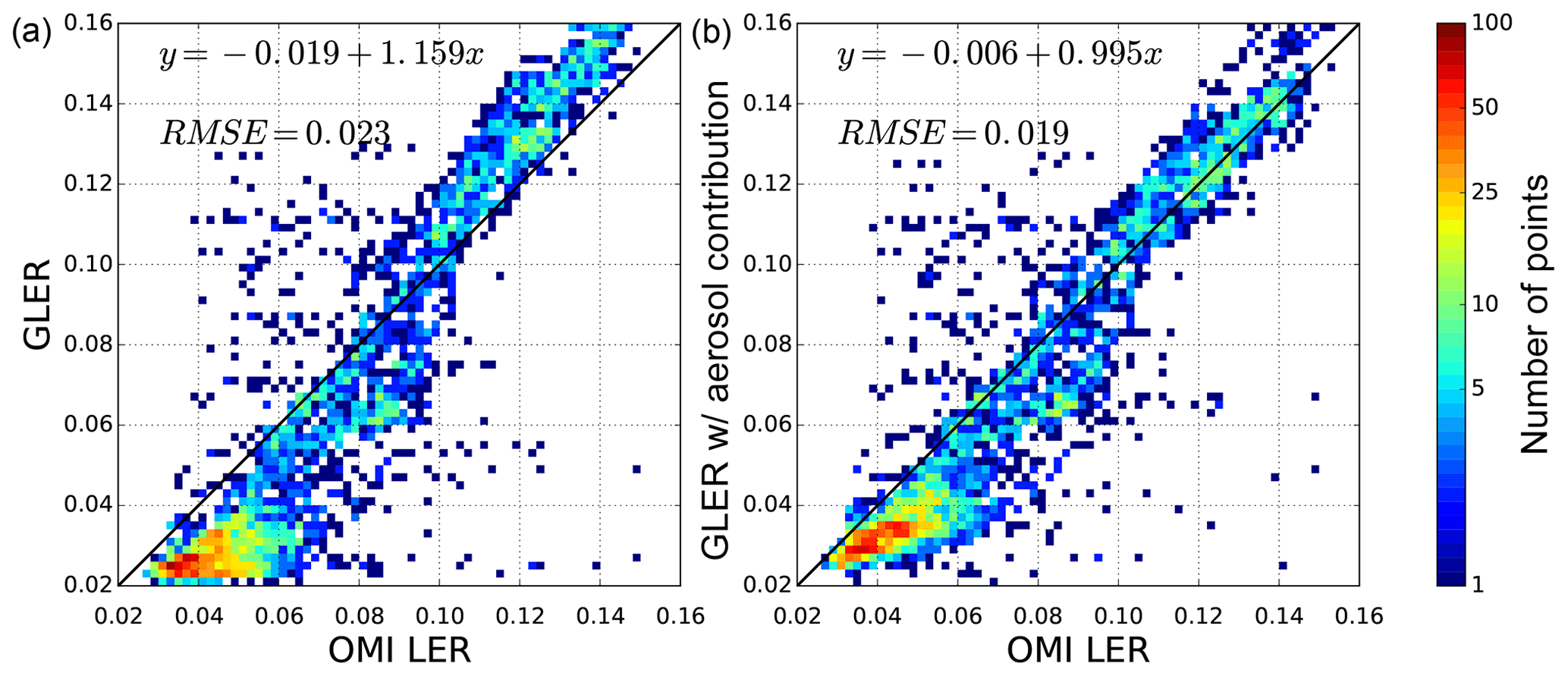
Figure 6Comparison of GLER versus OMI-derived LER for orbits on 10 April 2006 over the Pacific Ocean. Panel (a) is GLER compared to the OMI-derived LER at 466 nm, whereas panel (b) is GLER with contribution from aerosols vs. OMI-derived LER for 466 nm. All data are filtered to remove clouds with the Raman-based ECF.

Download

The simulation was performed for 10 April 2006 over the central Pacific Ocean in order to determine the aerosol effect for a general background oceanic aerosol case. Figure 5 shows the MERRA-2 AOD and the LER change due to added aerosols for orbit 9229 where AOD ranges from around 0.05 in the South Pacific Gyre to larger than 0.4 in the northern Pacific. The impact of the aerosols on GLER ranges from a decrease in LER of 0.01 in sunglint to an increase in LER of greater than 0.04 outside of the glint, especially at higher viewing angles. Figures 6 and 7 show the comparison between GLER and the OMI-derived LER as well as a comparison between GLER with a contribution from aerosols and the OMI-derived LER.

In Fig. 6 the addition of aerosols at 466 nm increases the LER by about 0.01 over darker surfaces, whereas the brighter regions which have some sunglint contribution show a reduction in LER of around 0.01. The combination of these changes improves the regression slope from 1.16 before considering aerosols at 466 nm to 1.0 after aerosols are introduced. After accounting for aerosols, OMI-derived LER is still around 0.01 higher than GLER at 466 nm for darker surfaces. The brighter surfaces, however, which have some sunglint contribution, have little to no bias after accounting for aerosols. Figure 8 shows that aerosols increase GLER generally by 0.01–0.02, with the largest increase at large forward scattering viewing zenith angles.

https://www.atmos-meas-tech.net/12/6749/2019/amt-12-6749-2019-f07

Figure 7Same as Fig. 6 but for 354 nm.

Download

https://www.atmos-meas-tech.net/12/6749/2019/amt-12-6749-2019-f08

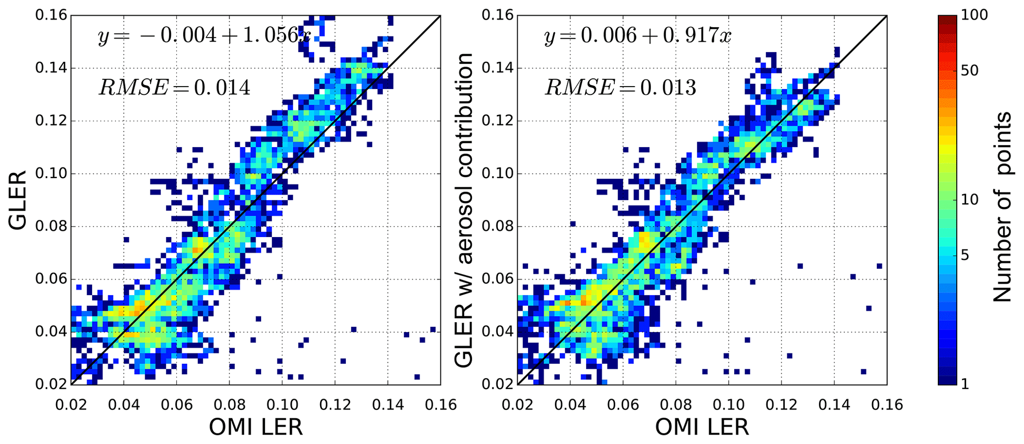
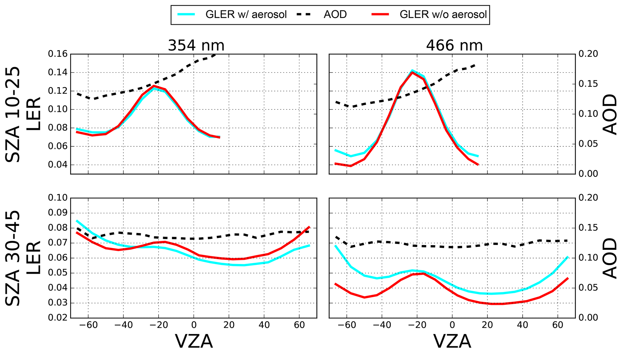
Figure 8LER as a function of VZA at 354 and 466 nm for orbits on 10 April 2006 over the Pacific Ocean. As in Fig. 3 negative VZAs represent the west side of the OMI swath whereas positive VZAs represent the east side of the OMI swath. Since only simulated data are shown, no cloud or aerosol screening is performed.

Download

At 354 nm the aerosol impact is not as significant as that seen for 466 nm with little to no change in the bias for darker surfaces and a reduction of around 0.01 for the brighter surfaces. In Fig. 8 there is a cross-track dependence in the aerosol contribution to GLER at 354 nm. For geometries with forward scattering (negative VZAs), the aerosol contribution can effectively increase the derived LER by 0.01 or more, whereas for backward scattering geometries (positive VZA) there is a small decrease in LER. This view angle dependence of the aerosol impact would remove the view-angle-dependent bias between GLER and OMI-derived LER seen in Fig. 3. Therefore, applying the aerosol impact to Fig. 3 would result in GLER being approximately 0.01 higher than the OMI-derived LER at 354 nm for all view angles.

In this case study, we note that an AOD of 0.1–0.15 increased the LER by as much as 0.01–0.02 at 466 nm, with the largest increase being in the forward scattering direction. At 354 nm, however, similar AOD values slightly decrease LER in the backward scatter direction but can increase LER by as much as 0.01 in the forward scattering direction. While this analysis was for only a specific case study, we note that the aerosol contribution likely accounts for some of the difference between GLER and the OMI-derived LER.

3.4 Interannual variability of LER

Surface LER over the ocean can change day to day with the chlorophyll concentration affecting the water-leaving radiance contribution and changes in the wind speed altering the roughness of the water surface. There is also a seasonal variation in LER due to the changing viewing geometry of satellite measurements as the SZA changes through the year. In Figs. 9 and 10, GLER and OMI-derived LER are shown for the duration of the OMI mission to evaluate the ability of GLER to capture these variations. In this figure, data were selected for a region in the South Pacific Gyre (180–120^∘ W, 30^∘ S–Equator) as this region is generally free of strong aerosols and has relatively low cloud fractions. OMI row 10 is evaluated to avoid sunglint as well as to avoid the OMI row anomaly which impacts many of the OMI rows starting around 2007 (Levelt et al., 2018; Schenkeveld et al., 2017). While this relatively small bias between GLER and the OMI-derived LER is evident, GLER does follow the same general trend as the OMI measured data.

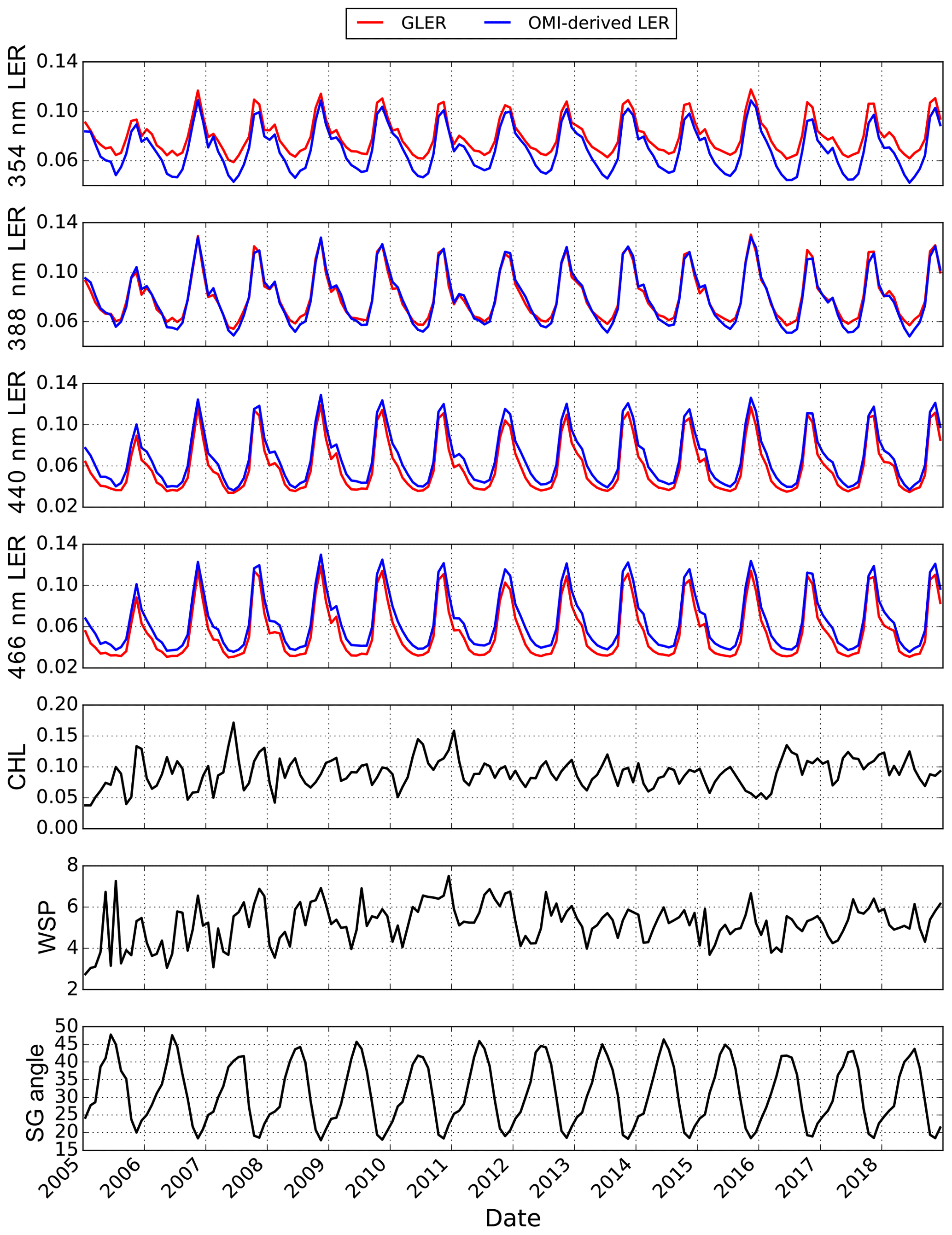
https://www.atmos-meas-tech.net/12/6749/2019/amt-12-6749-2019-f09

Figure 9Monthly mean of GLER and OMI-derived LER in the equatorial Pacific Ocean (180–120^∘ W, 30^∘ S–0) for four wavelengths (354, 388, 440, and 466 nm) as a function of time for the OMI mission from row 10. Corresponding chlorophyll and wind speed measurements along with sunglint angle used for GLER are shown in the bottom three panels. Data are filtered to remove clouds with the Raman-based ECF.

Download

https://www.atmos-meas-tech.net/12/6749/2019/amt-12-6749-2019-f10

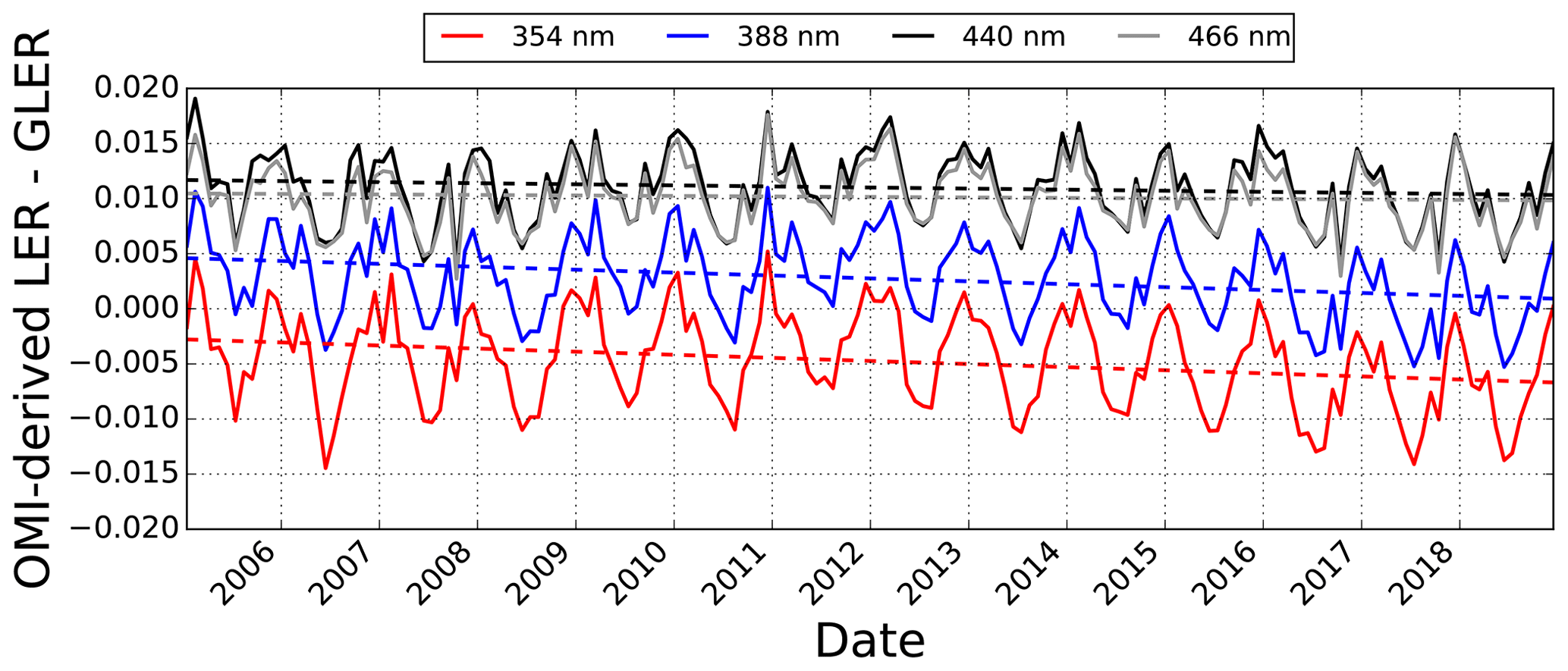
Figure 10Trend in the difference between the monthly mean GLER and the OMI-derived LER for the same location as in Fig. 9 at UV and Vis wavelengths for row 10. Data are filtered to remove clouds with the Raman-based ECF.

Download

Figure 10 shows there is about a 0.01 seasonal variation in the GLER and OMI-derived LER difference for all wavelengths which could possibly be due to seasonal changes in aerosols or seasonality in cirrus clouds that are too thin to be retrieved by the Raman-based ECF. We note that in Fig. 10 there is a small downward trend in the difference between GLER and OMI-derived LER of at most 0.005 in LER. At 354 nm a change of 0.005 LER corresponds to approximately 1 % TOA radiance, which is close to the 1 %–1.5 % TOA radiance degradation noted by Schenkeveld et al. (2017).

3.5 Sensitivity to chlorophyll and wind speed

Table 4Sensitivity to wind speed.

Download Print Version | Download XLSX

Table 5Sensitivity to chlorophyll.

Download Print Version | Download XLSX

Table 6Sensitivity to wind speed and chlorophyll.

Download Print Version | Download XLSX

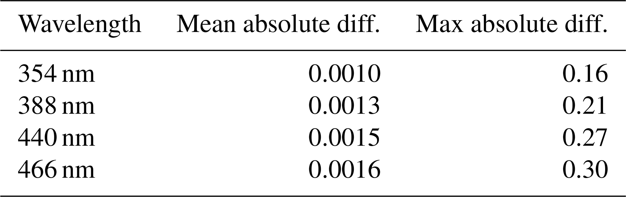
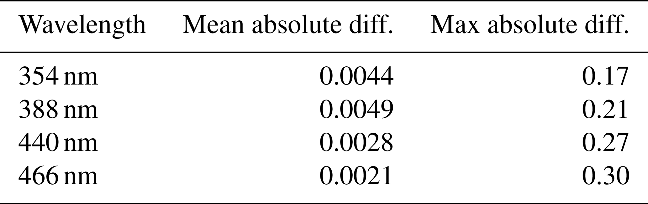
In order to determine the uncertainty in GLER calculations, a sensitivity test was performed based on the inputs of chlorophyll and wind speed. The wind speed measurements were perturbed ±1 m s⁻¹ as Wentz and Meissner (2000) note that is the uncertainty in their wind speed algorithm. The MODIS Ocean Color Team notes that the chlorophyll uncertainty varies regionally but can possibly be as high as 35 % (Moore et al., 2009). We perturb chlorophyll by this 35 % in order to gather an absolute bound of GLER to the chlorophyll input. We place an absolute lower bound on the wind speed in our calculations of 0.4 m s⁻¹ and a lower bound of 0.01 of milligrams per cubic meter (mg m⁻³) on the chlorophyll datasets as measurements of these input below these lower bounds are unrealistic and could lead to large errors in calculation of GLER. In Tables 4, 5, and 6 the magnitudes of the mean and max differences are reported in units of LER.

As seen in Table 4 the average wind speed sensitivity is quite small at around 0.0015, but the maximum sensitivity can become as high as 0.3 due to the high sensitivity of sunglint to wind speed. This is because for extreme sunglint cases a small roughness in the ocean surface will lead to increased scattering of light which will significantly diminish the strength of the glint. It is worth noting that while such roughness decreases the strength of the glint, it will increase the overall size of the region affected by sunglint due to the scattering of light at the ocean surface. The wind speed sensitivity decreases with decreasing wavelength because the fraction of the direct solar light which is responsible for sunglint decreases for shorter wavelengths where the contribution of the diffuse light increases due to Rayleigh scattering.

In Table 5 the chlorophyll sensitivity is shown to be much smaller than the wind speed sensitivity. In contrast with the wind speed sensitivity, the chlorophyll sensitivity is largest at UV wavelengths because the CDOM absorption, which rises with increasing chlorophyll according to the Case 1 water model, exponentially increases for shorter wavelengths.

To determine the combined effect, we additionally calculated GLER perturbing both the wind speed and chlorophyll for the four possible combinations. Table 6 shows the mean difference from the combined sensitivity analysis in GLER is similar to that obtained by only perturbing the chlorophyll. The maximum difference from the combined sensitivity test, however, is similar to that of the wind speed perturbation. This is because while the wind speed has a significant impact on sunglint, only a small fraction of OMI pixels are impacted by glint.

3.6 Additional sources of uncertainty

We note that, in addition to the sensitivities from the input data, uncertainties also result from the modeling of the GLER as well as the OMI data used for the evaluation. One possible source of uncertainty is the water-leaving radiance model being used in the calculations. Here we implement a Case 1 water model that is assumed to be representative of the global oceans with dependence only on chlorophyll. Szeto et al. (2011), however, showed that the world's oceans are optically variable and that optical parameters such as chlorophyll absorption vary even for Case 1 open ocean. Work by Lee et al. (2006) similarly showed that large deviations exist from the presumed Case 1 water model due to uncertainty in the optical properties used to parameterize the models. They determined that the SeaWiFS remote sensing reflectance retrievals at 555 nm for Case 1 water have a deviation of ±50 % from that of a Case 1 bio-optical property model.

Our simulations do not include any vibrational Raman scattering effects which can increase the water-leaving radiance. Westberry et al. (2013) show that Raman scattering can impact the water-leaving radiance in Vis wavelengths as much as 4 %–7 % for low chlorophyll concentrations.

In Sect. 3.3 it is shown that aerosols can increase the LER derived from OMI. Uncertainty in AOD used for this analysis could have an appreciable impact on the evaluation results. Randles et al. (2017) compare the MERRA-2 550 nm AOD with the Maritime Aerosol Network (MAN) and find the MERRA-2 AOD to be biased low by 0.009 with a large spread in the comparison which they note could be due to the uncertainty of the MAN AOD of ±0.02. Even though the AOD uncertainties are small, we have shown that even a 0.05–0.1 AOD increase can increase 466 nm LER by 0.005–0.01.

With regard to the OMI measurements, uncertainty could arise from the cloud screening of the OMI measurements as retrieval of cloud properties can become difficult for thin cirrus clouds, which are especially prevalent over the western Pacific (Nazaryan et al., 2008). It has been shown that such contamination can actually increase MODIS AOD retrievals by 0.015–0.025 (Kaufman et al., 2005). As previously mentioned, there is also up to a 2 % TOA radiance absolute calibration uncertainty with the OMI measurements (Dobber et al., 2008) which can lead to an uncertainty of around 0.01–0.02 in LER in the UV and up to 0.005 LER in the Vis. Several OMI algorithm teams apply adjustments to remove the residual error in viewing angle dependence in the OMI measurements by looking at Earth radiances over land. When these corrections were applied in our evaluation of GLER, we found the difference between GLER and the OMI measurements in the UV and Vis was reduced.

Given the uncertainties listed above, we believe differences between GLER and OMI measurements are likely caused by some combination of these factors. It is possible that these factors vary with wavelength. For example, we have shown that aerosols have a greater impact at 440 and 466 nm, whereas other factors such as chlorophyll uncertainty are more important at 354 and 388 nm where the water-leaving radiance contributes more than the direct reflectance.

4 Conclusion

Previous work Qin et al. (2019) introduced the GLER product for land surfaces based on BRDF input from MODIS. In this paper we evaluate a surface LER product called GLER which accounts for the ocean surface BRDF effects at UV and Vis wavelengths. Surface roughness is modeled using the Cox–Munk slope that depends on wind speed measurements from the AMSR-E and SSMIS instruments. A contribution of water-leaving radiance is also included which is based on chlorophyll input from MODIS.

We evaluated the GLER product over water by comparing with OMI-derived LER at UV and Vis wavelengths. The BRDF effect in the OMI-derived LER is captured well with the GLER data at Vis wavelengths. At UV wavelengths, however, the difference between OMI-derived LER and GLER varies some with viewing angle. This UV effect could possibly be explained by the scattering of aerosols. There is, however, a bias between GLER and the OMI-derived LER which is no more than 0.01 after accounting for the effect of aerosols.

We note the GLER data capture the seasonality and interannual variability seen in the OMI measurements that may be caused by variations in the viewing angles as well as changes in the chlorophyll and wind speed data due to meteorological phenomena. The bias between GLER and OMI-derived LER could be caused by a combination of factors including small calibration errors in the OMI-derived LER, deviations in the OMI measurements from the Case 1 water model, and residual thin clouds that are difficult to screen.

There are several possible applications for the GLER product. It can be used to replace climatological LERs currently used by many cloud, trace-gas, and aerosol algorithms. Additionally, GLER can be used as a tool to evaluate satellite calibration to detect possible drift or striping in instrument retrievals. In future missions such as PACE, GLER can be adapted to perform retrievals of water-leaving radiance at UV and Vis wavelengths.

In future work we plan to implement a Case 2 water model for turbid and coastal waters as well as replace our LUT approach with a neural network approach to reduce the computational time to produce the GLER product.

Data availability

GLER will be available at https://aura.gesdisc.eosdis.nasa.gov/data/Aura_OMI_Level2/ (last access: 5 December 2019). The OMI Level 1 data used for calculations of GLER are available at https://aura.gesdisc.eosdis.nasa.gov/data/Aura_OMI_Level1/ (last access: 11 April 2019). The OMI Level 2 Collection 3 data which include NO₂ and OMI pixel corner products are available at https://aura.gesdisc.eosdis.nasa.gov/data/Aura_OMI_Level2/ (last access: 11 April 2019). The OMI O₂–O₂ cloud product can be provided upon request to the coauthors.

Appendix A: Description of the VSLEAVE water-leaving radiance model

In this Appendix, we give details of the water-leaving radiance scheme included in the VSLEAVE supplement to VLIDORT version 2.8. Section A1 of this appendix deals with the basic water-leaving formulation, while Sect. A2 deals with the ocean optics model. In particular, the material in Sect. A2 is based on the work of Sayer et al. (2010), which has a comprehensive review of the semiempirical marine optics formula, and a companion paper (Sayer et al., 2017), with the latter containing important updates to the optics model. The treatment is for Case 1 waters.

A1 Water-leaving radiance model

Here we summarize the computation of water-leaving radiances using the VSLEAVE supplement to VLIDORT. A full description of the VLIDORT VSLEAVE supplement used here may be found in Spurr and Christi (2019). Water-leaving output from VSLEAVE consists of three terms which are Sun-normalized radiances. The first is a direct term $L_{w, direct} (μ, μ_{o}, ϕ)$ which is the water-leaving radiance for solar illumination angle θ₀ and cosine μ₀=cos (θ_o) going into the viewing direction with zenith angle θ and μ=cos θ and the relative azimuth angle ϕ between the solar and viewing directions.

The other two water-leaving radiance outputs may be written $L_{w, m} (μ, μ_{0})$ and $L_{w, m} (μ_{i}, μ_{0})$ , where $μ_{i} (i = 1, \dots N_{d})$ are the discrete-ordinate polar cosines, and m is the Fourier component index, $m = 0, 1, \dots 2 N_{d} - 1$ . These are diffuse-term contributions: $L_{w, m} (μ_{i}, μ_{0})$ is required for the inclusion of surface leaving in the diffuse-scattering boundary condition at the surface, while the term $L_{w, m} (μ, μ_{0})$ is required for postprocessing of the discrete-ordinate solution. Fourier terms arise from cosine-azimuth expansions of the full functions: $L_{w, direct} (μ, μ_{0}, ϕ) = L_{w, 0} (μ, μ_{0}) + 2 \sum_{m = 1}^{\infty} L_{w, m} (μ, μ_{0}) \cos (m (ϕ))$ . In the discrete-ordinate approximation with N_d streams, we can only use 2N_d−1 components in this sum. In the postprocessing, it is more accurate to use the complete term $L_{w, direct} (μ, μ_{0}, ϕ)$ itself in place of the (less-accurate) Fourier-series truncation, and this exact-term correction is the default in VSLEAVE. In this case, Fourier terms $L_{w, m} (μ, μ_{0})$ are not needed. Note that we will always need the Fourier components $L_{w, m} (μ_{i}, μ_{0})$ for the diffuse-field calculation. However, when there is no azimuth dependence, only $L_{w, 0} (μ_{i}, μ_{0})$ for m=0 survives. In this study we consider an anisotropic distribution of the water-leaving contribution, but the model can also generate it as an isotropic term L_w,iso(μ₀) which depends only on the incoming solar direction (no azimuth dependence, all outgoing directions equal), in which case $L_{w, m} (μ, μ_{0}) = 0 (m \geq 1)$ and $L_{w, 0} (μ, μ_{0}) = L_{w, iso} (μ_{0})$ for all outgoing polar directions μ , and also $L_{w, direct} (μ, μ_{0}, ϕ) = L_{w, iso} (μ_{0})$ . The current default for VSLEAVE is for an unpolarized azimuth-independent formalism. Thus only the intensity component of the water-leaving Stokes vector is nonzero, and there is no azimuthal dependence.

Water-leaving radiance may be written as

\begin{matrix} (A1) & L_{w} (μ, μ_{0}, ϕ) = L_{w}^{*} (μ, μ_{0}, ϕ; Chl, V) T_{atm} (μ_{0}), \end{matrix}

for any given combination of angles, where the transmittance T_atm(μ₀) depends only on the solar angle, and $L_{w}^{*} (μ, μ_{0}, ϕ, Chl, V)$ is computed from the marine optical properties using a semiempirical model which depends explicitly on the chlorophyll concentration and wind speed V. The ocean-optics model for the determination of $L_{w}^{*}$ is described below.

A2 Ocean-optics model

Though the longest wavelength in the GLER product is presently 466 nm, we describe our model of ocean optics over a wider spectral range below as the model has applications in aerosol and ocean color studies where the longer visible and near-infrared wavelengths are typically used. The water absorption α_W(λ) coefficients have been linearly interpolated from a table of values at every 5 nm from 200 to 900 nm constructed from a number of literature sources. These are Quickenden and Irvin (1980), interpolated with Lee et al. (2015) between 325 and 345 nm; 350–550 nm from Lee et al. (2015); Pope and Fry (1997) for 555–725 nm; and Hale and Querry (1973), Table 1, for 725–900 nm (the latter with 25 nm increments linearly interpolated to 5 nm values). Table entries provided as the imaginary index of refraction k_W are converted using $α_{W} (λ) = \frac{4 π k_{W}}{λ}$ , where wavelengths are in meters (m).

The chlorophyll absorption α_ph(λ) comes from two sources. The first source (in the range 300–400 nm) relies on linear interpolation of two sets of coefficients {a₁(λ),b₁(λ)} given at 10 nm intervals in this range (Vasilkov et al., 2005). The absorption is given by

\begin{matrix} (A2) & α_{Ph} (λ, Chl) = Chl \cdot a_{1} (λ) \cdot {Chl}^{- b_{1} (λ)}, \end{matrix}

where Chl is the chlorophyll concentration and λ is wavelength. The value at 300 nm is used for all λ<300 nm. The second source (over the range 400–720 nm) is based on linear interpolation of two sets of coefficients a₂(λ),b₂(λ) at 10 nm intervals (Lee et al., 2005). The absorption formula in this regime is given by

\begin{matrix} (A3) & α_{Ph} (λ, Chl) = [a_{2} (λ) + b_{2} (λ) \ln (a_{440})] a_{440}, \end{matrix}

where $a_{440} = 0.06 \cdot {Chl}^{0.65}$ (Morel and Maritorena, 2001). The value at 720 nm is used for all λ>720 nm. The CDOM absorption is given by Morel and Maritorena (2001):

\begin{matrix} (A4) & \begin{aligned} α_{CDOM} (λ, Chl) = & 0.2 \cdot (α_{w} (440 nm) + 0.06 \cdot {Chl}^{0.65}) \\ \exp [- 0.014 (λ - 440)], \end{aligned} \end{matrix}

where α_w(440 nm)=0.00635 and λ is in nanometers (nm). The complete absorption is then

\begin{matrix} (A5) & \begin{aligned} α_{TOT} (λ, Chl) = & α_{W} (λ) + α_{Ph} (λ, Chl) \\ + α_{CDOM} (λ, Chl) . \end{aligned} \end{matrix}

We use the following formula for the backscattering coefficient, assuming it is half of the scattering coefficient for pure water Rayleigh scattering, as described in Morel et al. (2007):

\begin{matrix} (A6) & b_{W} (λ) = 0.0028 {(\frac{420}{λ})}^{4.3}, \end{matrix}

with λ in nanometers. For the particulate matter backscattering coefficient, we use the following from Morel and Maritorena (2001):

\begin{matrix} (A7) & b_{Ph} (λ, Chl) = b_{Pb} (Chl) β_{bbp} (Chl, λ), \\ (A8) & \begin{aligned} b_{Pb} (Chl) = & 0.416 C^{0.766}; β_{bbp} (Chl, λ) = 0.002 \\ + 0.01 [0.5 - 0.25 \log_{10} Chl] {(\frac{λ}{550})}^{V}, \end{aligned} \end{matrix}

where the exponent V=0 for Chl>2, and $V = 0.5 [\log_{10} Chl - 0.3]$ for Chl≤2. The complete backscattering is then

\begin{matrix} (A9) & b_{TOT} (λ, Chl) = b_{W} (λ) + b_{ph} (λ, Chl) . \end{matrix}

In the original formulation of water-leaving radiance in VLIDORT, the following formula was used to obtain the basic ocean-surface reflectance (Morel and Gentili, 1992):

\begin{matrix} (A10) & \begin{aligned} R (Chl, λ, μ_{0}) & = f (μ_{0}) R_{TOT} (λ, Chl) \\ \equiv f (μ_{0}) \frac{b_{TOT} (λ, Chl)}{a_{TOT} (λ, Chl)}, \end{aligned} \\ (A11) & \begin{aligned} f (λ, Chl, θ_{0}) & = d_{0} - d_{1} η - d_{2} η^{2} + (d_{3} η - d_{4}) μ_{0}; \\ η & = \frac{b_{W} (λ)}{b_{TOT} (λ, Chl)} . \end{aligned} \end{matrix}

Here, $f (λ, Chl, θ_{0})$ is given with five constants { $d_{0}, d_{1}, d_{2}, d_{3}, d_{4}$ } = {0.6279, 0.0227, 0.0513, 0.2465, 0.3119}, and μ₀=cos (θ₀) is the cosine of the solar zenith angle. In order to assign the water-leaving radiance, the complete reflectance term is given by

\begin{matrix} (A12) & R^{'} (Chl, λ, μ_{0}) = \frac{R (Chl, λ, μ_{0})}{1 - ω R (Chl, λ, μ_{0})} . \end{matrix}

Here, albedo ω=0.485, using the value in Austin (1974). The isotropic water-leaving radiance is then obtained after passage through the air–ocean interface:

\begin{matrix} (A13) & S_{iso} (Chl, λ, μ_{0}) \approx \frac{μ_{0}}{π} T_{Surf} (θ_{0}) \frac{R^{'} (Chl, λ, μ_{0})}{| n_{w} |^{2}} . \end{matrix}

Here, n_w is the relative refractive index of water to air. For the flat surface case, the air–water boundary transmittance T_Surf(θ₀) is often set to 1.0. In practice we use Fresnel optics to compute this quantity; values are typically 0.96 or more, depending on the value of θ₀. In the rough-surface case, T_Surf(θ₀) may be computed using glitter calculations based on Gaussian probability wave-facet distributions characterized by wind speed and direction.

The above formulation does not account for the atmospheric transmitted flux T_atm(θ₀) at the ocean surface, a quantity which is propagated through the interface. In the previous formulation, the ratio $\frac{T_{atm} (θ_{0})}{Q}$ was made implicit in the factor $\frac{μ_{0}}{π}$ appearing in Eq. (A13). Also, we replace the $f (λ, Chl, θ_{0})$ calculation with the direction-dependent ratio $ρ \equiv f / Q$ from Morel and Gentili (1996) and Morel et al. (2002). The water-leaving radiance is then

\begin{matrix} (A14) & \begin{aligned} S (Chl, λ, θ_{0}, μ, φ) = μ_{0} T_{atm} (θ_{0}) T_{Surf} (θ_{0}) \\ \frac{R^{*} (Chl, λ, θ_{0}, μ, φ)}{| n_{w} |^{2}}, \end{aligned} \\ (A15) & R^{*} (Chl, λ, θ_{0}, μ, φ) = \frac{ρ (Chl, λ, θ_{0}, μ, φ) R_{TOT} (λ, Chl)}{1 - ω f (Chl, λ, θ_{0}) R_{TOT} (λ, Chl)}, \end{matrix}

where R_TOT(λ,Chl) is as defined in Eq. (A10), and ρ is the ratio f∕Q. We use a tabulated form of the ratio f∕Q in our calculations.

In order to obtain an isotropic surface-leaving radiance, we derive a quantity $\overline{ρ} (Chl, λ, θ_{0})$ from the f∕Q tables by averaging over all outgoing zenith and relative azimuth angles, θ and ϕ, and then interpolating linearly with wavelength λ, followed by cubic spline interpolation and linear interpolation with the solar angle cosine μ₀ and with the logarithm of the chlorophyll concentration. Spline interpolation is necessary because we want smooth and continuous derivatives with respect to Chl when considering linearization, as discussed below. The quantity $\overline{ρ} (Chl, λ, θ_{0})$ then defines the isotropic water-leaving contribution through

\begin{matrix} (A16) & S_{iso} (Chl, λ, θ_{0}) = μ_{0} T_{atm} (θ_{0}) T_{Surf} (θ_{0}) \frac{\overline{R^{*}} (Chl, λ, θ_{0})}{| n_{w} |^{2}}, \\ (A17) & \overline{R^{*}} (Chl, λ, θ_{0}) = \frac{\overline{ρ} (Chl, λ, θ_{0}) R_{TOT} (λ, Chl)}{1 - ω f (Chl, λ, θ_{0}) R_{TOT} (λ, Chl)} . \end{matrix}

The azimuth dependence is very weak in the f∕Q tables, and we have omitted this dependence in the surface-leaving formulation. However, we can derive nonisotropic surface-leaving f∕Q values by interpolating table entries with the cosine of the outgoing angle μ. The resulting table extractions are then $\tilde{ρ_{v}} (Chl, λ, θ_{0}, μ_{v})$ and $\tilde{ρ_{d}} (Chl, λ, θ_{0}, μ_{d})$ for each viewing angle μ_v and discrete-ordinate stream μ_d; these quantities are azimuth-averaged. We then have

\begin{matrix} (A18) & \begin{aligned} S_{v} (Chl, λ, θ_{0}, μ_{v}) = μ_{0} T_{atm} (θ_{0}) T_{Surf} (θ_{0}) \\ \frac{R_{v}^{*} (Chl, λ, θ_{0}, μ_{v})}{| n_{w} |^{2}}, \end{aligned} \\ (A19) & R_{v}^{*} (Chl, λ, θ_{0}, μ_{v}) = \frac{\tilde{ρ_{v}} (Chl, λ, θ_{0}, μ_{v}) R_{TOT} (λ, Chl)}{1 - ω f (Chl, λ, θ_{0}) R_{TOT} (λ, Chl)}, \end{matrix}

and similarly for the discrete-ordinate directions.

In the rough-surface case, the above analysis for the ocean reflectance still holds, but now we need to generate glitter-dependent transmission terms through the water–air interface, for both (i) the incoming solar directions ${\vec{T}}_{aw} (θ_{0})$ and (ii) the outgoing line-of-sight ${\overset{⟵}{T}}_{wa} (θ_{0}, μ_{v})$ and discrete-ordinate ${\overset{⟵}{T}}_{wa} (θ_{0}, μ_{d})$ directions respectively. Thus, for instance, the rough-surface water-leaving term for a viewing angle μ_v is

\begin{matrix} (A20) & \begin{aligned} S_{v, R S} (Chl, λ, θ_{0}, μ_{v}) = μ_{0} T_{atm} (θ_{0}) {\vec{T}}_{aw} (θ_{0}) \\ \frac{R_{v}^{*} (Chl, λ, θ_{0}, μ_{v})}{| n_{w} |^{2}} {\overset{⟵}{T}}_{wa} (θ_{0}, μ_{v}), \end{aligned} \end{matrix}

by analogy with Eq. (A18) and using Eq. (A19).

Appendix B: Coupling of VLIDORT and VSLEAVE

The simplest approximation to T_atm(μ₀) is the decoupled scenario where the transmittance has no dependence on ocean properties. In this case, we drop the T_atm(μ₀) term from the main VSLEAVE result in Eq. (A1) above and then reintroduce T_atm(μ₀) from an internal computation in the main VLIDORT model. The direct transmittance $T_{direct} (μ_{0}) = \exp [- τ_{atm} / μ_{0}]$ , where τ_atm is the total atmospheric vertical optical depth; a closer value which includes a diffuse transmittance component is

\begin{matrix} (B1) & T_{atm} (μ_{0}) = \exp [- \frac{1}{2} \frac{τ_{atm}}{μ_{0}}] . \end{matrix}

This equation was adapted from a similar formula in Gordon and Wang (1994). Equation (B1) is easy to implement in VLIDORT. A more accurate expression may be obtained in certain cases by using a precalculated lookup table of T_atm(μ₀) values, computed offline with VLIDORT in a Rayleigh atmosphere over a 270–900 nm wavelength range, and for a number of θ₀. However, T_atm(μ₀) is still decoupled from the VSLEAVE water-leaving radiance output.

The coupling scheme works as follows. From Eq. (A1), we write

\begin{matrix} (B2) & L_{w} (μ, μ_{0}) = L_{w}^{*} (μ, μ_{0}) T^{↓} (μ_{0}), \end{matrix}

where T^↓(μ₀) is the total (direct and diffuse) downwelling atmospheric transmittance at the ocean surface, and $L_{w}^{*} (μ, μ_{0})$ is the water-leaving radiance from VSLEAVE computed with unit transmittance. Here, μ₀ is the solar zenith cosine, and μ is any outgoing stream direction; we assume azimuth independence.

To find the coupling adjustment for T^↓(μ₀), we use an initial estimate $T_{0}^{↓} (μ_{0})$ which could be the quantity in Eq. (B1) above; another value which we have tried is $T_{0}^{↓} (μ_{0}) = \frac{3}{2} T_{Direct} (μ_{0})$ . With this starting value, we then have an adjusted water-leaving radiance $L_{0} (μ, μ_{0}) = L_{w}^{*} (μ, μ_{0}) T_{0}^{↓} (μ_{0})$ which is then input to a Fourier-zero (azimuth independent) VLIDORT radiative transfer (RT) computation. From this RT computation we then derive an updated total downwelling transmittance $T_{1}^{↓} (μ_{0})$ , which in turn provides an updated water-leaving input $L_{1} (μ, μ_{0}) = L_{w}^{*} (μ, μ_{0}) T_{1}^{↓} (μ_{0})$ . We repeat the Fourier-zero VLIDORT radiative transfer calculation with this new input, yielding a new result $T_{2}^{↓} (μ_{0})$ for the transmittance and a new water-leaving value $L_{w, 2} (μ, μ_{0})$ . This iteration is stopped when the relative difference in the value of T^↓(μ₀) between two iterations is less than some small convergence criterion. We have found that convergence is rapid: typically only three iterations are needed for convergence at the level of 10⁻⁶.

It is not necessary to carry out a full Fourier calculation for every step. The discrete-ordinate homogeneous solutions and particular integrals do not depend on the surface-leaving radiance, and they need to be established just once from the initial Fourier-zero computation. Also, the complete discrete-ordinate solution is determined through the linear-algebra boundary value problem (BVP) Ax=B, where matrix A is constructed entirely from the homogeneous solutions to the radiative transfer equation (RTE), x is the vector of unknown homogeneous-solution integration constants, and vector B is constructed from the layer particular integrals and also contains the surface boundary condition appropriate for water leaving. Once the matrix inverse A⁻¹ is found, the BVP solution is obtained through straightforward back substitution: $x = A^{- 1} B$ . Thus, the first guess for water-leaving input L₀(μ,μ₀) will give rise to column vector B₀, with the corresponding solution $x_{0} = A^{- 1} B_{0}$ . From the discrete-ordinate solution based on x₀, we then derive the next transmittance estimate $T_{1}^{↓} (μ_{0})$ and then form the next-guess water-leaving input $L_{w, 1} (μ, μ_{0})$ and associated column vector B₁, from which we get the next solution $x_{1} = A^{- 1} B_{1}$ , and so on. All column vectors B_p are similar and only the surface-leaving entries are different. Thus the coupling adjustment is tantamount to a series of back substitutions, and this represents very little extra computation load compared with the main radiative transfer equation, finding the inverse A⁻¹. A three-iteration calculation is approximately 2 % slower than a standard one.

Computation of the diffuse downwelling transmittance comes through the discrete-ordinate result:

\begin{matrix} (B3) & \begin{aligned} T^{↓} (μ_{0}) = & T_{diffuse}^{↓} (μ_{0}) + T_{direct}^{↓} (μ_{0}); \\ T_{diffuse}^{↓} = \frac{2 π}{μ_{0}} \sum_{α = 1}^{n_{d}} I_{α}^{↓} μ_{α} c_{α}, \end{aligned} \\ (B4) & I^{↓} = \sum_{α = 1}^{n_{d}} L_{α} Y_{α}^{-} e^{- k_{α} Δ} + M_{α} Y_{α}^{+} + G^{↓} (μ_{0}) . \end{matrix}

Here, $μ_{α}, c_{α}, α = 1, \dots n_{d}$ are the discrete-ordinate quadrature values; and I^↓ is the downwelling intensity field at the surface expressed in terms of homogeneous solutions $Y_{α}^{\pm}, k_{α}$ in the lowest layer of the atmosphere, particular solutions G^↓(μ₀) in that layer, and integration constants L_α,M_α for that layer as determined from the BVP solution $x_{1} = A^{- 1} B$ . This flux computation does not require any postprocessing or any evaluations at other levels in the atmosphere.

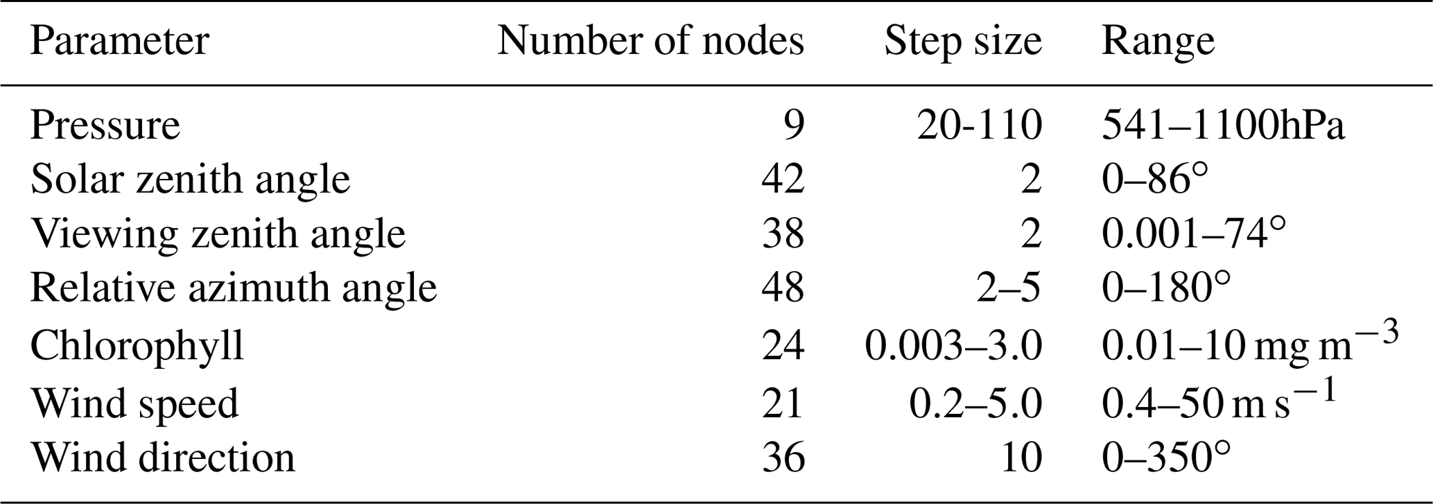
Appendix C: Description of lookup tables

Processing of GLER using online radiative transfer calculations is not efficient for the OMI mission due to their computationally expensive nature. Instead, LUT interpolation is used for the OMI mission, which speeds up the calculations significantly. To calculate GLER, two separate LUTs were generated: one for the TOA radiances calculated to include geometry-dependent surface BRDF effects and the other to derive LER from these radiances using the quantities I_o, S_b, and T, as described in Sect. 2.5. I_o, S_b, and T depend only on viewing geometries and surface pressure, whereas the TOA radiance table additionally included dependencies on chlorophyll, wind speed, and wind direction. The LUT nodes for the TOA radiance table shown in Table C1 were chosen by analyzing TOA radiance as a function of each input parameter to keep the interpolation error below 0.5 %.

Table C1LUT structure for TOA radiance calculations.

Download Print Version | Download XLSX

Author contributions

ZF led the paper and evaluation efforts. ZF, DH, AV, and RS wrote the paper. ZF and DH designed the GLER analysis. WQ carried out aerosol implementation and VLIDORT-related simulations. NK and JJ provided guidance throughout the development of the manuscript. All authors contributed to the editing of the manuscript. RS and AMS developed the VLIDORT code used for the BRDF and radiance computations.

Competing interests

The authors declare that they have no conflict of interest.

Acknowledgements

Funding for this work was provided by NASA through Aura core team funding, the Aura project, the Aura Science Team, and the Atmospheric Composition Modeling and Analysis Program, managed by Kenneth Jucks and Barry Lefer. We thank Patricia Castellanos and GMAO for providing us with the assimilated aerosol dataset. We thank David Antoine for useful discussions and for providing data on the bidirectional aspects of water-leaving radiance. Additionally, we thank the MODIS and OMI teams for providing the calibrated datasets.

Financial support

This research has been supported by the Atmospheric Composition Modeling and Analysis Program (grant no. NNH16ZDA001N-ACMAP).

Review statement

This paper was edited by Jun Wang and reviewed by two anonymous referees.

References

Ahn, C., Torres, O., and Jethva, H.: Assessment of OMI near-UV aerosol optical depth over land, J. Geophys. Res.-Atmos., 119, 2457–2473, https://doi.org/10.1002/2013JD020188, 2014. a

Austin, R. W.: The remote sensing of spectral radiance from below the ocean surface, Optical Aspects of Oceanography, edited by: Jerlov, N. G. and Nielsen, E. S., Academic Press, London, 317–344, 1974. a

Cetinic, I., McClain, C. R., and Werdell, P. J.: Pre-Aerosol, Clouds, and Ocean Ecosystem (PACE) Mission Science Definition Team Report, Volume 2, PACE Technical Report Series, 2018. a

Cox, C. and Munk, W.: Statistics of the sea surface derived from sun glitter, J. Mar. Res., 13, 198–227, 1954. a, b, c

Dave, J. V.: Effect of aerosol on the estimation of total ozone in an atmospheric column from the measurements of the ultraviolet radiance, J. Atmos. Sci., 35, 899–911, https://doi.org/10.1175/1520-0469(1978)035<0899:EOAOTE>2.0.CO;2, 1978. a

Dobber, M., Kleipool, Q., Dirksen, R., Levelt, P., Jaross, G., Taylor, S., Kelly, T., Flynn, L., Leppelmeier, G., and Rozemeijer, N.: Validation of Ozone Monitoring Instrument level 1b data products, J. Geophys. Res, 113, D15S06, https://doi.org/10.1029/2007JD008665, 2008. a, b, c

Frouin, R., Schwindling, M., and Deschamps, P.Y.: Spectral reflectance of sea foam in the visible and near infrared: In situ measurements and remote sensing implications, J. Geophys. Res., 101, 14361–14371, 1996. a

Gelaro, R., McCarty, W., Suárez, M.J., Todling, R., Molod, A., Takacs, L., Randles, C.A., Darmenov, A., Bosilovich, M.G., Reichle, R., Wargan, K., Coy, L., Cullather, R., Draper, C., Akella, S., Buchard, V., Conaty, A., da Silva, A.M., Gu, W., Kim, G., Koster, R., Lucchesi, R., Merkova, D., Nielsen, J.E., Partyka, G., Pawson, S., Putman, W., Rienecker, M., Schubert, S.D., Sienkiewicz, M., and Zhao, B.: The Modern-Era Retrospective Analysis for Research and Applications, Version 2 (MERRA-2), J. Climate, 30, 5419–5454, https://doi.org/10.1175/JCLI-D-16-0758.1, 2017. a

Gordon, H. R.: Can the Lambert-Beer law be applied to the diffuse attenuation coefficient of ocean water?, Limnol. Oceanogr., 34, 1389–1409, https://doi.org/10.4319/lo.1989.34.8.1389, 1989. a

Gordon, H. R. and Wang M.: Retrieval of water-leaving radiance and aerosol optical thickness over the oceans with SeaWiFS: A preliminary algorithm, Appl. Opt., 33, 443–452, https://doi.org/10.1364/AO.33.000443, 1994. a

Hale, G. M. and Querry, M.R..: Optical constants of water in the 200 nm to 200 µ wavelength region, Appl. Opt., 12, 555–563, https://doi.org/10.1364/AO.12.000555, 1973. a

Hu, C., Lee, Z., and Franz, B.: Chlorophyll-a algorithms for oligotrophic oceans: A novel approach based on three-band reflectance difference, J. Geophys. Res., 117, C01011, https://doi.org/10.1029/2011JC007395, 2012. a

Imaoka, K., Maeda, T., Kachi, M., Kasahra, M., Ito, N., and Nakagawa, K.: Status of AMSR2 instrument on GCOM-W1, Proc. SPIE, 8528, 852815, https://doi.org/10.1117/12.977774, 2012. a

Jaross, G. and Warner, J.: Use of Antarctica for validating reflected solar radiation measured by satellite sensors, J. Geophys. Res., 113, D16S34, https://doi.org/10.1029/2007JD008835, 2008. a

Joiner, J.: OMI/Aura and MODIS/Aqua Merged Cloud Product 1-Orbit L2 Swath 13 × 24 km V003, Greenbelt, MD, USA, Goddard Earth Sciences Data and Information Services Center (GES DISC), available at: https://disc.gsfc.nasa.gov/datacollection/OMMYDCLD_003.html (last access: 3 June 2019), 2014. a

Kaufman, Y., Remer, L., Tanre, D., Li, R., Kleidman, R., Mattoo, S., Levy, R., Eck, T., Holben, B., Ichoku, C., Martins, J., and Koren, I.: A critical examination of the residual cloud contamination and diurnal sampling effects on MODIS estimates of aerosol over ocean, IEEE T. Geosci. Remote, 43, 2886–2897, https://doi.org/10.1109/TGRS.2005.858430, 2005. a

Kay, S., Hedley, J.D., and Lavender, S.: Sun glint correction of high and low spatial resolution images of aquatic scenes: a review of methods for visible and near-Infrared wavelengths, Remote Sens., 1, 697–730, https://doi.org/10.3390/rs1040697, 2009. a

Kleipool, Q. L., Dobber, M. R., de Haan, J. F., and Levelt, P. F.: Earth surface reflectance climatology from 3 years of OMI data, J. Geophys. Res., 113, D18308, https://doi.org/10.1029/2008jd010290, 2008. a, b

Koelemeijer, R. B. A., Stammes, P., Hovenier, J. W., and de Haan, J. F.: A fast method for retrieval of cloud parameters using oxygen A-band measurements from the Global Ozone Monitoring Experiment, J. Geophys. Res., 106, 3475–3496, https://doi.org/10.1029/2000JD900657, 2001. a

Koelemeijer, R. B. A., de Haan, J. F., and Stammes, P.: A database of spectral surface reflectivity in the range 335–772 nm derived from 5.5 years of GOME observations, J. Geophys. Res., 108, 4070, https://doi.org/10.1029/2002JD002429, 2003. a

Krotkov, N. A., Lamsal, L. N., Celarier, E. A., Swartz, W. H., Marchenko, S. V., Bucsela, E. J., Chan, K. L., Wenig, M., and Zara, M.: The version 3 OMI NO2 standard product, Atmos. Meas. Tech., 10, 3133–3149, https://doi.org/10.5194/amt-10-3133-2017, 2017. a

Lamsal, L. N., Krotkov, N. A., Celarier, E. A., Swartz, W. H., Pickering, K. E., Bucsela, E. J., Gleason, J. F., Martin, R. V., Philip, S., Irie, H., Cede, A., Herman, J., Weinheimer, A., Szykman, J. J., and Knepp, T. N.: Evaluation of OMI operational standard NO₂ column retrievals using in situ and surface-based NO2 observations, Atmos. Chem. Phys., 14, 11587–11609, https://doi.org/10.5194/acp-14-11587-2014, 2014. a

Lee, Z. and Hu, C.: Global distribution of Case-1 waters: An analysis from SeaWiFS measurements, Remote Sens. Environ., 101, 270–276, https://doi.org/10.1016/j.rse.2005.11.008, 2006. a

Lee, Z., Hu, C., Shang, S., Du, K., Lewis, M., Arnone, R., and Brewin, R.: Penetration of UV-visible solar radiation in the global oceans: Insights from ocean color remote sensing, J. Geophys. Res.-Oceans, 118, 4241–4255, https://doi.org/10.1002/jgrc.20308, 2013. a

Lee, Z., Wei, J., Voss, K., Lewis, M., Bricaud, A., and Huot, Y.: Hyperspectral absorption coefficient of “pure” seawater in the range of 350–550 nm inverted from remote sensing reflectance, Appl. Opt., 54, 546–558, https://doi.org/10.1364/AO.54.000546, 2015. a, b, c

Lee, Z. P., Du, K. P., and Arnone, R.: A model for the diffuse attenuation coefficient of downwelling irradiance, J. Geophys. Res., 110, C02016, https://doi.org/10.1029/2004JC002275, 2005. a, b

Levelt, P. F., Joiner, J., Tamminen, J., Veefkind, J. P., Bhartia, P. K., Stein Zweers, D. C., Duncan, B. N., Streets, D. G., Eskes, H., van der A, R., McLinden, C., Fioletov, V., Carn, S., de Laat, J., DeLand, M., Marchenko, S., McPeters, R., Ziemke, J., Fu, D., Liu, X., Pickering, K., Apituley, A., González Abad, G., Arola, A., Boersma, F., Chan Miller, C., Chance, K., de Graaf, M., Hakkarainen, J., Hassinen, S., Ialongo, I., Kleipool, Q., Krotkov, N., Li, C., Lamsal, L., Newman, P., Nowlan, C., Suleiman, R., Tilstra, L. G., Torres, O., Wang, H., and Wargan, K.: The Ozone Monitoring Instrument: overview of 14 years in space, Atmos. Chem. Phys., 18, 5699–5745, https://doi.org/10.5194/acp-18-5699-2018, 2018. a

Lucchesi, R.: File Specification for GEOS-5 FP-IT, GMAO Office Note No. 2 (Version 1.2), 60 pp., available at: http://gmao.gsfc.nasa.gov/pubs/office_notes (1 June 2019), 2013. a

Menzel, W., Frey, R., Zhang, H., Wylie, D., Moeller, C., Holz, R., Maddux, B., Baum, B., Strabala, K., and Gumley, L.: MODIS global cloud-top pressure and amount estimation: algorithm description and results. J. Appl. Meteorol. Climatolol., 47, 1175–1198, https://doi.org/10.1175/2007JAMC1705.1, 2007. a

Mishchenko, M. I. and Travis, L. D.: Satellite retrieval of aerosol properties over the ocean using polarization as well as intensity of reflected sunlight, J. Geophys. Res., 102, 16989–17013, https://doi.org/10.1029/96JD02425, 1997. a

Moore, T. S., Campbell, J. W., and Dowell, M. D.: A class-based approach to characterizing and mapping the uncertainty of the MODIS ocean chlorophyll product, Remote Sens. Environ., 113, 2424–2430, https://doi.org/10.1016/j.rse.2009.07.016, 2009. a

Morel, A.: Optical modeling of the upper ocean in relation to its biogeneous matter content (Case I waters), J. Geophys. Res., 93, 10749–10768, https://doi.org/10.1029/JC093iC09p10749, 1988. a, b

Morel, A. and Gentili, B.: Diffuse reflectance of oceanic waters : its dependence on sun angles as influenced by molecular scattering contribution, Appl. Optics, 30, 4427–4438, https://doi.org/10.1364/AO.30.004427, 1991. a

Morel, A. and Gentili, B.: Bidirectional reflectance of oceanic waters: accounting for Raman emission and varying particle scattering phase function, Appl. Optics, 41, 6289–6306, https://doi.org/10.1364/AO.41.006289, 1992. a

Morel, A. and Gentili, B.: Diffuse reflectance of oceanic waters (2): bidirectional aspects, Appl. Optics, 32, 6864–6879, https://doi.org/10.1364/AO.32.006864, 1993. a

Morel, A. and Gentili, B.: Diffuse reflectance of oceanic water. III. Implication of bidirectionality for the remote-sensing probe, Appl. Optics, 35, 4850–4862, https://doi.org/10.1364/AO.35.004850, 1996. a, b, c

Morel, A. and Maritorena, S.: Bio-optical properties of oceanic waters: A reappraisal, J. Geophys Res., 106, 7163–7180, https://doi.org/10.1029/2000JC000319, 2001. a, b, c, d, e, f

Morel, A., Antoine, D., and Gentili, B.: Bidirectional reflectance of oceanic waters: Accounting for Raman emission and varying particle scattering phase function, Appl. Opt., 41, 6289–6306, https://doi.org/10.1364/AO.41.006289, 2002. a, b

Morel, A., Gentili, B., Claustre, H., Bricaud, A., Ras, J., and Tiche, F.: Optical properties of the clearest natural waters, Limnol. Oceanogr., 20, 177–184, https://doi.org/10.4319/lo.2007.52.1.0217, 2007. a, b

Nazaryan, H., McCormick, M. P., and Menzel, W. P.: Global characterization of cirrus clouds using CALIPSO data, J. Geophys. Res., 113, D16211, https://doi.org/10.1029/2007JD009481, 2008. a

Park, Y. and Rudick, M.: Model of remote-sensing reflectance including bidirectional effects for case 1 and case 2 waters, Appl. Opt., 44, 1236–1249, https://doi.org/10.1364/AO.44.001236, 2005. a

Pope, R. M. and Fry, E. S.: Absorption spectrum (380–700 nm) of pure water, II, Integrating cavity measurements, Appl. Opt., 36, 8710–8723, https://doi.org/10.1364/AO.36.008710, 1997. a

Qin, W., Fasnacht, Z., Haffner, D., Vasilkov, A., Joiner, J., Krotkov, N., Fisher, B., and Spurr, R.: A geometry-dependent surface Lambertian-equivalent reflectivity product for UV–Vis retrievals – Part 1: Evaluation over land surfaces using measurements from OMI at 466 nm, Atmos. Meas. Tech., 12, 3997–4017, https://doi.org/10.5194/amt-12-3997-2019, 2019. a, b, c

Quickenden, T. I. and Irvin, J. A.: The ultraviolet absorption spectrum of liquid water, J. Chem. Phys., 72, 4416–4428, https://doi.org/10.1063/1.439733, 1980. a

Randles, C. A., Silva, A. M. D., Buchard, V., Colarco, P. R., Darmenov, A., Govindaraju, R., Smirnov, A., Holben, B., Ferrare, R., Hair, J., Shinozuka, Y., and Flynn, C. J.: The MERRA-2 aerosol reanalysis, 1980 onward, Part I: system description and data assimilation evaluation, J. Climate, 30, 6823–6850, https://doi.org/10.1175/JCLI-D-16-0609.1, 2017. a, b

Sayer, A. M., Thomas, G. E., and Grainger, R. G.: A sea surface reflectance model for (A)ATSR, and application to aerosol retrievals, Atmos. Meas. Tech., 3, 813–838, https://doi.org/10.5194/amt-3-813-2010, 2010. a

Sayer, A. M., Hsu, N. C., Bettenhausen, C., Holz, R. E., Lee, J., Quinn, G., and Veglio, P.: Cross-calibration of S-NPP VIIRS moderate-resolution reflective solar bands against MODIS Aqua over dark water scenes, Atmos. Meas. Tech., 10, 1425–1444, https://doi.org/10.5194/amt-10-1425-2017, 2017. a, b

Schaepman-Strub, G., Schaepman, M. E., Painter, T. H., Dangel, S., and Martonchik, J. V.: Reflectance quantities in optical remote sensing: definitions and case studies, Remote Sens. Environ., 103, 27–42, https://doi.org/10.1016/j.rse.2006.03.002, 2006. a

Schenkeveld, V. M. E., Jaross, G., Marchenko, S., Haffner, D., Kleipool, Q. L., Rozemeijer, N. C., Veefkind, J. P., and Levelt, P. F.: In-flight performance of the Ozone Monitoring Instrument, Atmos. Meas. Tech., 10, 1957–1986, https://doi.org/10.5194/amt-10-1957-2017, 2017. a, b, c, d

Seftor, C. J., Taylor, S. L., Wellemeyer, C. G., and McPeters, R. D.: Effect of Partially-Clouded Scenes on the Determination of Ozone, in: Ozone in the Troposphere and Stratosphere, Part 1, Proceedings of the Quadrennial Ozone Symposium, Charlottesville, USA, 1992, NASA Conference Publication 3266, 919–922, 1994. a

Spurr, R. J. D.: VLIDORT: a linearized pseudo-spherical vector discrete ordinate radiative transfer code for forward model and retrieval studies in multilayer multiple scattering media, J. Quant. Spectrosc. Ra., 102, 316–421, https://doi.org/10.1016/j.jqsrt.2006.05.005, 2006. a

Spurr, R. and Christi, M.: The LIDORT and VLIDORT Linearized Scalar and Vector Discrete Ordinate Radiative Transfer Models: Updates in the last 10 Years. Light Scattering Reviews, Volume 12, edited by: Kokhanovsky, A., Springer, Cham, Switzerland, 2019. a, b

Spurr, R., Stamnes, K., Eide, H., Li, W., Zhang, K., and Stamnes, J.: Simultaneous Retrieval of Aerosols and ocean properties: A classic inverse modeling approach, I, Analytic jacobians from the Linearized CAO-DISORT model, J. Quant. Spectrosc. Ra., 104, 428–449, https://doi.org/10.1016/j.jqsrt.2006.09.009, 2007. a

Stammes, P., Sneep, M., de Haan, J. F., Veefkind, J. P., Wang, P., and Levelt, P. F.: Effective cloud fractions from the Ozone Monitoring Instrument: Theoretical framework and validation, J. Geophys. Res., 113, D16S38, https://doi.org/10.1029/2007JD008820, 2008. a

Szeto, M., Werdell, P. J., Moore, T. S., and Campbell, J. W.: Are the world's oceans optically different?, J. Geophys. Res., 116, C00H04, https://doi.org/10.1029/2011JC007230, 2011. a

Thomas , G. and Stamnes, K.: Radiative transfer in the atmosphere and ocean, Cambridge University Press, New York, NY, 1999. a

Tilstra, L. G., Tuinder, O. N. E., Wang, P., and Stammes, P.: Surface reflectivity climatologies from UV to NIR determined from Earth observations by GOME-2 and SCIAMACHY, J. Geophys. Res., 122, 4084–4111, https://doi.org/10.1002/2016JD025940, 2017. a

Torres, O., Bhartia, P., Herman, J., Ahmad, Z., and Gleason, J.: Derivation of aerosol properties from satellite measurments of backscattered ultraviolet ratiadtion: Theoretical basis, J. Geophys. Res., 110, D14, https://doi.org/10.1029/98JD00900, 1998. a

Torres, O., Tanskanen, A., Veihelman, B., Ahn, C., Braak, R., Bhartia, P. K., Veefkind, V., and Levelt, P.: Aerosols and surface UV products from OMI observations: an overview, J. Geophys. Res., 112, D24S47, https://doi.org/10.1029/2007JD008809, 2007. a, b

Vasilkov, A., Joiner, J., Bhartia, P., Levelt, P., and Stephens, G.: Evaluation of the OMI cloud pressured derived from the rotational Raman scattering by comparisons with other satellite data and radiative transfer simulations, J. Geophys., Res., 113, D15S19, https://doi.org/10.1029/2007JD008689, 2008. a, b

Vasilkov, A., Qin, W., Krotkov, N., Lamsal, L., Spurr, R., Haffner, D., Joiner, J., Yang, E.-S., and Marchenko, S.: Accounting for the effects of surface BRDF on satellite cloud and trace-gas retrievals: a new approach based on geometry-dependent Lambertian equivalent reflectivity applied to OMI algorithms, Atmos. Meas. Tech., 10, 333–349, https://doi.org/10.5194/amt-10-333-2017, 2017. a, b, c, d

Vasilkov, A., Yang, E.-S., Marchenko, S., Qin, W., Lamsal, L., Joiner, J., Krotkov, N., Haffner, D., Bhartia, P. K., and Spurr, R.: A cloud algorithm based on the O₂-O₂ 477 nm absorption band featuring an advanced spectral fitting method and the use of surface geometry-dependent Lambertian-equivalent reflectivity, Atmos. Meas. Tech., 11, 4093–4107, https://doi.org/10.5194/amt-11-4093-2018, 2018. a

Vasilkov, A. P., Herman, J., Krotkov, N. A., Kahru, M., Mitchell, B. G., and Hsu, C.: Problems in assessment of the UV penetration into natural waters from space-based measurements, Opt. Eng., 41, 3019–3027, https://doi.org/10.1117/1.1516822, 2002. a, b

Vasilkov, A. P., Herman, J. R., Ahmad, Z., Karu, M., and Mitchell, B. G.: Assessment of the ultraviolet radiation field in ocean waters from space-based measurements and full radiative-transfer calculations, Appl. Opt., 44, 2863–2869, https://doi.org/10.1364/AO.44.002863, 2005. a, b, c

Veefkind, J. P., de Haan, J. F., Sneep, M., and Levelt, P. F.: Improvements to the OMI O₂–O₂ operational cloud algorithm and comparisons with ground-based radar–lidar observations, Atmos. Meas. Tech., 9, 6035–6049, https://doi.org/10.5194/amt-9-6035-2016, 2016. a

Wentz, F. J. and Meissner, T.: AMSR Ocean Algorithm Theoretical Basis Document, Version 2, Remote Sensing Systems, Santa Rosa, CA, 2000. a

Wentz, F. J. and Meissner, T.: AMSR-E/Aqua L2B Global Swath Ocean Products Derived from Wentz Algorithm V002 (January 2009, June to August 2010). Updated daily, Boulder, Colorado USA: National Snow and Ice Data Center, Digital media, 2004. a

Wentz, F. and Meissner, T.: Supplement 1: Algorithm theoretical basis document for AMSR-E ocean algorithms, Santa Rosa, CA: Remote Sensing Systems, 2007. a

Wentz, F., Hilburn, K., and Smith, K.: RSS SSMIS ocean product grids daily from DMSP F16 NETCDF. Dataset available online from the NASA Global Hydrology Resource Center DAAC, Huntsville, Alabama, USA, https://doi.org/10.5067/MEASURES/DMSP-F16/SSMIS/DATA301, 2012. a

Werdell, P. J., Behrenfeld, M. J., Bontempi, P. S., Boss, E., Cairns, B., Davis, G. T., Franz, B. A., Gliese, U. B., Gorman, E. T., Hasekamp, O., Knobelspiesse, K. D., Mannino, A., Martins, J. V., McClain, C. R., Meister, G., and Remer, L. A.: The Plankton, Aerosol, Cloud, Ocean Ecosystem Mission: Status, Science, Advances, B. Am. Meteorol. Soc., 100, 1775–1794, https://doi.org/10.1175/BAMS-D-18-0056.1, 2019. a

Westberry, T. K., Boss, E., and Lee, Z.: Influence of Raman scattering on ocean color inversion models, Appl. Opt., 52, 5552–5561, https://doi.org/10.1364/AO.52.005552, 2013. a

Articles

Short summary

The anisotropy of Earth's surface reflection plays an important role in satellite-based retrievals of cloud, aerosol, and trace gases. Most current ultraviolet and visible satellite retrievals utilize climatological surface reflectivity databases that do not account for surface anisotropy. The GLER concept was introduced to account for such features. Here we evaluate GLER for water surfaces by comparing with OMI measurements and show that it captures these surface anisotropy features.