the Creative Commons Attribution 4.0 License.
the Creative Commons Attribution 4.0 License.
 | 06 Feb 2019
Joint retrieval of surface reflectance and aerosol properties with continuous variation of the state variables in the solution space – Part 2: application to geostationary and polar-orbiting satellite observations
Marta Luffarelli
Yves Govaerts
This paper presents the simultaneous retrieval of aerosol optical thickness and surface properties from the CISAR algorithm applied both to geostationary and polar-orbiting satellite observations. The theoretical concepts of the CISAR algorithm have been described in Govaerts and Luffarelli (2018). CISAR has been applied to SEVIRI and PROBA-V observations acquired over 20 AERONET stations during the year 2015. The CISAR retrieval from the two sets of observations is evaluated against independent data sets such as the MODIS land product and AERONET data. The performance differences resulting from the two types of orbit are discussed, and the information content of SEVIRI and PROBA-V observations is analysed and compared.
- Article
(4981 KB) - Companion paper
-
Supplement
(648 KB) - BibTeX
- EndNote


The retrieval of aerosol properties over land surfaces from space observations is a challenging problem due to the strong radiative coupling between atmospheric and surface radiative processes. Different approaches are usually exploited to retrieve different Earth system components (e.g. Hsu et al., 2013, Mei et al., 2017), leading to inconsistent and less accurate data sets. The joint retrieval of surface reflectance and aerosol properties, as originally proposed by Pinty et al. (2000), presents many advantages, such as the possibility to perform the retrieval over any type of surface and ensure radiative consistency among the retrieved variables.
Govaerts and Luffarelli (2018) (hereafter referred to as Part 1) describes the theoretical aspects of the Combined Inversion of Surface and AeRosol (CISAR) algorithm, designed for the joint retrieval of surface reflectance and aerosol properties. This new generic retrieval method specifically addresses issues related to the continuous variation of the state variables in the solution space within an optimal estimation (OE) framework. Through a set of experiments, the capability of CISAR to retrieve surface reflectance and aerosol properties within the solution space was illustrated. Nonetheless, these experiments only represent ideal simulated observation conditions, i.e. noise-free data acquired in narrow spectral bands placed in the principal plane, assuming unbiased surface prior information. This second part aims to demonstrate CISAR's applicability to actual satellite observations, with less favourable geometrical conditions than the principal plane and accounting for the radiometric noise. For this purpose, the algorithm has been applied to two radiometers with similar spectral properties but different orbits (geostationary and polar). Radiometers on board geostationary platforms deliver observations with a revisit time of tens of minutes but with a limited field of view, so that many instruments are needed to cover the entire Earth. The poles cannot be observed. Conversely, a polar orbit, combined with an adequate swath, could offer a daily revisit time of the entire globe. The selected radiometers are the Spinning Enhanced Visible and Infrared Imager (SEVIRI), flying on board of the Meteosat Second Generation (MSG) geostationary platform, and the PRoject for On-Board Autonomy-Vegetation (PROBA-V). These two instruments have similar radiometric performances and both have acquired more than 15 years of observations thanks to the launch of a succession of radiometers with very similar characteristics. Applying the same algorithm on similar instruments flying in different orbits represents a meaningful way to analyse the generic algorithm performance of CISAR.
This paper is organised as follows. Section 2 describes the observation system considered in the OE framework: the satellite observation, the ancillary information, the prior information and the forward model. The uncertainty characterisation of the observation system is also described in Sect. 2. The algorithm implementation is described in Sect. 3. Section 4 analyses the information content of the satellite observations, comparing the differences between the geostationary and polar-orbiting instruments, and discusses the challenges encountered when little or no information about the retrieved variables is carried by the observation. Given these difficulties in the retrieval, a quality indicator (QI) is implemented and presented in Sect. 5, characterising the reliability of the solution. Finally, the performance of CISAR is discussed in detail in Sect. 6. The derivation of CISAR-retrieved aerosol optical thickness (AOT) and bidirectional hemispherical reflectance (BHR) will be compared between the AErosol RObotic NETwork (AERONET) (Giles et al., 2017) and the Moderate Resolution Imaging Spectroradiometer (MODIS) land product data (DAAC, 2017). The performance differences between the retrieved data sets obtained from SEVIRI and PROBA-V observations will be further investigated through statistics on the quality of the retrieval and through the information content of the satellite observations.
2.1 Observation system definition
The fundamental principle of OE is to maximise the probability with respect to the values of the state vector x, conditional to the value of the measurements and any prior information (Rodgers, 2000). The ensemble of measurements, prior information, ancillary data and the forward model constitutes the observation system. This section describes each component of this system for the two satellite data sets processed in the framework of this study.
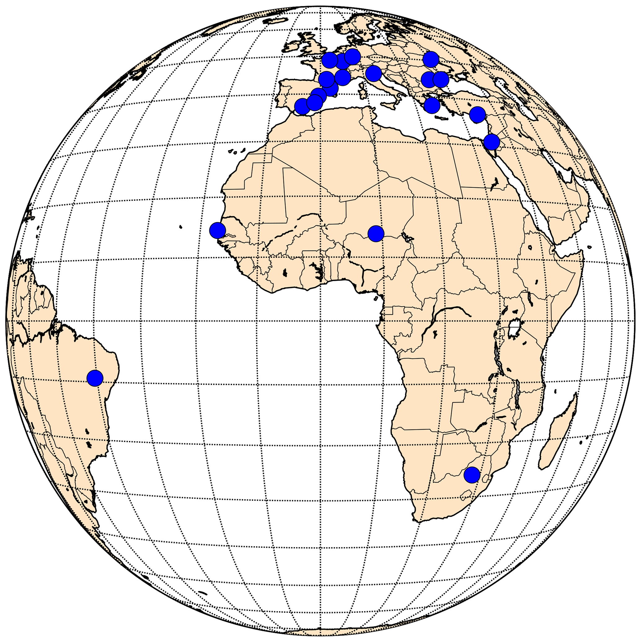
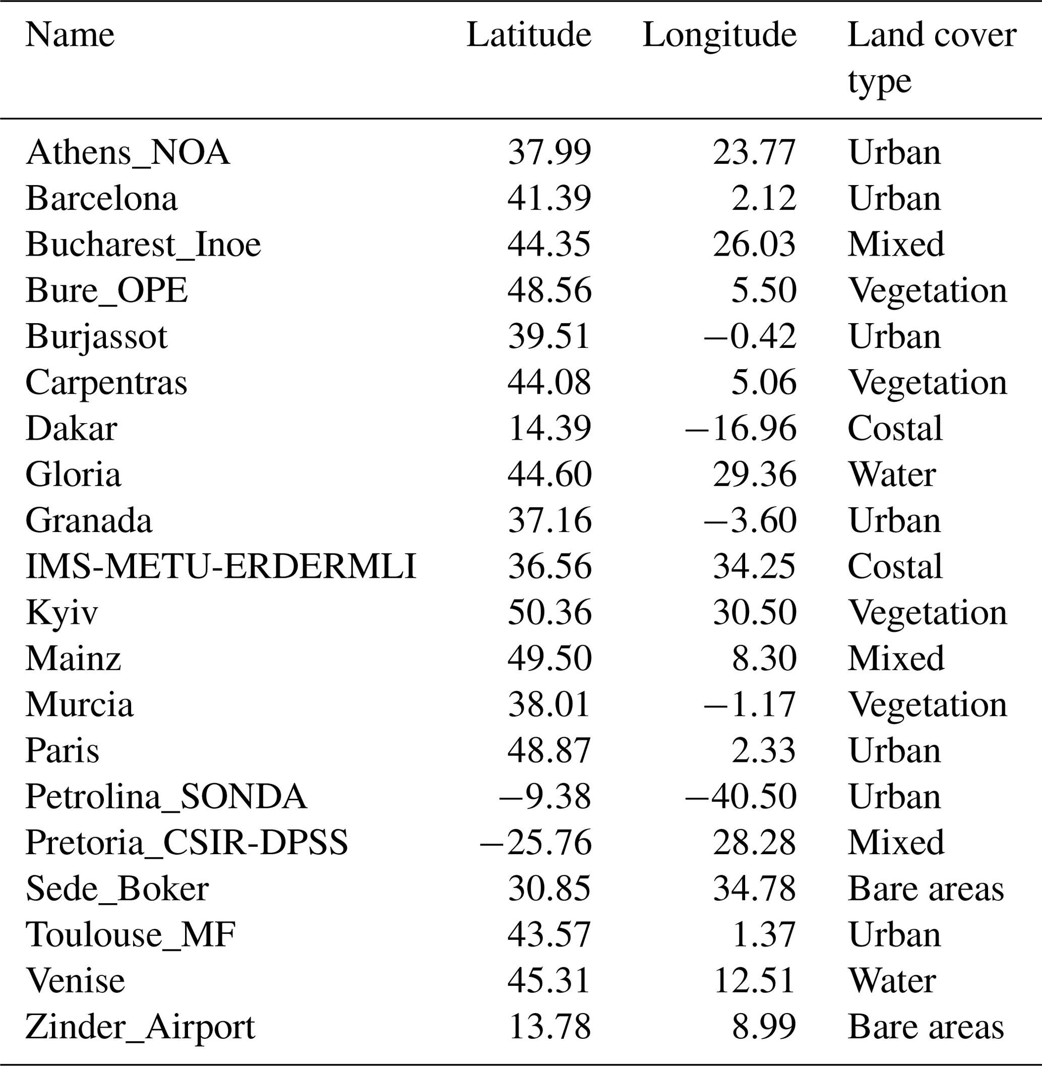
Figure 1Locations of selected AERONET stations. All stations are located within the SEVIRI field of view.
In order to evaluate the CISAR algorithm performance when applied to observations acquired from different orbits, 20 AERONET stations located within the SEVIRI field of view have been selected (Fig. 1, Table 1). These targets span different geometries and land cover types (vegetation, urban, bare areas, water, mixed). The observations pertain to the year 2015.
For each of these stations, satellite data have been acquired, together with ancillary information, such as the cloud mask and the model parameters, which are the parameters that are not retrieved by the algorithm but that influence the observation. Satellite data and ancillary information are accumulated in time to form a multi-angular observation vector in order to correctly characterise the surface reflectance anisotropy. Nevertheless, retrieving surface and aerosol properties from satellite observations is an ill-posed problem (Wang, 2012). Consequently, assumptions on the magnitude and on the temporal and spectral variability of the state variables are made. The ensemble of these assumptions and their associated uncertainties constitutes the prior information.
The observation uncertainty sigmao characterisation is one of the most critical aspects of the CISAR algorithm as it directly determines the likelihood of the solution. In fact, sigmao determines the observation term of the cost function (Eq. 17 of Part 1). The observation uncertainty is composed of the radiometric uncertainty (directly related to the radiometer characteristics), the forward model uncertainty and the uncertainty related to the model parameters.
2.2 Satellite data
MSG nominal position is 0∘ over the equator in a geostationary orbit. SEVIRI is the main instrument of the MSG mission, which has as its primary objective the observation in near real-time of the Earth's full disk, shown in Fig. 1. SEVIRI achieves this with 12 channels, ranging from 0.6 to 13 µm, three of which are located in the solar spectrum and centred at 0.64, 0.81 and 1.64 µm and are used within this study. SEVIRI observes the Earth's full disk with a 15 min repeat cycle. The sampling distance between two adjacent pixels at the subsatellite point is 3 km for the visible bands. As there is no on-board device for the calibration of the solar channels, the calibration within this study has been performed with the method proposed by Govaerts et al. (2013).
The PROBA-V satellite mission is intended to ensure the continuation of the Satellite Pour l'Observation de la Terre 5 (SPOT5) VEGETATION products starting from May 2014 (Sterckx et al., 2014). The microsatellite offers global coverage of land surface with daily revisit for latitude from 75∘ N to 56∘ S in four spectral bands, centred at 0.46, 0.66, 0.83 and 1.61 µm. The PROBA-V products are provided at a spatial resolution of 1∕3 and 1 km, the latter being used in the framework of this study. To cover the wide angular field of view (101∘) in a small-sized platform, the optical design of PROBA-V is made up of three cameras (identical three-mirror anastigmatic telescopes). The three cameras have an equal field of view. The downward-pointing central camera covers a swath 500 km wide, while the swath of the right and left cameras is 875 km wide. Although the three cameras have different responses, a mean spectral response function (SRF) is considered within this study, accounting for the radiometric uncertainty associated with this approximation. Each camera has two focal planes, one for the short-wave infrared (SWIR) band and one for the visible and near-infrared (VNIR) bands. Despite the different viewing angles in the SWIR band, CISAR assumes the observations are acquired with the same geometry in all bands. This assumption leads to an additional term in the observation uncertainty. Because of the omission of on-board calibration devices, the PROBA-V in-flight calibration relies only on vicarious methods (Sterckx et al., 2013).
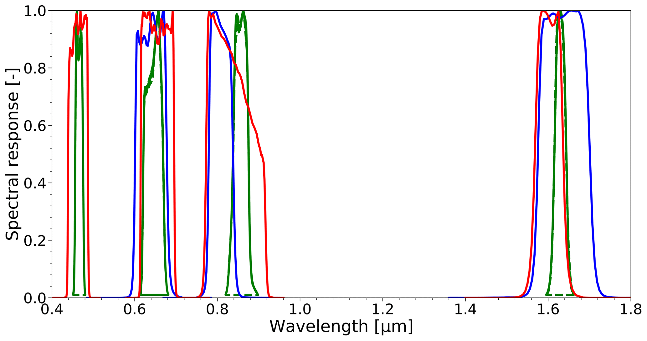
The similarities between the three SEVIRI solar bands and the red, NIR and SWIR PROBA-V bands permit the evaluation and comparison of the CISAR performances when applied to the two instruments, the spectral responses of which are shown in Fig. 2. The satellite observations have been acquired from the European Organisation for the Exploitation of Meteorological Satellites (EUMETSAT) Earth Observation Portal and from the Flemish Institute for Technological Research (VITO) for SEVIRI and PROBA-V respectively. The top-of-atmosphere (TOA) bidirectional reflectance factor (BRF) satellite observation uncertainty is derived is computed directly from the digital count value in the case of SEVIRI, whereas for PROBA-V the level 2-A TOA BRF is provided by VITO (Wolters et al., 2018). The satellite observation uncertainty is derived from the radiometric noise σi and the geolocation uncertainty σr. For PROBA-V two additional terms are calculated: the uncertainty σc associated with the approximation of a mean SRF of the cameras and the one derived from considering the same viewing geometry in the SWIR and in the VNIR bands, σΩ.
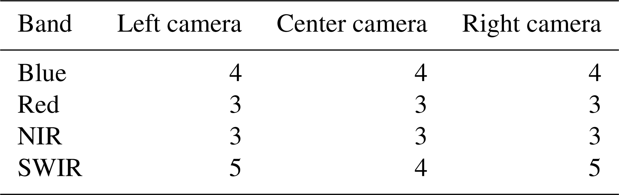
PROBA-V radiometric noise has been delivered by VITO (Sindy Sterckx, personal communication, September 2017) per camera and per band (Table 2). For SEVIRI, this term is computed considering (i) the instrument noise due to the dark current, (ii) the difference between the detector gain and (iii) the number of digitalisation levels (Govaerts and Lattanzio, 2007). The geolocation uncertainty σr, arising from the assumption of the satellite data being correctly mapped to the surface of the Earth, is estimated for each pixel p as follows (Govaerts et al., 2010):
where σx,y is the geolocation or co-registration standard deviation and is the TOA BRF in the channel acquired at time t.
The uncertainty σc, originating from the usage of a mean SRF for the three PROBA-V cameras, has been estimated by simulating the TOA BRF, considering both the mean and actual SRF for a wide range of observation conditions. The assessed σc is lower than 0.2 % in all bands and for all cameras. Finally, the assumption of having the same viewing geometry for the three PROBA-V bands is associated with the uncertainty σΩ, computed as follows:
The total relative radiometric uncertainty median values are shown in Table 3.
2.3 Ancillary data
In addition to satellite observations, a cloud mask and the model parameters are required. For SEVIRI observations, the nowcasting satellite application facility (SAF) cloud mask (Meteo France, 2013), provided at the radiometer's native temporal and spatial resolution, is used; for PROBA-V the cloud mask is provided by VITO (Wolters et al., 2018). The model parameters, i.e. total column water vapour (TCWV), total column ozone (TCO3) and surface pressure, are taken from the European Centre for Medium-Range Weather Forecasts (ECMWF) reanalysis (Dee et al., 2011).
The uncertainties of the model parameters b are converted into an equivalent noise σB, calculated as follows (Govaerts et al., 2010):
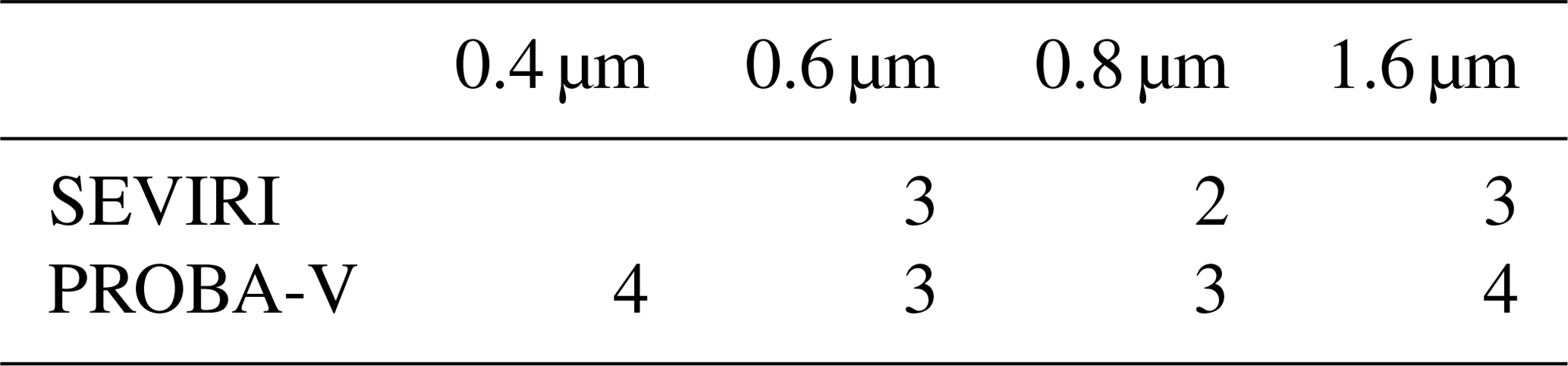
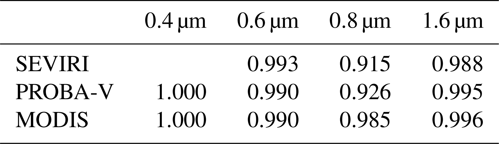
where Uoz and Uwv are the ozone and water vapour total column concentration, Usp is the surface pressure and , and are their associated uncertainties. The surface pressure contribution to the signal is about 10 times smaller than the contribution of the water vapour concentration. The TCWV is distributed among the two atmospheric layers in the forward radiative transfer model assuming a US76 water vapour vertical profile (Sissenwine et al., 1976). The fraction of TCWV in the scattering layer interacts with the aerosol particles and thus strongly affects the CISAR retrieval. Unlike the ozone which is mainly present in the stratosphere, the water vapour is dominant in the lower part of the atmosphere, severely impacting the aerosol retrieval in SEVIRI and PROBA-V band 0.8 µm (Table 4). Hence, only the uncertainty related to the TCWV is considered and Eq. (3) is approximated to the following:
Table 4Water vapour transmittance in the SEVIRI, PROBA-V and MODIS bands.
The median values of the equivalent model parameter noise (EQMPN), computed as in Eq. (4), are shown in Table 5.
2.4 Prior information
Within an OE framework, the definition of the prior information and its uncertainty plays a fundamental role. In CISAR four different sources of prior information are considered:
-
Surface parameter magnitude. The surface reflectance, represented by the RPV (Rahman–Pinty–Verstraete) model (Rahman et al., 1993), is not expected to undergo rapid variations on a short temporal scale; hence the retrieval in the previous accumulation period can be used as prior information for the next inversion (Govaerts et al., 2010). The prior information on the RPV parameters at the time td is built by computing a running mean over the Nr previously converged accumulation periods.
The corresponding prior uncertainty is defined as half of the variability range of the solution retrieved during the considered Nr accumulation periods.
When Nr is smaller than a certain minimum threshold Nmin (Table 7), the prior information on the magnitude of the RPV parameters is taken from the last successful retrieval and its uncertainty is computed as in Eq. (7), where Nd is the number of days since the last successful retrieval (Govaerts et al., 2017).
-
AOT magnitude. This information is taken from an annual mean climatology data set (Kinne et al., 2013). From this data set, the prior information on the AOT magnitude for the coarse and fine mode (absorbing and non-absorbing distinctly) is taken. The uncertainty is set to a high arbitrary value for all the wavelengths (Table 7).
-
Constraints on the AOT temporal variability. These constraints result from the assumption that the AOT does not change rapidly on a very short temporal scale; therefore a maximum temporal variation is defined through a sigmoid function. The temporal constraints are described by the matrix Ha in Eq. 13 of Part 1.
-
Constraints on the AOT spectral variability. The AOT is expected to decrease with the wavelength, proportionally to the ratio of the extinction coefficient (see Eq. 15 of Part 1). The applied constraints define the matrix Hl (Eq. 14 of Part 1).
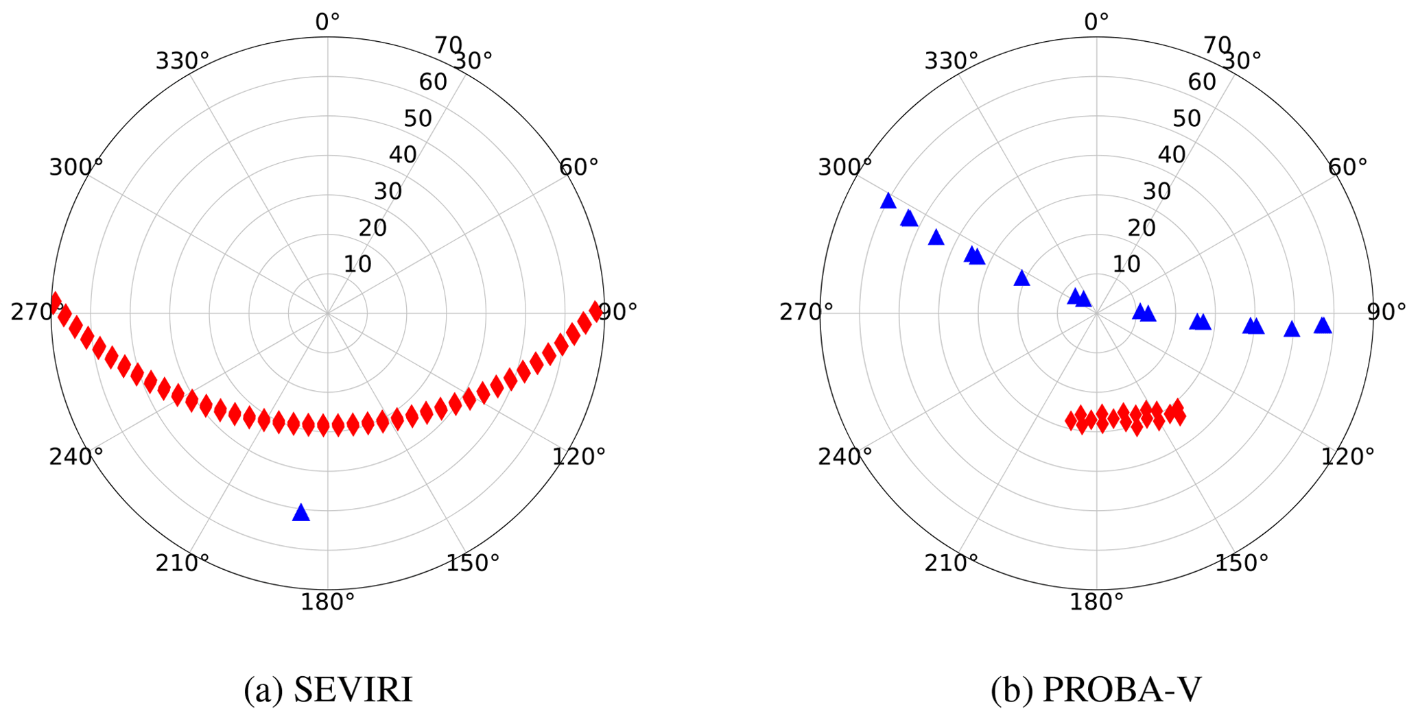
Figure 3Polar plot of the angular sampling during 5 days (1–5 May 2015) of SEVIRI observations (a) and during 16 days (1–16 May 2015) of PROBA-V observations (b) over Carpentras, France. The blue triangles represent the satellite viewing angles, the red diamonds the illumination one. Circles represent the zenith angle and polar angles represent azimuth angles with zero azimuth pointing to the North.
2.5 Forward model
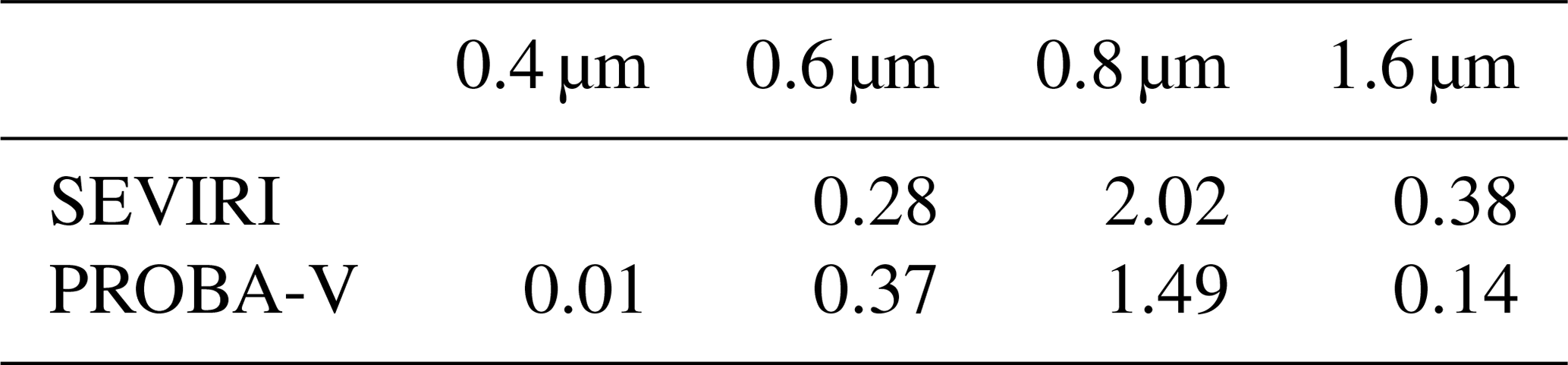
FASTRE, the CISAR forward radiative transfer model (RTM), and its uncertainty σF are described in Sect. 4.4 of Part 1. FASTRE uncertainty in the SEVIRI and PROBA-V processed bands has been estimated as in Eq. (10) of Part 1, comparing the outcome of FASTRE with a more elaborated RTM, in which 50 atmospheric layers are considered. The results of this evaluation are shown in Table 6. The forward model uncertainty is lower than 3 % in all processed bands, presenting its largest value in the SEVIRI VIS0.8 band, the most affected by water vapour absorption (Table 4). The FASTRE two-layer approximation of the atmosphere does not allow a correct discretisation of the water vapour vertical profile and, thus, a correct characterisation of its interaction with the scattering particles. Moreover, the two-layer approximation assumes that the scattering particles are only present in the lower layer. Given the spectral behaviour of the AOT, this assumption leads to a higher uncertainty at wavelengths shorter than 0.4 µm (Seidel et al., 2010). Despite the limitations associated with the two-layer approximation, FASTRE uncertainty is in the range of 1 %–3 % (Table 6), which is smaller or equal to the instrument radiometric noise.
Table 6FASTRE relative uncertainty in the SEVIRI and PROBA-V processed bands (%).

3.1 General set-up
In order to perform the inversion on actual satellite data, the observations are accumulated in time and the corresponding uncertainty is computed as described in Sect. 2. This temporal accumulation is performed in order to build a multi-angular observation vector to characterise the surface reflectance anisotropy. The surface optical properties are considered invariant during the accumulation period, and therefore a trade-off between having enough cloud-free observations to build the observation vector and allowing the algorithm to catch surface variations is introduced; the high-repeat temporal coverage of geostationary satellites allows a shorter accumulation periods with respect to polar-orbiting instruments. For SEVIRI acquisitions, although the angular sampling does not vary much from one day to the next, the length of the accumulation period is set to 5 days in order to maximise the occurrence of cloud-free observations. For polar-orbiting satellites, the length of the temporal accumulation is normally driven by the repeat cycle, as it is the case for MODIS (DAAC, 2018). In the case of PROBA-V, the satellite orbit is not maintained and there is no repeat cycle. Hence, the choice of the length of the time window during which the satellite observations are accumulated results from empirical studies, aiming to balance the trade-off previously described. Consequently, the length of the accumulation is set to 16 days and the successive accumulation periods are shifted by 8 days. An example of the angular sampling during this accumulation period is shown in Fig. 3 for SEVIRI and PROBA-V. During the accumulation period, observations acquired with a sun or viewing angle larger than θmax (defined in Table 7) are discarded.
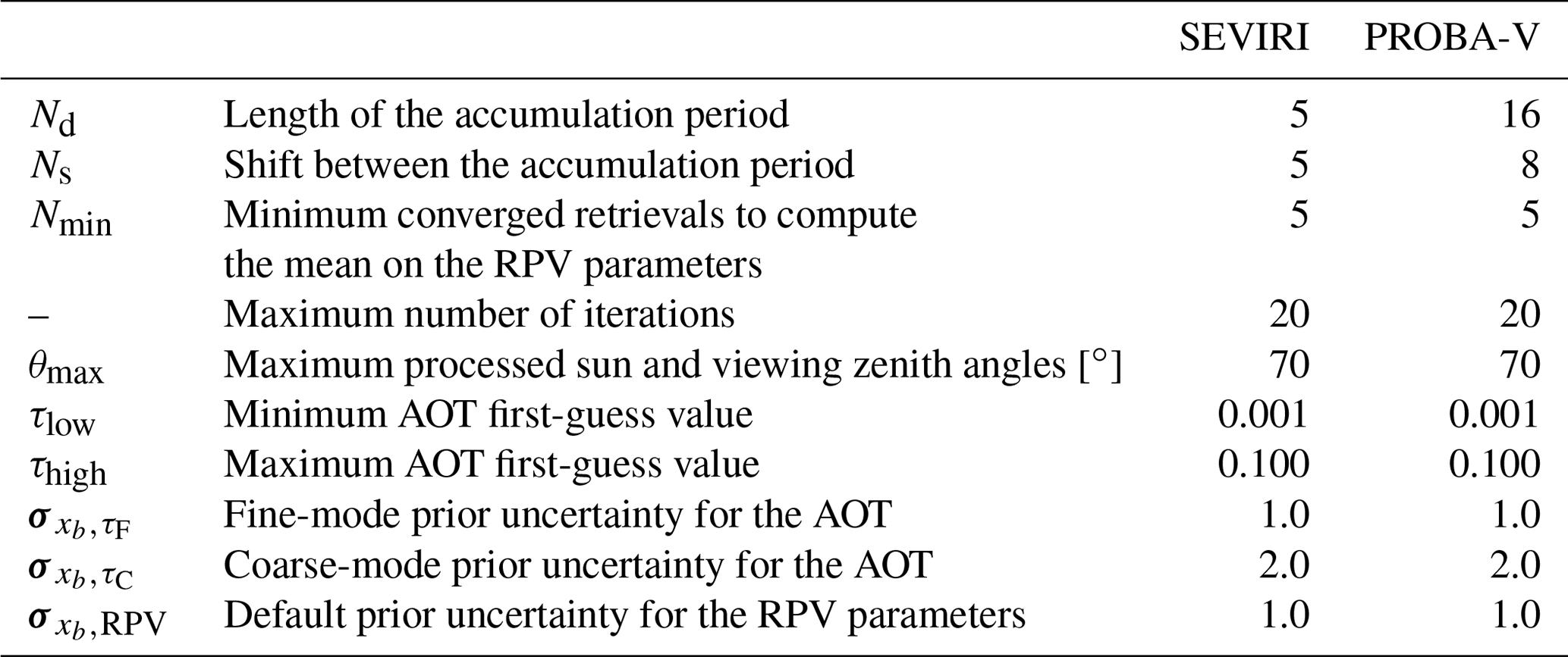
The definition of the first guess is an important aspect of the inversion process and it is defined in order to minimise the possibility of finding local minima. When a minimum value is found, an investigation of the cost function in the vicinity of the solution should be made in order to determine whether or not it is a local minimum. However, this exploration could be computationally expensive. In order to minimise the possibility of local minima without degrading the computational performances, the AOT first guess is assigned to successive observations alternating between a low-value τlow and a larger one τhigh (see Table 7). As CISAR retrieves a single set of RPV parameters over the entire accumulation period in each processed band, only one set of first guesses x0 is defined:
where is the index of the current accumulation period and xb is the prior information at the accumulation period td.
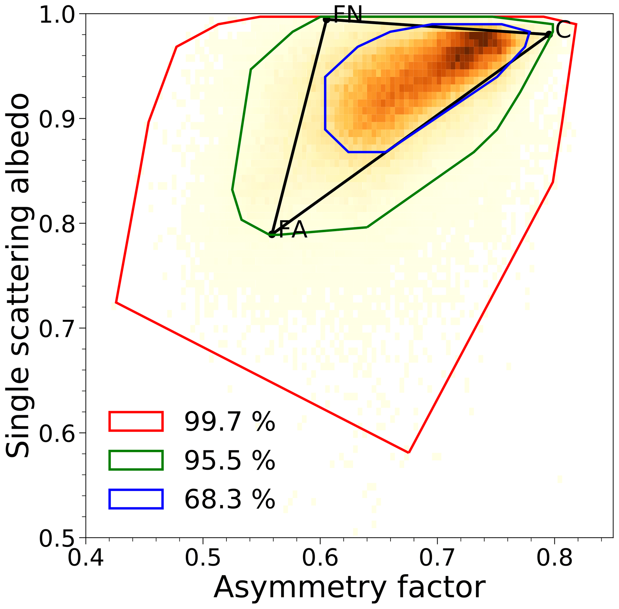
Figure 4Solution space (black triangle) for the wavelength 0.6 µm defined by the non-absorbing fine-mode (FN), the absorbing fine-mode (FA) and the coarse-mode (C) vertices. The red, green and blue lines show the 99.7 %, 95.5 % and 68.3 % probability regions respectively, derived from AERONET inversion product for all the observations available over all the AERONET stations.
From the retrieved set of RPV parameters the BHR is calculated, assuming perfectly diffuse illumination conditions, and the AOT is extrapolated at 0.55 µm through the extinction coefficient α:
where v is the considered aerosol vertex and λ is the wavelength from which the AOT at 0.55 µm is extrapolated.
3.2 Aerosol vertices
The aerosol vertices subsample the entire solution space to a region where the aerosol properties can be retrieved. The relationship between the particle size and the single-scattering properties has been discussed in Part 1. As recommended, three vertices are selected, defined by the asymmetry factor g and the single-scattering albedo (SSA) ω0: two fine-mode vertices, absorbing and non-absorbing, and one coarse-mode vertex, defining a triangle in the [g,ω0] space in each processed band. The three vertices are chosen to analyse the single-scattering properties derived from the AERONET inversion product on all available observations since 1993 (Dubovik et al., 2006), similarly to the approach proposed by Govaerts et al. (2010). The distribution of aerosol single-scattering properties in the [g,ω0] space, as derived from AERONET inversion product, is shown in Fig. 4 for λ=0.6 µm. The aerosol properties are clustered in the region defined by and , containing 68.3 % of the data (blue line). The selected CISAR vertices defining the solution space cover about 80 % of possible solutions (black triangle).
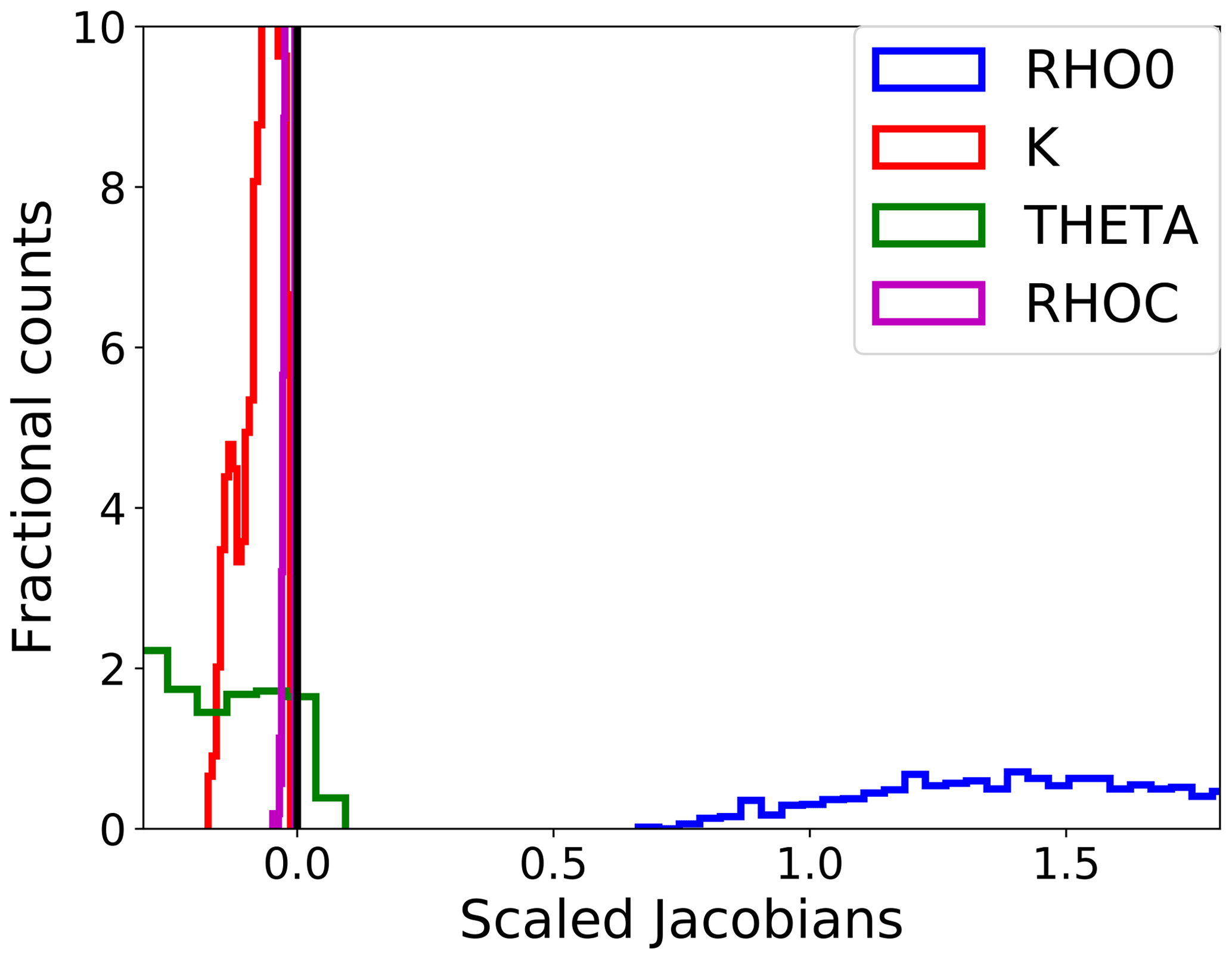
Figure 5Histograms of the distribution of the Jacobians related to the RPV parameters (x axis), scaled by the variability range of each variable. These distributions are obtained from PROBA-V observations (RED band) over Carpentras, France (vegetated target). Positive (negative) values of the Jacobian show that the TOA BRF is positively (negatively) correlated to the considered state variable.
The analysis of the information content relies on a two-fold approach. First, the Jacobians are used as an indicator of the TOA BRF sensitivity to state variable changes under different observation conditions. Next, the entropy is used as a rigorous metric to determine the information content of the observation system for each radiometer. The Jacobians, i.e. the partial derivatives of the forward model with respect to the state variables, are affected by the changes in illumination and viewing geometry both in terms of sign and magnitude (Luffarelli et al., 2016). The minimisation of the cost function relies on an iterative approach where the direction of steepest descent is determined by the Jacobians (Marquardt, 1963). An analysis of the Jacobians gives information about the amount of information carried by the observation and highlights variations in sensitivity throughout the year. The larger the magnitude of the Jacobians, the higher the sensitivity of the signal to the selected state variable. The Jacobians have been scaled by the variability range of each state variable to compare their dimensionless magnitude.
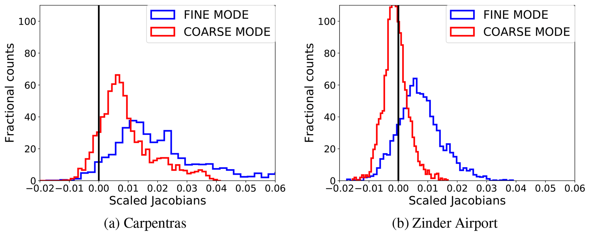
Figure 6Distribution of the AOT-scaled Jacobian over Carpentras (dark surface) and Zinder Airport (bright surface). The histograms are obtained from PROBA-V observations (RED band) over the year 2015.
Table 8Median and standard deviation of the scaled Jacobians. The table refers to all processed targets during 2015. The values are shown for the SEVIRI and PROBA-V bands centred at 0.6 µm.
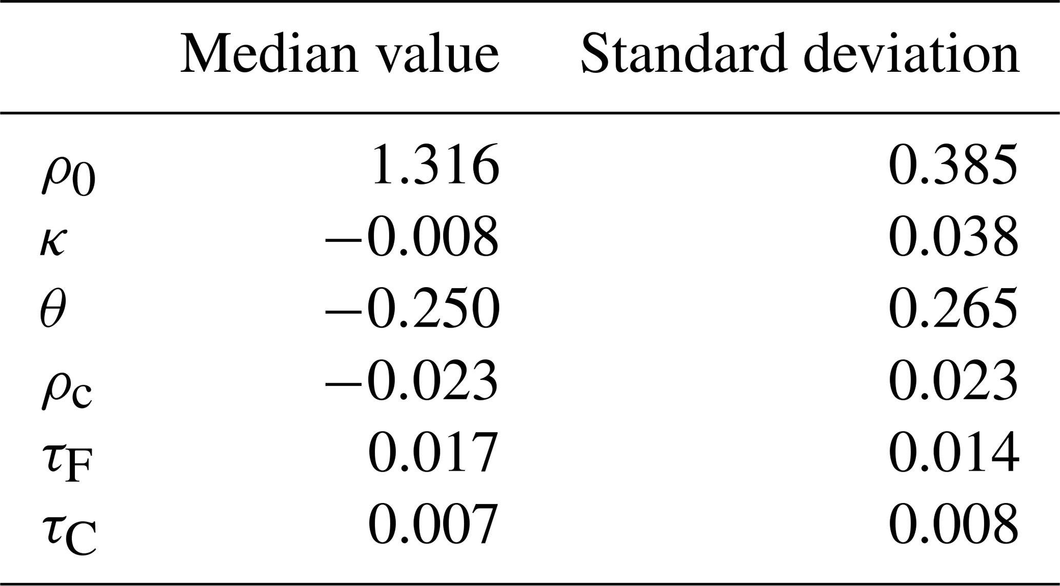
An illustrative example of the distributions of the Jacobians relative to the RPV parameters is shown in Fig. 5. The Jacobians are dominated by the ρ0 parameter (controlling the magnitude of the surface BRF), followed by θ, k and ρc (characterising the surface reflectance anisotropy). Consequently, the retrieval of the surface reflectance shape is more challenging than the retrieval of its mean magnitude; nevertheless, its accurate retrieval is necessary to correctly account for the coupling between the surface and the atmosphere (Govaerts et al., 2008).
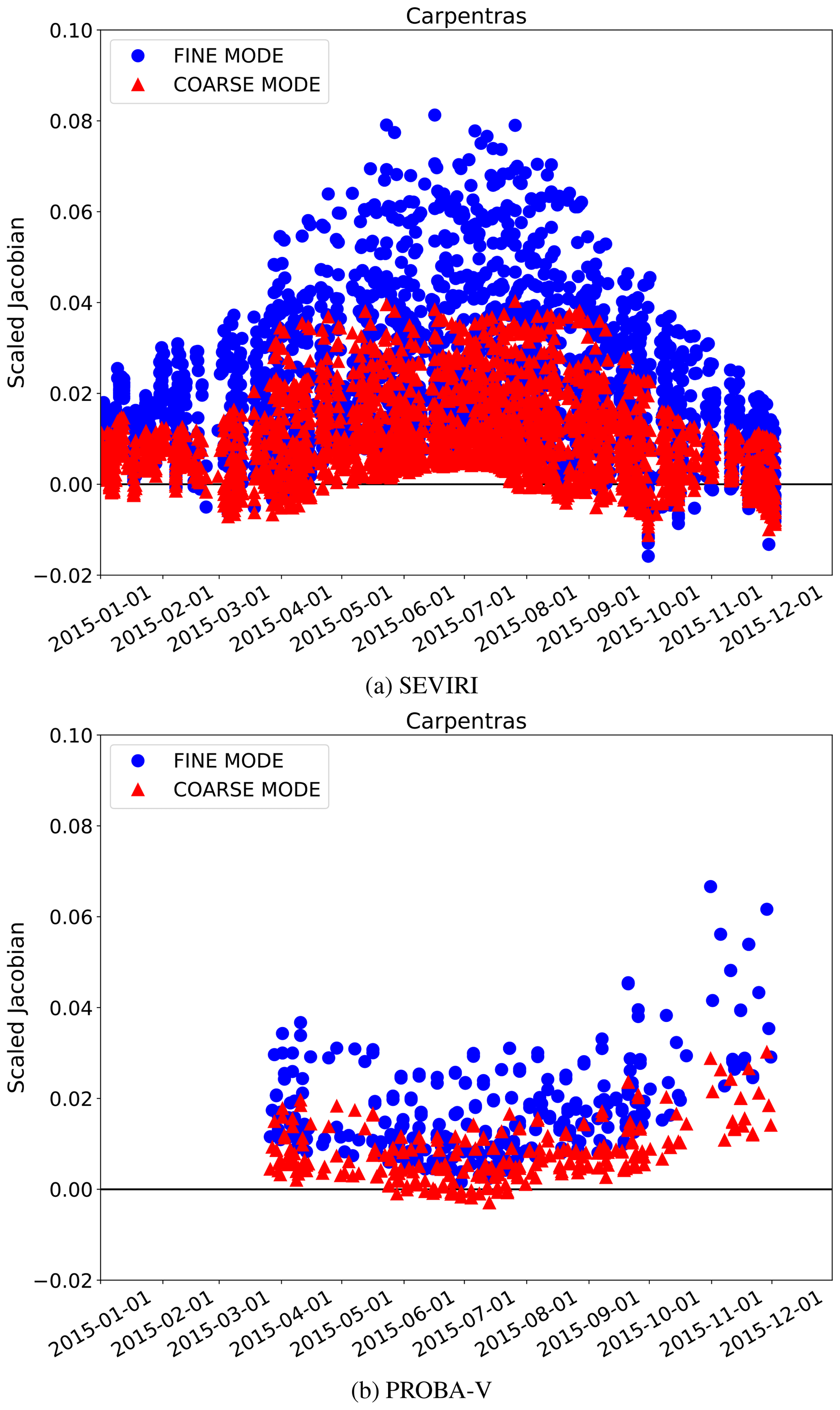
Figure 7Scaled AOT Jacobians time series over Carpentras, France (vegetated target) related to SEVIRI VIS0.6 band (a) and PROBA-V RED band (b) observations. The blue dots represent the fine mode and the red triangles the coarse mode.
The aerosol contribution to the TOA BRF differs according to the brightness of the surface. Figure 6 shows the AOT-scaled Jacobians distribution over Carpentras (dark surface) and Zinder Airport (bright surface). The Jacobians over Carpentras reach higher values with respect to the Jacobians related to Zinder Airport, because the signal at Zinder is dominated by the bright surface (Sun et al., 2016). When the magnitude of the AOT Jacobian is close to 0, the observed TOA BRF is not sensitive to changes in the aerosol concentration in the atmosphere. It is worth noting that the AOT-scaled Jacobians can be both negative and positive, meaning that the aerosols can increase or decrease the TOA BRF, depending on the season and the viewing and illumination geometry. This variability of the sign of the Jacobians, also occurring over dark targets (Fig. 6a), represents one limitation in the MODIS dense dark vegetation (DDV) algorithm (Kaufman et al., 1997), which assumes that an increase in the AOT results in an increased signal at the satellite.
Table 8 shows the median value and the standard deviation of the scaled Jacobians for all the state variables at SEVIRI and PROBA-V bands centred at 0.6 µm, over all selected AERONET stations. This table confirms the previous findings on the Jacobian magnitude shown in Figs. 5 and 6 over Carpentras and Zinder Airport. The AOT-scaled Jacobian is about 2 orders of magnitude smaller than that for the surface reflectance. The variability of the Jacobian sign and magnitude over the year is illustrated in Fig. 7, where it can be seen that the effect of the aerosols on the reflectance can vary with the geometry for the same land cover type. The Jacobian variations in Fig. 7 essentially depend on the viewing and illumination geometry. Aerosol particles mostly scatter in the forward direction, given the positive sign of the asymmetry factor g (controlled, among other factors, by the aerosol size distribution) (Andrews et al., 2006). For this reason, the maximum information on the aerosols is located in the forward direction, while it decreases when approaching the backscattering direction. Additionally, a longer atmospheric path increases the aerosol effects on the reflectance, given the higher probability of interactions between the reflected sunlight and the atmospheric particles. The impact of the length of the atmospheric path is highlighted in Fig. 8, showing the Jacobian daily cycle over Carpentras. The sensitivity of the TOA BRF with respect to the AOT almost disappears at noon, when the atmospheric path is shortest and the effect of the aerosols on the signal is minimised. A more detailed analysis of the AOT Jacobians and their relation with the AOT magnitude is performed by Luffarelli et al. (2016). Given the seasonal variations of the Jacobians shown in Fig. 7 and 8 it is not expected that the same accuracy of the retrieval will be obtained throughout the day and throughout the year.
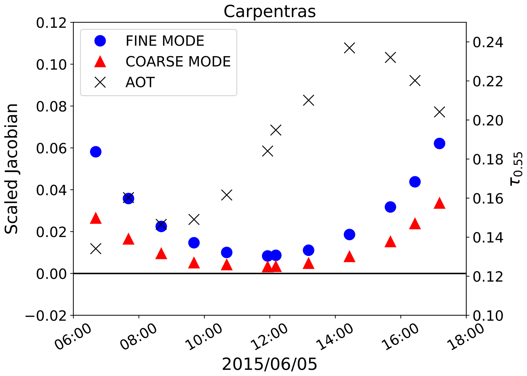
Figure 8Scaled AOT Jacobians (left y axis) associated with SEVIRI observation in the VIS0.6 band over Carpentras, France, for 5 June 2015. The blue dots represent the fine mode, the red triangles the coarse mode. The black crosses represent the retrieved AOT at 0.55 µm (right y axis).
A more rigorous analysis of the information content can be made through the entropy, which measures the uncertainty reduction (Rodgers, 2000). In an OE framework, the prior information and its uncertainty represent a hypothesis on the expected value of the state variables. It is envisaged that the inversion process provides a posterior uncertainty on the state variables which is smaller than the prior one; the entropy quantifies this uncertainty reduction. When there is no information coming from the satellite observations, the entropy will be close to 0 as the observation does not add any knowledge to the system. Formally, the entropy is computed as follows:
where (Eq. 21 of Part 1) and Sx are the uncertainties in the posterior and the prior information.
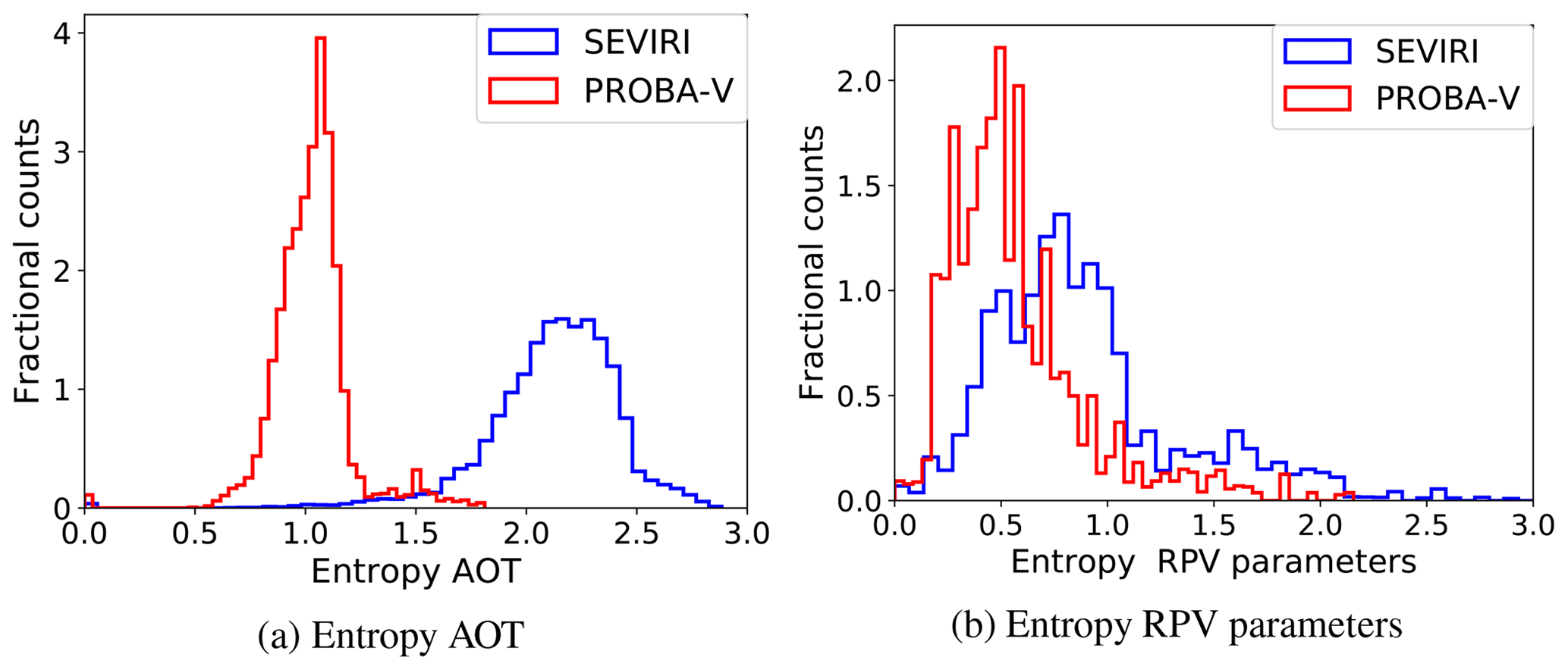
In CISAR, the entropy is calculated considering the surface and atmospheric state variables and their associated prior and posterior uncertainty separately; the entropy distribution is shown in Fig. 9. The distribution of the surface and AOT entropy related to SEVIRI observations exhibits higher values compared to the one related to PROBA-V observations, given the larger radiometric uncertainty associated with the observations acquired by the polar-orbiting satellite. The entropy not only depends on the information carried by the satellite observation, but also on the uncertainty associated with the prior information. As the prior information on the surface is updated (Sect. 2.4), the associated uncertainty decreases in time, whereas the prior information on the AOT remains weakly constrained, as the uncertainty is kept to the default high value. For this reason, the entropy associated with the RPV parameters a exhibits smaller value than the one associated with the AOT (Fig. 9a).
5.1 Review of existing methods
Section 2.5 discussed the limitations of the forward model FASTRE. Furthermore, in Sect. 4 it has been shown that the AOT Jacobian magnitude is subject to temporal variations depending on the viewing and illumination geometries. These issues compromise the reliability of the retrieved solution, which can be assessed using different methods. Dubovik et al. (2011) use the relative fitting measurement residual to filter the retrieval outliers. This approach presents some limitations as the number of degrees of freedom can vary depending on the availability of cloud-free observations. The requirement for the quality of the fit should be stricter when only a limited number of observations are available (Govaerts et al., 2010). This specific issue was addressed in Govaerts and Lattanzio (2007), who developed an approach which also takes into account the number of cloud-free observations. The authors observed that the cost function is proportional to the quadratic sum of the mismatch between the simulation and the observation for each acquisition, weighted by the observation uncertainty. As the cost function is strongly dependent on the number of observations, it is not possible to define a universal range of acceptable values for its residual without performing additional operations on the cost function. Both methods do not correctly identify situations in which a good fit is reached, but the retrieval of the state variables is not reliable due to limited or no dependency of the TOA BRF on the state variables (the Jacobians are close to 0). A more elaborate QI has been developed for the MODIS Aerosol Product Collection 6 (Hubanks, 2017), which is composed of different tests accounting for the fitting residual, the magnitude of the retrieved AOT, the possible presence of cirrus, the brightness of the scene and information on the number of pixels and the percentage of water pixels present in the processed area. Despite taking into account different factors in addition to fitting residuals, this approach does not consider the actual information content of the satellite observation. Moreover, as CISAR processes each pixel independently, the information on the number and type of pixels over which the retrieval is performed, as used in the MODIS product, is not applicable within this method.
5.2 Overview
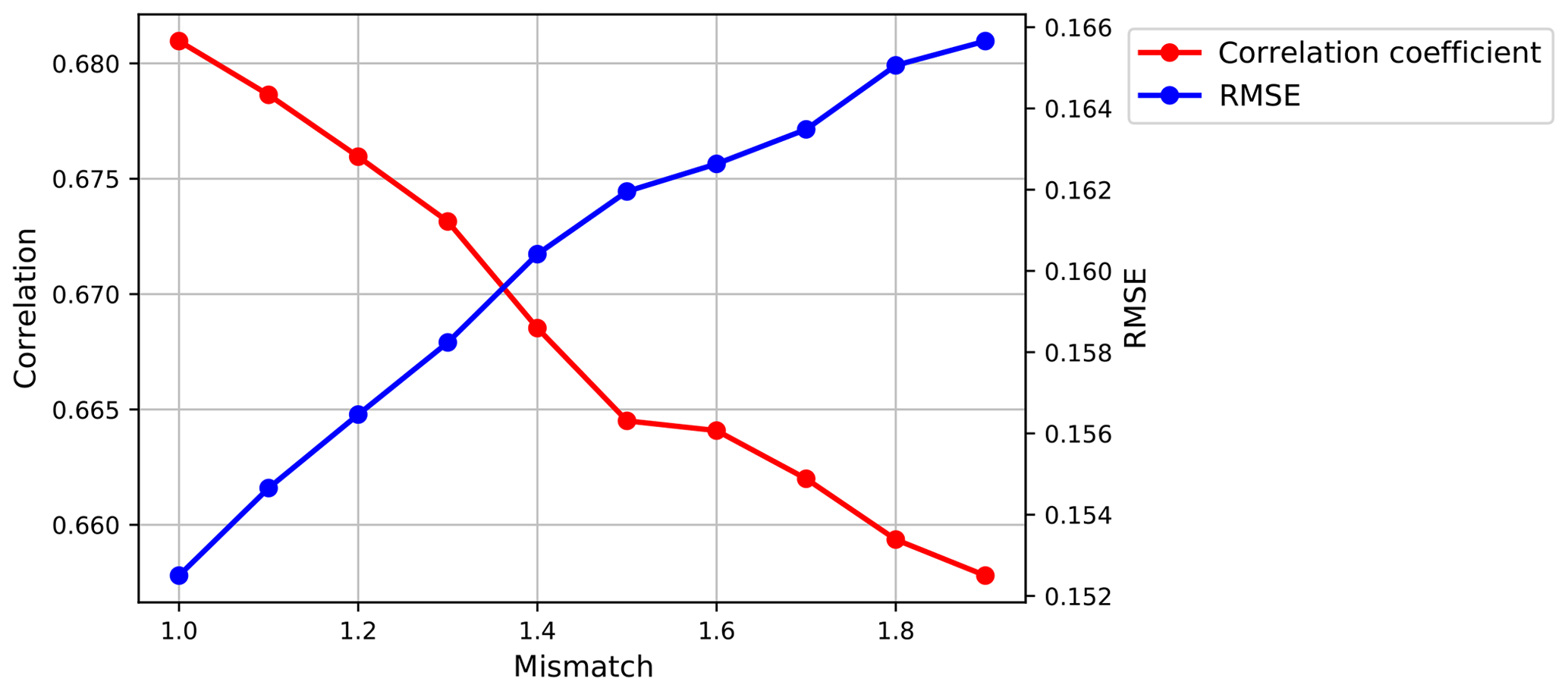
Figure 10Correlation (in red) and RMSE (in blue) variations as a function of the mismatch between the satellite observation and the simulated signal (test 3). The figure refers to the CISAR AOT retrieval evaluation against AERONET data. These results are obtained from CISAR applied to SEVIRI observations.
A new approach is proposed for the CISAR algorithm, which combines a series of individual tests j with an associated value pj in the range [0,1], defining a QI(ti) associated with the solution retrieved at the time ti. These tests evaluate the convergence of the inversion to a solution after a given number of iterations (0), on the validity range of the total AOT (1) and surface albedo (2), on the mismatch between observations and simulations (3) and on the information content of the satellite acquisition through the Jacobians (4) and the entropy, as discussed in Sect. 4. The entropy is computed separately for the AOT (5) and RPV parameters (6). These tests have been defined through an analysis of their impact on the CISAR performance when evaluated against independent reference data sets. The value pj associated with each test can assume values between 0 (bad quality) and 1 (good quality). Figure 10 shows an example of the evaluation of the retrieved AOT against the AERONET data for the mismatch test (3). As the mismatch increases, the correlation decreases, while the root mean square error (RMSE) shows the opposite behaviour.
5.3 Quality indicator tests
5.3.1 Convergence
The first test to be performed is on the convergence of the inversion. When the maximum number of iterations is reached, p0 is equal to 0, otherwise p0=1.
5.3.2 State variable validity range
The validity of the retrieved total AOT and of the surface BHR is examined in tests 1 and 2. In CISAR, a validity range for each state variable is defined, based on physical boundaries and empirical observations. When the value of retrieved AOT (BHR) falls at the extremes of this range, p1 (p2) is equal to 0. The acceptable values for the BHR range from 0 to 1, while the AOT can only assume positive values smaller than 5. The values p1 and p2 are equal to 1 when 0< BHR <1 and 0< AOT <5 respectively.
5.3.3 Mismatch between observation and simulation
As discussed in Sect. 5.1, the fitting residual between the observation and the simulation is normally used to assess the reliability of the solution, as it describes how well the signal simulated with the forward model ym(ti,λ) fits the satellite observations y0(ti,λ). The mismatch between the observed and simulated TOA BRF is weighted by the observation's uncertainty σ0(ti,λ). For this test, the largest mismatch among the processed bands is considered. Two thresholds, T1 and T2, are defined to identify good (p3=1) and bad (p3=0) quality retrievals. The difference between the simulated signal and the satellite observation should have the same magnitude as the observation uncertainty σ0(ti,λ); therefore T1 is set to 1. Conversely, the maximum acceptable mismatch value T2=2 has been chosen by observing the relationship between the mismatch and the performances of CISAR when evaluated against the independent data sets used for reference. Fig. 10 represents an example of this analysis. When the mismatch assumes values within the range defined by T1 and T2, thresholds included, a value between a minimum m and 1 is assigned to p3 through a sigmoid function with width equal to (Fig. 11). A different coefficient m is defined for each test j in order to give different weights to the tests, according to the magnitude of their impact on the retrieved solution and its evaluation against the reference data set. The outcome of test 3 is thus defined as follows:
with λ=1, …, number of wavelengths.
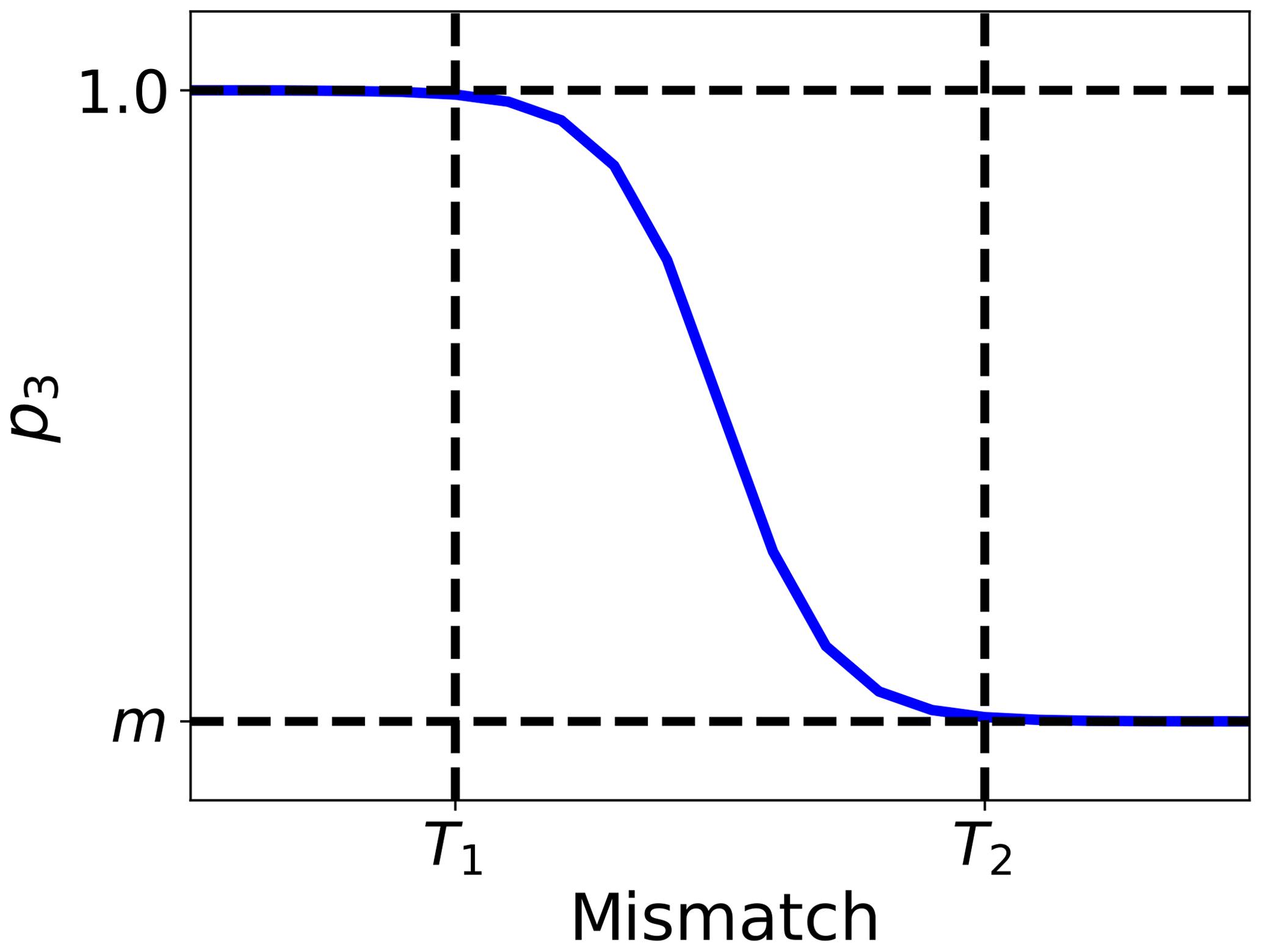
Figure 11Non-linear p3 definition between the minimum value m and 1, which applies when the mismatch is larger than T1 and smaller than T2.
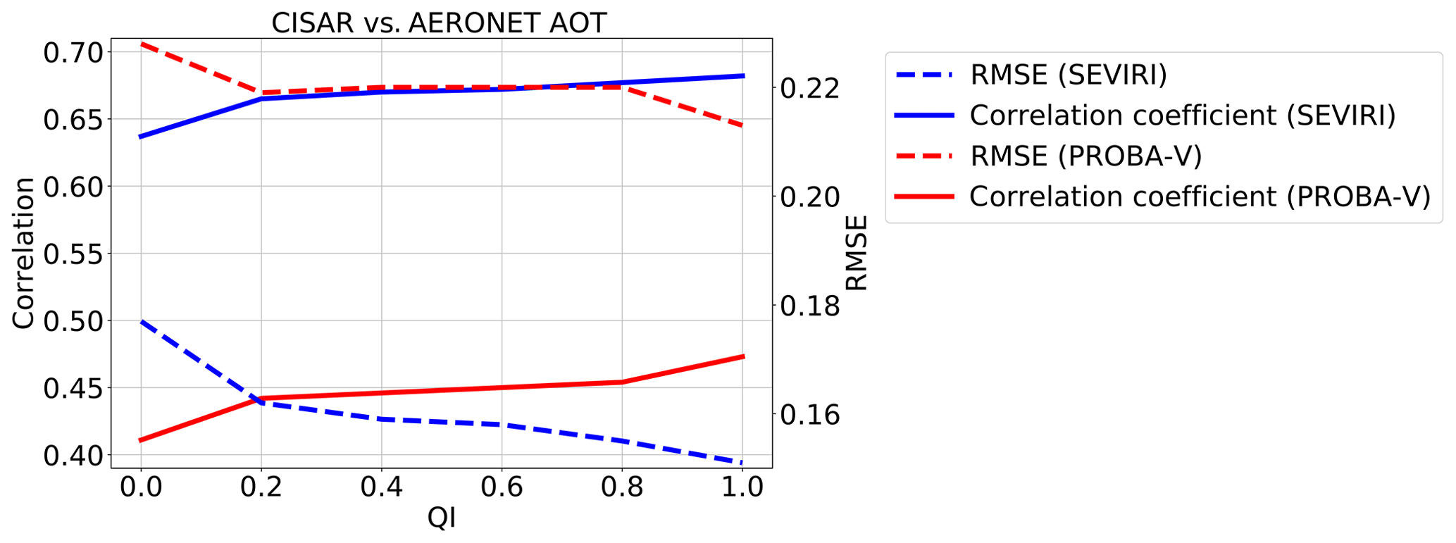
Figure 12Correlation (straight lines) and RMSE (dashed lines) variations as a function of the QI. The figure refers to the CISAR AOT retrieval from SEVIRI (in blue) and PROBA-V (in red) observations evaluated against AERONET data. The QI is rounded to the nearest 0.1.
Table 9CISAR-retrieved BHR from comparison of actual observations with MODIS in all the processed bands.
5.3.4 Jacobians
The magnitude of the Jacobians gives information on the sensitivity of the TOA BRF to the state variables. Performing a test on the Jacobians related to each state variable can be computationally expensive. In order to reduce the computational effort, only the Jacobian of the AOT is taken into account. The spectral constraints applied to the AOT variability as in Sect. 2.4 impose a correlation between the AOT retrieved in the different spectral bands. Consequently, it is desirable to have large absolute Jacobians in at least one band. To have a good retrieval of the total AOT, the AOT associated with each aerosol vertex has to be correctly retrieved. The quantity analysed in test 4 is thus the following:
with λ=1,…,number of wavelengths and v=1, …, number of aerosol vertices.
The aim of this test is to discard observations with little or no sensitivity to the AOT and to identify those situations in which the test on the misfit is successful because of the prior information and/or the temporal and spectral constraints (Sect. 2.1) rather than actual information coming from the observations. The thresholds T1 and T2 are set to 0.01 and 0.02 respectively. The values of p4 are defined similarly to p3:
5.3.5 Entropy
Section 4 discusses how the entropy, which quantifies the uncertainty reduction from the prior knowledge on the system to the posterior uncertainty, represents a rigorous analysis of the information content. Tests 5 and 6 analyse the entropy associated with the AOT and the one associated with the RPV parameters, computed as follows:
where Nλ is the number of processed wavelengths, λ=1, …, Nλ, p=1, …, number of RPV parameters and v=1, …, number of aerosol vertices. The normalisation to Nλ ensures consistency in the entropy evaluation when different number of bands are analysed, as for the SEVIRI and PROBA-V cases. The entropy computation is strongly dependent on the magnitude of the prior uncertainty as explained in Sect. 4. Low entropy might be due to reliable prior information, with a low associated uncertainty. Similarly, the uncertainty reduction would be very large in the case of little prior information on the state variable. For these reasons, tests 5 and 6 are only performed when the prior uncertainty is smaller than the validity ranges of the AOT and RPV respectively and larger than one-sixth of it. The thresholds associated with the two tests on the entropy are T1=0.1 and T2=0.6, which correspond to a 20 % and 70 % uncertainty reductions respectively. The values p5(ti) and p6(ti) are computed as in Eq. (15).
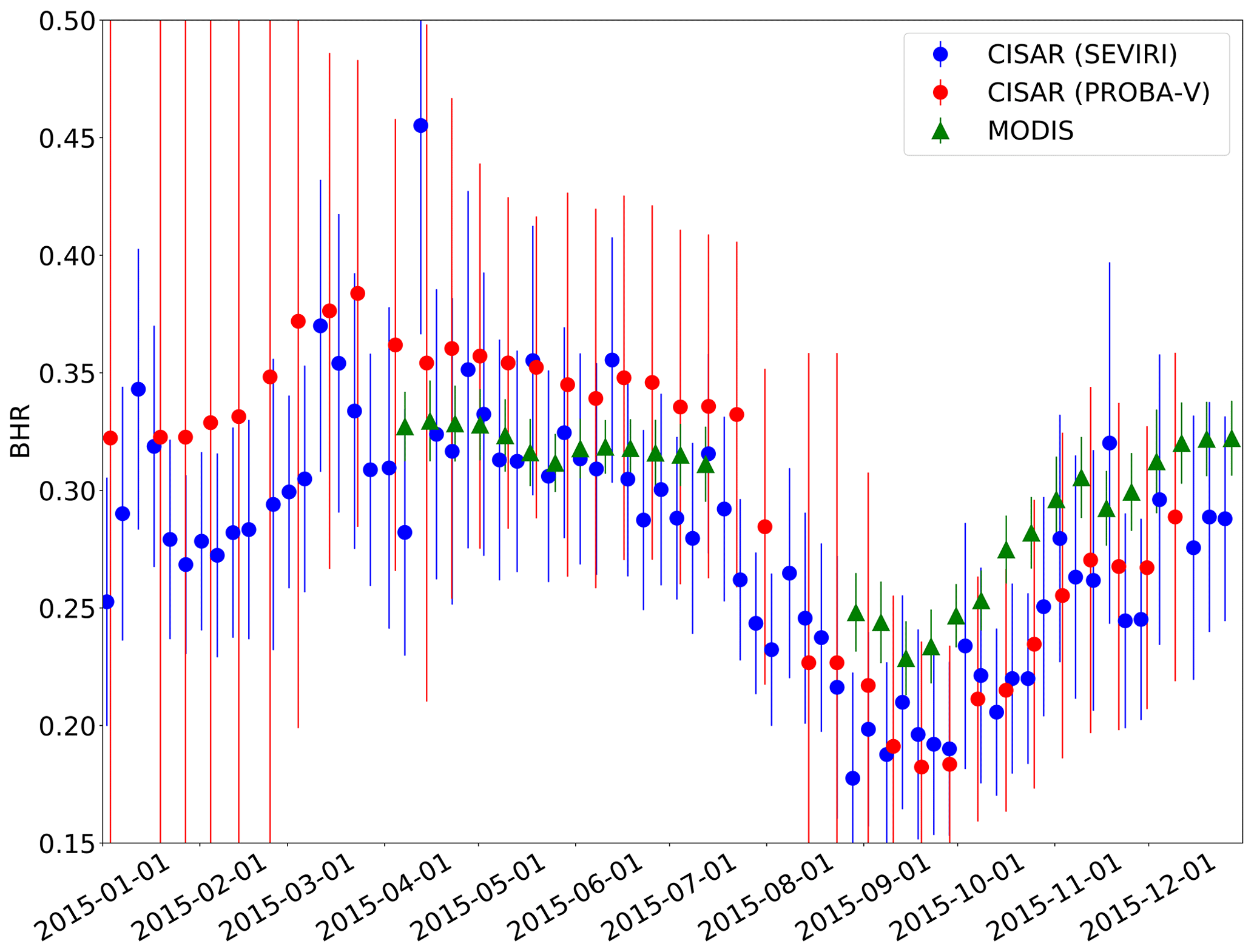
Figure 13CISAR-retrieved BHR from SEVIRI (blue dots) and PROBA-V (red dots) and MODIS land product (green triangle) over Zinder Airport (Niger, Africa). The results are shown for each sensor's band centred at 0.6 µm for the year 2015. The vertical bars represent the retrieval uncertainty for SEVIRI and PROBA-V and standard deviation over the selected area for MODIS.
5.4 Quality indicator computation
The final QI is computed by combining the results of the tests performed on the retrieved solution:
The final QI(ti) ranges from 0 to 1, where 0 designates a poor-quality retrieval and 1 indicates a reliable solution. Figure 12 shows the variations of the correlation and the RMSE between CISAR-retrieved AOT and AERONET data as a function of the QI. The correlation increases as the QI takes larger values, while the RMSE decreases. This behaviour is observed with CISAR AOT retrieved from both SEVIRI and PROBA-V observations (Fig. 12). This correlation increase (RMSE decrease) is particularly visible when QI is taking values between 0.0 and 0.2. For this reason, only retrievals with QI ≥0.2 are considered in Sect. 6.
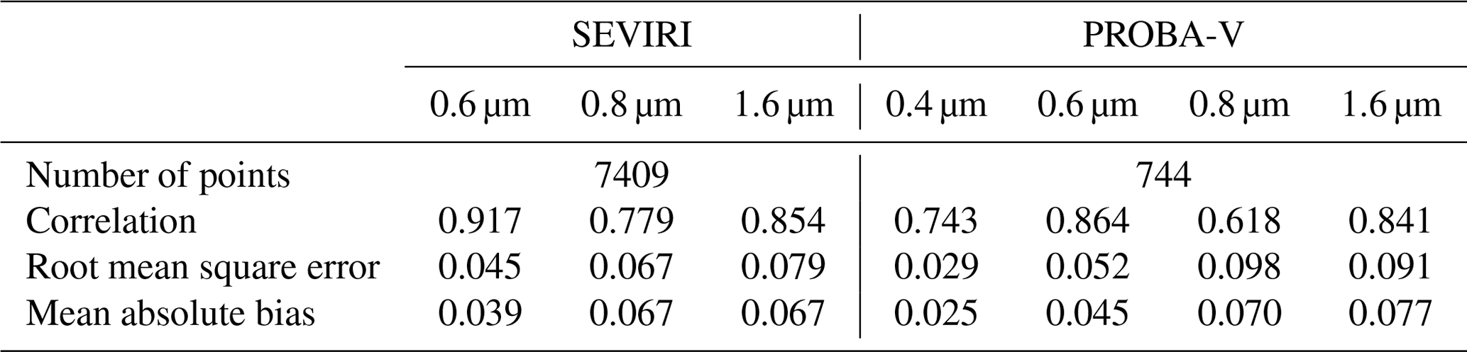
6.1 BHR
The CISAR BHR, computed from the RPV parameters, is compared with the MODIS land product (Schaaf and Wang, 2015). To account for the different spatial sampling, the MODIS data have been averaged on 5×5 km and 1×1 km for the comparison with the retrievals from SEVIRI and PROBA-V respectively. The results of this comparison are shown in Table 9 in terms of correlation, RMSE and mean absolute error (MAE). The CISAR results show a high correlation with the MODIS product, above 0.7 in all the processed spectral bands, except the PROBA-V NIR band, which shows a correlation of 0.618. The density plots of the CISAR BHR retrievals against MODIS data are included in the Supplement for all the processed bands, for both satellites. Despite the instrument differences discussed in Sect. 2.5, the CISAR retrievals and the MODIS land product show similar seasonal trends. Figure 13 shows the BHR time series over Zinder Airport (Niger, Africa), as retrieved from the CISAR algorithm applied to SEVIRI and PROBA-V observations and from the MODIS land product. The rainy season, from 20 May to 5 October (Weatherspark.com, 2018), is distinguishable through the decrease in the surface BHR in both the MODIS and CISAR data sets, although CISAR retrieves a larger seasonal variation with respect to MODIS product. The effect of the updating mechanism on the surface prior described in Sect. 2.4 is also visible as the retrieval uncertainty decreases in time, given that the prior information on the surface is better defined.

Figure 14Box plots showing the CISAR AOT retrieval extrapolated at 0.55 µm (left y axis) against the AERONET data (x axis) for SEVIRI (a) and PROBA-V (b) over all the selected stations. Only retrievals with QI ≥0.2 are considered. The blue boxes represent the interquartile range (IQR), the red horizontal line represents the median value, the vertical dashed bars represent the 1.5× IQR range and the black crosses represent the outliers. Boxes with fewer than 10 points are not displayed. The green histograms represent the AERONET AOT distribution. The right y axis shows the percentage of points contained in each bin.
6.2 Aerosol optical thickness
The CISAR AOT retrieval, extrapolated at 0.55 µm, has been evaluated against the AERONET data over the selected targets listed in Sect. 2. The CISAR AOT retrieval is evaluated in terms of correlation, RMSE and MAE with respect to AERONET values. Additionally, the percentage of points falling within the Global Climate Observation System (GCOS) requirements (Systematic Observation Requirements for Satellite-Based Data Products for Climate, 2011 Update), defined as , is also accounted for. The GCOS requirements are a useful tool for comparing different algorithms' performances. However, both the SEVIRI and PROBA-V missions were not originally designed for AOT retrieval. The GCOS requirement of 0.03 for low optical thickness translates into a radiometric noise requirement much better than 2 (1) % at 0.4 (0.6) µm, well below the radiometric performance of the SEVIRI and PROBA-V instruments (Table 3). The duration of the corresponding missions, however, provides a decisive advantage for the generation of AOT data sets from these instruments. In the following, the GCOS requirements are evaluated in terms of percentage of retrievals satisfying them.
Figure 14 shows the evaluation of the retrieved AOT against AERONET data for both SEVIRI (left panel) and PROBA-V (right panel). The CISAR retrievals from SEVIRI observations show a better agreement with the AERONET data compared to the retrievals from PROBA-V observations. This is in accordance with the poor radiometric performances of the polar-orbiting instrument and with the outcome of the information content analysis performed in Sect. 4.
The box plots in Fig. 14 show an overestimation of the retrieval for low AOT and an underestimation for large AOT. Similar behaviour is also observed in Wagner et al. (2010). The underestimation of large values might be partially due to the temporal constraints described in Sect. 2.4, as they might prevent the algorithm from fitting rapidly evolving aerosol events associated with large AOT values. However, the applied temporal constraints are intended to optimise the retrieval of low aerosol concentration, given the global distribution of AOT, which is normally smaller than 0.2 (Kokhanovsky et al., 2007). Additionally, very high AOT normally corresponds to local events, especially in Europe (e.g. plume, fire); therefore the AOT obtained by the retrieval from the satellite pixel containing the AERONET station will be lower than the one measured by the AERONET tower (Jiang et al., 2007). The histograms in Fig. 14 show that AOT values larger than 0.8 represent less than 5 % of the total number AERONET observations, affecting the reliability of the statistics for high values of AOT. The processing of more data would be necessary to increase the confidence in the results for high AOT values. Some examples of CISAR's ability to detect high AOT are shown in the Supplement.
The overestimation of low AOT might originate from the different spatial scales of the satellite observations and the ground measurements. Most of the selected AERONET stations are located in Europe (Fig. 1), where the SEVIRI pixel resolution is about 5×8 km (as opposed to 3×3 km at the subsatellite point), which is compared to AERONET point measurement. The probability of residual cloud contamination on this scale might thus explain part of the overestimation (Henderson and Chylek, 2005, Chand et al., 2012). Furthermore, the shortest SEVIRI spectral band is centred at 0.67 µm, where the sensitivity to low optical thickness is about 2 times smaller than in the blue spectral region. Consequently, the retrieval in these cases essentially relies on the prior information regardless of the very large associated uncertainty. Despite the presence of a blue band and a better spatial resolution (1 km), the retrievals from PROBA-V observations still show an overestimation at low AOT due to the poor radiometric performances which decrease the importance of the information derived from the observations and the lack of a thermal channel that leads to an unreliable cloud mask.
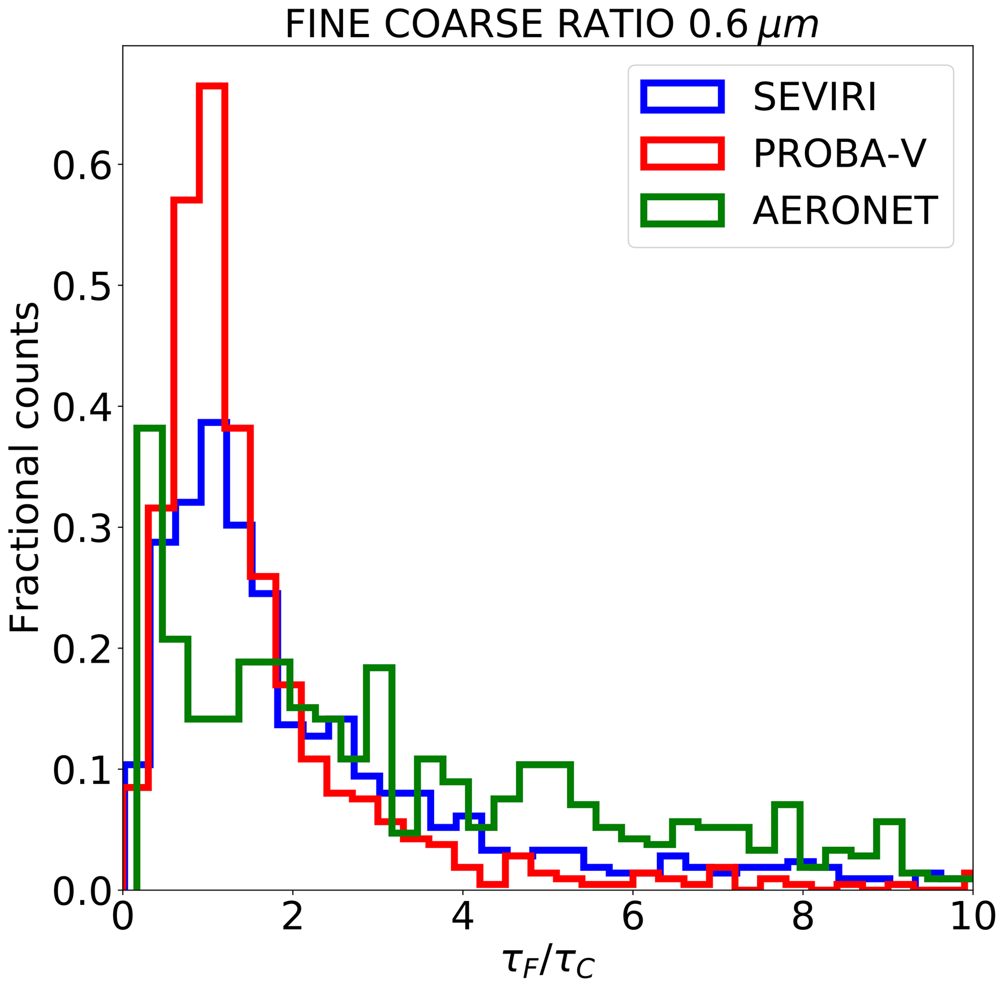
Figure 15Fine- to coarse-mode ratio distribution at 0.6 µm from AERONET (green) and from CISAR applied to SEVIRI (blue) and PROBA-V (red) observations.
The CISAR potential to discriminate between the fine and coarse mode is analysed next. Figure 15 shows the fine- to coarse-mode ratio distribution related to AERONET data (in green) and CISAR retrieval for SEVIRI (in blue) and PROBA-V (in red). It can been seen that the distribution related to CISAR retrievals from SEVIRI and PROBA-V observations underestimate the fine-mode concentration for . The percentage of cases where CISAR succeeds in retrieving a predominantly fine-mode contribution to the total AOT () is equal to 80 % when the retrieval is performed on SEVIRI acquisition and 62 % when CISAR is applied to PROBA-V data. This represents an improvement with respect to the land daily aerosol (LDA) algorithm (Wagner et al. (2010), Table 4), where particles retrieved by AERONET as spherical were correctly characterised by the algorithm in only 12 % of cases. This represents a decisive advantage of the proposed approach with continuous variations of the aerosol properties in the solution space, as opposed to the use of a limited number of aerosol classes, as in Wagner et al. (2010). The coarse-particle retrieval appears to be more challenging for both satellites. The percentage of cases where the coarse mode is correctly retrieved as predominant are 43 % and 30 % for the retrievals from SEVIRI and PROBA-V observations. The less accurate retrieval of the coarse mode compared to the fine mode is expected, as the considered wavelengths are less sensitive to the radii in the range of the coarse particles than to those of fine ones (Torres et al., 2017). This can also be observed in Table 8, where the median magnitude of the coarse-mode Jacobian is less than half of the fine-mode Jacobian.
6.3 Single-scattering albedo and asymmetry factor
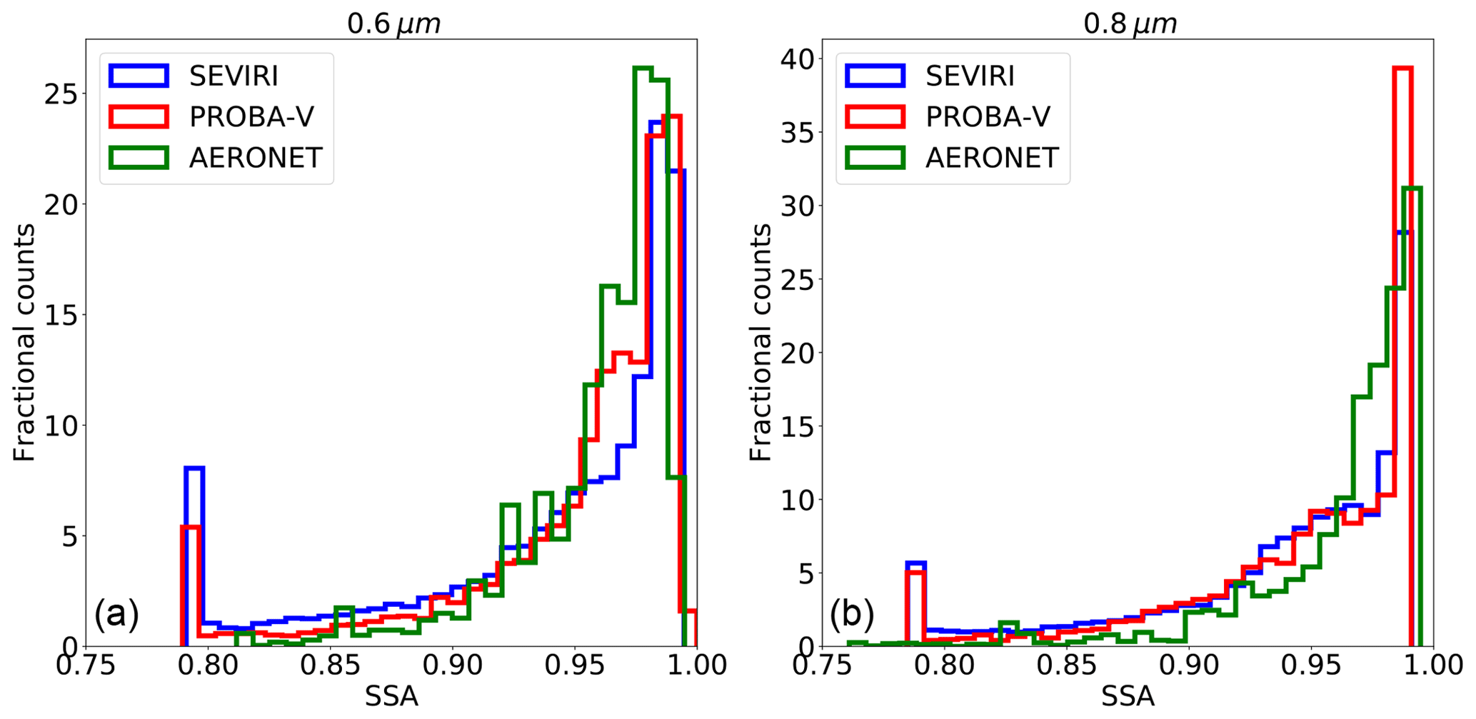
Figure 16SSA distributions at 0.6 µm (a) and 0.8 µm (b) for AERONET (green), and CISAR applied to SEVIRI (blue) and to PROBA-V (red).
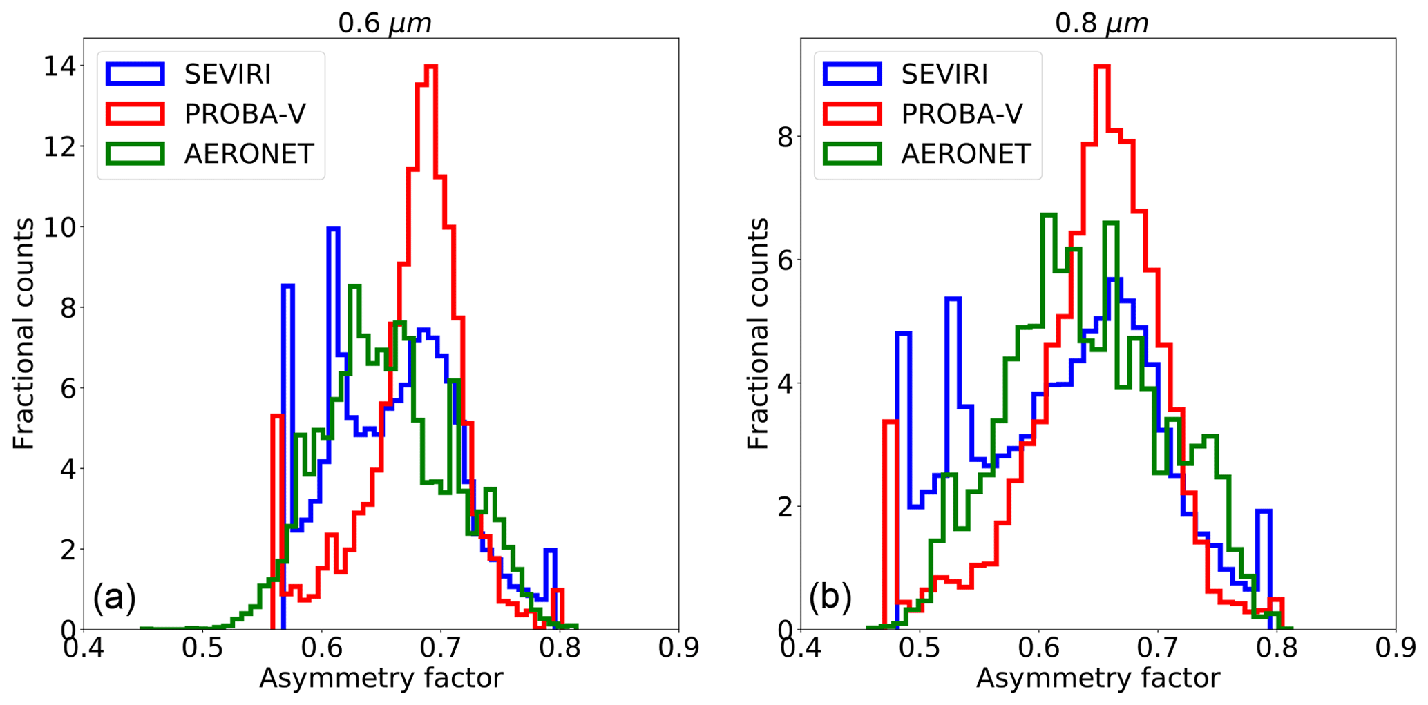
In Sect. 3.2 the solution space defined by the aerosol classes vertices has been described. CISAR retrieves the averaged SSA and asymmetry factor within this solution space as linear combinations of the single-scattering properties of each selected aerosol vertex (Eqs. 8 and 9 of Part 1). Figures 16 and 17 show the SSA and asymmetry factor distributions related to the AERONET inversion product and CISAR retrievals. All the AERONET inversions are considered without applying the quality test as in Holben et al. (2006). The three data sets show similar distributions, although spikes can be observed at the extremes of the CISAR retrieval distributions. When the AERONET solution is located outside the solution space, CISAR cannot converge to it and the retrievals fall on the solution space boundaries, causing the spikes. The aerosol vertices selection in Fig. 4 is conceived to limit the number of occurrences of these spikes. Figure 17 shows that the g parameter distributions obtained from PROBA-V observations is much narrower than the same distribution related to AERONET and CISAR applied to SEVIRI observations. This is in line with what has been discussed in Sect. 6.2 on the poorer CISAR performances in retrieving the predominant mode when applied to PROBA-V observations rather than the SEVIRI ones. In fact, when computing g, the aerosol size distribution is the most important parameter to measure (Andrews et al., 2006), an inexact estimate of the dominant mode (fine or coarse) leads to an erroneous measurement of the asymmetry parameter.
This paper describes and evaluates the application of the CISAR algorithm to satellite observations acquired from geostationary and polar-orbiting instruments. The theoretical aspects of CISAR, a new generic algorithm for the joint retrieval of surface reflectance and aerosol properties, with continuous variation of all the state variables in the solution space, are described in Part 1. In the latter, CISAR is applied to simulated noise-free observations in the principal plane. This paper provides an evaluation of the algorithm in non-ideal situations, i.e. actual satellite observations acquired from both geostationary and polar-orbiting satellites, namely SEVIRI and PROBA-V.
The proposed retrieval method relies on an OE approach which consists of the inversion of FASTRE, a simple radiative transfer model composed of two horizontal layers. The FASTRE model is evaluated in Sect. 2.5 showing an accuracy within 3 % when compared to a complex 1-D radiative transfer model. Higher uncertainties are observed in spectral bands affected by water vapour as a result of the limited vertical discretisation.
The analysis of the information content of the satellite observations is performed in Sect. 4. Though the PROBA-V instrument has one blue channel, which is not present in SEVIRI, the better radiometric performances of the geostationary satellite provide more information on the retrieval of surface reflectance and aerosol properties than the polar-orbiting instrument.
The CISAR retrieval is evaluated against independent data sets. The retrieved AOT is compared to AERONET data. A specific QI has been developed to disregard suspicious retrievals. With an RMSE of 0.162 for SEVIRI and 0.176 for PROBA-V, CISAR shows better performances when applied to the geostationary satellite. CISAR retrieves the single-scattering aerosol properties, assuming a linear behaviour of g and ω0 in the solution space; although this assumption is not exactly true when far from pure single-mode situations, CISAR-retrieved aerosol properties distributions are in good agreement with the AERONET inversion products, especially when the algorithm is applied to geostationary observations, as discussed in Sect. 6.3. These differences are explained by the different information content associated with the observations acquired by the two satellites. For both satellites, the CISAR discrimination between fine and coarse mode is improved with respect to the LDA algorithm (Wagner et al., 2010), as the continuous variation of the aerosol properties in the solution space allows more accurate retrievals of the single-scattering properties with respect to that LUT-based approach. The CISAR surface albedo is compared with the MODIS product, showing a correlation higher than 0.74 in all processed bands (with the exception of the NIR PROBA-V band). The better performances of CISAR in retrieving the surface reflectance rather than the AOT are explained by the larger contribution to the TOA BRF of the surface. The small variance of surface reflectance on a short timescale allows a good prior definition based on the previous CISAR retrievals.
Several aspects of the new CISAR algorithm would still require additional effort to improve its performance. The analysis of the Jacobian median values has revealed the very small magnitude of the fine- and coarse-mode AOT Jacobians. The spectral and temporal constraints of the AOT variability play a critical role in supporting the assessment of aerosol properties. However, these constraints might lead to an underestimation of the AOT for large values. The impact of cloud mask omission errors on the AOT overestimation at low optical thickness deserves additional work. In order to reduce the impact of cloud contamination in the AOT retrieval, a new version of the CISAR algorithm is under development in the framework of the ESA-SEOM ConsIstent Retrieval of Cloud Aerosol Surface (CIRCAS) project (http://www.circas.eu/, last access: 21 Janaury 2019). The new version of CISAR aims to retrieve both the AOT and the cloud optical thickness (COT), overcoming the need for an external cloud mask. Within the CIRCAS project, CISAR will be applied to observations acquired by the Sea and Land Surface Temperature Radiometer (SLSTR) on board Sentinel-3.
As pointed out in Part 1, the limited number of state variables retrieved by CISAR allows the same algorithm to be applied to sensors which have not been originally designed for aerosol or surface albedo retrieval. The possibility to apply the same algorithm to data acquired by different instruments for the retrieval of several essential climate variables (ECVs) presents a decisive advantage, as it provides radiatively consistent ECVs derived from different sensors. Conversely, the use of separate methods for the retrieval of different variables might lead to a radiance bias, which has to be corrected before the assimilation of these variables (Thépaut, 2003). The effort for the assimilation of surface and atmospheric products could be reduced if the different ECVs were consistently derived with one single algorithm. The consistent retrieval of the state variables and the algorithm applicability to different sensors represent an important advantage for the numerical weather prediction (NWP) community, whose the main future challenges are related to a more consistent retrieval of Earth's system components and to the availability of more satellite data.
Results presented in Sect. 6 are available from the authors upon request.
Included are the scatter plots of the BHR retrieved by CISAR versus the BHR delivered by MODIS (Figs. S1, S2), and a few examples of the CISAR high-AOT retrievals compared with AERONET data. The supplement related to this article is available online at: https://doi.org/10.5194/amt-12-791-2019-supplement.
ML adapted the CISAR algorithm to the two satellite observations, developed the QI in Sect. 5, validated the results and wrote the paper. YG wrote FASTRE and provided support for the scientific aspects of the inversion process and the application of CISAR to SEVIRI and PROBA-V observations.
The authors declare that they have no conflict of interest.
This work has been performed in the framework of ESA projects aerosol_cci2
and PV-LAC under the contracts 4000109874/14/I-NB and 4000114981/15/I-LG
respectively. The authors would like to thank the reviewers for their
fruitful suggestions.
Edited by: Andrew Sayer
Reviewed by: two anonymous referees
Andrews, E., Sheridan, P. J., Fiebig, M., McComiskey, A., Ogren, J. A., Arnott, P., Covert, D., Elleman, R., Gasparini, R., Collins, D., Jonsson, H., Schmid, B., and Wang, J.: Comparison of methods for deriving aerosol asymmetry parameter, J. Geophys. Res., 111, D05S04, https://doi.org/10.1029/2004JD005734, 2006. a, b
Chand, D., Wood, R., Ghan, S. J., Wang, M., Ovchinnikov, M., Rasch, J. P., Miller, S., Schichtel, B., and Moore, T.: Aerosol optical depth increase in partly cloudy conditions, J. Geophys. Res., 117, D17207, https://doi.org/10.1029/2012JD017894, 2012. a
DAAC: MODIS Collection 5 Land Products Global Subsetting and Visualization Tool, 2017. a
DAAC: Terra and Aqua Moderate Resolution Imaging Spectroradiometer, https://ladsweb.modaps.eosdis.nasa.gov/missions-and-measurements/modis/, last access: 19 June 2018. a
Dee, D. P., Uppala, S. M., Simmons, A. J., Berrisford, P., Poli, P., Kobayashi, S., Andrae, U., Balmaseda, M. A., Balsamo, G., Bauer, P., Bechtold, P., Beljaars, A. C. M., van de Berg, L., Bidlot, J., Bormann, N., Delsol, C., Dragani, R., Fuentes, M., Geer, A. J., Haimberger, L., Healy, S. B., Hersbach, H., Hólm, E. V., Isaksen, L., Kållberg, P., Köhler, M., Matricardi, M., McNally, A. P., Monge-Sanz, B. M., Morcrette, J., Park, B., Peubey, C., de Rosnay, P., Tavolato, C., Thépaut, J., and Vitart, F.: The ERA-Interim reanalysis: configuration and performance of the data assimilation system, Q. J. Roy. Meteor. Soc., 137, 553–597, https://doi.org/10.1002/qj.828, 2011. a
Dubovik, O., Sinyuk, A., Lapyonok, T., Holben, B. N., Mishchenko, M., Yang, P., Eck, T. F., Volten, H., Munoz, O., Veihelmann, B., van der Zande, W. J., Leon, J. F., Sorokin, M., and Slutsker, I.: Application of spheroid models to account for aerosol particle nonsphericity in remote sensing of desert dust, J. Geophys. Res.-Atmos., 111, 11208–11208, 2006. a
Dubovik, O., Herman, M., Holdak, A., Lapyonok, T., Tanré, D., Deuzé, J. L., Ducos, F., Sinyuk, A., and Lopatin, A.: Statistically optimized inversion algorithm for enhanced retrieval of aerosol properties from spectral multi-angle polarimetric satellite observations, Atmos. Meas. Tech., 4, 975–1018, https://doi.org/10.5194/amt-4-975-2011, 2011. a
Giles, D. N., Holben, B. N., Eck, T. F., Smirnov, A., Sinyuk, A., Schafer, J., Sorokin, M. G., and Slutsker, I.: Aerosol Robotic Network (AERONET) Version 3 Aerosol Optical Depth and Inversion Products, American Geophysical Union, Fall Meeting 2017, New Orleans, USA, 11–15 December 2017, abstract #A11O-01, 2017. a
Govaerts, Y. and Lattanzio, A.: Retrieval Error Estimation of Surface Albedo Derived from Geostationary Large Band Satellite Observations: Application to Meteosat-2 and -7 Data, J. Geophys. Res., 112, D05102, https://doi.org/10.1029/2006JD007313, 2007. a, b
Govaerts, Y. and Luffarelli, M.: Joint retrieval of surface reflectance and aerosol properties with continuous variation of the state variables in the solution space – Part 1: theoretical concept, Atmos. Meas. Tech., 11, 6589-6603, https://doi.org/10.5194/amt-11-6589-2018, 2018. a, b
Govaerts, Y., Wagner, S., Lattanzio, A., and Watts, P.: Optimal estimation applied to the joint retrieval of aerosol optical depth and surface BRF using MSG/SEVIRI observations, chap. 11, Springer, Berlin, Heidelberg, Germany, 2008. a
Govaerts, Y., Sterckx, S., and Adriaensen, S.: Use of simulated reflectances over bright desert target as an absolute calibration reference, Remote Sens. Lett., 4, 523–531, 2013. a
Govaerts, Y., Luffarelli, M., and E., P.: CISAR-ATBD-V2.0, https://earth.esa.int/documents/700255/2632405/PV-LAC ATMO ATBD IODD V2.pdf/4408fa65-e644-4b2f-a8a7-e97b7e6f0de2 (last access: 20 January 2019), 2017. a
Govaerts, Y. M., Wagner, S., Lattanzio, A., and Watts, P.: Joint retrieval of surface reflectance and aerosol optical depth from MSG/SEVIRI observations with an optimal estimation approach: 1. Theory, J. Geophys. Res., 115, D02203, https://doi.org/10.1029/2009JD011779, 2010. a, b, c, d, e
Henderson, B. and Chylek, P.: The effect of spatial resolution on satellite aerosol optical depth retrieval, IEEE T. Geosci. Remote, 43, 1984–1990, https://doi.org/10.1109/TGRS.2005.852078, 2005. a
Holben, B. N., Eck, T. F., Slutsker, I., Smirnov, A., Sinyuk, A., Schafer, J., Giles, D., and Dubovik, O.: Aeronet's Version 2.0 quality assurance criteria, Proc. SPIE, 6408, 64080Q, https://doi.org/10.1117/12.706524, 2006. a
Hsu, N. C., Jeong, M., Bettenhausen, C., Sayer, A., Hansell, R., Seftor, C., Huang, J., and Tsay, S.: Enhanced Deep Blue Aerosol Retrieval Algorithm: The Second Generation, J. Geophys. Res.-Atmos., 118, 9296–9315, 2013. a
Hubanks, P.: MODIS Atmosphere QA Plan for Collection 061, https://modis-atmos.gsfc.nasa.gov/sites/default/files/ModAtmo/QA_Plan_C61_Master_2017_03_15.pdf (last access: 20 January 2019), 2017. a
Jiang, X., Liu, Y., Yu, B., and Jiang, M.: Comparison of MISR aerosol optical thickness with AERONET measurements in Beijing metropolitan area, Remote Sens. Environ., 107, 45–53, https://doi.org/10.1016/j.rse.2006.06.022, 2007. a
Kaufman, Y. J., Tanré, D., Gordon, H. R., Nakajima, T., Lonoble, J., Frouin, R., Grassl, H., Herman, M., King, M. D., and Teillet, P. M.: Passive remote sensing of tropospheric aerosol and atmospheric correction for the aerosol effect, J. Geophys. Res.-Atmos., 102, 16815–16830, 1997. a
Kinne, S., O'Donnel, D., Stier, P., Kloster, S., Zhang, K., Schmidt, H., Rast, S., Giorgetta, M., Eck, T. F., and Stevens, B.: MAC-v1: A New Global Aerosol Climatology for Climate Studies, J. Adv. Model. Earth Sy., 5, 704–740, https://doi.org/10.1002/jame.20035, 2013. a
Kokhanovsky, A. A., Breon, F. M., Cacciari, A., Carboni, E., Diner, D., Di Nicolantonio, W., Grainger, R. G., Grey, W. M. F., Höller, R., Lee, K. H., Li, Z., North, P. R. J., Sayer, A. M., Thomas, G. E., and von Hoyningen-Huene, W.: Aerosol remote sensing over land: A comparison of satellite retrievals using different algorithms and instruments, Atmos. Res., 85, 372–394, https://doi.org/10.1016/j.atmosres.2007.02.008, 2007. a
Luffarelli, M., Govaerts, Y., and Damman, A.: Assessing hourly aerosol properties retrieval from MSG/SEVIRI observations in the framework of aeroosl-cci2, in: Living Planet Symposium 2016, 9–13 May 2016, Prague, Czech Republic, 2016. a, b
Marquardt, D.: An Algorithm for Least-Squares Estimation of Nonlinear Parameters, SIAM J. Appl. Math., 11, 431–441, 1963. a
Mei, L., Rozanov, V., Vountas, M., Burrows, J., and Jafariserajehlou, S.: XBAER: A versatile algorithm for the retrieval of aerosol optical thickness from satellite observations, Geophys. Res. Abstracts, 19, 12282, 2017. a
Meteo France: Algorithm Theoretical Basis Document for “Cloud Products” (CMa-PGE01 v3.2, CT-PGE02 v2.2 & CTTH-PGE03 v2.2), Tech. Rep. CTTH-PGE03 v2.2, 2013. a
Pinty, B., Roveda, F., Verstraete, M. M., Gobron, N., Govaerts, Y., Martonchik, J. V., Diner, D. J., and Kahn, R. A.: Surface albedo retrieval from Meteosat: Part 1: Theory, J. Geophys. Res., 105, 18099–18112, 2000. a
Rahman, H., Pinty, B., and Verstraete, M. M.: Coupled surface-atmosphere reflectance (CSAR) model. 2. Semiempirical surface model usable with NOAA Advanced Very High Resolution Radiometer Data, J. Geophys. Res., 98, 20791–20801, 1993. a
Rodgers, C. D.: Inverse methods for atmospheric sounding, Series on Atmospheric Oceanic and Planetary Physics, World Scientific, Oxford, UK, 2000. a, b
Schaaf, C. and Wang, Z.: MCD43A1 MODIS/Terra+Aqua BRDF/Albedo Model Parameters Daily L3 Global – 500m V006, https://doi.org/10.5067/MODIS/MCD43A1.006, 2015. a
Seidel, F. C., Kokhanovsky, A. A., and Schaepman, M. E.: Fast and simple model for atmospheric radiative transfer, Atmos. Meas. Tech., 3, 1129–1141, https://doi.org/10.5194/amt-3-1129-2010, 2010. a
Sissenwine, N., Dubin, M., and Teweles, S.: US Standard Atmosphere, National oceanic and atmoshperic administration, National aeronautics and space administration, United States air force, Washington, DC, USA, 1976. a
Sterckx, S., Livens, S., and Adriaensen, S.: Rayleigh, Deep Convective Clouds, and Cross-Sensor Desert Vicarious Calibration Validation for the PROBA-V Mission, IEEE T. Geosci. Remote, 51, 1437–1452, 2013. a
Sterckx, S., Benhadj, I., Duhuoux, G., Livens, S., Dierckx, W., Goor, E., and Adrieansen, S.: The PROBA-V Mission: Image Processing and Calibration, Int. J. Remote Sens., 35, 2565–2588, https://doi.org/10.1080/01431161.2014.883094, 2014. a
Sun, L., Bilal, M., Tian, X., Jia, C., Guo, Y., and Mi, X.: Aerosol Optical Depth Retrieval over Bright Areas Using Landsat 8 OLI Images, Tech. rep., https://doi.org/10.3390/rs8010023, 2016. a
Thépaut, J.: Satellite Data Assimilation in Numerical Weather Prediction: an Overview, NATO Sci. S. SS IV Ear., 26, 75–96, https://doi.org/10.1007/978-94-010-0029-1_19, 2003. a
Torres, B., Dubovik, O., Fuertes, D., Schuster, G., Cachorro, V. E., Lapyonok, T., Goloub, P., Blarel, L., Barreto, A., Mallet, M., Toledano, C., and Tanré, D.: Advanced characterisation of aerosol size properties from measurements of spectral optical depth using the GRASP algorithm, Atmos. Meas. Tech., 10, 3743–3781, https://doi.org/10.5194/amt-10-3743-2017, 2017. a
Wagner, S. C., Govaerts, Y. M., and Lattanzio, A.: Joint retrieval of surface reflectance and aerosol optical depth from MSG/SEVIRI observations with an optimal estimation approach: 2. Implementation and evaluation, J. Geophys. Res., 115, D02204, https://doi.org/10.1029/2009JD011780, 2010. a, b, c, d
Wang, Y.: Regularization for inverse models in remote sensing, Prog. Phys. Geog., 36, 38–59, https://doi.org/10.1177/0309133311420320, 2012. a
Weatherspark.com: Weatherspark.com, available at: https://weatherspark.com/y/148098/Average-Weather-at-Zinder-Airport-Niger-Year-Round, last access: 30 May 2018. a
Wolters, E., Dierckx, W., Iordache, M.-D., and Swinnen, E.: PROBA-V Products User Manual v3.01, 2018. a, b