the Creative Commons Attribution 4.0 License.
the Creative Commons Attribution 4.0 License.
 | 06 Feb 2019
X-band dual-polarization radar-based hydrometeor classification for Brazilian tropical precipitation systems
Jean-François Ribaud
Luiz Augusto Toledo Machado
Thiago Biscaro
The dominant hydrometeor types associated with Brazilian tropical precipitation systems are identified via research X-band dual-polarization radar deployed in the vicinity of the Manaus region (Amazonas) during both the GoAmazon2014/5 and ACRIDICON-CHUVA field experiments. The present study is based on an agglomerative hierarchical clustering (AHC) approach that makes use of dual polarimetric radar observables (reflectivity at horizontal polarization ZH, differential reflectivity ZDR, specific differential-phase KDP, and correlation coefficient ρHV) and temperature data inferred from sounding balloons. The sensitivity of the agglomerative clustering scheme for measuring the intercluster dissimilarities (linkage criterion) is evaluated through the wet-season dataset. Both the weighted and Ward linkages exhibit better abilities to retrieve cloud microphysical species, whereas clustering outputs associated with the centroid linkage are poorly defined. The AHC method is then applied to investigate the microphysical structure of both the wet and dry seasons. The stratiform regions are composed of five hydrometeor classes: drizzle, rain, wet snow, aggregates, and ice crystals, whereas convective echoes are generally associated with light rain, moderate rain, heavy rain, graupel, aggregates, and ice crystals. The main discrepancy between the wet and dry seasons is the presence of both low- and high-density graupel within convective regions, whereas the rainy period exhibits only one type of graupel. Finally, aggregate and ice crystal hydrometeors in the tropics are found to exhibit higher polarimetric values compared to those at midlatitudes.


The use of dual-polarization (DPOL) radars over several decades by national weather services as well as research laboratories has deeply changed the understanding and forecasting of many precipitation events around the world. By using a second orthogonal polarization, such weather radars enable inference of the size, shape, orientation, and phase state of different particles detected within the sampled cloud. To date, the major advances that have been made as a result of DPOL radar sensitivities are mainly related to improvement in the distinction between meteorological and non-meteorological echoes, attenuation correction, quantitative rainfall estimation, and bulk hydrometeor classification (Bringi and Chandrasekar, 2001; Bringi et al., 2007). By combining DPOL radar observables (generally, reflectivity at horizontal polarization, ZH; differential reflectivity, ZDR; specific differential phase, KDP; and correlation coefficient, ρHV) with some extra information such as temperature to locate the freezing level, the hydrometeor identification task has been the subject of many research studies. Indeed, potential benefits from this research topic are numerous such as the evaluation of microphysical parameterization in high-resolution numerical weather prediction models (e.g. Augros et al., 2016; Wolfensberger and Berne, 2018), investigation of relationships between microphysics and lightning (e.g. Ribaud et al., 2016a), and improvement in weather nowcasting for high-impact meteorological events (hailstorms, flight assistance, and road safety).
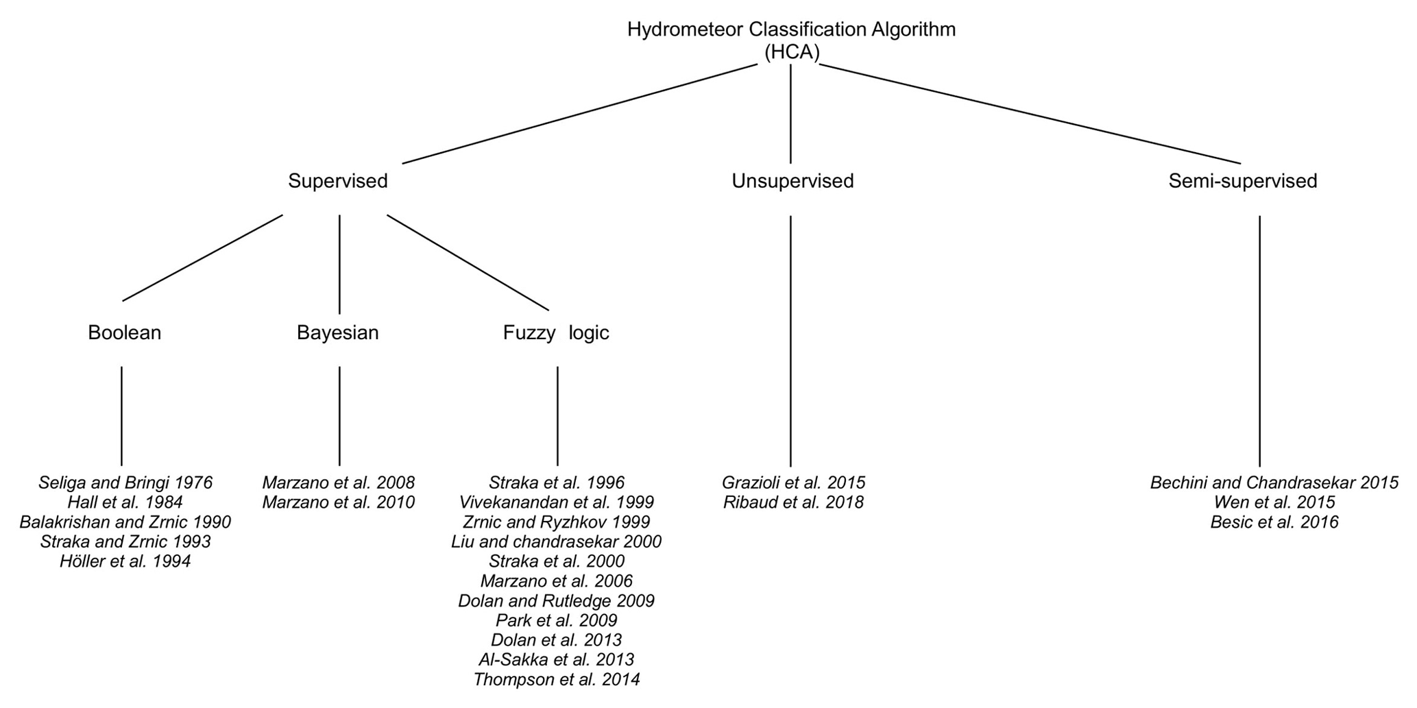
Figure 1Schematic representation of the different hydrometeor classification techniques and their principal associated benchmarks.
Three hydrometeor classification schemes have been developed since the emergence of DPOL radar in the 1980s: (1) supervised, (2) unsupervised, and (3) semi-supervised techniques (Fig. 1).
-
The supervised method constitutes, by far, most of the literature and is subdivided into three different techniques: the Boolean tree method, fuzzy logic, and the Bayesian approach. Here, the supervised technique refers to a priori and arbitrarily identified hydrometeor types from which DPOL radar responses have been derived from either theoretical models or empirical knowledge. Polarimetric observations are then assigned to the most suitable hydrometeor types according to their similarities.
- –
Boolean method. This technique is the easiest way to identify dominant hydrometeor populations and has consequently been the first to be used. The algorithm relies on the beforehand definition of the ranges of DPOL radar-observable values for each hydrometeor type by the user. Then, a simple Boolean decision is applied to retrieve the dominant hydrometeor type (Seliga and Bringi, 1976; Hall et al., 1984; Bringi et al., 1986; Straka and Zrnić, 1993; Höller et al., 1994). This approach, nevertheless, does not take into account the fact that different hydrometeor types can be defined on the same range of values for the same polarimetric radar observable and, therefore, frequently leads to misclassification.
- –
Fuzzy-logic technique (Mendel, 1995). This supervised algorithm type fixed the previous limitation by allowing a smooth transition of DPOL radar-observable ranges for all hydrometeor types. The originality of fuzzy logic is its ability to transform sets of non-linear radar data into scalar outputs referring to different microphysical species. In this regard, each hydrometeor-type distribution is characterized by a membership function coming from either T-matrix simulations (Mishchenko and Travis, 1998) or, less frequently, aircraft in situ measurements. The hydrometeor inference is finally the result of a combination of membership functions and a set of a priori rules defined by the user (Straka, 1996; Vivekanandan et al., 1999; Liu and Chandrasekar, 2000; Marzano et al., 2006; Park et al., 2009; Dolan and Rutledge, 2009; Al-Sakka et al., 2013; Thompson et al., 2014). This method is relatively simple to implement and computationally inexpensive. A few studies, such as the Joint Polarization Experiment (Ryzhkov et al., 2005) for hail detection or even the recent use of a fuzzy-logic algorithm as an operational tool for national weather services (Al-Sakka et al., 2013), have demonstrated the robustness of this hydrometeor classification algorithm type in singular environments.
- –
Bayesian approach. In this case, the hydrometeor identification task is expressed in a probabilistic form based on synthetic data derived from polarimetric radar simulation of different hydrometeor types (with each one being characterized by a centre and a covariance matrix). The final supervised hydrometeor inference is then performed by adapting the maximum a posteriori rule. Another interesting attribute of the Bayesian technique resides in the appealing possibility of retrieving the liquid water content associated with each hydrometeor type (Marzano et al., 2008, 2010).
- –
-
More recently, Grazioli et al. (2015), or even Grazioli et al. (2017), proposed an innovative unsupervised approach to identifying the dominant hydrometeor distribution within precipitation events, where hydrometeor types are retrieved by gathering observable similarities in DPOL radar data. Indeed, the unsupervised technique refers to a set of unlabelled data observations for which the goal is to group them into clusters sharing similar properties based on innate structures of the data (variance, distribution, etc.) and without using a priori knowledge. To achieve this goal, the authors used an agglomerative hierarchical clustering technique together with a spatial constraint on the consistency of the classification (homogeneity). This data-driven approach mainly avoids the numerical-scattering simulations used in fuzzy logic, which are well designed for the liquid phase but questionable for ice-phase microphysics. Finally, interpretation of the clusters (labelling) is done manually.
-
Although initially mentioned by Liu and Chandrasekar (2000), the first complete study based on a semi-supervised approach was done by Bechini and Chandrasekar (2015), recently followed by the works of Wen et al. (2015, 2016) and Besic et al. (2016). This technique combines the advantages of the fuzzy logic and clustering methods. The algorithm initially begins with a fuzzy-logic classification, which is then adjusted by a K-means clustering method that iteratively allows for rectifying the initial membership function of each hydrometeor type according to the observed DPOL radar measurements. In addition, constraints such as temperature limits and/or spatial distribution can be implemented in this self-adapting methodology.
Overall, these hydrometeor classification algorithms (HCAs) still require in situ aircraft validations (especially within convective cores) that are problematic due to their cost and, obviously, the danger of obtaining such measurements. Only a few studies have had the opportunity to use limited aircraft measurements and generally compared a few isolated in situ images with HCA outputs (Aydin et al., 1986; El-Magd et al., 2000; Cazenave et al., 2016; Ribaud et al., 2016b). Another limitation of these studies using methods such as the fuzzy-logic approach is the dependency of their validity, since they are generally both wavelength- and climatically radar-dependent. Although T-matrix simulations for a radar wavelength have been theoretically demonstrated, each final algorithm is then tuned by giving weights to each DPOL radar observable to allow them to fit as closely as possible with local ground observations. Finally, one can also see that the related hydrometeor identification literature is mainly concerned with the midlatitudes. Indeed, the methods were initially developed for S-band radar before being adapted to both C- and X-band radars, and research studies have largely been done in North America, Europe, and Oceania.
The present study aims to develop the first HCA for Brazilian tropical precipitation systems via an X-band dual-polarization radar used in both the GoAmazon2014/5 and ACRIDICON-CHUVA field experiments (Martin et al., 2016, 2017; Wendisch et al., 2016; Machado et al., 2018). Although the area constitutes an intriguing location with both a high amount of rain and complex aerosol–cloud interaction (e.g. Cecchini et al., 2017; Machado et al., 2018), there are almost no references for hydrometeor classification over tropical land, especially for the Amazon region. In this regard, the studies by Dolan et al. (2013) and Cazenave et al. (2016) took place in singular locations (Darwin, Australia, and Niamey, Niger, respectively). These studies used a supervised fuzzy logic approach to retrieve the hydrometeor distribution within precipitation events with a C- and adapted X-band scheme, respectively. As aforementioned, fuzzy-logic algorithms use weights to constrain the final identification. Another issue that might be related to hydrometeor identification tasks is the use of the melting layer as a parameter to detect liquid-ice delineation. However, liquid water above the melting layer within the convective tower of tropical systems is not unusual (Cecchini et al., 2017; Jäkel et al., 2017). For instance, Cecchini et al. (2017) retrieved liquid water at as low as −18 ∘C within polluted tropical convective clouds. Classification using cluster analysis allows the use of natural (non-imposed) classes of ice-water species. For all these reasons, the present paper deals with the first unsupervised clustering method based on X-band DPOL radar measurements in the Brazilian tropical region. Three main questions are addressed in this paper. (1) What is the sensitivity of the clustering algorithm to the different linkage methods, and how can one improve the liquid–solid delineation? (2) What are the hydrometeor classification output characteristics for both wet and dry tropical seasons in Amazonas? (3) What are the microphysical distribution differences within tropical convective and stratiform cloud systems between the wet and dry seasons?
The article is organized as follows: Sect. 2 provides a brief description of the radar dataset, while Sect. 3 presents the AHC method. The sensitivity of the AHC to the linkage methods together with a potential temperature improvement is assessed and discussed in Sect. 4. The hydrometeor identification for Brazilian tropical system events is presented in terms of wet–dry seasons and stratiform–convective regions in Sect. 5, while a discussion of hydrometeor distribution comparisons is presented in Sect. 6.
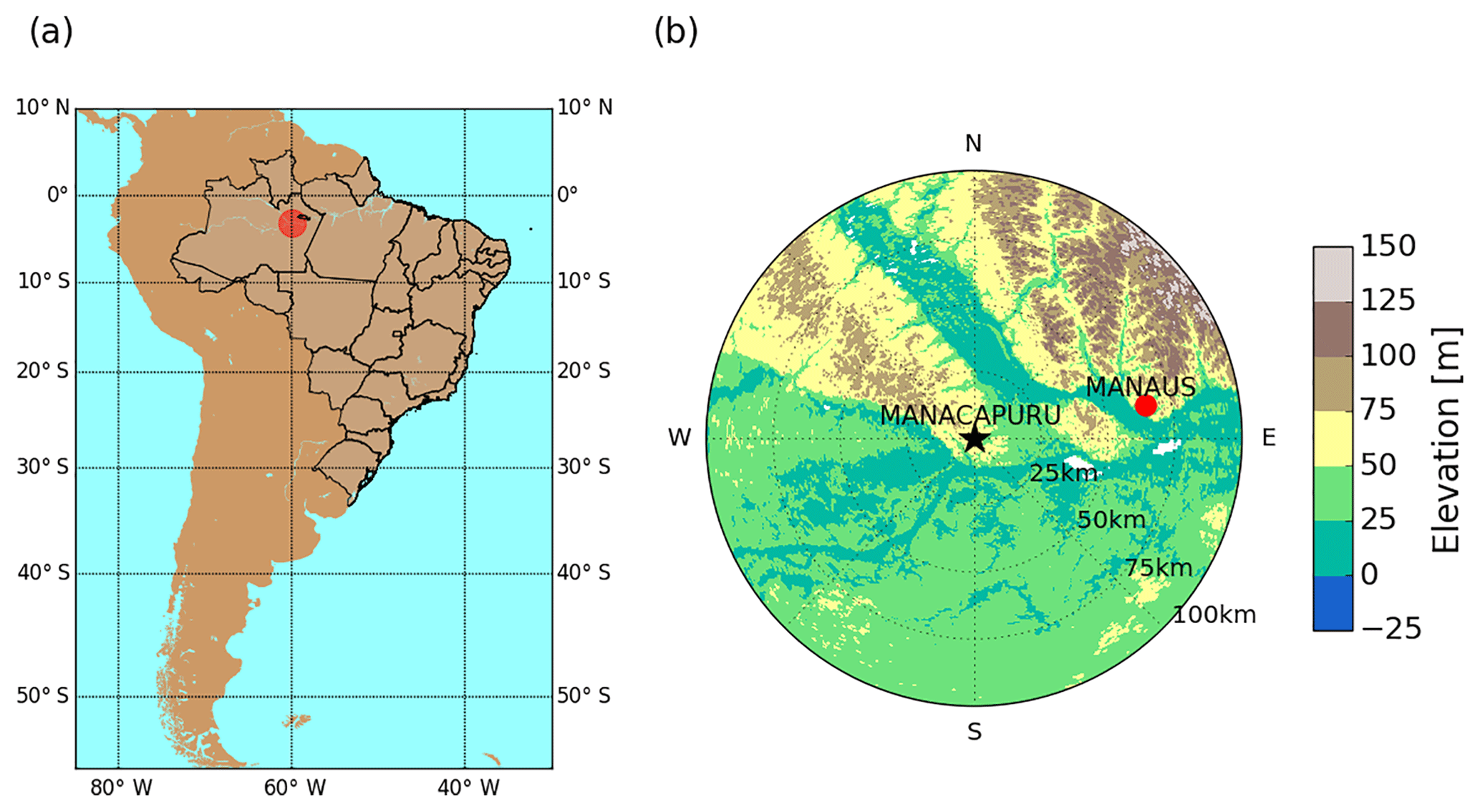
Figure 2(a) Geographical localization of the GoAmazon2014/5 and ACRIDICON-CHUVA experiments. (b) X-band DPOL radar coverage and its associated topography.
The data used in this study are mainly based on DPOL radar data observations collected during both the GoAmazon2014/5 and ACRIDICON-CHUVA experiments that took place around the city of Manaus in the Amazonas state of Brazil (Fig. 2). Both of these research experiments aimed to investigate the complex mechanisms at play within tropical weather through intriguing interactions between human activities and the neighbouring tropical forested region. In this regard, the present study considers the wet and dry seasons as corresponding to the intensive operating periods (IOPs) of the GoAmazon2014/5 field experiment (Martin et al., 2016), which were from 1 February to 31 March 2014 (wet season: 59 days) and 15 August to 12 October 2014 (dry season: 60 days).
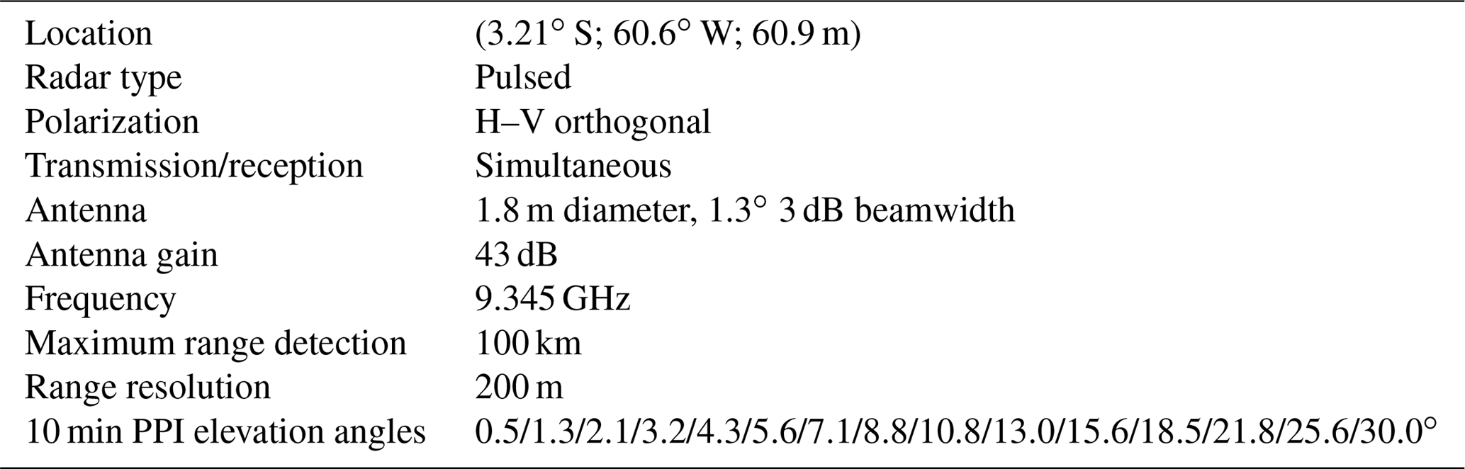
Among all the instruments deployed, a SELEX Gematronik X-band DPOL radar was located in the city of Manacapuru in 2014 to complete the radar coverage from the Manaus Doppler radar, as well as to provide more microphysical details about the South American monsoon meteorological systems (Oliveira et al., 2016). The X-band DPOL radar was operated at 9.345 GHz with a 1.3∘ beam width at −3 dB and in simultaneous transmission and reception (STAR) mode (Schneebeli et al., 2012; and Table 1). The latter characteristic allows the reflectivity to be obtained at horizontal polarization ZH, differential reflectivity ZDR, differential-phase ΦDP, and correlation coefficient ρHV. The scanning strategy was designed to complete an entire volume scan in 10 min by combining 15 different plan position indicators (PPIs) ranging from 0.5 to 30∘, as well as two range height indicators (RHIs) towards randomly different directions.
The raw radar dataset has been processed beforehand to be used for the hydrometeor identification task. In this regard, a four-step process has been applied to the DPOL radar dataset which consists of (i) calibration of ZDR, (ii) identification of meteorological and non-meteorological echoes, (iii) ΦDP filtering and estimation of the derivative specific differential-phase KDP (Hubbert and Bringi, 1995), and (iv) attenuation correction applied to both ZH and ZDR based on the ZPHI method proposed by Testud et al. (2000). The calibration of ZDR has been adjusted by using vertically pointing scans for cases with no rain attenuation (drizzle/light rain). This method allows the ZDR offset to be temporally calculated since 0 dB is expected. The offset has been then removed in subsequent ZDR measurements. A second analysis of ZDR was occasionally realized by checking ZDR values within a stratiform light-rain medium and characterized by ZH values between 20 and 22 dBZ. The expected ZDR value was 0.2 dB as shown by Illingworth and Blackman (2002) or Segond et al. (2007). Note that the dataset has also been restricted to precipitation events wherein the radome of the X-band DPOL radar was dry in order to remove any additional attenuation (Bechini et al., 2010). In addition to these considerations, a signal-to-noise ratio of SNR dB as well as a reduced radar coverage ranging from 5 to 60 km, have been considered for this study to mitigate potential remaining errors. The last processing step relies on the separation of stratiform and convective radar echoes. The methodology used in the present paper is the same as that used by Steiner et al. (1995) and has been applied from a horizontal reflectivity field at a constant altitude plan position indicator (CAPPI) generated at 3 km height (T>0 ∘C).
The present study also deals with external temperature information coming from soundings launched near the X-band radar (downwind of Manaus) at 00:00, 06:00, 12:00, 15:00, and 18:00 UTC. The sounding with the closest time to the radar measurements has been considered to derive the temperature profile associated with both PPIs and RHIs.
The present hydrometeor classification algorithm is an unsupervised AHC method that aims to partition a set of n observations into N different clusters. This technique works as an iterative bottom-up method where each observation starts in its own cluster and pairs of clusters are aggregated step by step until there is one final cluster, which comprises the entire dataset. Each cluster is composed of a group of observations sharing more similar characteristics than the observations belonging to the other clusters. Here, there is no a priori information concerning the shape and size of each cluster or the final optimized number of clusters. A posteriori analysis is then performed through the final iterations to retrieve the optimal clustering partition and respective labels.
Since the associated background already exists, the reader is especially referred to Ward (1963) and Jain et al. (2000) for detailed mathematical reviews of the technique. Additionally, the present clustering framework is mainly based on the methodology developed by Grazioli et al. (2015, Sect. 4 and Fig. 2), hereafter referred to as GR15, and only relevant and important information will be addressed hereafter to avoid being redundant. The main steps of the present AHC can be summarized as follows:
-
Vectorized objects of radar observations are defined for each valid radar resolution volume as
where Δz is the difference between the radar resolution height and the altitude of the isotherm at 0 ∘C, deduced from sounding balloons.
-
Since scales of radar polarimetric variables differ by orders of magnitude, data normalization is applied to concatenate all the observations into a [0;1] common space. The first four components of each object are based on the minimum–maximum boundaries rule. The temperature information is redistributed by applying a soft sigmoid transformation that allows a value of zero (one) to be set for altitudes below (over) the bright band. Here, the thickness of the bright band over the whole GoAmazon2014/5 – ACRIDICON-CHUVA database has been manually estimated and set up to spread over a layer of ±700 m. To obtain the maximum degrees of freedom in the initial dataset coming from the DPOL radar measurements, here, the influence of the temperature information is mitigated by distributing its values into a [0;0.5] range space.
-
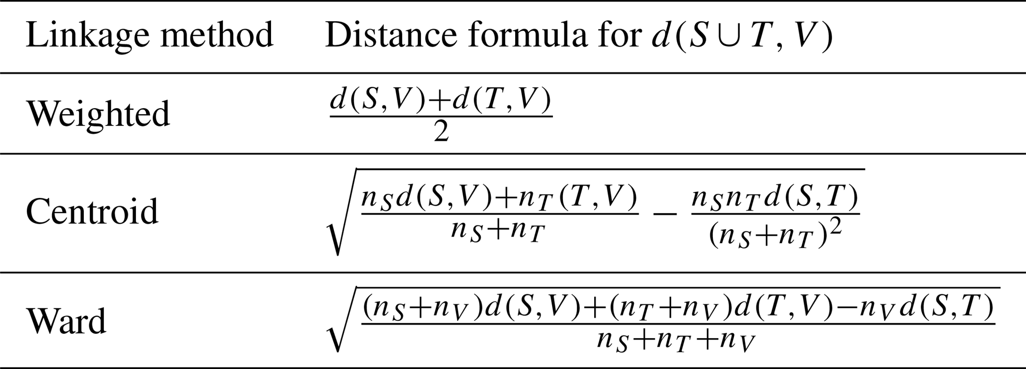
Although the radar data are now suitable for clustering, the choice of two criteria still remains. At each iteration of the AHC method, similarities and dissimilarities must be evaluated to determine which clusters merge. In this regard, the Euclidean metric is considered to calculate the distance between different single objects. The generalization of this distance metric to an ensemble of objects is called the merging linkage rule. Various methods exist to evaluate interdissimilarities such as single (nearest neighbour), complete (farthest neighbour), averaged, weighted, centroid, or even Ward (variance minimization) linkages (see Müllner, 2011). Herein, we consider the weighted, centroid, and Ward linkage rules (see Sect. 4.1).
-
Running a clustering method over the whole dataset is computationally very expensive. To tackle this problem, a subset of approximately 25 000 initial observations is randomly chosen through the whole precipitation events database. The clustering method is initially applied to the subset and then extended to the whole dataset by using the nearest-cluster rule at each iteration.
-
One of the major novelties proposed by GR15 relies on the implementation of a spatial constraint that aims to check the homogeneity of the clustering distribution at each iteration. More precisely, one assumes that a smooth, horizontal transition exists between the resulting hydrometeor field outputs. Therefore, a spatial smoothness index is calculated at the end of each iteration step and individual object by checking the four closest geographical radar gates. In the very same way as that used in GR15, results are summarized into a confusion matrix, from which several spatial indexes can be extracted to analyse the individual and global spatial smoothness of a partition.
-
The merging of two clusters is realized by identifying the cluster which presents the lowest spatial similarities among all clusters. Objects belonging to this spatially poor cluster are then constrained to be redistributed through the other existing clusters according to the linkage method chosen. This final step allows a reduction of the total number of clusters by one.
-
If the iteration process does not reach a single and unique cluster, the iteration loop then restarts at the initial PPI classification and goes through the evaluation of spatial homogeneity.
-
Finally, an analysis of the variance explained has been implemented to evaluate the consistency of the clustering classification outputs. This quality metric allows a definition of the theoretically appropriate number of clusters by analysing the ratio between the internal and external variance of each cluster at each step of the iteration. The main idea here is to find the optimal cluster distribution beyond which considering one more cluster is not meaningful.
Table 2Distance formulas for the weighted, centroid, and Ward linkage rules. Here, S and T are two clusters joined into a new cluster, whereas V is any another cluster. nS, nT, and nV are the number of objects contained in the clusters S, T, and V.
4.1 Linkage rule sensitivity
According to the set-up described in Sect. 3, different linkage rules have been tested through the special wet-season observation period (February to March) of 2014. To perform this sensitivity test, three different linkage rules have been considered here: (i) weighted, (ii) centroid, and (iii) Ward (see Table 2 for their respective formulas). Since the clustering method randomly picks observations within the whole wet-season period, a set of numerous runs for each linkage method have been performed to extract, as much as possible, the most representative behaviour of each one. The general common set-up is composed of a subset of 25 000 observations randomly picked through more than 50 precipitation days. The temperature information is based on radiosounding observations and is dispatched in a [0;0.5] interval to place twice as much importance on the initial DPOL radar observations. The number of clusters reached in the first step of the AHC method is set at 50 (far enough from the final partition and not too computationally expensive). Finally, the clustering method has been conducted separately on stratiform and convective regions.
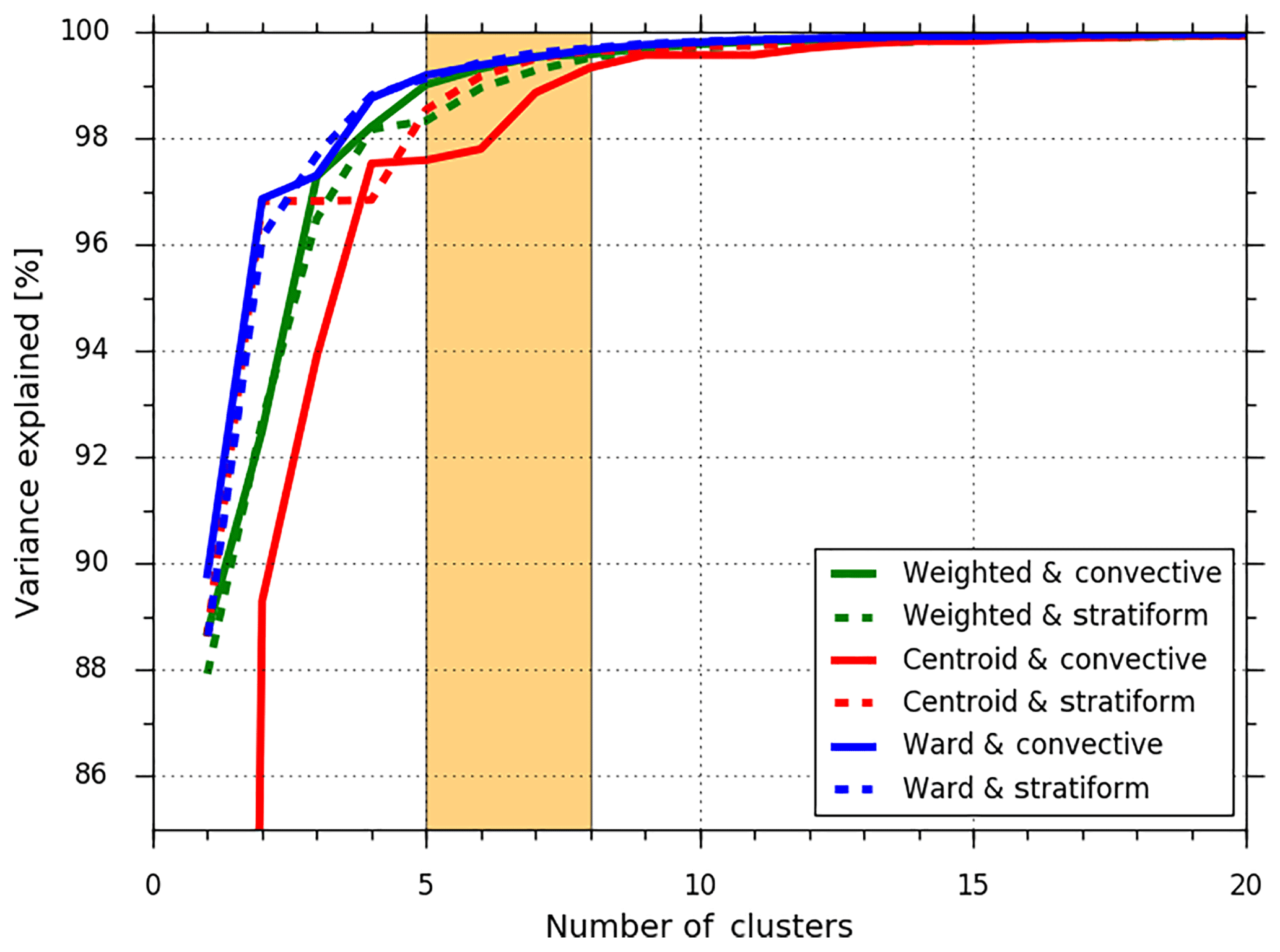
Figure 3Evolution of the variance explained for different clustering linkage rules. Each linkage method is subdivided in terms of stratiform (dashed line) and convective (solid line) regions. The orange vertical span highlights the interval potentially associated with the optimal number of clusters.
In this respect, Fig. 3 presents the evolution of the variance explained (the ratio between the internal and external variance) for the three different linkage rules as a function of the number of clusters considered, together with their associated precipitation regimes (stratiform or convective). Overall, the three methods exhibit an “elbow” curvature with an optimal number of clusters ranging from approximately 5 to 8 (orange background on Fig. 3). One can see that from 2 to 5 clusters, the explained variances sharply increases, meaning that each added cluster within this interval contributes significantly to retrieving the most adequate cluster partition. From 5 to 8 clusters, the increase starts to slow down, indicating that considering a greater number of clusters is not meaningful. In this regard, the best compromise seems to be the weighted and/or Ward linkage method for both stratiform and convective regions. Indeed, these methods have the highest scores, with approximately 99 % reached within the 5–8 cluster interval.
Due to the inherent complexity of representing all the potential combinations, manual analysis and selection have been performed beforehand to find the optimal number of clusters between the stratiform and convective regions. The results from this partitioning are presented through one stratiform and one convective RHI (Figs. 4 and 5).
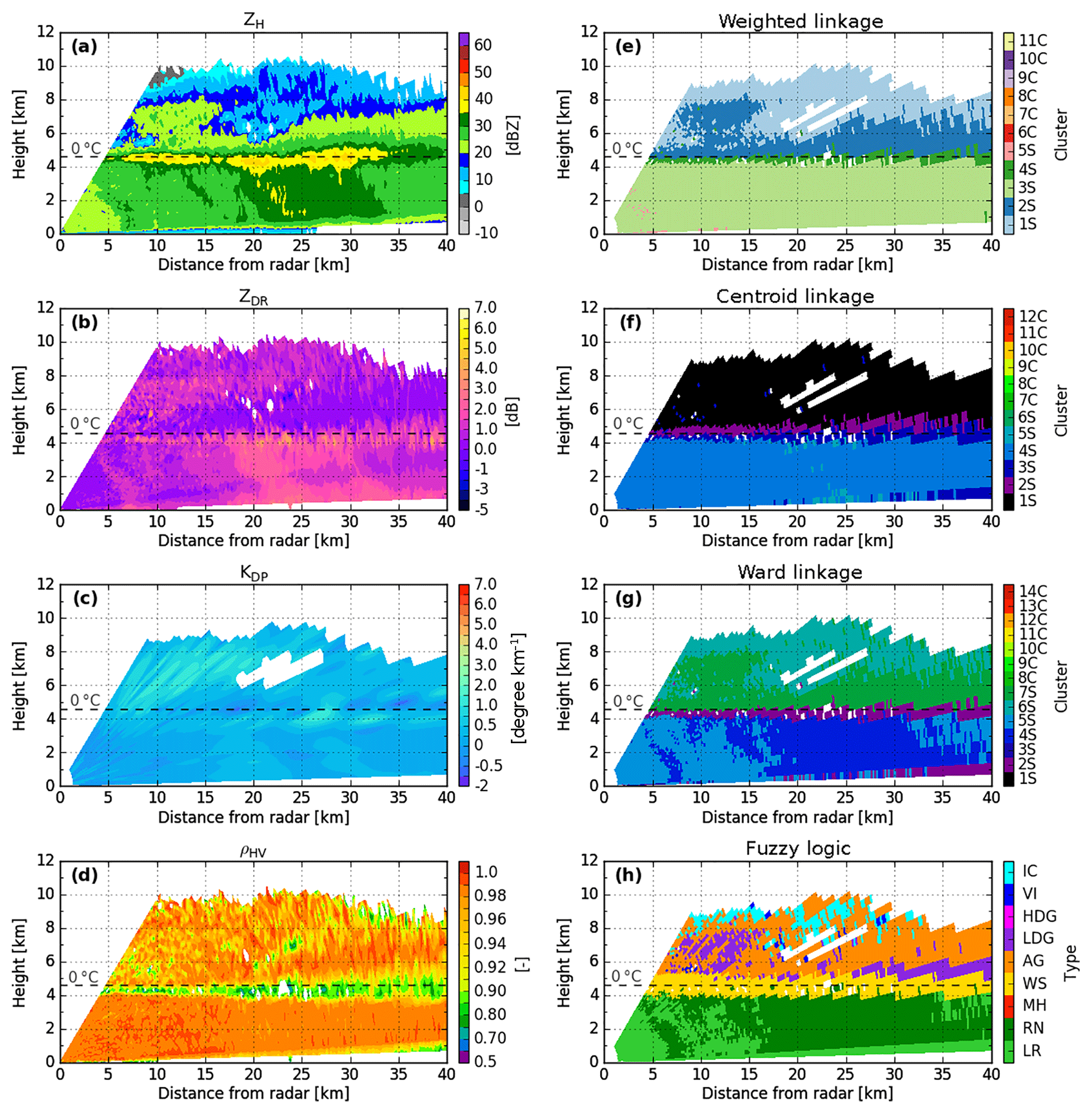
Figure 4X-band DPOL radar observables and the corresponding retrieved hydrometeor classification outputs at 12:07 UTC on 21 February 2014, along the azimuth 290∘. DPOL radar observables are shown in (a) ZH, (b) ZDR, (c) KDP, and (d) pHV. Comparisons of retrieved hydrometeors for clustering outputs based on (e) weighted, (f) centroid, and (g) Ward linkage rules and (h) fuzzy-logic scheme outputs. In (e)–(g), each number corresponds to a different cluster. S stands for stratiform regimes, whereas C is for convective regimes.
In addition, fuzzy-logic information has been implemented to make comparisons with cluster outputs. The fuzzy-logic scheme is mainly based on the X-band algorithm of Dolan and Rutledge (2009), hereafter referred to as DR09, and has been slightly enriched for the wet-snow and melting-hail hydrometeor types by Besic et al. (2016) through scattering simulations and a temperature membership function (Besic et al., 2016, Appendix A). Finally, the adapted fuzzy-logic allows discrimination between nine hydrometeor types: light rain (LR), rain (RN), melting hail (MH), wet snow (WS), aggregates (AG), low-density graupel (LDG), high-density graupel (HDG), vertically aligned ice (VI), and ice crystals (IC).
Figure 4 shows a stratiform system exhibiting a well-defined bright-band signature from polarimetric observations that occurred on the shores of the Amazon River on 21 February 2014. Overall, the centroid linkage method does not reproduce the event well, and the final representation is microphysically poor (Fig. 4f). Indeed, this linkage rule simply divides the cloud into three homogeneous regions (T>0 ∘C, T∼0 ∘C, and T<0 ∘C). Additionally, the centroid linkage fails to identify a clear bright-band region (Fig. 4f, clusters 2S and 3S). On the other hand, the weighted and Ward linkage methods are very close to the fuzzy-logic output descriptions (Fig. 4e, g, h). They both exhibit two kinds of rain, and a bright-band region sits below what appears to be an aggregate–ice crystals mixture. The main discrepancy here concerns the representation of the rain structure. The Ward linkage rule retrieves two more distinct liquid species (as does fuzzy logic), whereas the weighted linkage method exhibits a smoother rainy region.
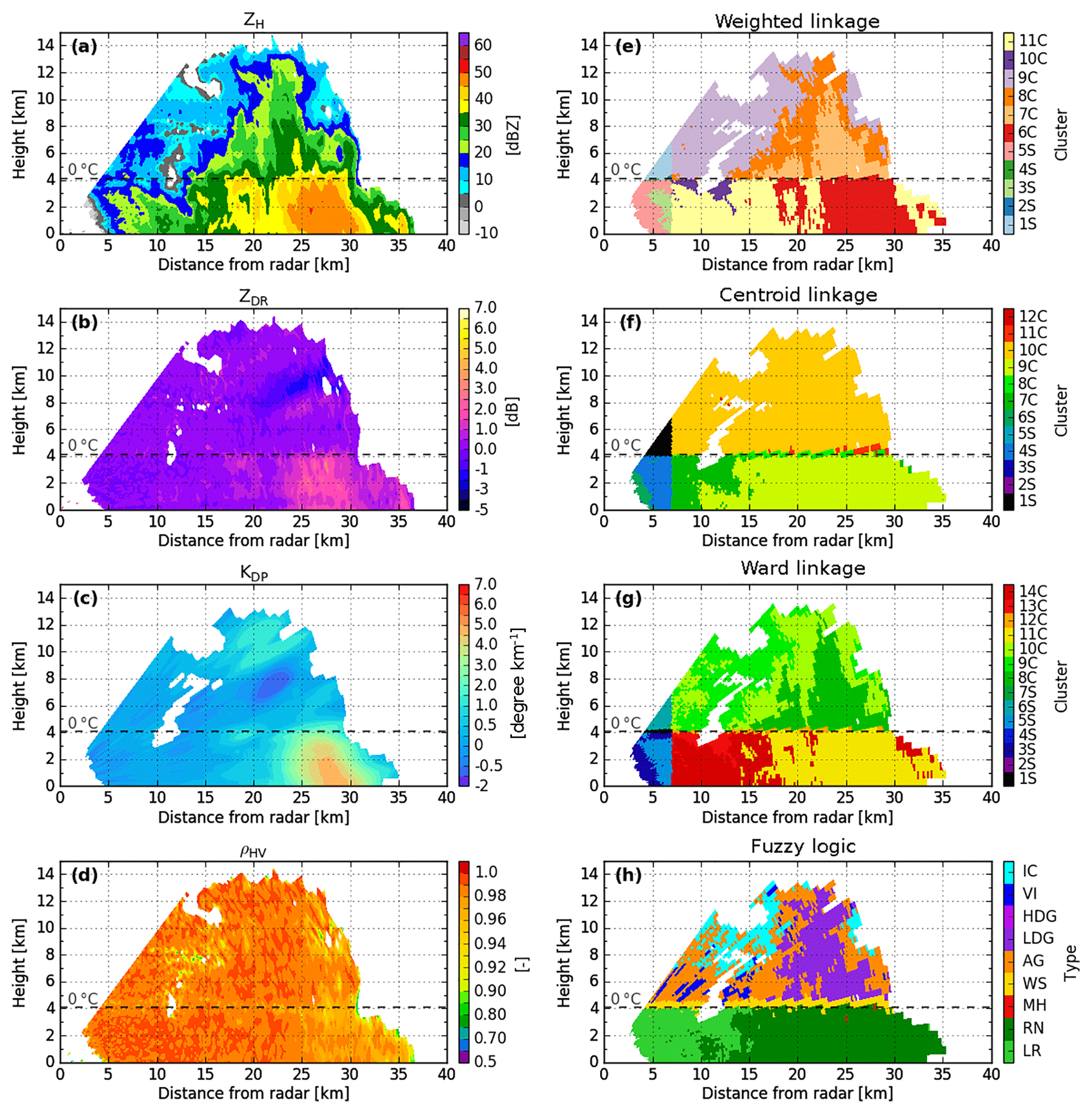
Figure 5 presents a decaying convective cell that occurred on 2 February 2014 at 13:57 UTC (0–7 km from the radar: stratiform region, 7–40 km from the radar: convective region). As is the case for the stratiform RHI in Fig. 4, the centroid linkage rule fails to retrieve a detailed microphysical structure and only presents very homogeneous liquid and solid regions. Once again, both the weighted and the Ward linkage rules stand out and display a more realistic hydrometeor description of the convective cloud in comparison to the DPOL radar observations and the fuzzy-logic outputs (Fig. 5a–e, g, h). Although they both present three clusters for T>0 ∘C, the weighted linkage rule puts more emphasis on the convective region located ∼20–30 km from the radar than does the Ward linkage (Fig. 5e, cluster 6C vs. Fig. 5g, cluster 11C). The representation of the solid region (T<0 ∘C) is almost the same, except for in the aggregate region (Fig. 5h), which seems to be smaller for the weighted linkage rule (Fig. 5e cluster 8C) than for the Ward method (Fig. 5g cluster 10C). Another discrepancy between the weighted and Ward linkages concerns the layer around the isotherm at 0 ∘C. Although Fig. 5 does not exhibit any bright-band region, the Ward linkage rule does exhibit one due to the temperature input (Fig. 5g cluster 12C), whereas the weighted rule does not. The bright-band region is known to be well defined for stratiform regimes but quasi-undetectable (if detectable at all) for convective areas (Leary and Houze Jr., 1979; Smyth and Illingworth, 1998; Matrosov et al., 2007). Throughout the present paper, one will thus consider only a bright-band cluster for the stratiform regions, whereas convective areas will be lacking one.
Overall, Figs. 3, 4, and 5 have shown that the centroid linkage method is inappropriate for the present task, whereas both weighted and Ward linkage rules are able to retrieve a detailed microphysical structure within the sample cloud. Based on the present description and our personal analysis over the whole dataset, we chose to keep working with the weighted linkage rule throughout the remainder of the paper.
4.2 Potential improvement around isotherm 0 ∘C
High amounts of liquid water a few kilometres above the isotherm at 0 ∘C are not rare within the core of convective tropical cells. Sometimes, super-cooled liquid drops can be maintained and even moved upward within the melting layer, thus occasionally giving distinctive column-shaped polarimetric signatures for ZDR∕KDP (e.g. Kumjian and Ryzhkov, 2008). A simple liquid–solid delineation based only on the temperature profile is therefore unsuitable.
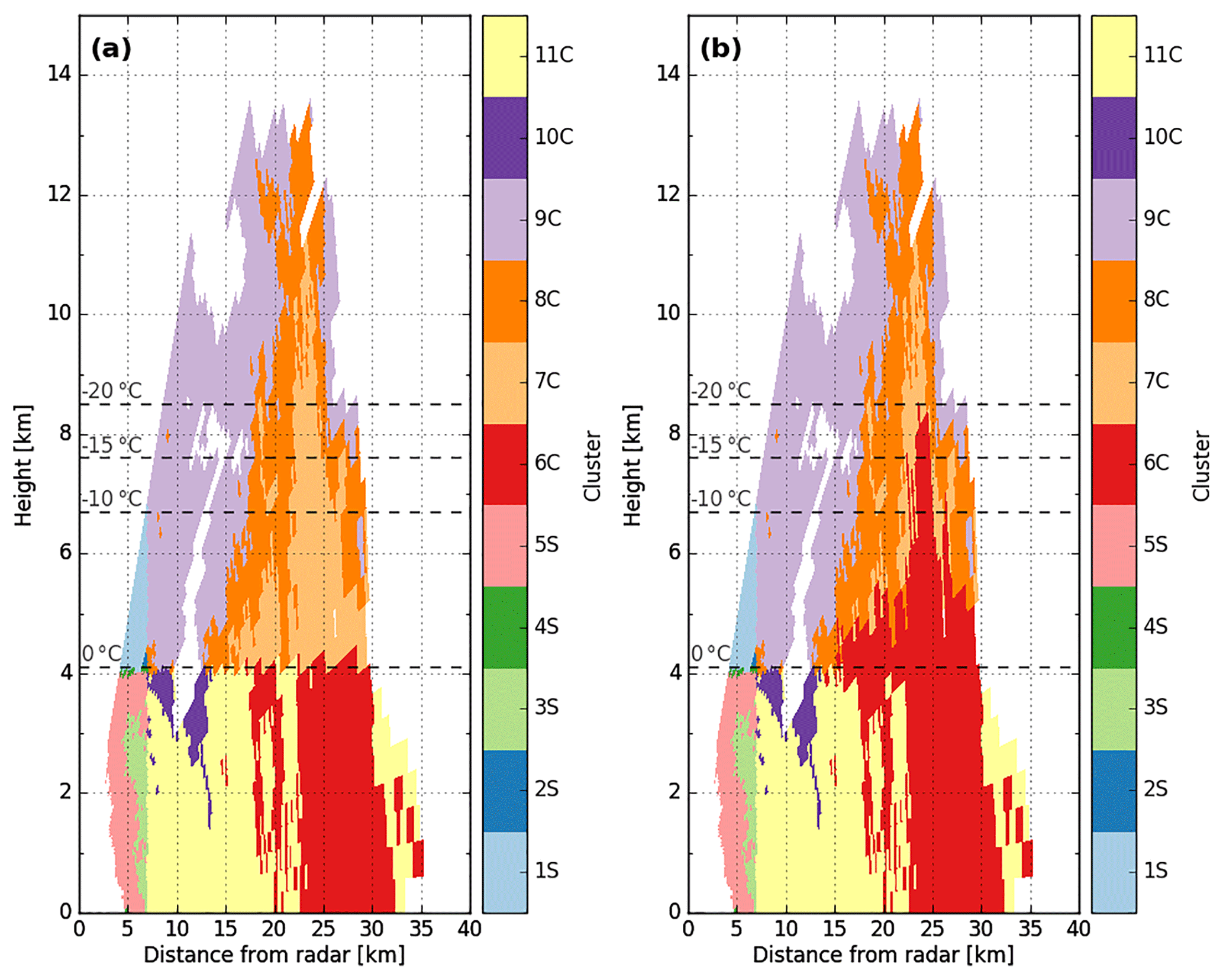
Figure 6Clustering hydrometeor classification retrieved from the X-band radar at 12:07 UTC on 21 February 2014, along the azimuth 290∘. (a) With temperature constraint, (b) without temperature constraint.
Figure 6 presents an adaptive solution for tackling this issue based on the clustering outputs of the weighted linkage rule. The solution proposed here relies on a posteriori analysis of the clustering outputs associated with the convective regions. First, one proceeds to identify the convective core under the isotherm at 0 ∘C (here, cluster 6C). Then, all radar observations within the solid region are assigned by calculating their distance from the 6C cluster centroid without applying any temperature constraint (objects are thus defined only by the first four radar components). If the distance is smaller than D<0.25 and there is no discontinuity throughout the liquid–solid delineation, then the solid identification is switched to liquid (cluster 6C). Note that the distance D has been empirically chosen for the present radar observations and could consequently be adjusted by exploring more convective days. Overall, with this simple hypothesis, one can see the potential of a such method (Fig. 6b). The liquid cluster can thus reach 8 km in the core of the convection at 25 km from the radar, which matches well with the convective tower (>35 dBZ) visible in Fig. 5a. Around this convective core, the enhancement allows raindrops to be raised by about 1 km upward in the 0 ∘C isotherm, restraining cluster 6C at ∼5 km. In comparison to a simple binary delineation such as that used for the fuzzy-logic outputs (Fig. 6a), the focus on radar observables in a second phase is then promising.
This section aims to interpret and label each cluster retrieved through both the wet and dry seasons over the Manaus region by using the AHC method set-up described in Sect. 3. As the use of classification allowing liquid water above the melting layer of convective towers needs further validation, a standard classification is used to classify and analyse the wet and dry hydrometeors using the temperature parameter.
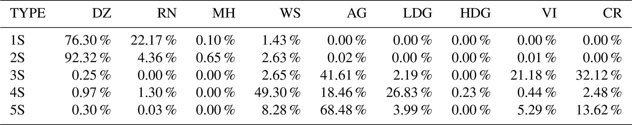
Table 3Confusion matrix comparing the clustering outputs from the stratiform region of the wet season and hydrometeor species retrieved from the adapted fuzzy logic.
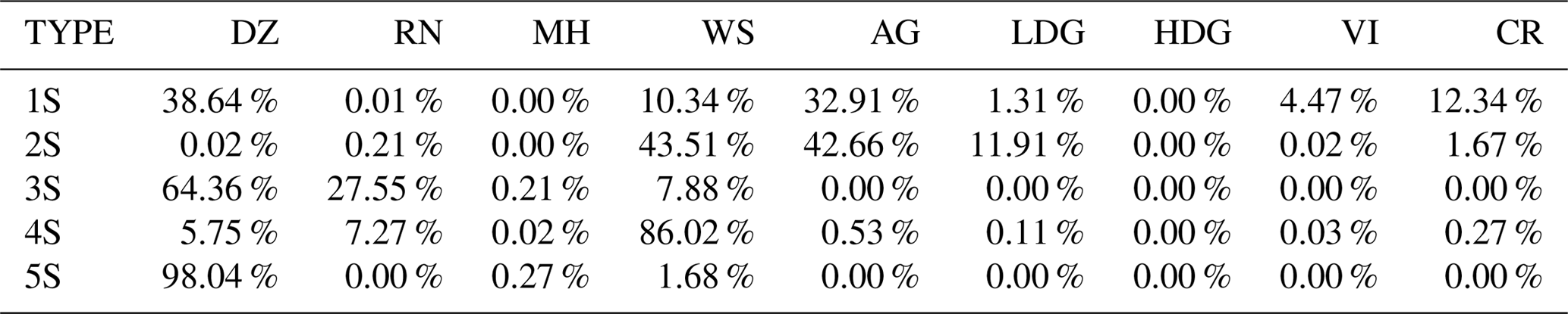
Table 4Same as Table 3, but for the convective region of the wet season.
5.1 Wet-season clustering outputs
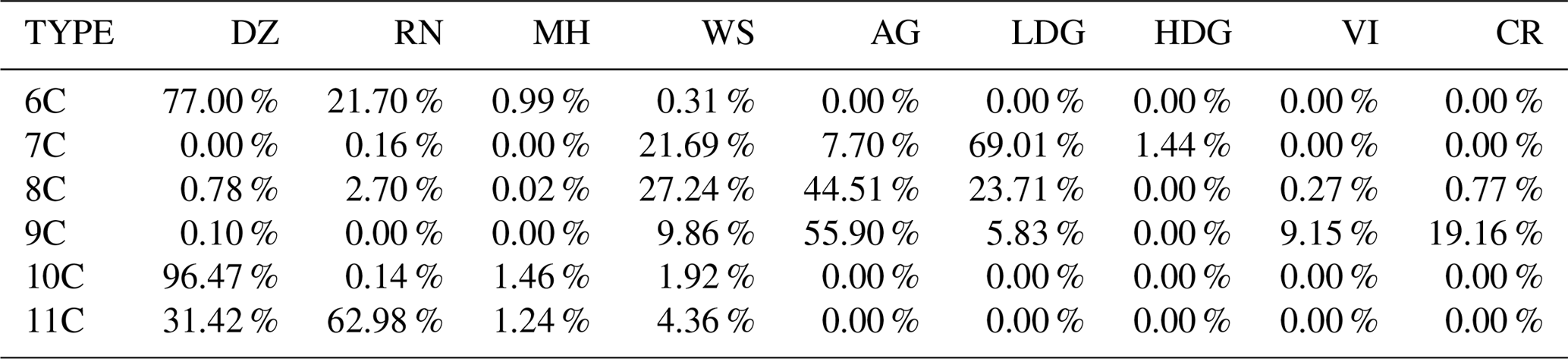
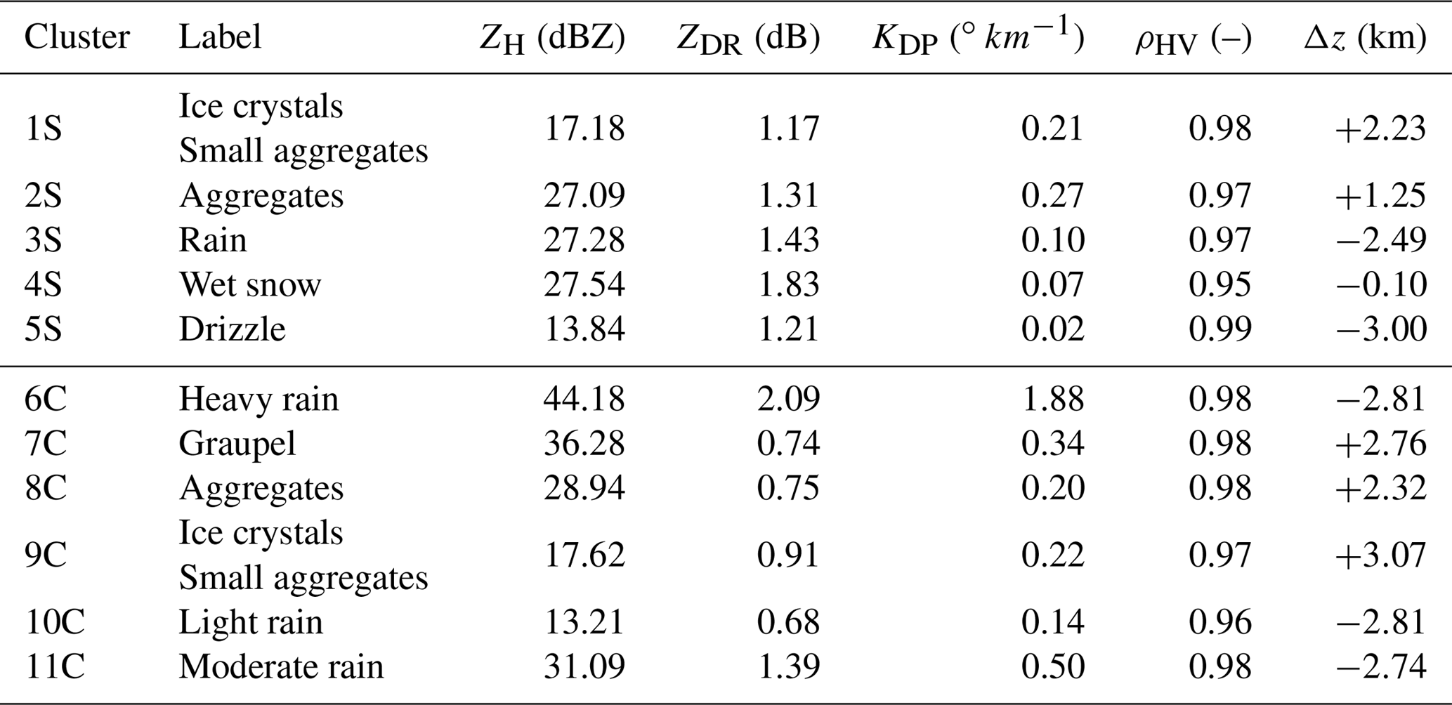
The distributions of ZH, ZDR, KDP, ρHV, and Δz for each cluster from the stratiform and convective clouds of the wet season together with their probability densities are presented in the violin plot in Figs. 7 and 8. The contingency table between the stratiform (convective) clustering outputs and the nine microphysical species retrieved by the DR09 adapted fuzzy-logic algorithm is shown in Table 3 (Table 4). The complete wet-season cluster centroids are given in Appendix Table A1.
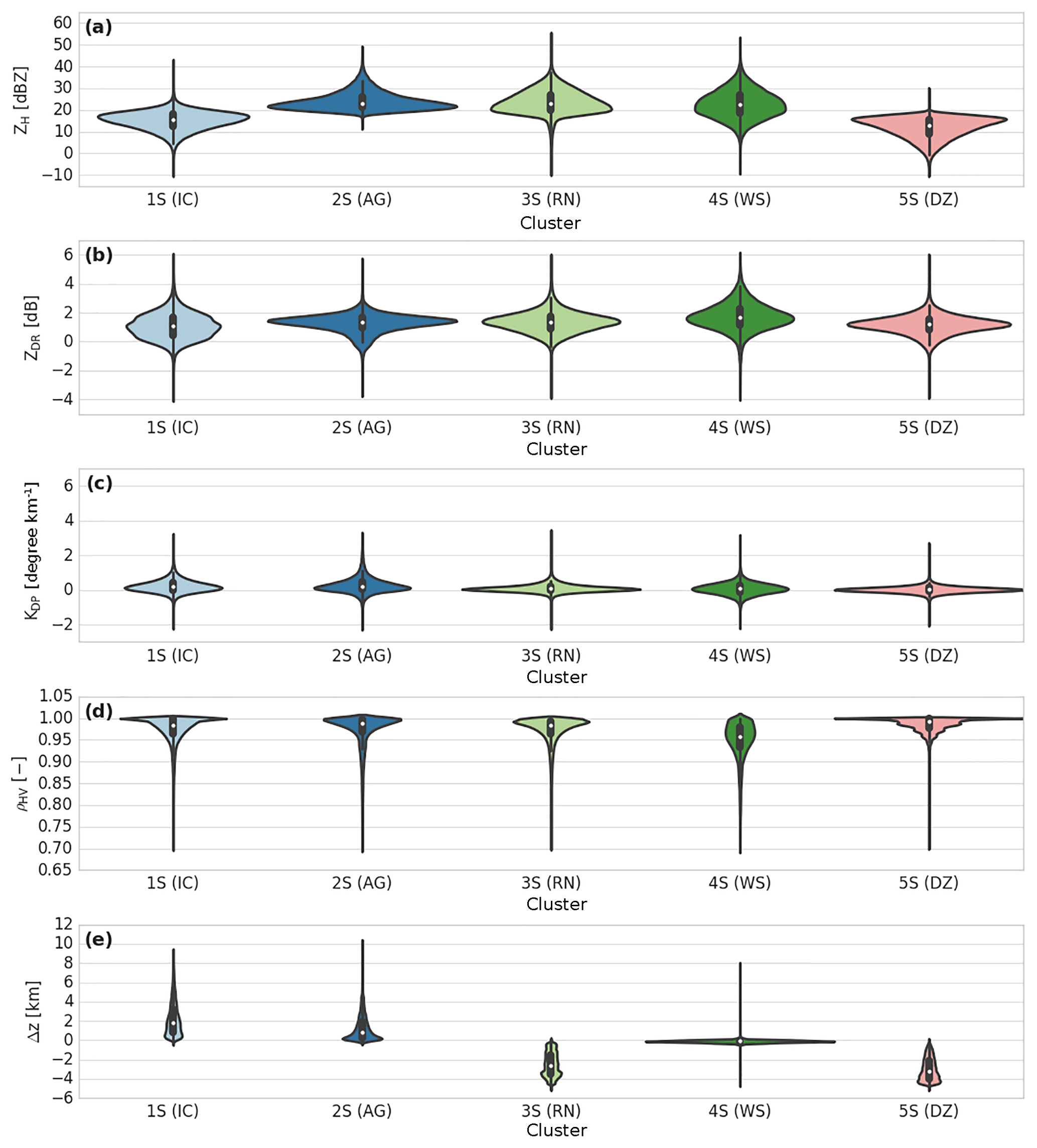
Figure 7Violin plot of cluster outputs retrieved for the stratiform regime of the wet season (DZ is drizzle, RN is rain, WS is wet snow, AG is aggregates, and IC is ice crystals). The thick black bar in the centre represents the interquartile range, and the thin black line extended from it represents the 95 % confidence intervals, while the white dot is the median.
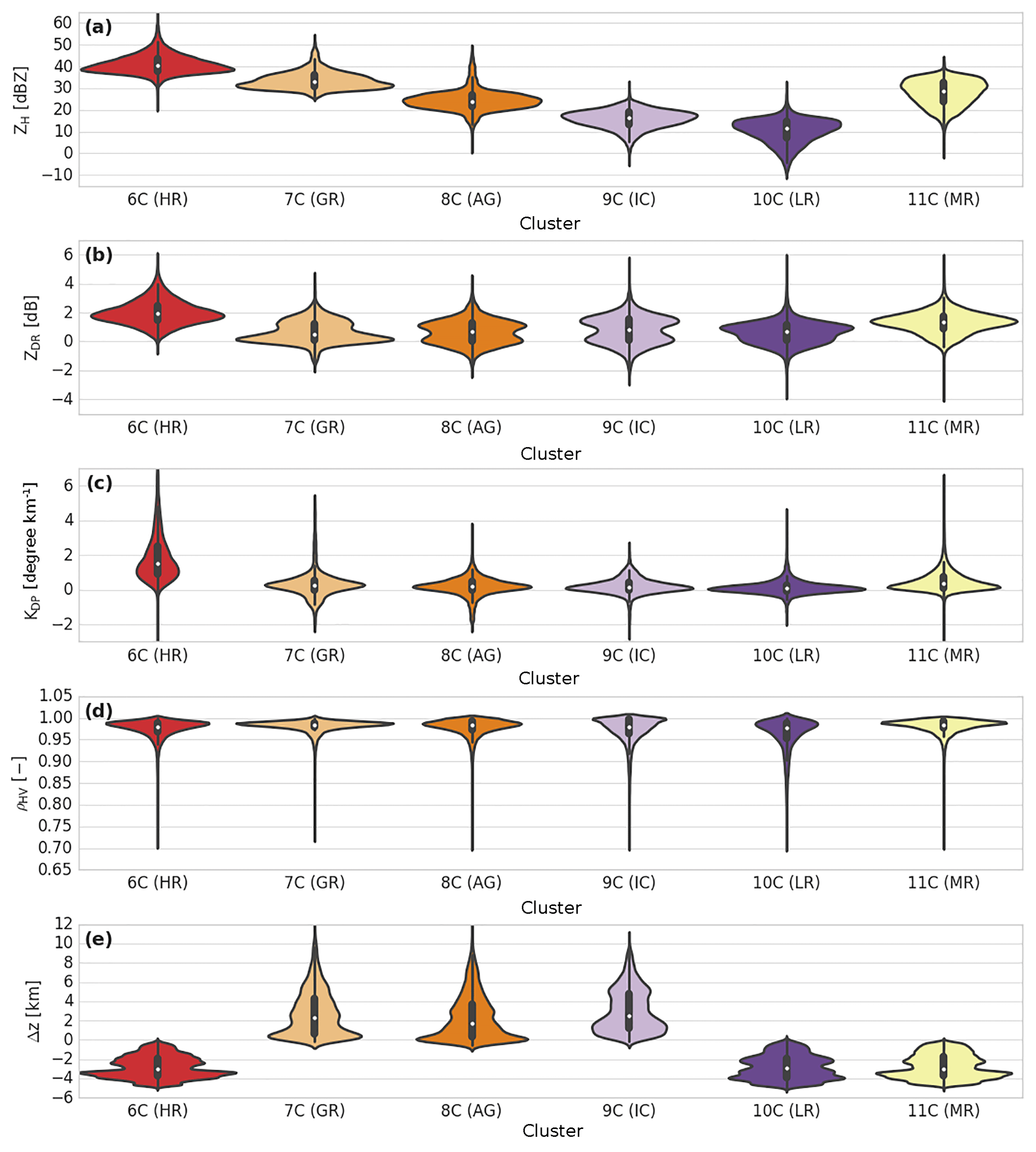
Figure 8Same as Fig. 7, but for the convective regime of the wet season (LR is light rain, MR is moderate rain, HR is heavy rain, GR is graupel, AG is aggregates, and IC is ice crystals).
5.1.1 Stratiform region
Cluster 1S is only defined for negative temperatures and is associated with high ρHV and low ZH, ZDR, and KDP values (Figs. 4e and 7). One can see from contingency Table 3 that the cluster 1S repartition is mostly associated with aggregates (∼33 %) and ice crystals (∼12 %) for high altitudes. Although the horizontal and differential reflectivity values are slightly higher than those for the DR09 T-matrix microphysical outputs and polarimetric characteristics retrieved by GR15, one can make the assumption that the cluster 1S behaviour stands for ice crystals. On the other hand, cluster 2S is closer to the DR09 T-matrix aggregates of microphysical features. This cluster is characterized by a mean horizontal (differential) reflectivity of ∼27 dBZ (∼1.3 dB), a low specific differential phase (∼0.27 ), and a high coefficient of correlation (0.97). Overall, the polarimetric signatures of cluster 2S are mostly divided into the associated wet and dry snow (aggregates) from the microphysical categories of fuzzy logic (Table 3). Figure 4e allows discrimination between these categories, and one can consider that here cluster 2S is associated with aggregates. Once again, its polarimetric signatures are slightly higher than the DR09 T-matrix values or even the GR15 aggregate clustering output. One explication behind these distributions being slightly shifted to higher values can be the relative humidity, which is higher in the tropics than at higher latitudes. The growth of ice crystals/aggregates by vapour diffusion within this cloud region (Houze, 1997) may lead to bigger solid particles (higher ZH and ZDR values).
The bright-band region is well represented here by cluster 4S. Indeed, its global distribution spreads only at the altitude of the isotherm at 0 ∘C and exhibits high ZH and ZDR values, as well as low KDP and ρHV values. Finally, clusters 3S and 5S present rain characteristics, since more than 90 % of these clusters are in agreement with the drizzle and rain fuzzy-logic types from DR09. Although the two clusters have the same behaviour, cluster 3S is characterized by polarimetric signatures higher than those in cluster 5S, except for the coefficient of correlation (0.97 vs. 0.99). In this regard, one can consider that cluster 3S represents the rain microphysical species, whereas cluster 5S is related to drizzle characteristics.
5.1.2 Convective region
Overall, one can see from Figs. 5 and 8 that the convective regions of the wet season are composed of three types of hydrometeors for both positive (clusters 6C, 10C, and11C) and negative temperatures (clusters 7C, 8C, and 9C).
Hail precipitation in the Amazonas region is rare, and as expected, no clusters represent melting hail characteristics, as in Ryzhkov et al. (2013) or Besic et al. (2016) (Table 4). Therefore, clusters 6C, 10C, and 11C can be associated with three distinct rainfall precipitation regimes. In this regard, cluster 10C presents the same light-rain characteristics as both DR09 and GR15. The cluster is characterized by ZH (ZDR) values approximately 13 dBZ (0.68 dB), and a KDP (0.14 ) that is in high agreement with the drizzle hydrometeor type from the adapted fuzzy logic (∼97 %, Table 4). According to this description, one can attribute cluster 11C to the light-rain precipitation type. The two remaining liquid clusters are associated with moderate and heavy rainfall types with almost the same polarimetric signatures as those given in GR15. Indeed, cluster 6C presents higher ZH (44 vs. 31 dBZ), ZDR (2.1 vs. 1.4 dB), and KDP (1.9 vs. 0.8 ) mean values than those for cluster 11C. In this regard, one can link cluster 6C to heavy rainfall and cluster 11C to moderate rainfall.
Concerning negative temperatures, cluster 9C stands out by being spread at the highest altitudes (Fig. 8e). This cluster is defined by low ZH, ZDR, and KDP values together with a moderate ρHV (∼0.97). One can note that cluster 9C is close to the ice crystals and small aggregates retrieved by GR15 and is also the only cluster related to the T-matrix ice crystals species from DR09 (Table 4). Within the decaying convective cell presented in Fig. 5, one can observe that cluster 7C is associated with the low-density graupel characteristics proposed by DR09 and exhibits ZH (ZDR) values approximately 36 dBZ (0.8 dB). In addition, cluster 7C is mainly classified (∼69 %) as low-density graupel (Table 4). Finally, the last cluster, 8C, is surrounded by ice crystals and presents polarimetric signatures lower than those for cluster 7C. Although it is defined by higher values than those given by DR09 and GR15, one can associate cluster 8C with the aggregate microphysical species. Indeed, contingency Table 4 shows that 45 % of the cluster 8C points are in agreement with this hydrometeor type.
5.2 Dry-season clustering outputs
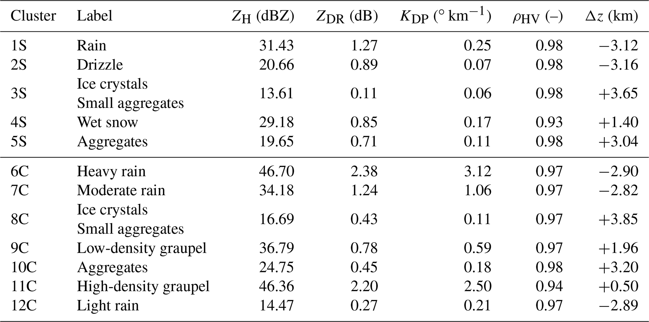
As for the previous section, the clustering outputs retrieved by the AHC method and the weighted linkage rule are identified and associated with their corresponding microphysical species through the dry tropical season. The corresponding cluster centroids are detailed in Appendix Table A2.
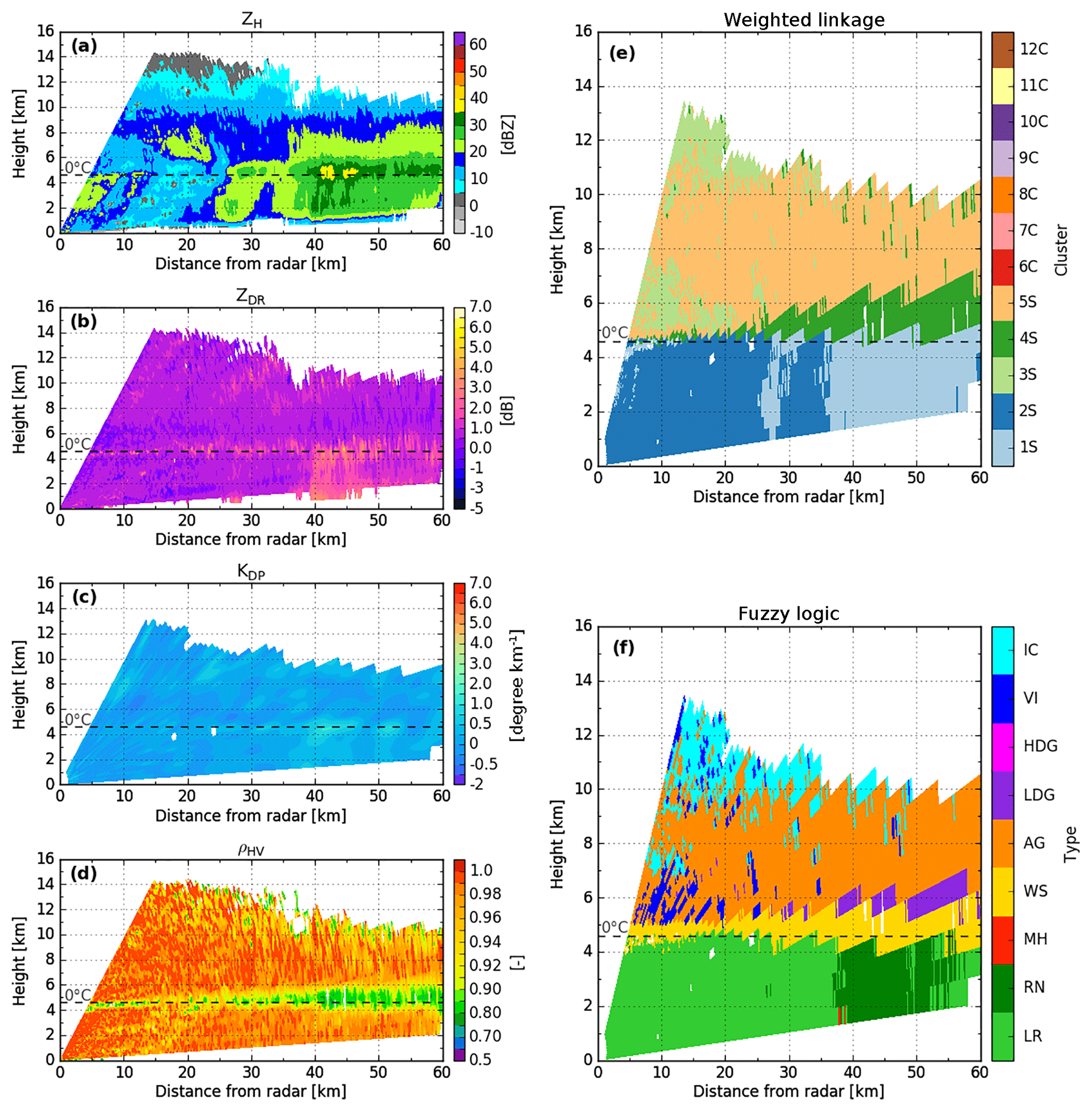
Figure 9X-band DPOL radar observables and the corresponding retrieved hydrometeor classification outputs at 21:26 UTC on 8 September 2014, along the azimuth 200∘. DPOL radar observables are shown in (a) ZH, (b) ZDR, (c) KDP, and (d) pHV. Comparisons of retrieved hydrometeors for clustering outputs based on (e) weighted linkage rules and (f) the fuzzy-logic scheme. In (e)–(f), each number corresponds to a different cluster. S stands for the stratiform region, whereas C is for the convective region.
5.2.1 Stratiform region
Figure 9 shows the clustering classification outputs extracted from an RHI presenting a melting layer region within a stratiform event that occurred on 8 September 2014 in the region of Manaus. Overall, the clustering outputs are close to the hydrometeor distribution retrieved by the adapted DR09 fuzzy logic. Clusters 1S–2S retrieved for positive temperatures appear well located in terms of polarimetric signatures and fuzzy-logic outputs. One can see that the melting layer region is clearly characterized by cluster 4S, whereas for negative temperatures, clusters 3S–5S show patterns close to the fuzzy-logic outputs.
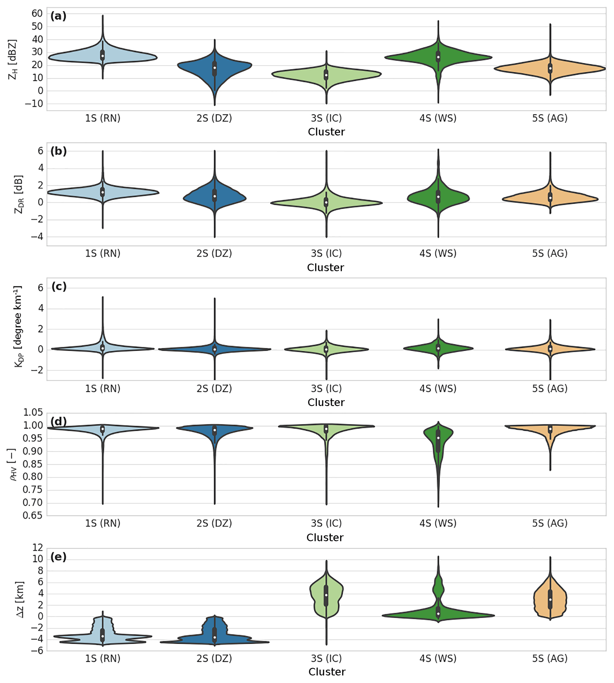
Figure 10Same as Fig. 7, but for the stratiform regime of the dry season (DZ is drizzle, RN is rain, WS is wet snow, AG is aggregates, and IC is ice crystals).
Table 5Same as Table 3, but for the stratiform region of the dry season.
The violin plots in Fig. 10 and contingency Table 5 allow discrimination and labelling of these clusters. For DR09 classification, clusters 1S and 2S exhibit rainfall signatures. Cluster 2S is in agreement with the fuzzy-logic drizzle category (∼92 %), whereas cluster 1S is divided into the drizzle (∼76 %) and rain (∼22 %) microphysical species. Between these two clusters, one can observe that cluster 1S contains the highest ZH, ZDR and KDP values, and one can consequently label it as a rainfall type. Cluster 2S is, however, associated with the drizzle/light-rain category according to the polarimetric radar signatures (GR15).
The liquid–solid delineation is represented here by cluster 4S. It presents a low ρHV (∼0.93) and a large ZH distribution around ∼30 dBZ and is almost only defined for altitudes close to the 0 ∘C isotherm. In addition, contingency Table 5 matches well with this hydrometeor association.
For the negative temperatures, the clustering outputs exhibit two clusters, 3S–5S. The first is located within the edge region of the cloud, whereas cluster 5S is distributed at lower altitudes and is closer to particles of greater densities (Fig. 10). Cluster 5S is in ∼70 % agreement with the aggregate fuzzy-logic outputs (Table 5), and its polarimetric signatures are close to those of GR15 and T-matrix simulations from DR09. One can then define cluster 5S as the aggregate microphysical species. Finally, ice crystals and small aggregates are represented through cluster 3S, which is defined by low ZH, ZDR, and KDP values and a high ρHV.
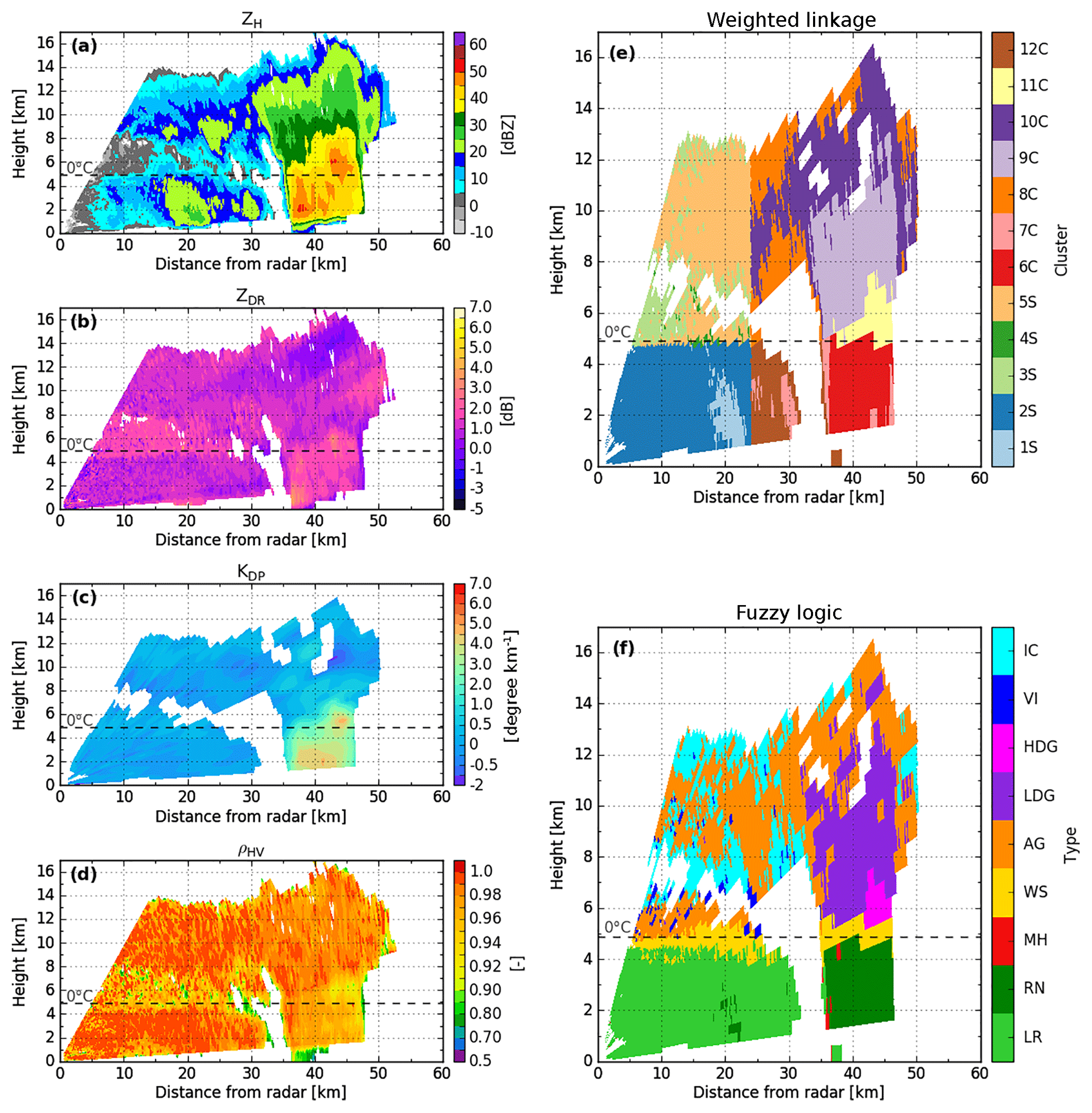
Figure 11Same as Fig. 9, but for an RHI at 18:16 UTC on 6 October 2014, along the azimuth 200∘.
5.2.2 Convective region
Figure 11 shows an RHI of a convective system that occurred in the late afternoon on 6 October 2014 in the region of Manaus. Overall, this RHI shows a convective cell (at 24–50 km from the radar) together with its relative stratiform region (0–23 km). Note that the abrupt transition from the convective and stratiform classification areas (Figs. 5, 6, 11) is inherent to the Steiner et al. (1995) algorithm. In terms of microphysical distribution, there should be some consistency between the two cloud types. The implementation of continuity analysis may prevent the latter artefacts. The convective cell is characterized by ZH values up to 25 dBZ at 14 km, and the cloud top exceeds 16 km. According to the fuzzy-logic outputs (Fig. 11f), the cell mostly exhibits rainfall precipitation for positive temperatures. The corresponding cluster outputs retrieve the same signatures, dividing the rain pattern into three different clusters: 6C, 7C, and 12C. Once again, the fuzzy logic collocates a bright band around the isotherm at 0 ∘C, whereas neither polarimetric signatures nor clustering outputs exhibit a bright band. For negative temperatures, the AHC method retrieves four clusters (8C, 9C, 10C, and 11C), the same as the fuzzy-logic outputs.
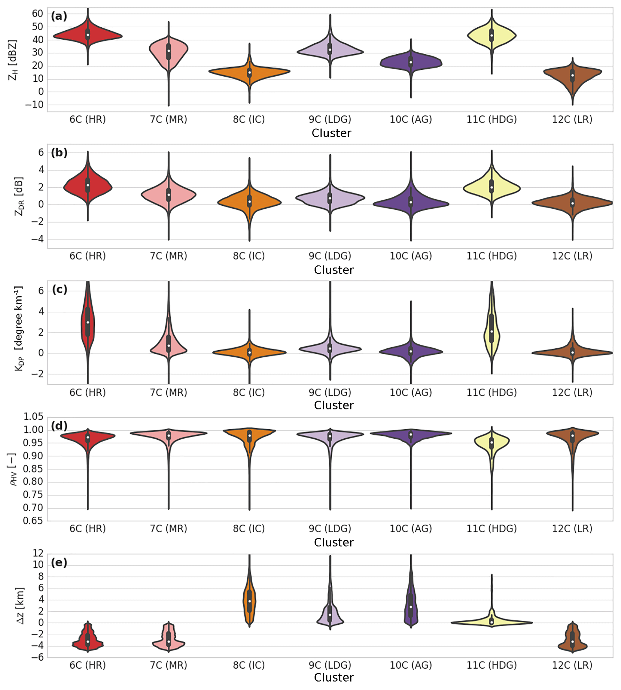
Figure 12Same as Fig. 7, but for the convective regime of the dry season (LR is light rain, MR is moderate rain, HR is heavy rain, LDG is low-density graupel, HDG is high-density graupel, AG is aggregates, and IC is ice crystals).
Table 6Same as Table 3, but for the stratiform region of the dry season.
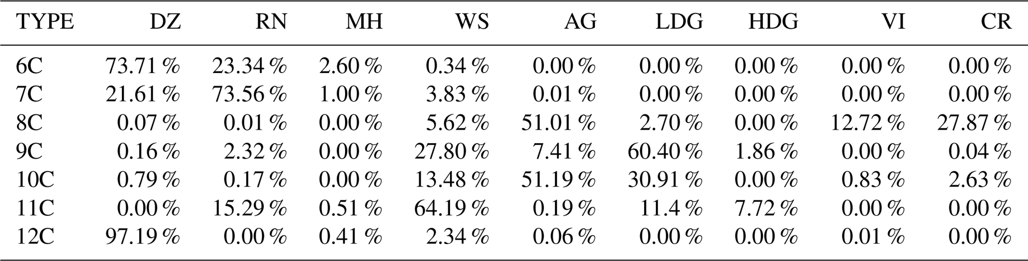
The violin plots in Fig. 12 and contingency Table 6 allow discrimination and labelling of these clusters. For the convective regions observed during the wet season, hail precipitation is rare in the Amazonas. Contingency Table 6 is also in agreement with this description, since none of the clustering outputs exceed 3 %. Therefore, one can attribute clusters 6C, 7C, and 12C to three different rainfall precipitation regimes, ranking the cluster positions as follows: 12C presents weaker ZH, ZDR, and KDP values than cluster 7C, which presents lower values than cluster 6C (Fig. 12). In addition, one can see from contingency Table 6 that all three are in very high agreement with the drizzle and rain microphysical species. Based on the aforementioned description together with the Fig. 11 analysis, one can attribute cluster 12C to light rainfall, cluster 7C to moderate rainfall and, finally, cluster 6C to the heavy-rainfall type.
Concerning all clusters spreading at negative temperatures, cluster 11C matches well with the high-density graupel category defined by DR09 such as “graupel growing in regions of large supercooled water contents, melting graupel, and freezing of supercooled rain”. Based on contingency Table 6, this cluster is mainly associated with wet snow and slightly with the low-density graupel microphysical specie. Nevertheless, one can see that the ρHV distribution is pretty low (∼0.94) and could also be the signature of wet graupel (due to melting or wet growth) or a mixture of graupel and hail, as suggested by Straka et al. (2000) and Kumjian and Ryzhkov (2008). This cloud region is surrounded by low-density graupel, characterized by cluster 9C (Figs. 11–12). This hydrometeor type shows 60 % agreement with this microphysical type within contingency Table 6 and is close to the DR09 T-matrix outputs. Cluster 10C shares more than 50 % with the aggregate type and 30 % with the low-density graupel type, whereas cluster 8C is associated in general with ice crystals and aggregate types (Table 6). With Figs. 11–12 and the aforementioned description, one can analyse cluster 9C as low-density graupel, cluster 10C as aggregates, and, finally, cluster 8C as ice crystals.
6.1 Impact of the clustering method and location
The present results allow us to make a brief comparison of the classical supervised fuzzy-logic technique commonly used in the literature and the unsupervised AHC method. In opposition to the rigid structure of a fuzzy-logic algorithm, the flexibility of the clustering approach allows better identification of the bright-band region. Indeed, the liquid–solid delineation around the 0 ∘C isotherm is better captured and distinguished by the AHC method, which preferentially follows the polarimetric signatures instead of the stratified temperature region. Additionally, one can see the ability of the AHC method to fully exploit the high sensitivity of the X-band radar frequency to distinguish between three different (light, moderate, and heavy) rainfall regimes such as in GR15. This enhancement allows, for instance, for more emphasis on severe convective precipitation cells and may open new perspectives for nowcasting issues.
Note that the present clustering method has been distinctly subdivided into stratiform and convective regions. Although they are characterized by different thermodynamic structures (Houze, 1997), the stratiform and convective regions may be related in terms of microphysical distributions, such as ice particles which might be ejected from the top of an active convective cell into the upper part of the stratiform region. This microphysical continuity could be further considered either by merging stratiform and convective hydrometeor types that present close DPOL characteristics (Figs. 7, 8, 10, and 12) or by implementing an a posteriori continuity analysis.
The location of the present study also offers the possibility of discussing midlatitude and tropical microphysical differences. As described in Sect. 5, the dominant tropical hydrometeor classification overlaps with some midlatitude microphysical species definitions. For instance, one can see that both the aggregate and ice crystal microphysical species are skewed to higher horizontal (differential) reflectivity, regardless of the season and region (stratiform/convective) considered. These discrepancies might be attributed either to an inaccurate attenuation correction or inherent tropical characteristics involved within microphysical ice growth. Although we considered a limited radar coverage, regions with high SNR values, as well as precipitation-only events having a dry radome, the ZPHI method may still lead to overcorrection, especially on ZDR in strong convective cases when the Mie scattering may dominate the precipitation regions. Another explanation of these discrepancies may rely on tropical atmospheric characteristics that present higher tropospheric humidity profiles together with higher incident solar radiation, playing an important role in comparison to midlatitudes.
6.2 Wet–dry season differences
The investigation of some Amazonian wet–dry season differences has already been explored by a few studies. For instance, Machado et al. (2018) noted that, during both the GoAmazon2014/5 and ACRIDICON-CHUVA field campaigns, the wet-season overall mean cumulative rain was 4 times as much as that during the dry season. However, though characterized by a low amount of total rainfall, the dry season presents the higher rainfall rate (Dolan et al., 2013; Machado et al., 2018). According to Machado et al. (2018), these discrepancies can partly be explained by the fact that the dry season presents higher convective available potential energy (CAPE) and lower cloud cover than the wet season. Another study conducted by Giangrande et al. (2017) also examined the wet–dry season differences through convective clouds. The authors showed that warm clouds exhibit larger cloud droplets and that the stratiform region during the wet season is much more developed than during the dry season (due to surrounding monsoon ambient characteristics).
All these differences are expected to contribute to the wet–dry season differences. Here, one can address for the first time these discrepancies through the dominant microphysical patterns in terms of stratiform and convection precipitation regimes associated with the Central Amazonas (Manaus region). Based on this new hydrometeor classification adapted to the tropical region, this section explores the differences among the clouds related to these two seasons.
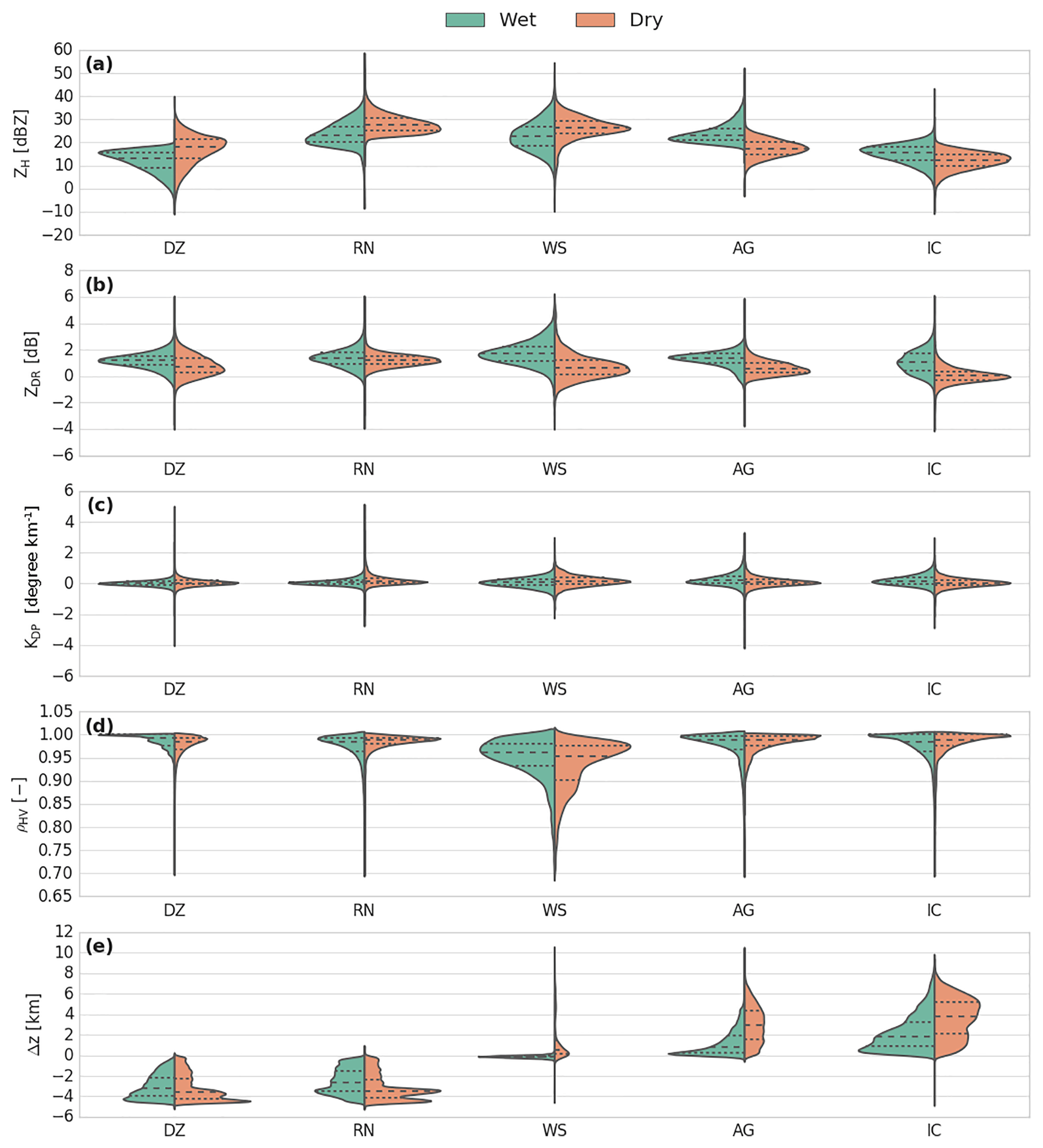
Figure 13Violin plot comparison of pairs of stratiform hydrometeor types between the wet and dry seasons (DZ is drizzle, RN is rain, WS is wet snow, AG is aggregates, and IC is ice crystals).
6.2.1 Stratiform region
Figure 13 presents a comparison of pairs of stratiform hydrometeor types between the wet and dry seasons. For positive temperatures, both the drizzle and rain microphysical species present higher ZH and lower ZDR values during the dry season than during the wet season. These polarimetric signatures might be attributed to the evaporation and collisional processes that tend to reduce the particle diameters (Kumjian and Ryzhkov, 2010; Penide et al., 2013). The separation between the drizzle/light rain and the rain microphysical species is defined for a rainfall rate of approximately 2.5 mm h−1 (American Meteorological Society, 2018). The classical Marshall–Palmer Z–R relationship allows an estimation of the rainfall rate for stratiform precipitation. In this regard, the wet-rain microphysical species is characterized, on average, by a rainfall rate of 1.84 mm h−1, whereas the rate is up to 3 mm h−1 during the dry season. The general wet-rain microphysical species distribution thus still contains drizzle/light-rain observations, which might be due to the different cloud cover patterns associated with stratiform echoes during the two seasons. As noted by Machado et al. (2018), stratiform cloud cover related to the rainy season is more associated with a monsoon cloud regime than during the remaining season. While the dry season stratiform regime is directly the result of the rain convective cells, the wet stratiform cover may also refer to large ambient unrelated residual precipitation far outside the original convective cloud.
Overall, the melting layer, which is represented here through the wet-snow microphysical species, is consistent with the results of previous studies (Durden et al., 1997; Giangrande et al., 2008; Heymsfield et al., 2015; Wolfensberger et al., 2016; Wang et al., 2018). The vertically restricted layer of wet snow presents the most widespread distribution of ZH, ZDR, KDP and ρHV of all the retrieved microphysical species and for both seasons. One can see that the wet-season distribution differs from the dry season, as its distribution is more associated with lower (higher) ZH (ZDR) values. The main discrepancy here is related to the ZDR distribution, which has stronger values during the wet season by approximately 1 dB. According to the study of Wang et al. (2018), which put emphasis onto mature mesoscale convective system events during the GoAmazon2014/5 experiment, the wet season always presents stronger bright-band signatures that might be attributed to more prominent aggregation processes. Indeed, the moist conditions at midlevels could promote more ice growth in the stratiform regions (as compared to the dry season) and could lead to stronger bright-band signatures when those aggregates melt.
One of the main differences in the cloud structure between the wet and dry season relies on the cloud-top altitudes. Indeed, during the dry season, clouds can easily reach 16–17 km in the tropics compared to only 13–14 km during the wet season. Therefore, the microphysical processes for negative temperatures are distributed over two different thickness layers and moisture profiles. In this cloud region, ice crystals grow by vapour diffusion until they have sufficient weight to start falling and forming aggregates (Houze, 1997). Although they present quite similar distributions, they both spread with about a 1.5 km interval difference in altitude. Additionally, the ZDR values associated with aggregates and ice crystals are generally slightly higher than those retrieved in DR09 or GR15. However, this result is consistent with the study of Wendisch et al. (2016), which identified shaped plates of aggregates and crystals in the anvil outflow with in situ airplane observations.
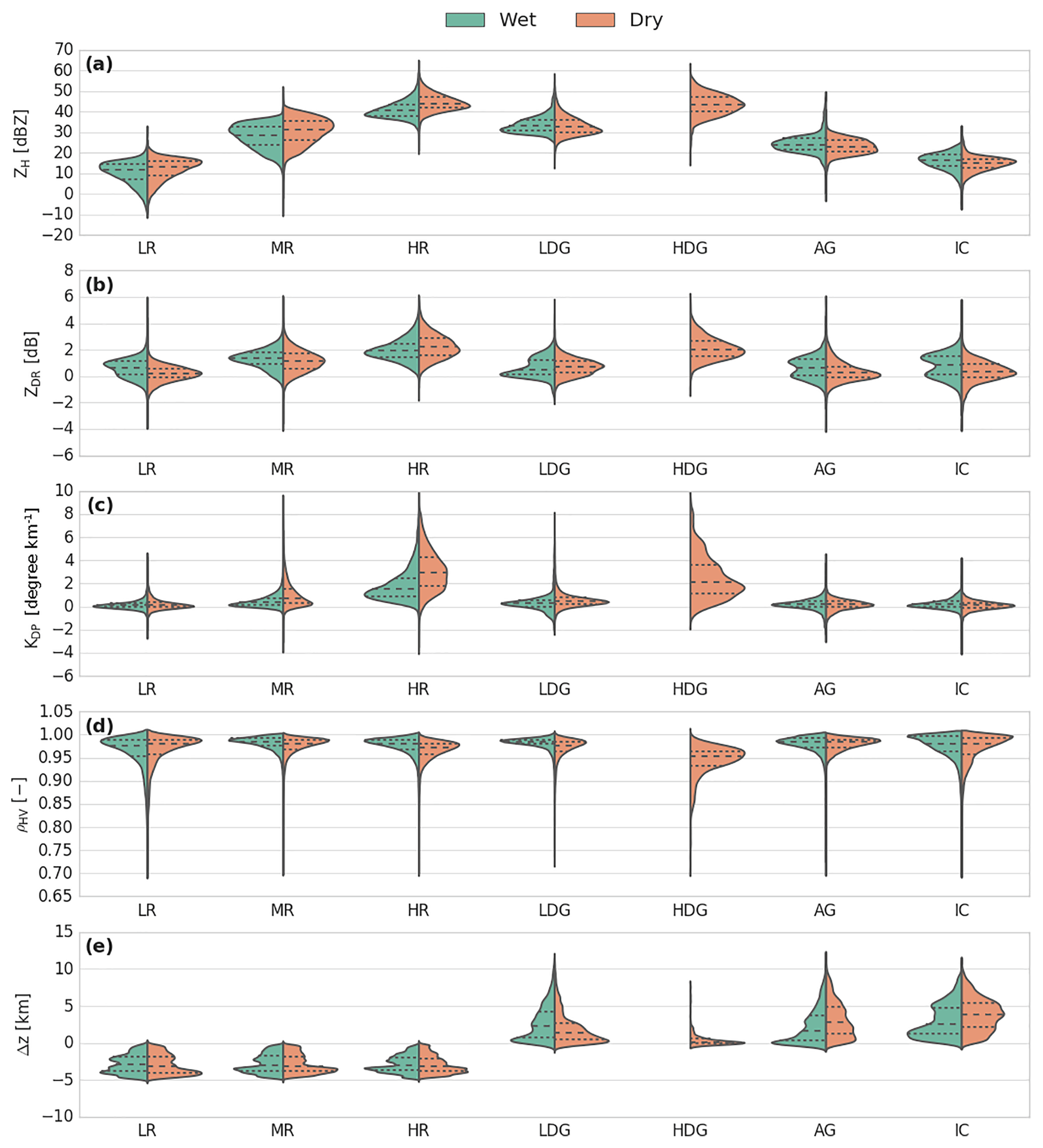
Figure 14Same as Fig. 13, but for the convective precipitation regime (LR is light rain, MR is moderate rain, HR is heavy rain, LDG is low-density graupel, HDG is high-density graupel, AG is aggregates, and IC is ice crystals).
6.2.2 Convective region
Figure 14 presents a comparison of pairs of convective microphysical species between the wet and dry seasons. As aforementioned in Sect. 5, the dry season is composed of seven hydrometeor types compared to six for the wet season. While the rainy season only has a graupel microphysical species, the dry season allows a distinction between low- and high-density graupel. Therefore, the graupel microphysical species defined during the wet season has been associated with the low-density graupel of the dry season to make this comparison possible.
Convective regions are characterized by three different rainfall regimes: light, moderate, and heavy rain. Overall, the ZH, ZDR, and KDP distributions associated with the dry season are generally shifted towards higher values. The dry season is known to exhibit the most intense convective cells (Machado et al., 2018). Their corresponding precipitation formation mechanism is generally dominated by ice microphysical processes, wherein the melting of graupel particles leads to large raindrops (Rosenfeld and Ulbrich, 2003; Dolan et al., 2013). One can see here that, although growth by coalescence could be very efficient during the wet season, the production of larger raindrops results mostly from ice microphysical processes.
Overall, the combination of the wet-season graupel microphysical species with the dry season low-density graupel makes sense in Fig. 14. Indeed, they have almost the same polarimetric range distributions and are in agreement with each other. By contrast, the high-density graupel signatures are correlated with high ZH, ZDR, and KDP values and low ρHV values. As mentioned in Sect. 5.2.2, high-density graupel would have been associated with a mixture of wet graupel and small hail. Nevertheless, these three related graupel categories are even consistent with the DR09 T-matrix definitions.
The main discrepancy between the aggregate and ice crystal microphysical species concerns their altitude definitions, wherein the dry season allows these hydrometeor types to be generated at higher altitudes. Systematically, the aggregate and ice crystal ZH and ZDR distributions are shifted to higher values during the wet season. These shifts may be due to an unreliable estimation of the attenuation correction or explained by the results of Rosenfeld and Lensky (1998) and Giangrande et al. (2017). Both of these studies showed that, during the dry season, updraughts are more intense and, therefore, do not allow enough time for small ice crystals to properly develop. In terms of aerosol concentrations, the wet Amazonian season is known to be much cleaner than the dry season (Artaxo et al., 2002). With this regard, Williams et al. (2002), Cecchini et al. (2017), or even Braga et al. (2017) highlighted its impact on the microphysical development of tropical cloud particles, showing that high aerosol concentrations may lead to smaller liquid particles within strong updraught regions. Small drops are known to freeze at colder temperatures by inhibiting the ice multiplication processes (Hallet and Mossop, 1974), and may account for the wet–dry season differences observed.
Based on an innovative clustering approach, the first hydrometeor classification for Amazon tropical-equatorial precipitation systems has been realized by using research X-band DPOL radar deployed during both the GoAmazon2014/5 and ACRIDICON-CHUVA field experiments. The AHC method was broadly equivalent to GR15 and built using ZH, ZDR, KDP and pHV polarimetric radar variables together with temperature information extracted from sounding balloons. The clustering approach allowed of polarimetric radar observations to be gathered that exhibit similarities within both wet and dry seasons and both stratiform and convective regions. Sensitivity analysis during the wet season was performed through different linkage rules and showed that both the weighted and Ward linkage rules were the most suitable for this hydrometeor classification task. In this regard, a novel approach was tested to improve the 0 ∘C hydrometeor layer representation within the convective region. While the 0 ∘C isotherm region is generally binarily represented, one can allow the liquid water content to overpass this region by setting simple rules. The final representation showed a realistic distribution and created new perspectives to respect polarimetric radar signatures as much as possible.
The AHC clustering outputs for both the wet and dry seasons and the stratiform and convective regions were investigated over the Manaus region with the complete datasets collected during 2014. Although previous studies were conducted for different latitudes and/or wavelengths, the retrieved hydrometeor types were found to be generally in agreement. Overall, typical cloud microphysical distributions within the stratiform precipitation regimes are characterized by five hydrometeors: drizzle/light rain, rain, wet snow, aggregates, and ice crystals. On the other hand, convective regions exhibit more diversified microphysical populations with six (seven) retrieved hydrometeor types for the wet (dry) season: light rain, moderate rain, heavy rain, low-density graupel, (high-density graupel), aggregates, and ice crystals.
The present study also highlighted the potential of the clustering approach in comparison to a more “classical” supervised fuzzy-logic algorithm. For instance, the clustering results showed a better ability to delimit and distinguish the bright-band region. The AHC method also allowed the higher sensitivity of the X-band radar to be exploited and permitted the retrieval of three different rainfall regimes by exhibiting light, moderate, and heavy intensities.
The retrieved labelled clusters allowed comparisons of the dominant microphysical species involved during both the wet and dry seasons of Brazilian tropical precipitation systems. Thus, the main discrepancy relies on the presence of one more microphysical species within the convective region of the dry season, defined as high-density graupel. This microphysical species is probably the result of a deeper convection associated with precipitation systems that occur during this period of the year.
Overall, the dry season ZH, ZDR, and KDP distribution shapes were quite similar to those of the rainy period; however, the distributions were shifted towards higher (lower) values for positive (negative) temperatures. The different rainfall intensities associated with the dry season generally exhibited higher ZH, ZDR, and KDP values than those during the wet season, leading us to believe that ice microphysical processes outweigh warm-rain microphysical mechanisms. Finally, the retrieved tropical microphysical species distribution showed that both aggregates and ice crystals were shifted towards higher radar observable values in comparison to the midlatitude X-band definition. These signatures might be due to the presence of a higher humidity amount within tropical regions, which may allow more dendritic-plate growth of aggregate and ice crystal microphysical species.
Although the year 2014 was representative and complied with typical tropical precipitation events, the present study could be strengthened by an extended dataset as well as the use of (i) in situ observations for validation tasks and (ii) aerosol information to investigate microphysical differences between the wet and dry season. Nevertheless, this first detailed analysis of dominant hydrometeor distributions within tropical precipitation systems is promising and could also be extended to other radar frequencies and operational DPOL radars. Such improvements could be useful for identifying key microphysical parameters for nowcasting issues, which are expected to be investigated in the near future through both the SOS-CHUVA (Brazil) and RELAMPAGO (Argentina) research projects. In this regard, the clustering methodology could be enhanced by taking into account the Doppler velocities to explore the microphysical processes involved within vigorous updraught and downdraught regions of the cloud. Finally, these results could also be helpful in evaluating the microphysical parameterization schemes used within high-resolution numerical weather prediction models.
The data set used in this study was collected during the GoAmazon2014/5 field experiment, which is part of the CHUVA project. Data can be accessed through the CHUVA portal (http://chuvaproject.cptec.inpe.br/, last access: 1 February 2019) or through the ARM Research Facility and the dedicated GoAmazon2014/5 field experiment archive (https://iop.archive.arm.gov/arm-iop/2014/mao/goamazon/T3/biscaro-xband_radar/, last access: 1 February 2019).
JFR and LATM developed the concept of the paper. JFR designed the radar methodology, performed the analyses, and interpreted the results. LATM contributed to the design and discussion of the work. TB contributed to the radar data processing part. JFR, with contributions from all authors, prepared the manuscript.
The authors declare that they have no conflict of interest.
This article is part of the special issue “Observations and Modeling of the Green Ocean Amazon (GoAmazon2014/5) (ACP/AMT/GI/GMD inter-journal SI)”. It is not associated with a conference.
The authors would like to especially thank Jacopo Grazioli for fruitful
discussions about the clustering method that helped refine the ideas
developed in this study. The contribution of the first author was supported
by the São Paulo Research Foundation (FAPESP) under grants 2016/16932-8
and 2015/14497-0 for the SOS-CHUVA project. Also, the ACRIDICON-CHUVA
campaign was partly funded by the German Research Foundation (Deutsche
Forschungsgemeinschaft, DFG Priority Program SPP 1294).
Edited by: Laura Bianco
Reviewed by: two anonymous referees
Al-Sakka, H., Boumahmoud, A. A., Fradon, B., Frasier, S. J., and Tabary, P.: A New Fuzzy Logic Hydrometeor Classification Scheme Applied to the French X-, C-, and S-Band Polarimetric Radars, J. Appl. Meteor. Climatol., 52, 2328–2344, 2013.
American Meteorological Society: Rain. Glossary of Meteorology, available at: http://glossary.ametsoc.org/wiki/rain, last access: 2018.
Artaxo, P., Martins, J. V., Yamasoe, M. A., Procópio, A. S., Pauliquevis, T. M., Andreae, M. O., Guyon, P., Gatti, L. V., and Leal, A. M.: Physical and chemical properties of aerosols in the wet and dry seasons in Rondônia, Amazonia, J. Geophys. Res.-Atmos., 107, 8081, https://doi.org/10.1029/2001JD000666, 2002.
Augros, C., Caumont, O., Ducrocq, V., Gaussiat, N., and Tabary, P.: Comparisons between S-, C-and X-band polarimetric radar observations and convective-scale simulations of the HyMeX first special observing period, Q. J. Roy. Meteor. Soc., 142, 347–362, 2016.
Aydin, K., Seliga, T. A., and Balaji, V.: Remote sensing of hail with a dual linear polarization radar, J. Clim. Appl. Meteorol., 25, 1475–1484, 1986.
Bechini, R. and Chandrasekar V.: A Semisupervised Robust Hydrometeor Classification Method for Dual-Polarization Radar Applications, J. Atmos. Ocean. Tech., 32, 22–47, https//doi.org/10.1175/JTECH-D-14-00097.1, 2015.
Bechini, R., Chandrasekar, V., Cremonini, R., and Lim, S.: Radome attenuation at X-band radar operations, Proc. Sixth European Conf. on Radar in Meteorology and Hydrology, Sibiu, Romania, ERAD, p. 15.1, available at: http://www.erad2010.org/pdf/POSTER/Thursday/02_Xband/01_ERAD2010_0346_extended.pdf (last access: November 2016), 2010.
Besic, N., Figueras i Ventura, J., Grazioli, J., Gabella, M., Germann, U., and Berne, A.: Hydrometeor classification through statistical clustering of polarimetric radar measurements: a semi-supervised approach, Atmos. Meas. Tech., 9, 4425–4445, https://doi.org/10.5194/amt-9-4425-2016, 2016.
Braga, R. C., Rosenfeld, D., Weigel, R., Jurkat, T., Andreae, M. O., Wendisch, M., Pöschl, U., Voigt, C., Mahnke, C., Borrmann, S., Albrecht, R. I., Molleker, S., Vila, D. A., Machado, L. A. T., and Grulich, L.: Further evidence for CCN aerosol concentrations determining the height of warm rain and ice initiation in convective clouds over the Amazon basin, Atmos. Chem. Phys., 17, 14433–14456, https://doi.org/10.5194/acp-17-14433-2017, 2017.
Bringi, V. N. and Chandrasekar V.: Polarimetric Doppler weather radar: principles and applications, Cambridge University Press, Cambridge, UK, 2001.
Bringi, V. N., Rasmussen, R. M., and Vivekanandan, J.: Multiparameter radar measurements in Colorado convective storms. Part I: Graupel melting studies, J. Atmos. Sci., 43, 2545–2563, 1986.
Bringi, V. N., Thurai, R., and Hannesen, R.: Dual-Polarization Weather Radar Handbook, AMS-Gematronik GmbH, Germany, 2007.
Cazenave, F., Gosset, M., Kacou, M., Alcoba, M., Fontaine, E., Duroure, C., and Dolan, B.: Characterization of hydrometeors in Sahelian convective systems with an X-band radar and comparison with in situ measurements. Part I: Sensitivity of polarimetric radar particle identification retrieval and case study evaluation, J. Appl. Meteorol. Clim., 55, 231–249, 2016.
Cecchini, M. A., Machado, L. A. T., Wendisch, M., Costa, A., Krämer, M., Andreae, M. O., Afchine, A., Albrecht, R. I., Artaxo, P., Borrmann, S., Fütterer, D., Klimach, T., Mahnke, C., Martin, S. T., Minikin, A., Molleker, S., Pardo, L. H., Pöhlker, C., Pöhlker, M. L., Pöschl, U., Rosenfeld, D., and Weinzierl, B.: Illustration of microphysical processes in Amazonian deep convective clouds in the gamma phase space: introduction and potential applications, Atmos. Chem. Phys., 17, 14727–14746, https://doi.org/10.5194/acp-17-14727-2017, 2017.
Dolan, B. and Rutledge, S. A.: A Theory-Based Hydrometeor Identification Algorithm for X-Band Polarimetric Radars, J. Atmos. Ocean. Tech., 26, 2071–2088, 2009.
Dolan, B., Rutledge, S. A., Lim, S., Chandrasekar, V., and Thurai, M.: A robust C-Band hydrometeor identification algorithm and application to a long-term polarimetric radar dataset, J. Appl. Meteorol. Clim., 52, 2162–2186, 2013.
Durden, S. L., Kitlyakara, A., Im, E., Tanner, A. B., Haddad, Z. S., Li, F. K., and Wilson, W. J.: ARMAR observations of the melting layer during TOGA COARE, IEEE T. Geosci. Remote, 35, 1453–1456, 1997.
El-Magd, A., Chandrasekar, V., Bringi, V., and Strapp, W.: Multiparameter radar and in situ aircraft observation of graupel and hail, IEEE T. Geosci. Remote, 38, 570–578, 2000.
Giangrande, S. E., Krause, J. M., and Ryzhkov, A. V.: Automatic designation of the melting layer with a polarimetric prototype of the WSR-88D radar, J. Appl. Meteorol. Clim., 47, 1354–1364, 2008.
Giangrande, S. E., Toto, T., Jensen, M. P., Bartholomew, M. J., Feng, Z., Protat, A., Williams, C. R., Schumacher, C., and Machado, L.: Convective cloud vertical velocity and mass-flux characteristics from radar wind profiler observations during GoAmazon2014/5, J. Geophys. Res.-Atmos., 121, 12891–12913, https://doi.org/10.1002/2016JD025303, 2017.
Grazioli, J., Tuia, D., and Berne, A.: Hydrometeor classification from polarimetric radar measurements: a clustering approach, Atmos. Meas. Tech., 8, 149–170, https://doi.org/10.5194/amt-8-149-2015, 2015.
Grazioli, J., Genthon, C., Boudevillain, B., Duran-Alarcon, C., Del Guasta, M., Madeleine, J.-B., and Berne, A.: Measurements of precipitation in Dumont d'Urville, Adélie Land, East Antarctica, The Cryosphere, 11, 1797–1811, https://doi.org/10.5194/tc-11-1797-2017, 2017.
Hall, M. P. M., Goddard, J. W. F., and Cherry, S. M.: Identification of hydrometeors and other targets by dual-polarization radar, Radio Sci., 19, 132–140, 1984.
Hallett, J. and Mossop, S. C. C.: Production of secondary ice particles during the riming process, Nature, 249, 26–28, 1974.
Heymsfield, A. J., Bansemer, A., Poellot, M. R., and Wood, N.: Observations of Ice Microphysics through the Melting Layer, J. Atmos. Sci., 72, 2902–2928, https://doi.org/10.1175/JAS-D-14-0363.1, 2015.
Höller, H., Hagen, M., Meischner, P. F., Bringi, V. N., and Hubbert, J.: Life Cycle and Precipitation Formation in a Hybrid-Type Hailstorm Revealed by Polarimetric and Doppler Radar Measurements, J. Atmos. Sci., 51, 2500–2522, 1994.
Houze, R. A.: Stratiform Precipitation in Regions of Convection: A Meteorological Paradox?, B. Am. Meteorol. Soc., 78, 2179–2196, https://doi.org/10.1175/1520-0477(1997)078<2179:SPIROC>2.0.CO;2, 1997.
Hubbert, J. and Bringi, V. N.: An iterative filtering technique for the analysis of copolar differential phase and dual-frequency radar measurements, J. Atmos. Ocean. Tech., 12.3, 643–648, 1995.
Illingworth, A. J. and Blackman, T. M.: The need to represent raindrop size spectra as normalized gamma distributions for the interpretation of polarization radar observations, J. Appl. Meteorol., 41, 286–297, 2002.
Jain, A. K., Duin, R. P. W., and Mao, J. C.: Statistical pattern recognition: A review, IEEE T. Pattern Analysis Machine Intell., 22, 4–37, https://doi.org/10.1109/34.824819, 2000.
Jäkel, E., Wendisch, M., Krisna, T. C., Ewald, F., Kölling, T., Jurkat, T., Voigt, C., Cecchini, M. A., Machado, L. A. T., Afchine, A., Costa, A., Krämer, M., Andreae, M. O., Pöschl, U., Rosenfeld, D., and Yuan, T.: Vertical distribution of the particle phase in tropical deep convective clouds as derived from cloud-side reflected solar radiation measurements, Atmos. Chem. Phys., 17, 9049–9066, https://doi.org/10.5194/acp-17-9049-2017, 2017.
Kumjian, M. R. and Ryzhkov, A. V.: Polarimetric Signatures in Supercell Thunderstorms, J. Appl. Meteorol. Clim., 47, 1940–1961, https://doi.org/10.1175/2007JAMC1874.1, 2008.
Kumjian, M. R. and Ryzhkov, A. V.: The impact of evaporation on polarimetric characteristics of rain: Theoretical model and practical implications, J. Appl. Meteorol. Clim., 49, 1247–1267, 2010.
Leary, C. A. and Houze Jr., R. A.: Melting and evaporation of hydrometeors in precipitation from the anvil clouds of deep tropical convection, J. Atmos. Sci., 36, 669–679, 1979.
Liu, H. and Chandrasekar, V.: Classification of Hydrometeors Based on Polarimetric Radar Measurements: Development of Fuzzy Logic and Neuro-Fuzzy Systems, and In Situ Verification, J. Atmos. Ocean. Tech., 17, 140–164, 2000.
Machado, L. A. T., Calheiros, A. J. P., Biscaro, T., Giangrande, S., Silva Dias, M. A. F., Cecchini, M. A., Albrecht, R., Andreae, M. O., Araujo, W. F., Artaxo, P., Borrmann, S., Braga, R., Burleyson, C., Eichholz, C. W., Fan, J., Feng, Z., Fisch, G. F., Jensen, M. P., Martin, S. T., Pöschl, U., Pöhlker, C., Pöhlker, M. L., Ribaud, J.-F., Rosenfeld, D., Saraiva, J. M. B., Schumacher, C., Thalman, R., Walter, D., and Wendisch, M.: Overview: Precipitation characteristics and sensitivities to environmental conditions during GoAmazon2014/5 and ACRIDICON-CHUVA, Atmos. Chem. Phys., 18, 6461–6482, https://doi.org/10.5194/acp-18-6461-2018, 2018.
Martin, S. T., Artaxo, P., Machado, L. A. T., Manzi, A. O., Souza, R. A. F., Schumacher, C., Wang, J., Andreae, M. O., Barbosa, H. M. J., Fan, J., Fisch, G., Goldstein, A. H., Guenther, A., Jimenez, J. L., Pöschl, U., Silva Dias, M. A., Smith, J. N., and Wendisch, M.: Introduction: Observations and Modeling of the Green Ocean Amazon (GoAmazon2014/5), Atmos. Chem. Phys., 16, 4785–4797, https://doi.org/10.5194/acp-16-4785-2016, 2016.
Martin, S. T., Artaxo, P., Machado, L., Manzi, A. O., Souza, R. A., Schumacher, C., Wang, J., Biscaro, T., Brito, J., Calheiros, A., Jardine, K., Medeiros, A., Portela, B., de Sá, S. S., Adachi, K., Aiken, A. C., Albrecht, R., Alexander, L., Andreae, M. O., Barbosa, H. M., Buseck, P., Chand, D., Comstock, J. M., Day, D. A., Dubey, M., Fan, J., Fast, J., Fisch, G., Fortner, E., Giangrande, S., Gilles, M., Goldstein, A. H., Guenther, A., Hubbe, J., Jensen, M., Jimenez, J. L., Keutsch, F. N., Kim, S., Kuang, C., Laskin, A., McKinney, K., Mei, F., Miller, M., Nascimento, R., Pauliquevis, T., Pekour, M., Peres, J., Petäjä, T., Pöhlker, C., Pöschl, U., Rizzo, L., Schmid, B., Shilling, J. E., Dias, M. A., Smith, J. N., Tomlinson, J. M., Tóta, J., and Wendisch, M.: The Green Ocean Amazon Experiment (GoAmazon2014/5) Observes Pollution Affecting Gases, Aerosols, Clouds, and Rainfall over the Rain Forest, B. Am. Meteorol. Soc., 98, 981–997, 2017.
Marzano, F., Scaranari, D., Celano, M., Alberoni, P. P., Vulpiani, G., and Montopoli, M.: Hydrometeor classification from dual-polarized weather radar: extending fuzzy logic from S-band to C-band data, Adv. Geosci., 7, 109–114, 2006.
Marzano, F., Scaranari, D., Montopoli, M., and Vulpiani, G.: Supervised classification and estimation of hydrometeors from C-band dual-polarized radars: A Bayesian approach, IEEE T. Geosci. Remote, 46, 85–98, https://doi.org/10.1109/TGRS.2007.906476, 2008.
Marzano, F. S., Botta, G., and Montopoli, M.: Iterative Bayesian retrieval of hydrometeor content from X-band polarimetric weather radar, IEEE T. Geosci. Remote, 48, 3059–3074, 2010.
Matrosov, S. Y., Clark, K. A., and Kingsmill, D. E.: A polarimetric radar approach to identify rain, melting-layer, and snow regions for applying corrections to vertical profiles of reflectivity, J. Appl. Meteorol. Clim., 46, 154–166, 2007.
Mendel, J. M.: Fuzzy logic systems for engineering: A tutorial, Proc. IEEE, 83, 345–377, 1995.
Mishchenko, M. I. and Travis, L. D.: Capabilities and limitations of a current Fortran implementation of the T-Matrix method for randomly oriented, rotationally symmetric scatterers, J. Quant. Spectr. Ra., 60, 309–324, 1998.
Müllner, D.: Modern hierarchical, agglomerative clustering algorithms, arXiv preprint, arXiv:1109.2378, 2011.
Oliveira, R., Maggioni, V., Vila, D., and Morales, C.: Characteristics and diurnal cycle of GPM rainfall estimates over the central amazon region, Remote Sens., 8, 544, 2016.
Park, H. S., Ryzhkov, A. V., Zrnić, D., and Kim, K. E.: The Hydrometeor Classification Algorithm for the Polarimetric WSR-88D: Description and Application to an MCS, Weather Forecast., 24, 730–748, 2009.
Penide, G., Kumar, V. V., Protat, A., and May, P. T.: Statistics of drop size distribution parameters and rain rates for stratiform and convective precipitation during the north Australian wet season, Mon. Weather Rev., 141, 3222–3237, 2013.
Ribaud, J.-F., Bousquet, O., and Coquillat, S.: Relationships between total lightning activity, microphysics and kinematics during the 24 September 2012 HyMeX bow-echo system, Q. J. Roy. Meteor. Soc., 142, 298–309, 2016a.
Ribaud, J.-F., Bousquet, O., Coquillat, S., Al-Sakka, H., Lambert, D., Ducrocq, V., and Fontaine, E.: Evaluation and application of hydrometeor classification algorithm outputs inferred from multi-frequency dual-polarimetric radar observations collected during HyMeX, Q. J. Roy. Meteor. Soc., 142, 95–107, https://doi.org/10.1002/qj.2589, 2016b.
Rosenfeld, D. and Lensky, I. M.: Satellite-based insights into precipitation formation processes in continental and maritime convective clouds, B. Am. Meteorol. Soc., 79, 2457–2476, 1998.
Rosenfeld, D. and Ulbrich, C. W.: Cloud microphysical properties, processes, and rainfall estimation opportunities. Radar and Atmospheric Science: A Collection of Essays in Honor of David Atlas, Meteor. Monogr., 52, 237–258, 2003.
Ryzhkov, A. V., Schuur, T. J., Burgess, D. W., Heinselman, P. L., Giangrande, S. E., and Zrnic, D. S.: The joint polarization experiment, polarimetric rainfall measurements and hydrometeor classification, B. Am. Meteorol. Soc., 86, 809–824, https://doi.org/10.1175/BAMS-86-6-809, 2005.
Ryzhkov, A. V., Kumjian, M. R., Ganson, S. M., and Khain, A. P.: Polarimetric radar characteristics of melting hail. Part I: Theoretical simulations using spectral microphysical modeling, J. Appl. Meteorol. Clim., 52, 2849–2870, 2013.
Schneebeli, M., Sakuragi, J., Biscaro, T., Angelis, C. F., Carvalho da Costa, I., Morales, C., Baldini, L., and Machado, L. A. T.: Polarimetric X-band weather radar measurements in the tropics: radome and rain attenuation correction, Atmos. Meas. Tech., 5, 2183–2199, https://doi.org/10.5194/amt-5-2183-2012, 2012.
Segond, M.-L., Tabary, P., and Parent du Châtelet, J.: Quantitative precipitation estimations from operational polarimetric radars for hydrological applications, Preprints, 33rd Int. Conf. on Radar Meteorology, AMS, Cairns, Australia, August 2007.
Seliga, T. A. and Bringi, V. N.: Potential use of radar differential reflectivity measurements at orthogonal polarizations for measuring precipitation, J. Appl. Meteorol., 15, 69–76, https://doi.org/10.1175/1520-0450(1976)015%3C0069:PUORDR%3E2.0.CO;2, 1976.
Smyth, T. J. and Illingworth, A. J.: Radar estimates of rainfall rates at the ground in bright band and non-bright band events, Q. J. Roy. Meteor. Soc., 124, 2417–2434, 1998.
Steiner, M., Houze Jr., R. A., and Yuter, S. E.: Climatological characterization of three-dimensional storm structure from operational radar and rain gauge data, J. Appl. Meteorol., 34, 1978–2007, 1995.
Straka, J. M.: Hydrometeor fields in a supercell storm as deduced from dual polarization radar. Preprints, 18th Conf. on Severe Local Storms, San Francisco, CA, Amer. Meteor. Soc., 551–554, 1996.
Straka, J. and Zrnić, D. S.: An algorithm to deduce hydrometeor types and contents from multiparameter radar data, Preprints, 26th Conf. on Radar Meteorology, Norman, OK, Amer. Meteor. Soc., 513–515, 1993.
Straka, J. M., Zrnić, D. S., and Ryzhkov, A. V.: Bulk hydrometeor classification and quantification using polarimetric radar data: Synthesis of relations, J. Appl. Meteorol., 39.8, 1341–1372, 2000.
Testud, J., Le Bouar, E., Obligis, E., and Ali-Meheni, M.: The rain profiling algorithm applied to polarimetric weather radar, J. Atmos. Ocean. Tech., 17, 332–356, 2000.
Thompson, E. J., Rutledge, S. A., Dolan, B., Chandrasekar, V., and Cheong, B. L.: A dual-polarization radar hydrometeor classification algorithm for winter precipitation, J. Atmos. Ocean. Tech., 31, 1457–1481, https://doi.org/10.1175/JTECH-D-13-00119.1, 2014.
Vivekanandan, J., Ellis, S. M., Oye, R., Zrnić, D. S., Ryzhkov, A. V., and Straka, J.: Cloud Microphysics Retrieval Using S-band Dual-Polarization Radar Measurements, B. Am. Meteorol. Soc., 80, 381–388, 1999.
Wang, D., Giangrande, S. E., Bartholomew, M. J., Hardin, J., Feng, Z., Thalman, R., and Machado, L. A. T.: The Green Ocean: precipitation insights from the GoAmazon2014/5 experiment, Atmos. Chem. Phys., 18, 9121–9145, https://doi.org/10.5194/acp-18-9121-2018, 2018.
Ward, J.: Hierarchical grouping to optimize an objective function, J. Am. Stat. Assoc., 58, 236–244, 1963.
Wen, G., Protat, A., May, P. T., Wang, X., and Moran, W.: A cluster-based method for hydrometeor classification using polarimetric variables. Part I: Interpretation and analysis, J. Atmos. Ocean. Tech., 32, 1320–1340, 2015.
Wen, G., Protat, A., May, P. T., Moran, W., and Dixon, M.: A cluster-based method for hydrometeor classification using polarimetric variables. Part II: Classification, J. Atmos. Ocean. Tech., 33, 45–60, 2016.
Wendisch, M., Pöschl, U., Andreae, M. O., Machado, L. A. T., Albrecht, R., Schlager, H., Rosenfeld, D., Martin, S. T., Abdelmonem, A., Afchine, A., Araújo, A., Artaxo, P., Aufmhoff, H., Barbosa, H. M. J., Borrmann, S., Braga, R., Buchholz, B., Cecchini, M. A., Costa, A., Curtius, J., Dollner, M., Dorf, M., Dreiling, V., Ebert, V., Ehrlich, A., Ewald, F., Fisch, G., Fix, A., Frank, F., Fütterer, D., Heckl, C., Heidelberg, F., Hüneke, T., Jäkel, E., Járvinen, E., Jurkat, T., Kanter, S., Kästner, U., Kenntner, M., Kesselmeier, J., Klimach, T., Knecht, M., Kohl, R., Kölling, T., Krämer, M., Krüger, M., Krisna, T. C., Lavric, J. V., Longo, K., Mahnke, C., Manzi, A. O., Mayer, B., Mertes, S., Minikin, A., Molleker, S., Münch, S., Nillius, B., Pfeilsticker, K., Pöhlker, C., Roiger, A., Rose, D., Rosenow, D., Sauer, D., Schnaiter, M., Schneider, J., Schulz, C., de Souza, R. A. F., Spanu, A., Stock, P., Vila, D., Voigt, C., Walser, A., Walter, D., Weigel, R., Weinzierl, B., Werner, F., Yamasoe, M. A., Ziereis, H., Zinner, T., and Zöger, M.: The ACRIDICON-CHUVA campaign: Studying tropical deep convective clouds and precipitation over Amazonia using the new German research aircraft HALO, B. Am. Meteorol. Soc., 97, 1885–1908, https://doi.org/10.1175/BAMS-D-14-00255.1, 2016.
Williams, E., Rosenfeld, D., Madden, N., Gerlach, J., Gears, N., Atkinson, L., Dunnemann, N., Frostrom, G., Antonio, M., Biazon, B., and Camargo, R.: Contrasting convective regimes over the Amazon: Implications for cloud electrification, J. Geophys. Res.-Atmos., 27, 107, LBA-50, 2002.
Wolfensberger, D. and Berne, A.: From model to radar variables: a new forward polarimetric radar operator for COSMO, Atmos. Meas. Tech., 11, 3883–3916, https://doi.org/10.5194/amt-11-3883-2018, 2018.
Wolfensberger, D., Scipion, D., and Berne, A.: Detection and characterization of the melting layer based on polarimetric radar scans, Q. J. Roy. Meteor. Soc., 142, 108–124, 2016.
Zrnić, D. S., Ryzhkov, A., Straka, J., Liu, Y., and Vivekanandan, J.: Testing a procedure for automatic classification of hydrometeor types, J. Atmos. Ocean. Tech., 18, 892–913, https://doi.org/10.1175/1520-0426(2001)018%3C0892:TAPFAC%3E2.0.CO;2, 2001.
- Abstract
- Introduction
- Datasets and processing
- Unsupervised agglomerative hierarchical clustering
- Methodology discussions
- Wet- and dry-season-dominant hydrometeor classifications
- Discussion
- Conclusions
- Data availability
- Appendix A: Wet- and dry-season cluster centroids
- Author contributions
- Competing interests
- Special issue statement
- Acknowledgements
- References