the Creative Commons Attribution 4.0 License.
the Creative Commons Attribution 4.0 License.
 | 12 Feb 2019
Enhancing the spatiotemporal features of polar mesosphere summer echoes using coherent MIMO and radar imaging at MAARSY
Juan Miguel Urco
Jorge Luis Chau
Tobias Weber
Ralph Latteck
Polar mesospheric summer echoes (PMSEs) are very strong radar echoes caused by the presence of ice particles, turbulence, and free electrons in the mesosphere over polar regions. For more than three decades, PMSEs have been used as natural tracers of the complicated atmospheric dynamics of this region. Neutral winds and turbulence parameters have been obtained assuming PMSE horizontal homogeneity on scales of tens of kilometers. Recent radar imaging studies have shown that PMSEs are not homogeneous on these scales and instead they are composed of kilometer-scale structures. In this paper, we present a technique that allows PMSE observations with unprecedented angular resolution (∼0.6∘). The technique combines the concept of coherent MIMO (Multiple Input Multiple Output) and two high-resolution imaging techniques, i.e., Capon and maximum entropy (MaxEnt). The resulting resolution is evaluated by imaging specular meteor echoes. The gain in angular resolution compared to previous approaches using SIMO (Single Input Multiple Output) and Capon is at least a factor of 2; i.e., at 85 km, we obtain a horizontal resolution of ∼900 m. The advantage of the new technique is evaluated with two events of 3-D PMSE structures showing: (1) horizontal wavelengths of 8–10 km and periods of 4–7 min, drifting with the background wind, and (2) horizontal wavelengths of 12–16 km and periods of 15–20 min, not drifting with the background wind. Besides the advantages of the implemented technique, we discuss its current challenges, like the use of reduced power aperture and processing time, as well as the future opportunities for improving the understanding of the complex small-scale atmospheric dynamics behind PMSEs.
- Article
(8703 KB) -
Supplement
(28485 KB) - BibTeX
- EndNote


The so-called MIMO (Multiple Input Multiple Output) technique is being widely used in the fields of telecommunications and radar remote sensing (e.g Telatar, 1999; Huang et al., 2011; Foschini and Gans, 1998). Recently Urco et al. (2018) have shown that the use of multiple transmitters and multiple receivers can significantly improve the angular resolution of coherent atmospheric and ionospheric radars. In that work, MIMO was used to observe equatorial electrojet (EEJ) field-aligned irregularities at Jicamarca in combination with the well-established radar imaging technique Capon (e.g., Palmer et al., 1998). The multiple transmitter part was implemented with three different diversity schemes, i.e., temporal, code, and polarization. The resulting angular resolution was superior, by at least a factor of 4, to previous efforts using a single transmitter and the same receiving configuration, i.e., SIMO (Single Input Multiple Output). Given that the EEJ irregularities are field-aligned with the Earth's magnetic field, angular imaging was performed only in the magnetic east–west direction.
Based on this successful implementation, we decided to implement coherent MIMO to improve the angular resolution of the Middle Atmosphere ALOMAR Radar System (MAARSY) (16.04∘ E, 69.30∘ N) and to study polar mesospheric summer echoes (PMSEs). PMSEs present strong radar cross sections (RCSs) that allow them to be observed with less transmitting power, which is the case when using MIMO. Previous efforts to study their spatial structure have been limited to a few kilometers' spatial resolution and a few minutes' temporal resolution (e.g., Yu et al., 2001; Latteck et al., 2012a; Stober et al., 2013; Sommer and Chau, 2016). Recently, Stober et al. (2018) have presented many examples of monochromatic gravity waves (GWs) and Kelvin–Helmholtz instabilities (KHIs) using 9 days of multibeam PMSE observations with MAARSY.
PMSEs are strong echoes, more than 50 dB stronger than expected echoes from free electrons in the D region, and there is a consensus that they are generated by atmospheric turbulence and require the presence of free electrons and charged ice particles (e.g., Rapp et al., 2002; Varney et al., 2011, and references therein). Although PMSEs have been studied since the late 1970s (e.g., Ecklund and Balsley, 1981; Hoppe et al., 1988; Kelley and Ulwick, 1988; Havnes et al., 1996; Rapp and Lübken, 2004), until recently they have been considered very aspect-sensitive and homogeneous on scales of a few tens of kilometers, at least when observed at very high frequencies (VHFs) (e.g., Czechowsky et al., 1988; Zecha et al., 2001; Yu et al., 2001).
Based on recent multibeam observations as well as radar imaging, Sommer and Chau (2016) have concluded that the PMSEs are not as aspect-sensitive as previously reported, and instead, most of the time they are organized in kilometer-scale spatial structures drifting across the observing beams. Such results have been independently verified with bistatic observations at VHFs, where PMSEs were observed with small systems at zenith angles close to 30∘ (e.g., Chau et al., 2018).
The results of Sommer and Chau (2016) were obtained with MAARSY using the whole antenna array for transmitting and an antenna compression approach, i.e., a wide beam by properly phasing the antennas (e.g., Woodman and Chau, 2001) and a multiple-receiver configuration. The spatial structures were obtained using the Capon technique due to its implementation simplicity and its relatively fast processing speed.
Given that PMSEs are highly associated with noctilucent clouds (NLCs) (e.g., Hoppe et al., 1990; Stebel et al., 2000; Kaifler et al., 2011), spatial structures ranging from a few hundreds of meters to a few tens of kilometers observed in NLCs (e.g., Baumgarten and Fritts, 2014) are expected to be observed also in PMSEs. Indeed this is the case, PMSE structures of a few kilometers have been already reported by Sommer and Chau (2016) and structures of a few tens of kilometers have been reported by Chau et al. (2018).
Although progress has been made in discriminating between spatial and temporal ambiguities in PMSE observations, the achieved angular resolution has been mainly limited by two factors: (1) the effective area in the visibility plane and (2) the number of independent spatial samples (e.g., Woodman, 1997). By implementing MIMO, we are able to improve both, i.e., a larger effective area and a higher number of independent visibility samples. In addition, by implementing maximum entropy (MaxEnt), which is more computationally demanding than Capon, we are able to further improve the angular resolution (e.g., Hysell and Chau, 2006).
In this work, we have implemented coherent MIMO at MAARSY using 3 spatially separated antenna sections on transmission and 15 on reception. Moreover, time diversity was employed in order to isolate radar echoes corresponding to each transmitting section; i.e., the transmitters were interleaved every 4 ms. The resulting effective number of virtual receivers by using MIMO was 45 and the angular resolution achieved was ∼0.6∘. It is equivalent to an antenna area of 450 m diameter, more than 5 times larger than the nominal diameter of the MAARSY antenna.
Our paper is organized as follows. We first present the experiment configuration with a specific emphasis on the MIMO implementation. Then we describe the radar imaging implementation for both Capon and MaxEnt techniques. The PMSE results are shown in Sect. 4 for SIMO and MIMO using both Capon and MaxEnt. Within this section, two events are studied in detail, one in which the observed waves drift with the background wind and a second one in which the waves do not propagate with the wind. Finally, the results of our MIMO implementation are discussed, followed by conclusions.
2.1 MAARSY
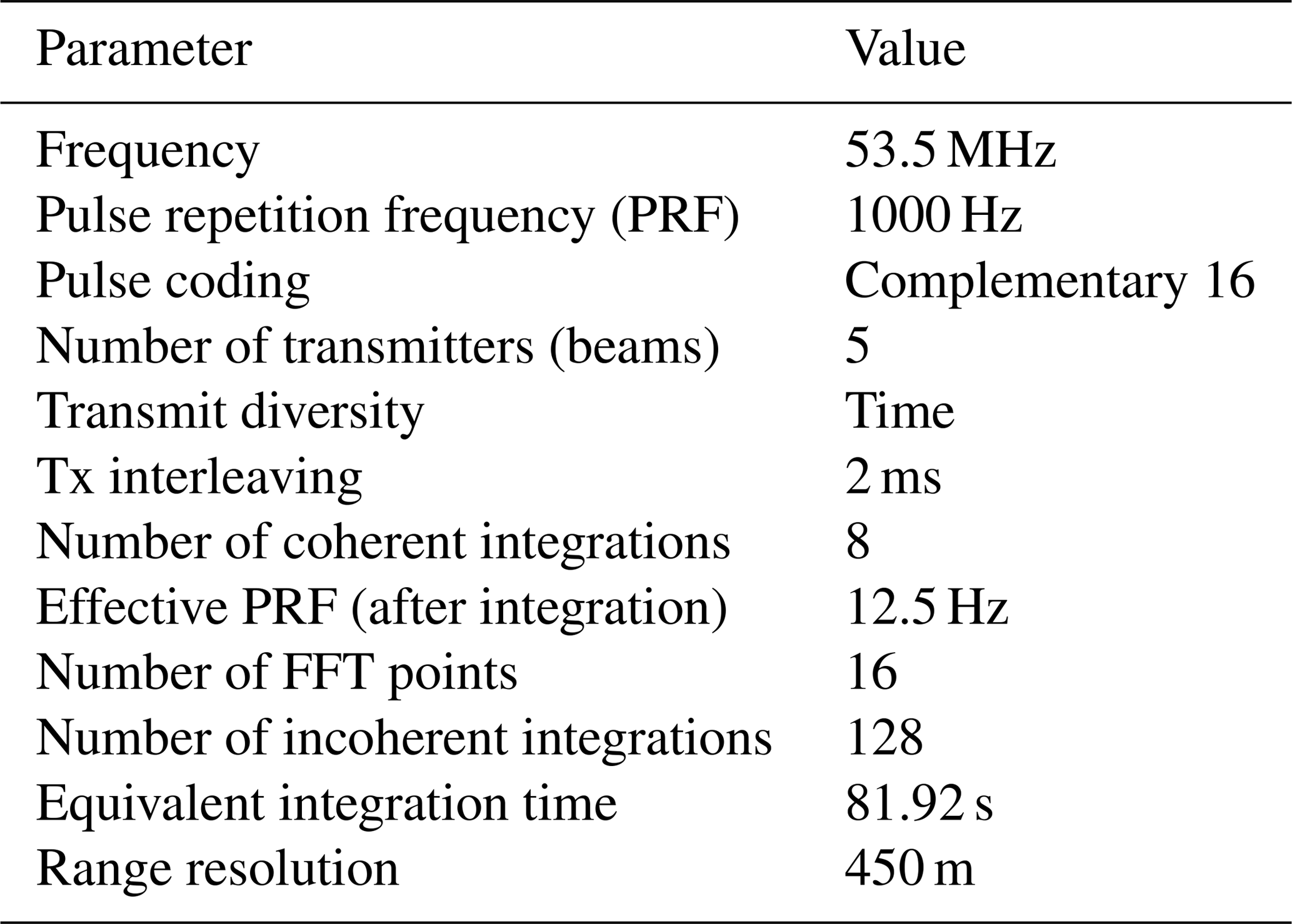
MAARSY is an active phased antenna array operating at 53 MHz, located in Andoya, Norway (69.30∘ N, 16.04∘ E). The array consists of 433 antenna elements, each with its own transceiver module that allow us to modulate the antennas in phase and amplitude independently. Using this capability, the transmitting or receiving beam can be steered in a desired direction up to 30∘ off zenith, with an angular resolution of 3.6∘ (e.g., Latteck et al., 2012a). In addition to its multibeam capability, MAARSY can be used for in-beam imaging experiments. In this case, the signals from a selected number of receiving antennas are stored, and later a digital beamforming algorithm (imaging) is applied to the data. Unlike the multibeam experiment, imaging allows a 2-D image to be obtained at once, avoiding the interleave from beam to beam. Currently, only 16 receivers are available at MAARSY. These 16 receive signals can be selected from groups of seven antennas, each called “hexagons”, or from a group of seven hexagons called “anemones” (see, e.g., Latteck et al., 2012b, for further technical details). For this campaign, we conducted an imaging experiment using 15 hexagons on reception similar to Sommer and Chau (2016)'s experiment. One receiver is always connected to the full antenna array and it is used as in the standard multiple experiments. The radar parameters of this experiment are summarized in Table 1.
2.2 MAARSY MIMO configuration
In order to improve the performance of our imaging experiment, we applied a coherent MIMO technique (Urco et al., 2018). The technique employs multiple independent transmitting antennas and multiple receiving antennas, both spatially separated, to take advantage of the transmit–receive geometry and to increase the angular resolution of the radar. If the antennas are closely separated or collocated, the signals from each transmitting–receiving path are coherent and can be combined to form a larger virtual receiving array. The resulting number of virtual receivers is equal to the number of transmitters times the number of receivers.
Depending on the transmitting and receiving antenna configuration, some virtual receivers can be redundant. In our experiment, we carefully selected the transmitting and receiving antenna configuration to get three special redundant virtual receivers. These three redundant virtual receivers were used for phase calibration of the transmitters as was done by Urco et al. (2018). Figure 1a shows the 15 hexagons used in reception and the three anemones used in transmission (B, D, F). Figure 1d shows the resulting virtual receiving antennas, whereby three of them are redundant and located at the origin.
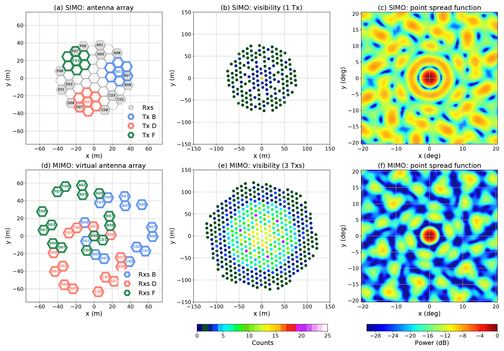
Figure 1MAARSY antenna configuration for SIMO (a, b, c) and MIMO (d, e, f). (a) 16 hexagons used in reception are shown in grey and three anemones used in transmission are colored. (b) Visibility samples for SIMO. (c) Point spread (or instrument) function for SIMO. (d) The virtual position of the resulting receiving antennas by using MIMO. (e) Visibility samples for MIMO. (f) Point spread (or instrument) function for MIMO. See text for further details.
In order to separate the contribution of each transmitter, a form of transmit diversity was needed. In Urco et al. (2018), three types of transmit diversity were proposed: code, time, and polarization. Code diversity is recommended for atmospheric observations given that this is not sensitive to the temporal correlation or polarization of the target of interest. Unfortunately, code diversity cannot be currently used in MAARSY. For targets for which the temporal correlation is less than the time separation between transmitters, time diversity can be applied. Given that PMSEs have a relative long correlation time (a few hundreds of milliseconds), we applied time diversity to enhance the spatiotemporal features of PMSE. The effective time separation between transmitters was 4, 4, and 8 ms between pairs BD, DF, and BF, respectively.
As explained by Urco et al. (2018), in a monostatic coherent MIMO radar, the relationship between the normalized spatial cross-correlation of signals from two different transmitting-receiving paths and the angular distribution of scattered power for a given range and frequency bin can be described by
where vm, p is the signal from the transmitting-receiving path (m,p), m being the receiver and p the transmitter; is the complex conjugate of the signal from the transmitting-receiving path (n,q), n being the receiver and q the transmitter; is the cross-correlation of two signals from antennas spatially separated; is the visibility sample at ; k is the wave number vector equal to (2π∕λ)θ. And λ is the radar wavelength; θ is the angle of arrival equal to which are the direction cosines in the (x, y, z) direction; B(θ) is the angular scattered power distribution, also known as brightness; Δrm, n is the spatial separation between receivers m and n; Δrp, q is the spatial separation between transmitters p and q; 2πfdτ is the phase difference due to the Doppler shift of the target, fd, where τ is the time separation between transmitters; ϕp, q is the phase difference between transmitters; ϕm, n is the phase difference between receivers.
A quick comparison between the visibility (sampling domain) for SIMO and MIMO, shown in Fig. 1b and e, indicates that the antenna aperture for MIMO is larger than the SIMO by ∼50 %. The difference lies in that the MIMO antenna aperture is defined as the maximum separation between two virtual receiving antennas, i.e., , whereas for SIMO, , and the antenna aperture is only defined by the maximum spatial separation between two receiving antennas. Figures 1c and f show the resulting instrument function or point spread function for SIMO and MIMO, respectively. As expected the half-power beamwidth (HPBW) for MIMO is ∼50 % smaller than for SIMO, resulting in an angular resolution of 2.4∘ for MIMO compared to 3.6∘ for SIMO. Furthermore, the sidelobes in the MIMO configuration are strongly reduced, given that the visibility is larger and contains no gaps.
Before inverting Eq. (1), the three phase differences due to time diversity (2πfdτ), to receivers (ϕm, n), and to transmitters (ϕp, q) need to be corrected. When the analysis is done in the frequency domain we can easily correct the value 2πfdτ, given that we know the frequency and the time separation between transmitters. On the other hand, the phase offsets between receivers have been calibrated using Cassiopeia A as a radio source (e.g., Chau et al., 2014). Additionally, we have calibrated the phase offset between transmitters using the three redundant virtual receivers described above. Each of the redundant virtual receivers comes from one transmitter. They were compared to have zero phase difference between each other, given that the three of them must be located in the same virtual position (see, e.g., Urco et al., 2018, for more details).
Once the imaging system is calibrated we can invert Eq. (1) to obtain the estimated brightness . Given that the number of unique visibility samples is still less than the number of unknowns (brightness points), some kind of regularization is needed to solve Eq. (1). Two of the most well-known radar imaging techniques applied to atmospheric and ionospheric targets are Capon (Palmer et al., 1998) and MaxEnt (Hysell, 1996).
3.1 Capon technique
As described by Kudeki and Sürücü (1991), the angular resolution obtained from a direct inversion of Eq. (1) using the inverse Fourier transform is limited by the longest baseline and the unmeasured antenna separations (visibility gaps). Palmer et al. (1998) proposed a new technique to improve the angular resolution based on the work of Capon (1969). Capon can be seen as an extension of the inverse Fourier transform. The difference lies in the fact that Capon chooses the antenna weights adaptively in order to minimize the sidelobe interference from signals outside of the direction of interest according to the data. Capon's technique provides an estimate of the brightness function given by
where
is the Fourier kernel and is the visibility due to the virtual receivers and , with i and j being the receiver indices and l and k being the transmitter indices.
3.2 Maximum entropy technique
Even when MIMO is used, the problem is still underdetermined. Thus, there are infinite possible image solutions, B, which agree with the data, V. Of all possibilities, MaxEnt chooses the solution with the maximum entropy or minimal information content (e.g., Hysell, 1996) as the one to be the most likely brightness distribution and the most consistent with the available visibility data and their statistical uncertainties. The entropy for a given frequency bin and range can be defined as
where F is the summation of the brightness distribution over the region of interest. The solution of Eq. (1) is defined by
where ϵ is the noise amplitude associated with the visibility measurements. In this work, we have also considered the improvements of Hysell and Chau (2006). Specifically, we have taken into account the transmitting beam pattern and the statistical uncertainties of all the visibility pairs.
Figure 2 shows the resulting 24-bit range–time Doppler intensity (RTDI) image of the vertical beam for 32 h of continuous operation on 16 and 17 July 2017. This plot was obtained after applying MaxEnt to the data and selecting the values that belong to the zenith angle. The signal intensity is represented as lightness, Doppler information as hue, and spectral width as saturation. As shown later, the resulting HPBW for this experiment is <1∘, indicating that the Doppler information must be mainly due to the vertical motion. The RTDI plot indicates that the vertical motion is slow (green color) as expected. Nevertheless, there are two regions at 23:30 and 06:30 LT around 89 km in which the Doppler velocity presents unrealistic values. Indeed, PMSE were too strong at that time, so even the antenna sidelobes can be seen. Unfortunately, the imaging algorithm cannot assign the correct angle of arrival to these unusually strong echoes due to the angular ambiguity associated with our antenna array. The angular ambiguity is defined by the minimum separation between two antennas. The smaller the separation, the larger the angle without ambiguity (e.g., Woodman, 1997). A manual angular correction can be applied knowing the Doppler but it is a hard task in the presence of many targets. A smaller baseline is recommended in future experiments for these special cases.
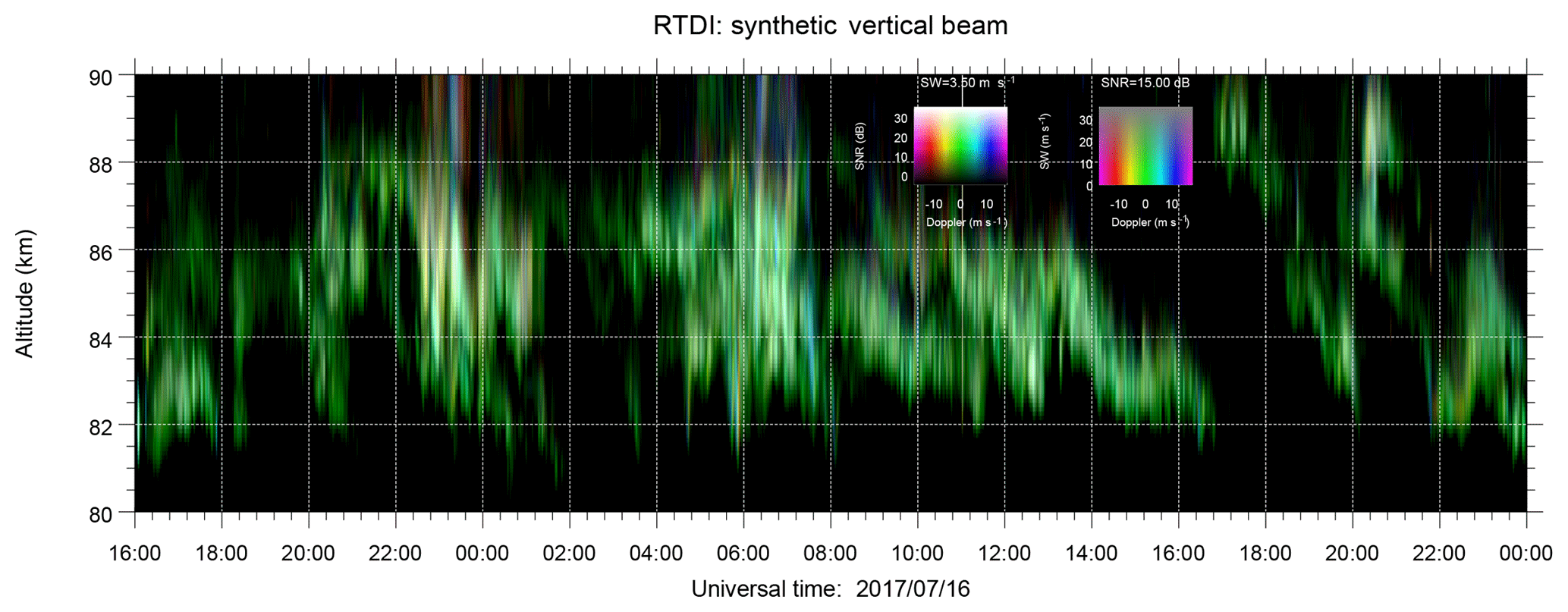
Figure 2A 24-bit image of a range–time Doppler intensity (RTDI) plot of PMSEs using MIMO, with time diversity conducted on 16 and 17 July 2017. The signal intensity is represented as lightness, Doppler information as hue, and spectral width as saturation. The legend on the left represents the SNR vs. Doppler color map for a saturation of 90 %. The legend on the right represents the spectral width vs. Doppler for a lightness of 50 %. Note that only the signal corresponding to the narrow region in the illuminated area is shown.
4.1 SIMO vs. MIMO results
Since the estimated brightness is expressed in polar coordinates , a cubic spline interpolation was applied to convert them to Cartesian coordinates, to , with the radar being located at the center (x=0, y=0, z=0). Below we show the results of two selected events (Events 1 and 2) after performing such interpolation. For both events, we show x vs. y cuts for a given z, as well as x vs. z cuts for a given y, where x, y, and z represent the east–west (EW) direction, north–south direction (NS), and altitude, respectively.
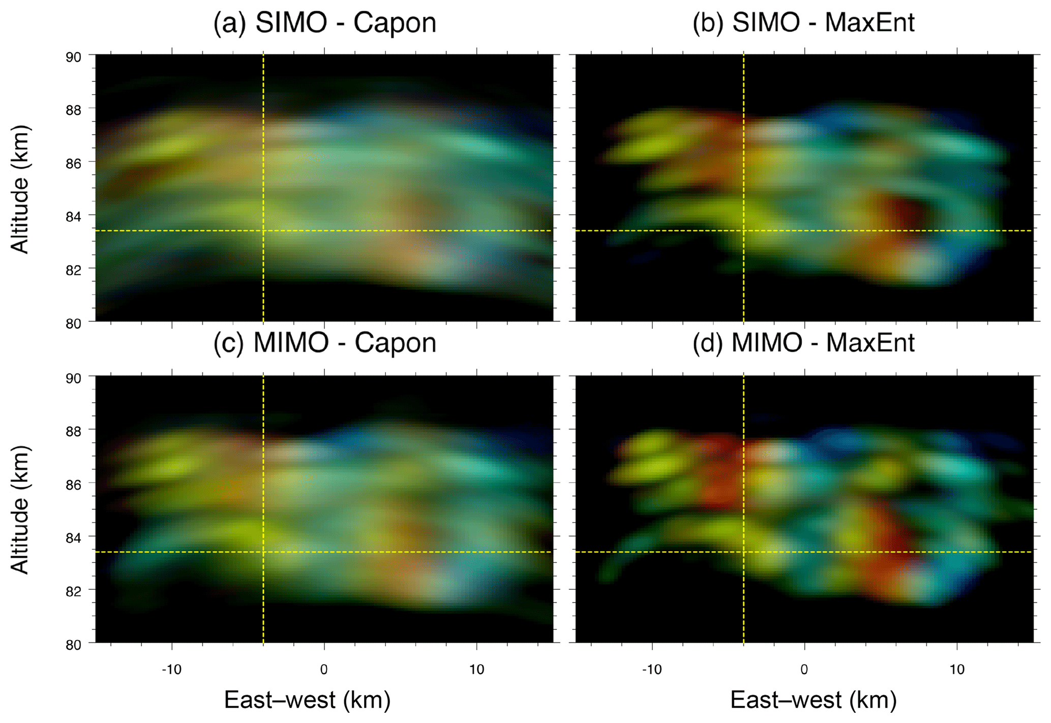
Examples of EW–NS and EW–altitude 2-D images for Event 1 obtained by applying Capon and MaxEnt to two different antenna configurations, SIMO and MIMO, are shown in Figs. 3 and 4, respectively. Four different results are shown: (a) SIMO-Capon, (b) SIMO-MaxEnt, (c) MIMO-Capon, and (d) MIMO-MaxEnt. Having a quick look at the results, it is clearly observable that (1) MaxEnt outperforms Capon when the same antenna configuration is used, either SIMO or MIMO. This was already pointed out by previous works (e.g., Yu et al., 2000; Harding and Milla, 2013). (2) As expected, MIMO shows a cleaner and more defined image compared to SIMO, when either Capon or MaxEnt is employed. (3) The improvement of using MIMO instead of SIMO is much better in MaxEnt than Capon. The improvement of MIMO-Capon with respect to SIMO-Capon is about 50 % due to the larger virtual antenna array, whereas the improvement of MIMO-MaxEnt with respect to SIMO-MaxEnt is much better than 50 %. This difference lies in the fact that Capon tries to reduce the sidelobes, adaptively steering them to echo-free zones. Unfortunately, for the two events shown, most of the illuminated area is filled with PMSE scattering, and thus the performance of Capon is expected to be comparable to the conventional beamforming (inverse Fourier transform). In the case of MaxEnt, the improvement is mainly due to the larger virtual antenna array and the use of statistical uncertainties as described by Hysell and Chau (2006). Unlike Capon, our MaxEnt implementation takes advantage of the redundant visibility pairs, giving more weight to pairs with less uncertainty, i.e. more redundancy. Figure 1b and e show the visibility pairs and their redundancy for SIMO and MIMO, respectively.

Figure 3EW–NS images for z=85.8 km obtained from applying four different implementations, (a) SIMO-Capon, (b) SIMO-MaxEnt, (c) MIMO-Capon, and (d) MIMO-MaxEnt, at 00:56:55 UT on 17 July 2017, i.e., Event 1. Images are color coded the same as in Fig. 2. The yellow dashed horizontal and vertical lines represent the location of the NS–EW cuts shown in later figures for Event 1.
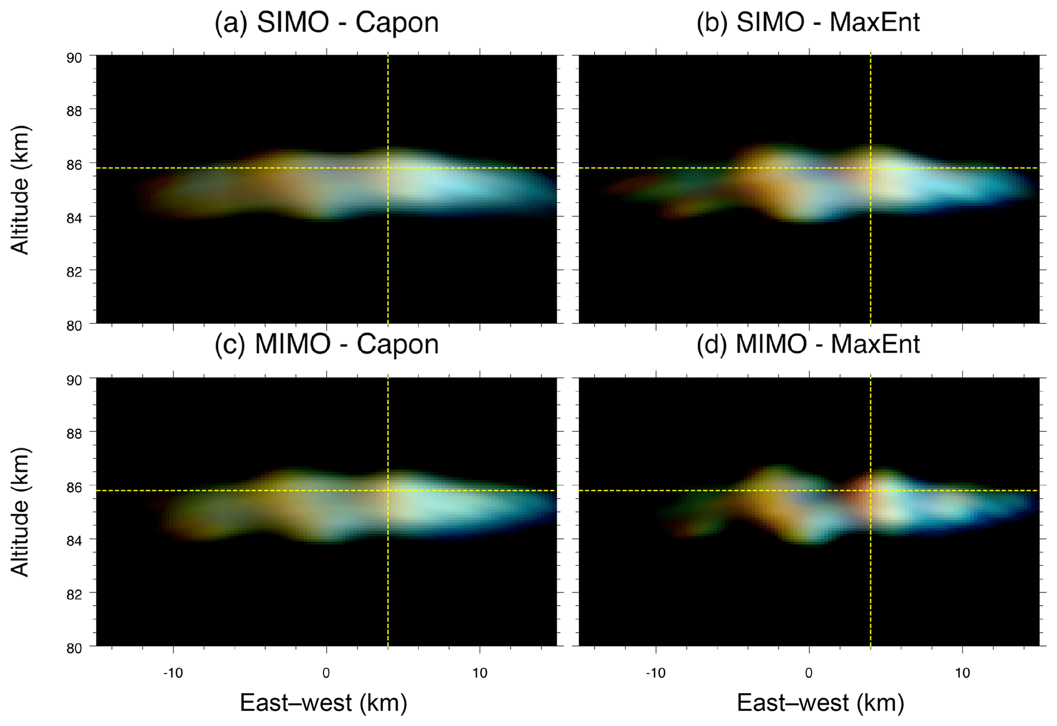
Figure 4Similar to Fig. 3, but for an EW–altitude cut at y=0 km. The yellow dashed horizontal lines represent the location of the altitude cuts shown in previous and later figures for Event 1.
Coming back to our comparison of SIMO vs. MIMO, with MIMO-MaxEnt, small wave-like structures of 2 km wavelength can be clearly observed, which are invisible in SIMO implementations or MIMO-Capon. For example, observe the two wavefronts at x=10 km in Fig. 3d, right beside the larger meridionally oriented wavefronts of 7 km wavelength. This indicates that wave-like structures of different wavelengths coexist within PMSEs as previously seen in NLCs (e.g., Baumgarten and Fritts, 2014). In addition, Fig. 4d shows that the ascending structures (red color) have a higher signal-to-noise ratio (SNR) than the descending structures (blue color).
We show similar 2-D cuts for Event 2 in Figs. 5 and 6 for z=82.7 km and km, respectively. In this case, the observed wavelength is 12 km. Unlike the first event, the SNR is similar for targets with negative and positive Doppler. Figure 6d shows two very interesting points: (a) a very well-defined wave-like structure between 82 and 84 km and (b) a quasi-uniform structure between 84 and 86 km, which apparently has been modulated by the first wave. In this case, the wave-like structure is easily discernible even with SIMO-Capon, given that the wavelengths are larger than in Event 1 (see Fig. 5a).

Figure 5Same as Fig. 3 but at 05:56:13 UT on 17 July 2017, i.e., Event 2. The yellow dashed horizontal and vertical lines represent the location of the NS/EW cuts shown in later figures for Event 2.
4.2 MIMO results
Having shown the better qualitative performance of MIMO-MaxEnt with respect to the other three implementations for the two selected events above, next we present extended results using just MIMO-MaxEnt.
Figure 7 shows the evolution in time of two selected events, i.e., Event 1 (panels a, b, and c), and Event 2 (panels d, e, and f). Figure 7a and d show the time evolution vs. altitude for selected EW and NS coordinates. In these plots, we can appreciate how variable PMSE structures are, showing different altitudinal extensions. Note that the effective horizontal area is less than 1 km2 in both cases.
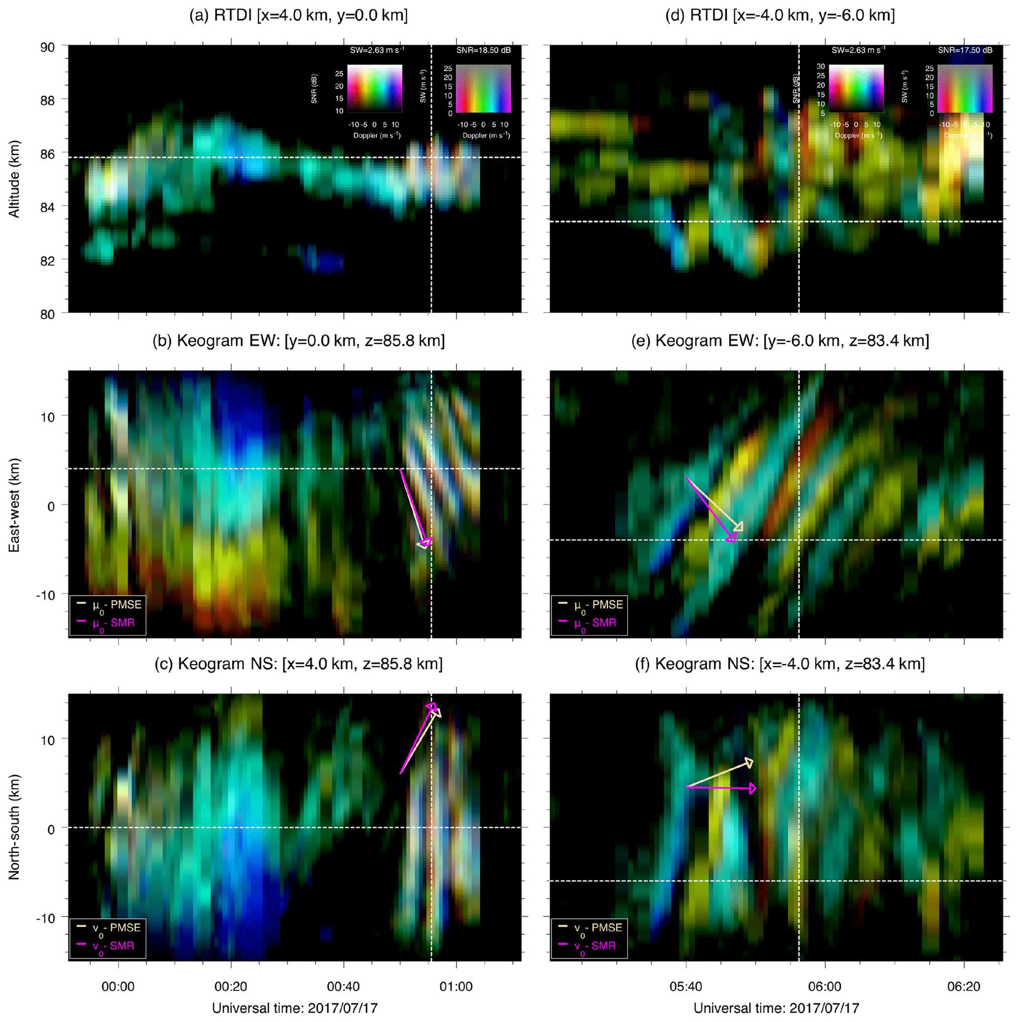
Figure 724-bit time representation images of PMSE structures as a function of altitude (RTDI) (a, d), EW location (keogram) (b, e), and NS location (keogram) (c, f) for selected cuts, for both Event 1 (a, b, c) and Event 2 (d, e, f). In the keograms, the wind components obtained with specular meteor radars (SMRs) and MAARSY PMSEs are shown by pink and yellow arrows, respectively. The white dashed horizontal lines represent the location of the altitude, EW and NS cuts shown in previous figures, and current keograms for Events 1 and 2. The white dashed vertical lines represent the time of the cuts shown in previous figures.
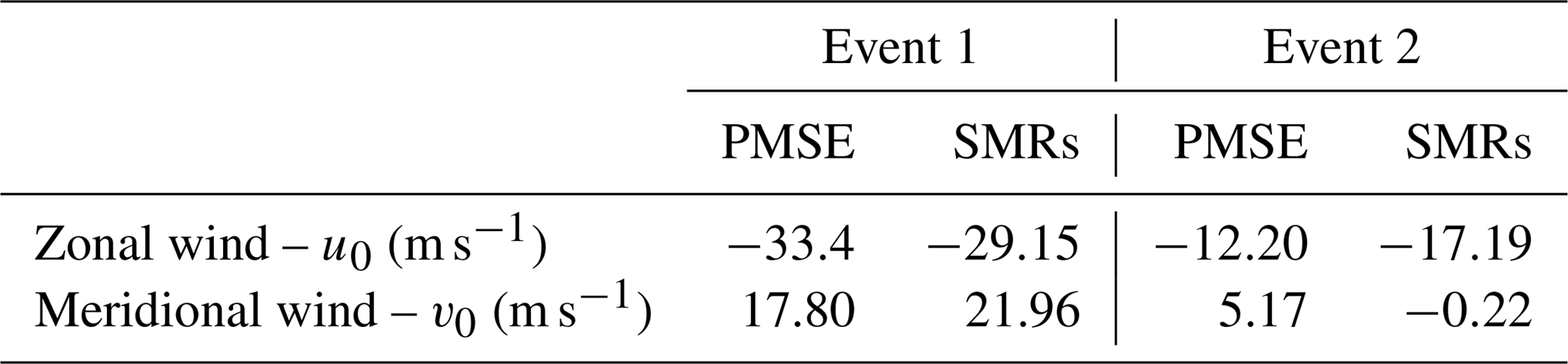
The second and third row of Fig. 7 show the time evolution vs. EW direction and the time evolution vs. NS direction, for EW and NS keograms, respectively. We have included the zonal (u0) and meridional (v0) wind velocity estimated from combining a couple of specular meteor radars (SMRs) (pink arrow) and from MAARSY based on PMSE Doppler velocities (yellow arrow). The wind values are shown in Table 3. Since this is a “time” vs. “distance” plot, the zonal and meridional wind are represented by arrows for which their slopes indicate the wind magnitude, i.e, how long a target is displaced in the y axis for a certain time in the x axis. The SMR winds were obtained from combining SMR detections from Andenes and Tromsø in northern Norway (see, e.g., Chau et al., 2017, for details). In order to estimate the winds from PMSEs we used the following formula:
where vrad is the radial wind, are the direction cosines, and (u, v, w) are the zonal, meridional, and vertical wind direction, respectively. Assuming a constant u, v, and w for a given altitude bin and time bin, and taking all the measurements with a SNR higher than −5 dB, we invert Eq. (7) and get u0, v0, and w0, mean values of u, v, and w respectively.
The keograms for Event 1, i.e., from 00:50 to 01:05 UTC, show that the meridionally oriented wavefronts have a limited vertical extent centered at 85 km (Fig. 7a), and since this wave has a finite wavelength in the EW direction, the zonal wave propagation can clearly be observed in Fig. 7b, which shows that the elongated meridionally oriented wavefronts are zonally drifting with the same direction and with the same speed as the wind. In the NS direction, the meridional drifting of the wave is not clearly observed due to the elongated structure. Mesospheric wave-like features observed with airglow imagers (ripples) have also been noticed to drift with the background wind (e.g., Hecht, 2003). These ripples have been associated with gravity wave breaking and are a clear signature of atmospheric instability.
Figure 7d shows another interesting wave-like example (Event 2). Unlike the first case, this wave does not keep its amplitude in the vertical direction; see Fig. 7d. It grows and then disappears. Its direction of propagation in the zonal and meridional direction is also interesting. As shown in Fig. 7e, the direction of propagation in the zonal direction is completely opposite to the background wind. Whereas the wind is going from east to west, the wave propagates from west to east. In the NS direction (Fig. 7f), the wind is close to zero and we do not expect changes in this direction. Since its wavelength is relatively small, this structure might be classified as an instability; however, the opposite direction of propagation suggests that it could be a propagating gravity wave. Further investigation of these events is needed to understand the physical mechanisms behind them, including lidar and airglow imager observations.
PMSEs have been used as a neutral wind tracer, assuming that u, v, and w are constant and homogeneous during the analyzed time (e.g., Balsley and Riddle, 1984; Fritts et al., 1990; Hoppe and Fritts, 1995; Stober et al., 2013). Therefore, those works assumed that scatters from PMSEs are moving with the neutral wind at the same velocity and in the same direction. Unlike winds obtained from SMR, winds from PMSEs are affected by local disturbances, as shown in Fig. 7e and f. When the dynamics of local structures are not in agreement with the wind dynamics, a bias could be introduced in the wind estimation (as shown in the Event 2). However, when these local disturbances are moving with the wind, the estimated wind is not affected (Event 1). Note that the PMSE winds are in good agreement with the SMR winds in Event 1, but they are not for Event 2, particularly for the meridional component.
An animated sequence of the two events has been included in the Video supplement, i.e., Movies S1 and S2. For both events, the sequence includes selected cuts of EW–NS, EW–altitude, and NS–altitude. In Movie S1, we identify at least four examples of monochromatic waves with different wavelengths drifting with the wind in the northwest direction (at 23:57:37, 00:02:24, 00:10:57, and 00:55:33 UTC). Interestingly, in this case, longitudinal and transverse waves both drift with the background wind. In Movie S2, we show the complete evolution in time of Event 2. In the EW–altitude cut, the wave structure between 82 and 85 km drifts against the wind, whereas a layer at 87 km between 05:20 and 05:30 UTC follows the background wind. Note the projected radial wind (from red to blue) indicates a westward wind. These events are good examples of the complicated dynamics within PMSEs. Further analysis and interpretation of these high-resolution spatiotemporal structures will be done in a future work.
Figures 8 and 9 show 3-D maps of (a) the signal-to-noise ratio (SNR), (b) radial velocity, (c) locally enhanced SNR, and (d) residual radial velocity (i.e., vres), for Events 1 and 2, respectively. In addition contours of locally enhanced SNR are overplotted on both the radial velocities. The SNR and radial velocity were obtained from the first and second spectral moments (e.g., Doviak and Zrnić, 1993). The locally enhanced SNR has been obtained using a 2-D Gaussian function kernel with a width of 6 pixels. The local enhancements allow us to observe weak structures within the strong one. For example, wave fronts are distinguishable in Fig. 8c which were not visible in Fig. 8a. On the other hand, the residual radial velocity was estimated by removing the contributions of the estimated mean horizontal velocities in the measured radial velocities; i.e.,
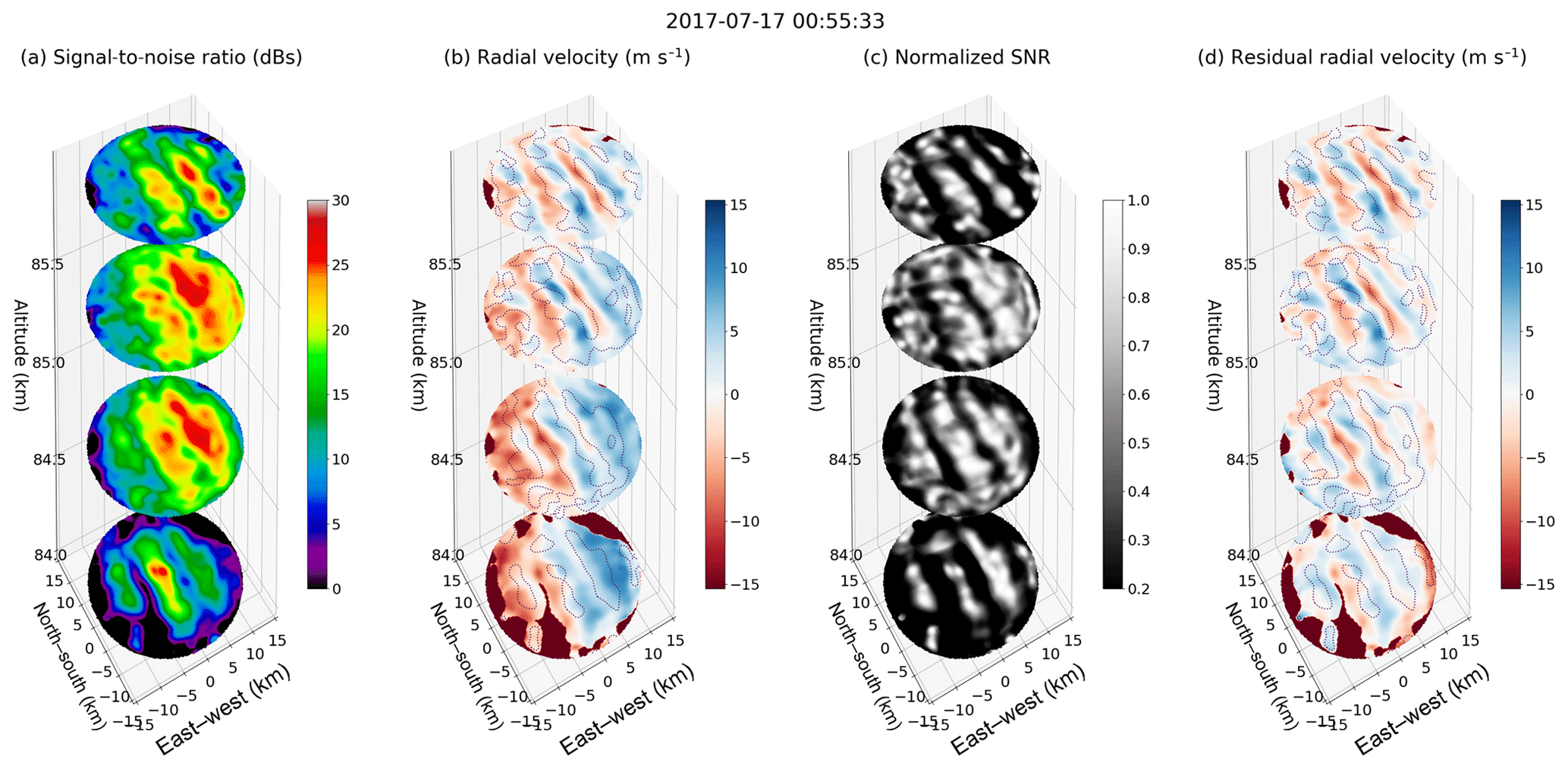
Figure 8The 3-D contour plots at 00:55:33 UT on 17 July 2017, i.e., Event 1, for four selected altitudes: 84, 84.6, 85.2, and 85.8 km. The following are shown for each altitude: (a) SNR, (b) radial velocity, (c) locally enhanced SNR, and (d) residual radial velocity. Contours on locally enhanced SNR are overplotted in both velocity plots.
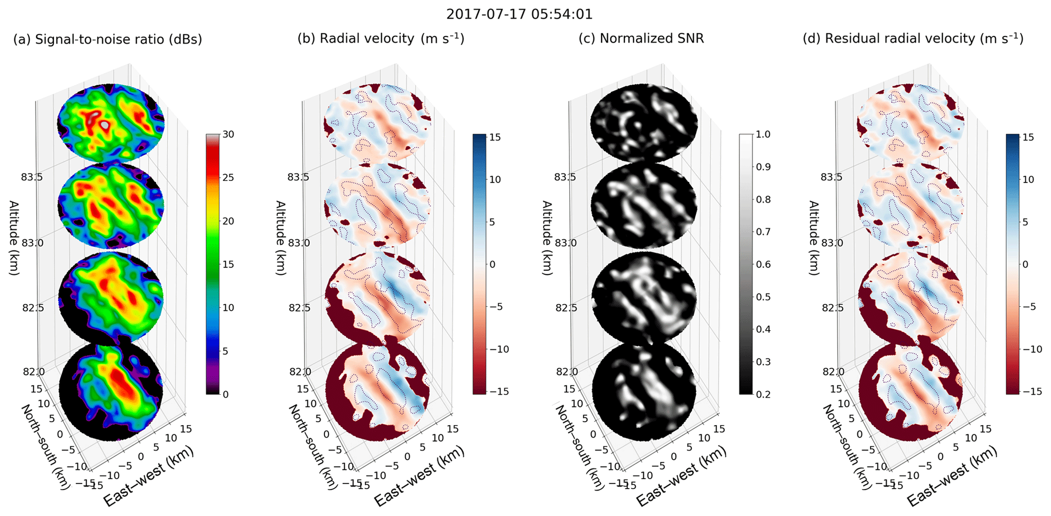
Figure 9Same as Fig 8, but at 05:54:01 UT on 17 July 2017 for altitudes 82, 82.7, 83.4, and 84 km., i.e., Event 2.
Assuming that the vres is mainly due to the vertical motion, we can clearly see in Fig. 8d how up (red) and down (blue) structures drift across the illuminated area, maybe due to KHI. Similarly, Fig. 9 shows animated images of Event 2. In this case, the horizontal wind was small and most of the radial velocity was due to the vertical motion; i.e., radial velocity and residual velocities are almost the same. As mentioned above, in this event, the waves propagate horizontally against the weak horizontal wind.
The animated versions of Figs. 8 and 9 are shown in Movies S3 and S4, respectively. Although the information might be redundant when compared to Movies S1 and S2, we have decided to include them to provide a more standard view of typical spectral parameters of a multibeam radar.
Making a quantitative comparison between SIMO and MIMO for real targets is not an easy task. We need a prior knowledge of the brightness to make a good analysis. This is not the case for PMSE. Fortunately, our observations include echoes from specular meteors; see the bright echoes located at (−10.5, −12.5) in Fig. 3d. Indeed, meteor echoes can be observed in the PMSE region, but the great majority of them occur outside this window. When a meteor echo occurs in the PMSE altitude it will be short-lived (less than a few hundred milliseconds). In previous studies meteor echoes were treated as outliers and were removed from the measurements (e.g., Hashimoto et al., 2014). For our benefit they can also be used to evaluate the angular resolution that can be achieved with our implementations quantitatively. A specular meteor echo could be considered to be a point target. Along with its trajectory, the trail is long (hundreds of meters to a few kilometers), but its angular response is narrow. In the transverse direction to the trail, it is very narrow and its angular response is also narrow.
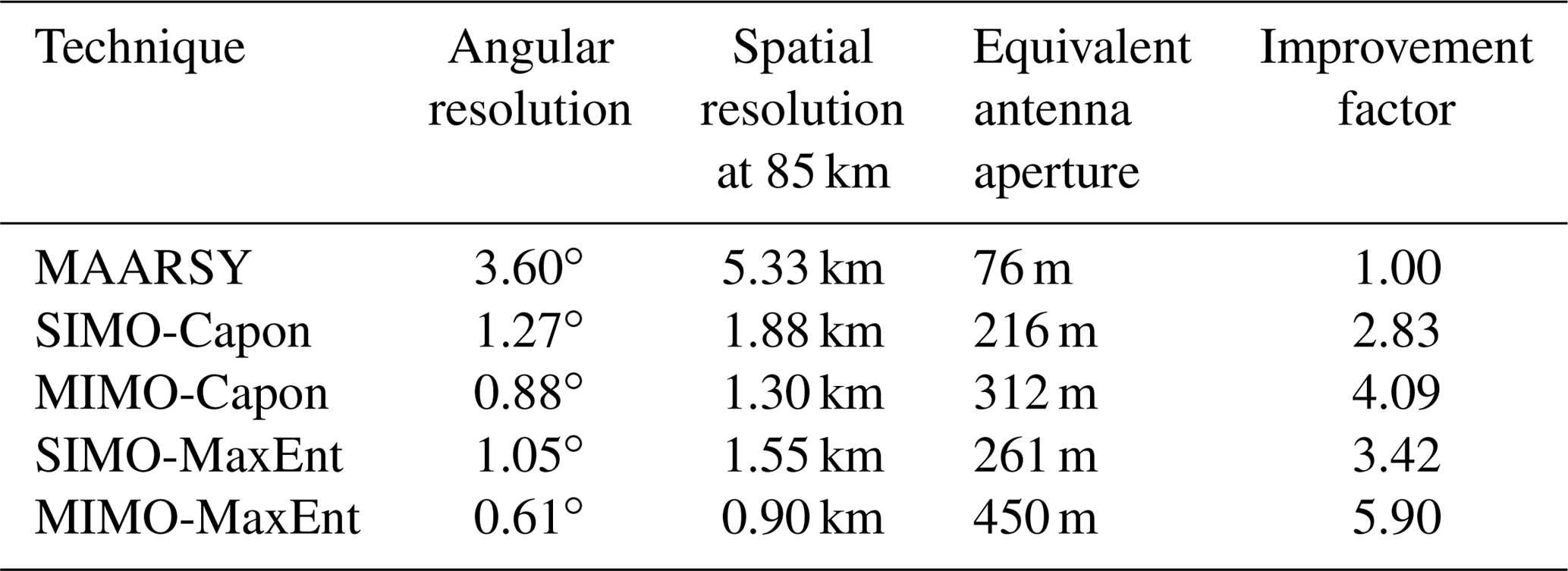
In Fig. 10 we show the normalized angular scattered power distribution for a specular meteor using SIMO and MIMO in combination with Capon and MaxEnt. As expected, the range resolution does not change for SIMO or MIMO (see Fig. 10a). We see a peak at 89.1 km and low power at other ranges. However, when comparing Capon and MaxEnt, MaxEnt shows us a clean power distribution along all the ranges, while Capon shows us a remaining sidelobe contamination in other ranges, coming from other angles. This indicates that, even with MIMO, Capon does not suppress the sidelobes as well as MaxEnt. Figure 10b and c show us the angular power distribution for θx and θy, respectively, for which the points are the samples for a given angle and the continuous line is a fitted Gaussian function. Using the fitted function, we estimated the half-power beamwidth (HPBW) for each implementation. Table 2 summarizes the angular resolution and the improvement factor for each method compared to the theoretical angular resolution of the full array MAARSY radar. As we expected the improvement between SIMO and MIMO is about 1.5, given that we increased the antenna aperture for MIMO by ∼50 %. When combining MIMO and MaxEnt, surprisingly, we got an angular resolution of ∼0.6∘, i.e., more than 5 times better than MAARSY's HPBW.
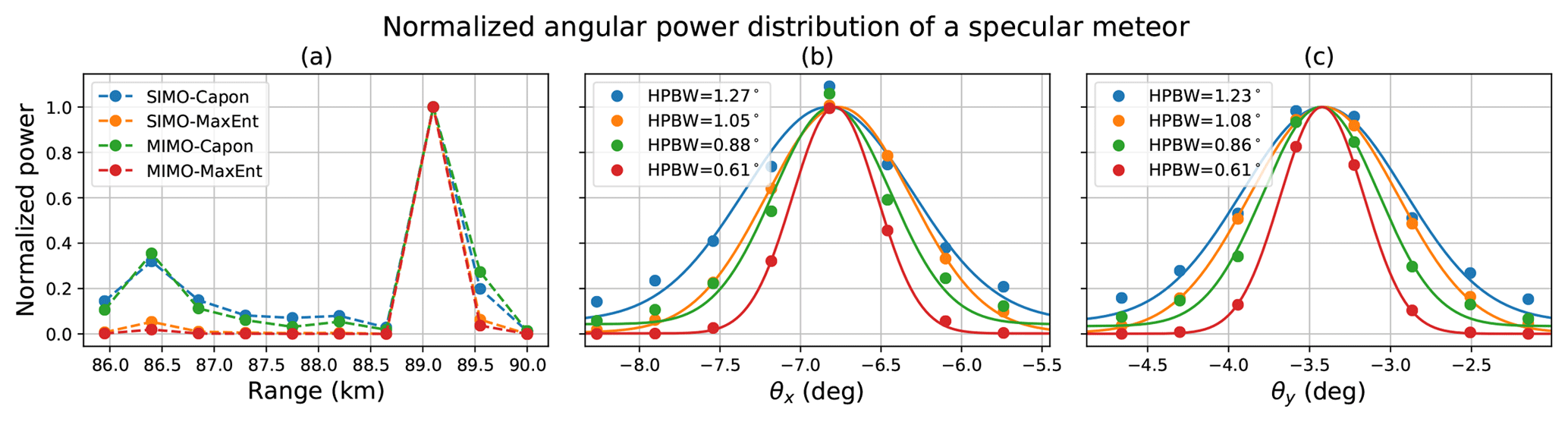
Figure 10Normalized angular power distribution of a specular meteor echo as a function of (a) range, (b) EW angle (θx), and NS angle (θy). The results are shown for all four implementations, i.e., SIMO-Capon (blue), SIMO-MaxEnt (orange), MIMO-Capon (green), and MIMO-MaxEnt (red).
We have shown qualitatively and quantitatively that radar imaging of PMSEs is significantly improved when using MIMO instead of SIMO configurations, by at least 50 %. Two different imaging methods have been applied, Capon and MaxEnt. As expected from previous works, MaxEnt images are better than Capon images; however, MaxEnt is computationally more demanding. Similarly, we found that the quality of MIMO-Capon is comparable to SIMO-MaxEnt.
Even though MIMO allows us to improve the point spread function, it is not perfect. We expect some artifacts due to the sidelobes which are −15 dB weaker than the main lobe; see Fig. 1f. When strong and weak echoes coexist in the same region, some artifacts might be confused as weak echoes. Although Capon and MaxEnt help to minimize the sidelobe contribution, we are being conservative by employing a relatively large SNR threshold (>5 dB), i.e., discarding weak echoes which might be contaminated by strong sidelobe echoes. By doing this we are increasing the statistical significance of our results which are persistent in time and space, as shown in the animations and the keograms.
The preliminary results using MIMO-MaxEnt are allowing us to observe PMSEs with unprecedented horizontal resolution (<1 km) compared to multibeam scanning experiments (Stober et al., 2013), and therefore the identification of structures with horizontal wavelengths less than 10 km (e.g., Event 1 above). For structures with wavelengths of the order of 15–20 km or so, the other imaging implementations, i.e., SIMO-Capon, SIMO-MaxEnt, and MIMO-Capon, are sufficiently good to characterize them. These new capabilities will allow KHIs and general GWs (not only monochromatic) to be better identified and characterized than previously done at polar mesospheric heights during the summer. Our proposed technique complements previous observations that have been performed at nighttime when the sky is clear using airglows and lidars (e.g., Smith, 2013; Hecht et al., 2000, 2007; Taylor et al., 2007).
We will leave the detailed analysis and interpretation of these events and other events observed with this new capability for a future effort. In the following paragraphs, we discuss the technical results and propose future improvements.
The improved resolution using MIMO results from the larger effective visibility aperture and the larger number of independent samples, as compared to a SIMO configuration, i.e., 125 m instead of 76 m and 475 samples instead of 163 samples, respectively. In addition, the MaxEnt approach allows an improvement at least a factor of 2 in angular resolution compared to Capon. The maximum number of horizontal blobs that could theoretically be estimated for each range, time, and “color” (i.e., frequency bin) would be 79 (), whereby each blob is characterized by a 2-D Gaussian function with six parameters (e.g., Chau and Woodman, 2001). Another reason for the better results using MIMO-MaxEnt is the number of redundant visibility measurements. Although they do not provide additional information in terms of degrees of freedom, the redundancy helps to reduce the statistical uncertainties of such visibility samples. Recall in our MIMO implementation that there are 1980 visibility samples (45×44), and only 475 are independent.
Despite the significant improvement, not everything is positive about applying MIMO. In the following paragraphs, we discussed the critical points of applying MIMO in terms of (a) power-aperture reduction and (b) computational demands and real-time applicability.
As indicated by Urco et al. (2018), in atmospheric radars MIMO is applicable to targets with a large RCS, since a reduction of power aperture is inherent to MIMO. In our particular application to PMSEs, the transmitter sections were 1∕7 of the total area, and therefore also 1∕7 of the total transmitter power, i.e., −17 dB transmitting signal, of usual experiments. In reception, 15 groups of seven antennas (hexagons) were used instead of the 433 available antennas. Moreover, given the time multiplexing, the number of coherent integrations was reduced and therefore the noise was increased, when compared to standard operations. In total, the sensitivity of our MIMO experiment is 27 dB lower. Looking at the PMSE RCS in Fig. 2 of Latteck and Strelnikova (2015), our MIMO observations are limited to PMSEs with RCS larger than 10−14 m−1, i.e., approximately 40 % of the usual seasonal MAARSY PMSE observations.
MaxEnt is known to be computationally more demanding than Capon in SIMO applications (e.g., Yu et al., 2000). In the case of MIMO, the computational demands are significantly increased, given the larger number of effective receivers, i.e., 45 instead of 15. In terms of visibility pairs, the increase is from 210 to 1980. In the case of Capon, real-time processing is still possible with these increased numbers of samples; however, MaxEnt for both SIMO and MIMO is not applicable in a real-time application. For example, for 80 s of data using an i5 PC with 15 cores, the processing times are 20 min and 3 h for SIMO-MaxEnt and MIMO-MaxEnt, respectively. A future improvement to make MIMO-MaxEnt faster would be to use only one value of each redundant visibility sample, i.e., to only work with 475 independent samples instead of all 1980 measured visibility samples. Such a value could be obtained either from the average of all the values sampling the same visibility or by preselecting only one of them. After all, many of the independent samples are obtained with only one sample (green dots in Fig. 1e).
In general, a critical point for PMSE imaging is the drifting nature of the echoes. PMSE correlation times are relatively short, and under stationary conditions, one would require a few minutes of incoherent integration to reduce the statistical uncertainties of the visibility estimates. However, the structures to be imaged might move between 2 and 5 km in 60 s for typical mesospheric motions (40–80 m s−1), either from drifting with the background wind (Event 1) or from wave propagation (Event 2). These drifting structures limit further the angular resolution that can be accomplished by any method since the resulting image will be significantly blurred for integration times of a few minutes.
To deal with the drifting nature of PMSEs, in future studies we will explore tracking techniques, i.e., make use of this information to improve the angular resolution (e.g., Vaswani and Zhan, 2016). Given the computational demands of MaxEnt in particular when combined with MIMO, we will also explore radar imaging with compressed sensing (CS) techniques (e.g., Donoho, 2006; Candes and Wakin, 2008). Harding and Milla (2013) applied CS to Jicamarca F-region irregularities, and show that CS produces results similar to MaxEnt. Our plan is to use MIMO-MaxEnt as a reference for other radar imaging techniques using SIMO, for example, CS in combination with tracking. Besides the computational demands, MIMO might not be applicable at other atmospheric radar sites, and therefore the exploration of other techniques using SIMO is required.
An additional improvement to the current observations would be the use of shorter pulses and therefore better range resolution, for example, 150 m. Further improvement in range could also be accomplished by applying range imaging (e.g., Palmer et al., 1998; Yu and Palmer, 2001), particularly in combination with the radar imaging implementations of this work, allowing angular resolutions less than 1∘.
In this work, we have successfully implemented coherent MIMO with radar imaging at MAARSY to observe PMSEs with unprecedented angular resolution. The obtained resolution results from the combination of a larger effective aperture, a higher number of independent visibility samples resulting from MIMO, and improved angular resolution resulting from MaxEnt. Quantitatively, the maximum angular resolution accomplished is ∼0.6∘, which is equivalent to having a 450 m diameter visibility aperture at 53.5 MHz and is a significant improvement to the MAARSY standard angular resolution of 3.6∘.
The preliminary results with MIMO-MaxEnt allowed us to clearly identify structures slightly less than 1 km in diameter and wave-like structures with horizontal wavelengths less than 10 km, with a time resolution around 60 s. The identification of such structures, with varying degrees of intensity, suggests that one has to be careful about using PMSEs for estimating the background wind assuming horizontal homogeneity. Not only is the vertical wind not homogeneous, but also the brightness is not homogeneous horizontally.
Given the relatively long temporal correlation of PMSEs, i.e., a few minutes, larger integration of the noisy visibility in time would allow fewer statistical uncertainties in the resulting images of the two events presented. However, PMSE structures drift as they are imaged; therefore long integration times result in angular smearing. In the future, we plan to use the drifting information to improve the angular resolution by applying tracking techniques.
As mentioned above, the implementation of MIMO-MaxEnt is computationally intensive and is currently not applicable to real-time processing. On the other hand, MIMO-Capon can be implemented in real-time processing. Our strategy for near-future observations would be to use MIMO-Capon for real-time processing and use MIMO-MaxEnt for special events until more efficient implementations and/or faster computers are available.
Our MIMO-MaxEnt results for the two events presented here, namely the PMSE power amplitude as a function of EW, NS, altitude, and time, are shared at ftp://ftp.iap-kborn.de/data-in-publications/UrcoAMT2018b.
An image sequence for the two events presented in this work has been added as a supplement. These sequences show the time evolution of PMSE structures for selected EW, NS, and altitude cuts. An example of wave structures drifting with and against the wind is showed in Movies S1 and S2, respectively.
JMU and JLC conceived the idea. JLC, TW, and JMU discussed the theoretical framework. JLC, JMU, and RL designed the experiment. RL and JMU carried out the experiment. JMU processed the experimental data and performed the analysis. JLC contributed to the interpretation of the results. JMU wrote the manuscript with support from JLC. All authors provided critical feedback and helped to improve the manuscript.
The authors declare that they have no conflict of interest.
This article is part of the special issue “Layered phenomena in the mesopause region (ACP/AMT inter-journal SI)”. It is a result of the LPMR workshop 2017 (LPMR-2017), Kühlungsborn, Germany, 18–22 September 2017.
We would like to thank Toralf Renkwitz for providing the receivers' phase
offsets and Marius Zecha for MAARSY data handling. This work was partially
supported by the Deutsche Forschunggemeinschaft (DFG, German Research
Foundation) under SPP 1788 (CoSIP)-CH1482/3-1 and by the WATILA Project
(SAW-2015-IAP-1).
The publication of this article was funded by the
Open Access
Fund of the Leibniz Association.
Edited by: William Ward
Reviewed by: Jia Yue and Ian McCrea
Balsley, B. B. and Riddle, A. C.: Monthly mean values of the mesospheric wind field over Poker Flat, Alaska, J. Atmos. Sci., 41, 2368–2375, 1984. a
Baumgarten, G. and Fritts, D. C.: Quantifying Kelvin-Helmholtz instability dynamics observed in noctilucent clouds: 1. Methods and observations, J. Geophys. Res.-Atmos., 119, 9324–9337, https://doi.org/10.1002/2014JD021832, 2014. a, b
Candes, E. J. and Wakin, M. B.: An introduction to compressive sampling, IEEE Signal Proc. Mag., 25, 21–30, https://doi.org/10.1109/MSP.2007.914731, 2008. a
Capon, J.: High-resolution frequency-wavenumber spectrum analysis, Proceedings of the IEEE, 57, 1408–1419, 1969. a
Chau, J. L. and Woodman, R. F.: Three-dimensional coherent radar imaging at Jicamarca: Comparison of different inversion techniques, J. Atmos. Sol.-Terr. Phy., 63, 253–261, 2001. a
Chau, J. L., Renkwitz, T., Stober, G., and Latteck, R.: MAARSY multiple receiver phase calibration using radio sources, J. Atmos. Sol.-Terr. Phy., 118, 55–63, 2014. a
Chau, J. L., Stober, G., Hall, C. M., Tsutsumi, M., Laskar, F. I., and Hoffmann, P.: Polar mesospheric horizontal divergence and relative vorticity measurements using multiple specular meteor radars, Radio Sci., 52, 811–828, https://doi.org/10.1002/2016RS006225, 2017. a
Chau, J. L., McKay, D., Vierinen, J. P., La Hoz, C., Ulich, T., Lehtinen, M., and Latteck, R.: Multi-static spatial and angular studies of polar mesospheric summer echoes combining MAARSY and KAIRA, Atmos. Chem. Phys., 18, 9547–9560, https://doi.org/10.5194/acp-18-9547-2018, 2018. a, b
Czechowsky, P., Reid, I. M., and Rüster, R.: VHF radar measurements of the aspect sensitivity of the summer polar mesopause echoes over Andenes (69∘ N, 16∘ E), Norway, Geophys. Res. Lett., 15, 1259–1262, https://doi.org/10.1029/GL015i011p01259, 1988. a
Donoho, D. L.: Compressed sensing, IEEE T. Inform. Theory, 52, 1289–1306, https://doi.org/10.1109/TIT.2006.871582, 2006. a
Doviak, R. J. and Zrnić, D. S.: Weather signal processing, in: Doppler radar and weather observations, Academic Press, 2nd edn., 122–159, https://doi.org/10.1016/B978-0-12-221422-6.50011-5, 1993. a
Ecklund, W. L. and Balsley, B. B.: Long-term observations of the Arctic mesosphere with the MST radar at Poker Flat, Alaska, J. Geophys. Res., 86, 7775–7780, 1981. a
Foschini, G. J. and Gans, M. J.: On limits of wireless communications in a fading environment when using multiple antennas, Wireless Personal Communications, 6, 311–335, 1998. a
Fritts, D. C., Tsuda, T., VanZandt, T. E., Smith, S. A., Sato, T., Fukao, S., and Kato, S.: Studies of velocity fluctuations in the lower atmosphere using the MU radar. Part II: Momentum fluxes and energy densities, J. Atmos. Sci., 47, 51–66, 1990. a
Harding, B. J. and Milla, M.: Radar imaging with compressed sensing, Radio Sci., 48, 582–588, 2013. a, b
Hashimoto, T., Nishimura, K., Tsutsumi, M., and Sato, T.: Meteor Trail Echo Rejection in Atmospheric Phased Array Radars Using Adaptive Sidelobe Cancellation, J. Atmos. Ocean. Tech., 31, 2749–2757, https://doi.org/10.1175/JTECH-D-14-00035.1, 2014. a
Havnes, O., Trøim, J., Blix, T., Mortensen, W., Næsheim, L. I., Thrane, E., and Tønnesen, T.: First detection of charged dust particles in the Earth's mesosphere, J. Geophys. Res., 101, 10839–10847, https://doi.org/10.1029/96JA00003, 1996. a
Hecht, J. H.: Instability layers and airglow imaging, Rev. Geophys., 42, RG1001, https://doi.org/10.1029/2003RG000131, 2003. a
Hecht, J. H., Fricke-Begemann, C., L., W. R., and Höffner, J.: Observations of the breakdown of an atmospheric gravity wave near the cold summer mesopause at 54N, Geophys. Res. Lett., 27, 879–882, 2000. a
Hecht, J. H., Liu, A. Z., Walterscheid, R. L., Franke, S. J., Rudy, R. J., Taylor, M. J., and Pautet, P.-D.: Characteristics of short-period wavelike features near 87 km altitude from airglow and lidar observations over Maui, J. Geophys. Res., 112, D16101, https://doi.org/10.1029/2006JD008148, 2007. a
Hoppe, U., Hall, C., and Röttger, J.: First observations of summer polar mesospheric backscatter with a 224 MHz radar, Geophys. Res. Lett., 15, 28–31, https://doi.org/10.1029/GL015i001p00028, 1988. a
Hoppe, U.-P. and Fritts, D. C.: High-resolution measurements of vertical velocity with the European incoherent scatter VHF radar: 1. Motion field characteristics and measurement biases, J. Geophys. Res., 100, 16813–16825, 1995. a
Hoppe, U.-P., Fritts, D., Reid, I., Czechowsky, P., Hall, C., and Hansen, T.: Multiple-frequency studies of the high-latitude summer mesosphere: implications for scattering processes, J. Atmos. Terr. Phys., 52, 907–926, https://doi.org/10.1016/0021-9169(90)90024-H, 1990. a
Huang, Y., Brennan, P. V., Patrick, D., Weller, I., Roberts, P., and Hughes, K.: FMCW based MIMO imaging radar for maritime navigation, Prog. Electromagn. Res., 115, 327–342, 2011. a
Hysell, D. L.: Radar imaging of equatorial F region irregularities with maximum entropy interferometry, Radio Sci., 31, 1567–1578, 1996. a, b
Hysell, D. L. and Chau, J. L.: Optimal aperture synthesis radar imaging, Radio Sci., 41, RS2003, https://doi.org/10.1029/2005RS003383, 2006. a, b, c
Kaifler, N., Baumgarten, G., Fiedler, J., Latteck, R., Lübken, F.-J., and Rapp, M.: Coincident measurements of PMSE and NLC above ALOMAR (69∘ N, 16∘ E) by radar and lidar from 1999–2008, Atmos. Chem. Phys., 11, 1355–1366, https://doi.org/10.5194/acp-11-1355-2011, 2011. a
Kelley, M. C. and Ulwick, J. C.: Large- and small-scale organization of electrons in the high-latitude mesosphere: Implications of the STATE data, J. Geophys. Res, 93, 7001–7008, https://doi.org/10.1029/JD093iD06p07001, 1988. a
Kudeki, E. and Sürücü, F.: Radar interferometric imaging of field-aligned plasma irregularities in the Equatorial Electrojet, Geophys. Res. Lett., 18, 41–44, 1991. a
Latteck, R. and Strelnikova, I.: Extended observations of polar mesosphere winter echoes over Andøya (69∘ N) using MAARSY, J. Geophysical Res.-Atmos., 120, 8216–8226, https://doi.org/10.1002/2015JD023291, 2015. a
Latteck, R., Singer, W., Rapp, M., Renkwitz, T., and Stober, G.: Horizontally resolved structures of radar backscatter from polar mesospheric layers, Adv. Radio Sci., 10, 1–6, 2012a. a, b
Latteck, R., Singer, W., Rapp, M., Vandepeer, B., Renkwitz, T., Zecha, M., and Stober, G.: MAARSY: The new MST radar on Andøya – System description and first results, Radio Sci., 47, RS1006, https://doi.org/10.1029/2011RS004775, 2012b. a
Palmer, R. D., Gopalam, S., Yu, T. Y., and Fukao, S.: Coherent radar imaging using Capon's method, Radio Sci., 33, 1585–1598, 1998. a, b, c, d
Rapp, M. and Lübken, F.-J.: Polar mesosphere summer echoes (PMSE): Review of observations and current understanding, Atmos. Chem. Phys., 4, 2601–2633, https://doi.org/10.5194/acp-4-2601-2004, 2004. a
Rapp, M., Gumbel, J., Lübken, F.-J., and Latteck, R.: D region electron number density limits for the existence of polar mesosphere summer echoes, J. Geophys. Res., 107, 4187, https://doi.org/10.1029/2001JD001323, 2002. a
Smith, S. M.: The identification of mesospheric frontal gravity-wave events at a mid-latitude site, Adv. Space Res., 54, 417–424, 2014. a
Sommer, S. and Chau, J. L.: Patches of polar mesospheric summer echoes characterized from radar imaging observations with MAARSY, Ann. Geophys., 34, 1231–1241, https://doi.org/10.5194/angeo-34-1231-2016, 2016. a, b, c, d, e
Stebel, K., Barabash, V., Kirkwood, S., Siebert, J., and Fricke, K. H.: Polar mesosphere summer echoes and noctilucent clouds: Simultaneous and common-volume observations by radar, lidar and CCD camera, Geophys. Res. Lett., 27, 661–664, https://doi.org/10.1029/1999GL010844, 2000. a
Stober, G., Sommer, S., Rapp, M., and Latteck, R.: Investigation of gravity waves using horizontally resolved radial velocity measurements, Atmos. Meas. Tech., 6, 2893–2905, https://doi.org/10.5194/amt-6-2893-2013, 2013. a, b, c
Stober, G., Sommer, S., Schult, C., Latteck, R., and Chau, J. L.: Observation of Kelvin–Helmholtz instabilities and gravity waves in the summer mesopause above Andenes in Northern Norway, Atmos. Chem. Phys., 18, 6721–6732, https://doi.org/10.5194/acp-18-6721-2018, 2018. a
Taylor, M. J., Pendleton Jr., W. R., Pautet, P.-D., Zhao, Y., Olsen, C., Babu, H. K. S., Medeiros, A. F., and Takahashi, H.: Recent progress in mesospheric gravity wave studies using nigth-glow imaging system, Geophys. Res. Lett., 25, 49–58, 2007. a
Telatar, E.: Capacity of multi-antenna Gaussian channels, Eur. T. Telecommun., 10, 585–595, https://doi.org/10.1002/ett.4460100604, 1999. a
Urco, J. M., Chau, J. L., Milla, M. A., Vierinen, J. P., and Weber, T.: Coherent MIMO to improve aperture synthesis radar imaging of field-aligned irregularities: First results at Jicamarca, IEEE T. Geosci. Remote, 56, 2980–2990, https://doi.org/10.1109/TGRS.2017.2788425, 2018. a, b, c, d, e, f, g
Varney, R. H., Kelley, M. C., Nicolls, M. J., Heinselman, C. J., and Collins, R. L.: The electron density dependence of polar mesospheric summer echoes, J. Atmos. Sol.-Terr. Phy., 73, 2153–2165, 2011. a
Vaswani, N. and Zhan, J.: Recursive recovery of sparse signal sequences from compressive measurements: A review, IEEE T. Signal Proces., 64, 3523–3549, https://doi.org/10.1109/TSP.2016.2539138, 2016. a
Woodman, R. F.: Coherent radar imaging: Signal processing and statistical properties, Radio Sci., 32, 2373–2391, 1997. a, b
Woodman, R. F. and Chau, J. L.: Antenna compression using binary phase coding, Radio Sci., 36, 45–52, 2001. a
Yu, T.-Y. and Palmer, R. D.: Atmospheric radar imaging using multiple-receiver and multiple-frequency techniques, Radio Sci., 36, 1493–1503, https://doi.org/10.1029/2000RS002622, 2001. a
Yu, T. Y., Palmer, R. D., and Hysell, D. L.: A simulation study of coherent radar imaging, Radio Sci., 35, 1129–1141, 2000. a, b
Yu, T.-Y., Palmer, R. D., and Chilson, P. B.: An investigation of scattering mechanisms and dynamics in PMSE using coherent radar imaging, J. Atmos. Sol.-Terr. Phy., 63, 1797–1810, https://doi.org/10.1016/S1364-6826(01)00058-X, 2001. a, b
Zecha, M., Röttger, J., Singer, W., Hoffmann, P., and Keuer, D.: Scattering properties of PMSE irregularities and refinement of velocity estimates, J. Atmos. Sol.-Terr. Phy., 63, 201–214, 2001. a