the Creative Commons Attribution 4.0 License.
the Creative Commons Attribution 4.0 License.
 | 14 Feb 2019
Trend quality ozone from NPP OMPS: the version 2 processing
Richard McPeters
Stacey Frith
Natalya Kramarova
Jerry Ziemke
Gordon Labow
A version 2 processing of data from two ozone monitoring instruments on Suomi NPP, the OMPS nadir ozone mapper and the OMPS nadir ozone profiler, has now been completed. The previously released data were useful for many purposes but were not suitable for use in ozone trend analysis. In this processing, instrument artifacts have been identified and corrected, an improved scattered light correction and wavelength registration have been applied, and soft calibration techniques were implemented to produce a calibration consistent with data from the series of SBUV/2 instruments. The result is a high-quality ozone time series suitable for trend analysis. Total column ozone data from the OMPS nadir mapper now agree with data from the SBUV/2 instrument on NOAA 19 with a zonal average bias of −0.2 % over the 60∘ S to 60∘ N latitude zone. Differences are somewhat larger between OMPS nadir profiler and N19 total column ozone, with an average difference of −1.1 % over the 60∘ S to 60∘ N latitude zone and a residual seasonal variation of about 2 % at latitudes higher than about 50∘. For the profile retrieval, zonal average ozone in the upper stratosphere (between 2.5 and 4 hPa) agrees with that from NOAA 19 within ±3 % and an average bias of −1.1 %. In the lower stratosphere (between 25 and 40 hPa) agreement is within ±3 % with an average bias of +1.1 %. Tropospheric ozone produced by subtracting stratospheric ozone measured by the OMPS limb profiler from total column ozone measured by the nadir mapper is consistent with tropospheric ozone produced by subtracting stratospheric ozone from MLS from total ozone from the OMI instrument on Aura. The agreement of tropospheric ozone is within 10 % in most locations.


NASA has been measuring ozone from space since the launch of the Backscatter Ultraviolet (BUV) instrument on Nimbus 4 in 1970. The series of follow-on instruments, SBUV (Solar Backscatter Ultraviolet) and TOMS (Total Ozone Mapping Spectrometer) on Nimbus 7 and SBUV/2 instruments on NOAA 9, 11, 14, 16, 17, 18, and 19 produced a long-term time series of global ozone observations. Under NASA's MEaSUREs (Making Earth System data records for Use in Research Environments) program, data from this series of instruments were re-processed to create a coherent ozone time series. Inter-instrument comparisons during periods of overlap as well as comparisons with data from other satellite- and ground-based instruments were used to evaluate the consistency of the record and make careful calibration adjustments as needed (McPeters et al., 2013). The result is an ozone data record suitable for trend studies that we designated the Merged Ozone Data (MOD) time series (Frith et al., 2014). Ozone instruments on the Suomi NPP spacecraft and the planned series of JPSS (Joint Polar Satellite System) spacecraft will now be used to continue this series of measurements in order to document long-term ozone change.
The Suomi National Polar-orbiting Partnership (Suomi NPP) is a joint NOAA–NASA mission that collects and distributes remotely sensed land, ocean, and atmospheric data to the meteorological and global climate change communities. Suomi NPP was launched 28 October 2011. The Ozone Mapper Profiler Suite (OMPS) on NPP consists of three instruments – the ozone total column nadir mapper (NM), an instrument similar to the TOMS and OMI ozone mapping instruments, the nadir profiler (NP), an instrument similar to the SBUV and SBUV/2 profilers, and the limb profiler (LP), an instrument that measures the ozone vertical distribution using light scattered from the Earth's limb. Details of the OMPS instruments and mission are given by Flynn et al. (2006).
The purpose of the version 2 processing of data from the two OMPS nadir sensors, which is the subject of this paper, is to correct various instrument artifacts and to apply an updated calibration that will be consistent with data from earlier instruments. Only the reprocessed version 2 data from the two nadir instruments will be discussed here. While some comparisons with data from the limb profiler will be shown in this paper, detailed LP validation results will be discussed in other papers.
The OMPS nadir mapper (NM) is a nadir-viewing, wide-swath, ultraviolet–visible imaging spectrometer that provides daily global measurements of the solar radiation backscattered by the Earth's atmosphere and surface, along with measurements of the solar irradiance. It shares a telescope with the OMPS nadir profiler (NP) spectrometer. A dichroic filter splits light from the telescope into two streams. Most of the 310–380 nm light is transmitted to the NM instrument, while most of the 250–300 nm light is reflected to the NP instrument. The transition between reflection and transmission occurs between 300 and 310 nm, the wavelength overlap region. The detector for each instrument is a 340 pixel × 740 pixel CCD (charge-coupled device). For more details on the instruments and sensors see Seftor et al. (2013).
Unlike the heritage TOMS instruments which measured ozone using a photomultiplier detector at six discrete wavelengths (from 306 to 380 nm, depending on the instrument), the NM instrument measures the complete spectrum from 300 to 380 nm at an average spectral resolution of 1.1 nm. The OMPS NM sensor has a 110∘ cross-track field of view, with 35 discrete cross-track bins. The 0.27 µm along-track slit width produces a 50 km spatial resolution near nadir. An algorithm (Bhartia, 2007) uses the radiance and irradiance measurements to infer total column ozone. As illustrated in Fig. 1, the OMPS NM makes 400 individual scans per orbit with 35 across-track measurements in each scan, which provides full global coverage of the sunlit Earth every day. Resolution of a single FOV at nadir is 50 km by 50 km, while the full swath width covers approximately 2000 km.
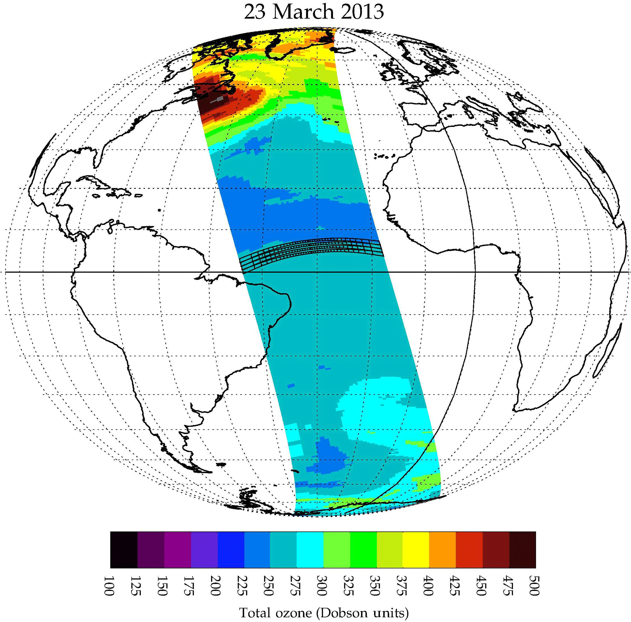
Figure 1Each orbit of NM data measures a swath of total column ozone: 35 individual ozone measurements (see example near the Equator) are made for each scan line.
The OMPS nadir profiler (NP) has a 16.6 µm cross-track slit and a 0.26 µm along-track slit width, producing a ground FOV cell size of 250 km by 250 km when exposed for a 38 s sample time. The OMPS NP instrument makes 80 measurements per orbit, resulting in full global coverage approximately every 6 days. The NP measures the complete spectrum from 250 to 310 nm with a 1.1 nm bandpass. Because the NP itself only makes measurements up to a maximum wavelength of 310 nm, the longer wavelengths that are needed in the retrievals at high latitudes must be taken by averaging the overlap cells from the NM instrument, the five central cross-track cells in five along-track scans.
The goal of the version 2 processing is to produce ozone data sufficiently accurate to be used to continue the Merged Ozone Data (MOD) time series. This time series is a unified multi-instrument ozone data set created by merging data from a series of SBUV and SBUV/2 instruments beginning with the original BUV instrument launched on Nimbus 4 in 1970 and extending to the SBUV/2 instrument on NOAA 19, which continues to operate. Data from these instruments were recently reprocessed as version 8.6 with a consistent calibration to create a coherent ozone time series (McPeters et al., 2013). The MOD data set created from this series is described in detail by Frith et al. (2014). Figure 2 shows the MOD fit to data from three recent SBUV/2 instruments, on NOAA 16, 18, and 19, for which good data are available during the OMPS observation period. Comparison with ozone from ground networks shows that total ozone in the MOD series is consistent to within about a percent for the recent data. Data from the OMPS NP and NM instruments will be used to extend this MOD data record.

Figure 2OMPS ozone will be compared with MOD (merged ozone data) ozone created by merging data from recent SBUV/2 instruments. Monthly average ozone for 60∘ S–60∘ N is plotted.
In the version 2 processing we use the latest version of the Level 1 data, the data set of calibrated radiance measurements from NM and NP that implements a refined calibration for both instruments (Seftor et al., 2014) and corrects for several instrument effects. Both the NM and NP L1b data now use an improved set of calibration coefficients that exhibit smoother wavelength-to-wavelength behavior and provide a wavelength registration that accounts for intra-orbital (for the NM) and intra-seasonal (for the NP) shifts that were identified in analysis of the data. A small bandpass error in the NP instrument near 295 nm was corrected, and errors in the pre-launch calibration measurements in the dichroic transition region (300–310 nm) for both instruments were identified and corrected. The daily dark current correction has been refined for each instrument.
Soft (in orbit) calibration techniques were used to refine the instrument calibration. The NM pre-launch calibration of the 331 nm channel, which is used to determine reflectivity, was not adjusted at nadir since the measured radiance over ice matched the expected radiance (determined from other instruments such as Earth Probe TOMS and OMI) to within 1 %. Cross-track adjustments to this channel to “flatten” the 331 nm reflectivity calculation over ice were then determined and applied. Similarly, the nadir radiance at 317 nm, which is the channel used to determine ozone, was not changed; the off-nadir radiances were then adjusted to take out any cross-track ozone dependence. The 317 and 331 nm NM nadir radiances are also used in the NP algorithm retrieval, with no adjustments applied. For the NM radiances at 312 nm, which are used in the NP algorithm but not in the NM algorithm, an adjustment was determined and applied to minimize the final retrieval residuals. Similarly, the NP 306 nm radiances were adjusted to minimize the final residuals. The calibrations were not explicitly adjusted to agree with the NOAA 19 SBUV/2 calibration, so NOAA 19 comparisons can be used for validation.
The algorithm used to retrieve total column ozone from the NM is very similar to the v8.5 algorithm used in the processing of data from Aura OMI instrument as described by Bhartia (2007) and Bhartia et al. (2004). The basic algorithm uses two wavelengths to derive total column ozone, one wavelength with weak ozone absorption (331 nm) to characterize the underlying surface and clouds, and the other at a wavelength with strong ozone absorption (317 nm). The ozone retrieval algorithms for both the NP and NM instruments now use the Brion–Daumont–Malicet ozone cross sections (Brion et al., 1993) to be consistent with other data sets in the MOD time series.
The NP retrieval algorithm uses 12 discrete wavelengths to retrieve ozone profiles employing Rodgers' optimal estimation technique (Bhartia et al., 2013). It is very similar to the v8.6 algorithm used to reprocess the SBUV and SBUV/2 data sets (McPeters et al., 2013) used in the MOD time series. While the vertical resolution of an OMPS NP ozone retrieval is somewhat coarse in comparison with the LP sensor, about 8 km resolution in the stratosphere, NP provides valuable data for the continuation of the historical SBUV/2 ozone data record, and for validation of the OMPS LP retrievals.
The accuracy and stability of the OMPS ozone data record has been evaluated through comparisons with ground-based observations and comparisons with other satellite data sets. The worldwide network of Dobson and Brewer stations has been used for years for ground-based validation of total column ozone. For satellite validation of total ozone, comparisons with the MOD data set are used as a primary standard for this evaluation. Validation of profile ozone (in Sect. 5) will use data from balloon sondes, data from the currently operating SBUV/2 instrument on NOAA 19, and data from the microwave limb sounder (MLS) on the Aura spacecraft.
Figure 3 compares average ozone from 52 ground-based Brewer and Dobson stations in the Northern Hemisphere with coincident observations of ozone measured by the NM instrument over the individual stations (Labow et al., 2013). Comparison with ozone from the NOAA 19 SBUV/2 is also shown (in blue) since these data are the basis of much of the NM and NP validation. Northern Hemisphere comparisons are shown because the network density is much better in the Northern Hemisphere than in the Southern Hemisphere, and comparisons in a single hemisphere will illuminate any seasonally dependent errors. Such comparisons have been shown to be capable of detecting instrument changes over the long term of a few tenths of a percent (McPeters et al., 2008). The comparison covers the period from April 2012 through the end of 2016. Figure 3 shows that the agreement of NM total ozone is mostly within half a percent. The linear fit in Fig. 3 shows that OMPS NM has very little drift in ozone relative to the ground observations (0.8 % per decade) and an average bias of less than 0.2 %.
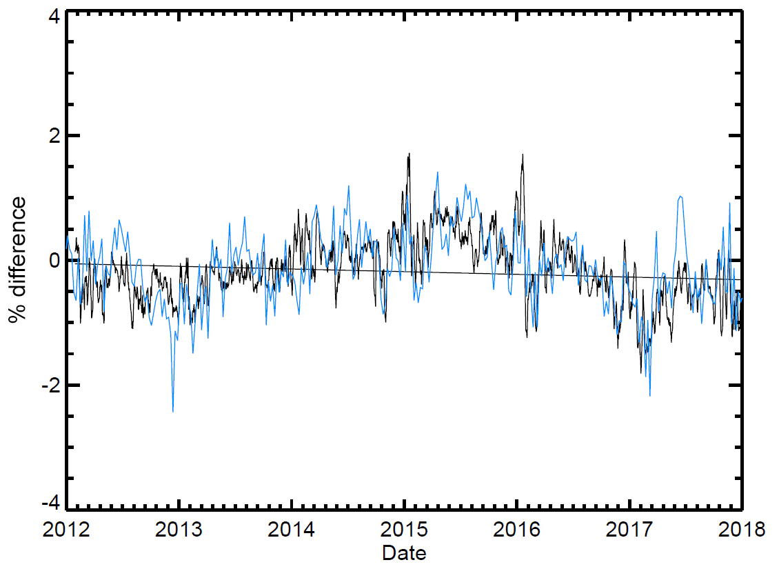
Figure 3A comparison of OMPS NM ozone (in black) and NOAA 19 SBUV (in blue) with average ozone from an ensemble of 52 Northern Hemisphere Dobson and Brewer stations. A linear fit to the NM data is also shown. Weekly mean percent difference of satellite ozone minus ground-based ozone is plotted.
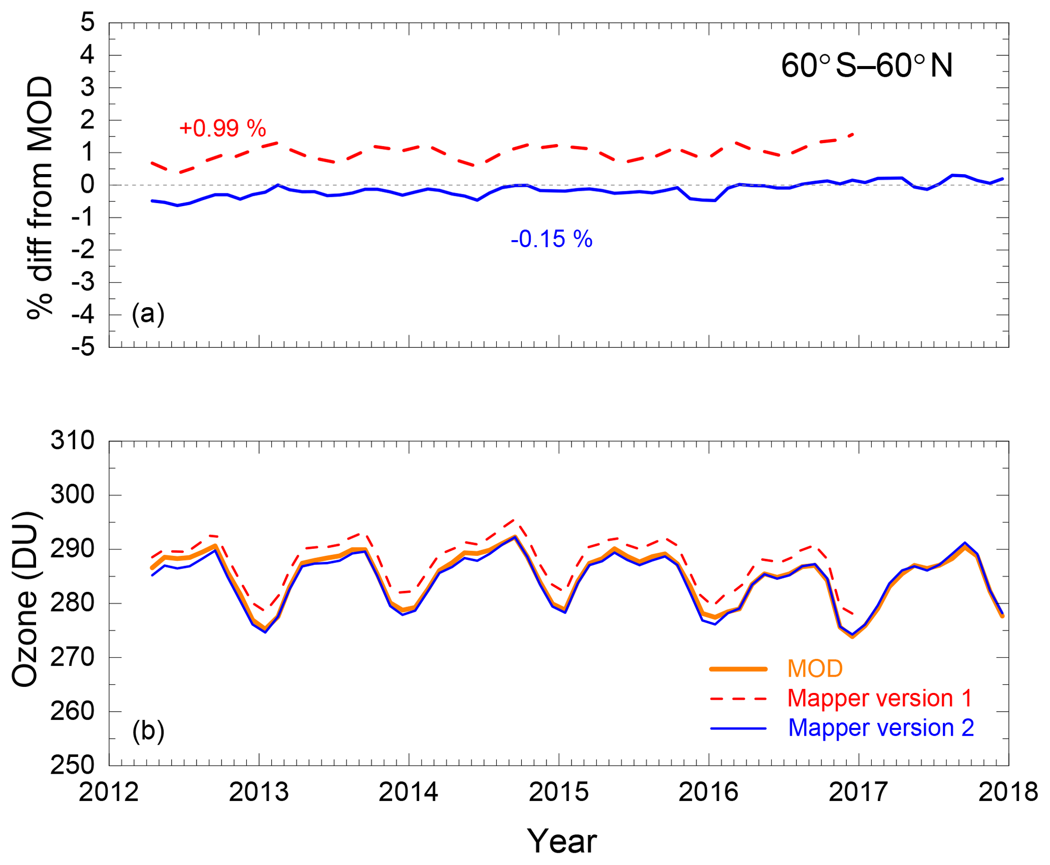
Figure 4For average ozone in the 60∘ S–60∘ N latitude zone (b), the average bias of NM ozone relative to MOD (a) was reduced from 0.99 % in version 1 to −0.20 % in the version 2 processing.
The comparison of ozone from the NM instrument with ozone from the MOD (merged ozone data set) time series shown in Fig. 4 illustrates the improved accuracy of the version 2 processing. The monthly zonal average ozone, area weighted for the latitude zone from 60∘ S to 60∘ N, is plotted. Because ozone is derived from measurements of backscattered sunlight, data are not always available in winter months at latitudes above 60∘. MOD ozone for this time period is based on combining ozone from SBUV/2 instruments on three satellites: NOAA 16, 18, and 19. For the period from March 2014 to 2017 only the instrument on NOAA 19 was operational. Figure 4b shows the NM monthly average ozone for the old version 1 processing (dashed red curve) and the new version 2 processing (solid blue curve) along with MOD average ozone (orange curve). Figure 4a shows the percent difference of version 1 and version 2 ozone from MOD ozone. While in version 1 NM ozone was on average 1 % higher relative to MOD, in the version 2 processing it is 0.2 % lower. There is a small relative trend between NM and MOD of 0.8 % per decade. This relative trend could be due to either NM or to an aging NOAA 19 SBUV/2 instrument in a drifting orbit. Further comparisons will be needed to distinguish between the two possibilities.
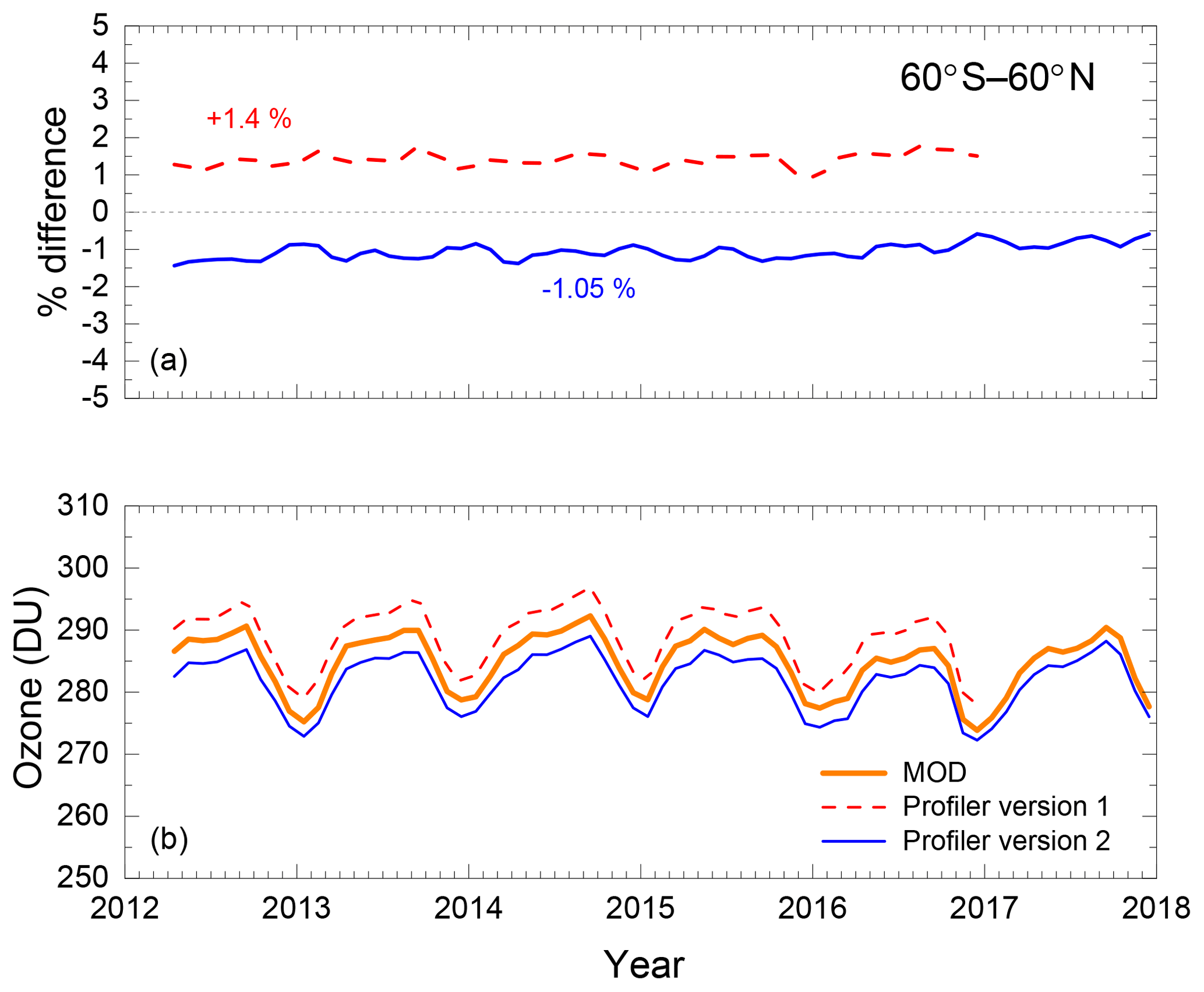
Figure 5A similar plot for the OMPS nadir profiler shows that the large bias in the released version 1 data is reduced in the version 2 processing.
Figure 5 is the same plot but for total column ozone measured by the NP instrument. NP total column ozone is derived by integrating the retrieved ozone profiles. In principle, this should be more accurate over a broad range of solar zenith angles than ozone derived from the limited wavelength range of the NM instrument. Here the average relative bias of about +1.4 % in version 1 is reduced to −1.05 % in version 2. This bias disagreement between NM and NP means that there is a small inconsistency between the two instruments that has not been resolved. This issue of the relative calibration inconsistency is being studied. There is a relative drift of NP ozone relative to MOD that is similar to that for the NM instrument, of 0.5 % per decade. To the extent that the NP and NM instruments have independent calibrations, this suggests that the small relative drift is due to the NOAA 19 SBUV/2 instrument calibration and the effect of the drifting orbit.
Figure 6 shows the latitude dependence relative to MOD of the version 2 ozone from the mapper and from the profiler. Figure 6b plots ozone averaged for five Marches from 2013 through 2016, while Fig. 6a shows the percent difference from MOD for the same months. The latitude dependence of ozone varies by season so it is useful to examine individual months, and latitude coverage is maximum near an equinox. The NM instrument has very little latitude dependence except at the highest southern latitudes where ozone is low. The NP instrument has the bias as noted in Fig. 5 and likewise has little latitude dependence at low to midlatitudes. The higher ozone (by 2 % to 3 %) for retrievals at latitudes greater than 50∘ may be a solar zenith angle dependent manifestation of what is possibly an NP calibration error.
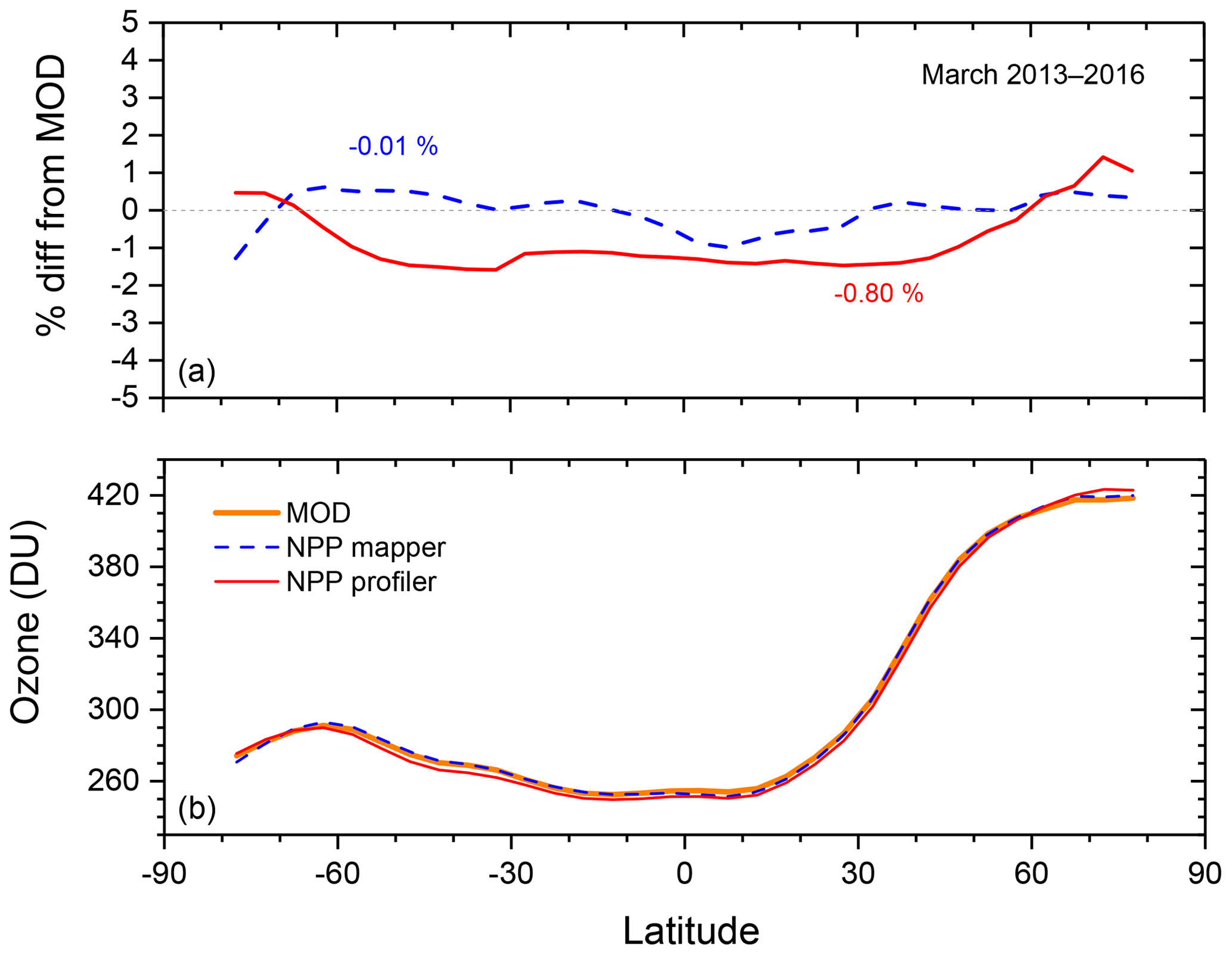
Figure 6In version 2 the 4-year average of March ozone latitude dependence (2013–2016) is shown in (b) for the mapper (dashed blue curve) and for the profiler (solid red curve). Percent differences from MOD are shown in (a).
The long-term behavior of ozone as a function of altitude is in some ways more interesting than the behavior of total column ozone because it can be used to confirm the accuracy of various model predictions. However, the accuracy of these measurements is more difficult to validate (Hassler et al., 2014). Data from the ozone sonde network can be used to validate the profile in the troposphere and lower stratosphere, while satellite data can be used to validate the middle to upper stratospheric results. There are ground-based measurements of the ozone vertical distribution by lidar and by microwave sounders, but such measurements are very sparse. There are Umkehr measurements by Dobson and Brewer instruments, but vertical resolution is coarse and uncertainty is high, especially when aerosols are present.

Figure 7An average of ozone sonde data from Hilo, Hawaii, is compared with OMPS NP version 2 ozone profiles for coincident days, with percent difference plotted in (b). The NP profile integrates to 274.1 DU, while the sonde profile integrates to 272.5 DU when a climatological stratospheric amount is added.
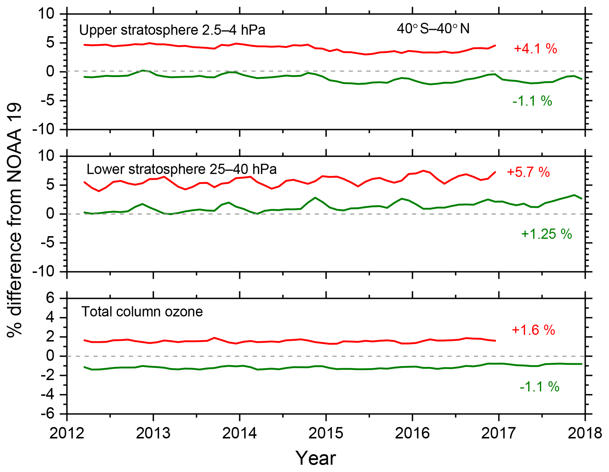
Figure 8The NP ozone anomaly, the difference from NOAA 19 ozone, for midlatitudes and low latitudes is shown as a function of time for total column ozone, the lower stratosphere, and the upper stratosphere. Ozone from the version 1 processing (in red) and the version 2 processing (in green) is shown.
Looking at ground-based comparisons of ozone in the lower stratosphere first, Fig. 7 compares NP ozone profiles with ozone measured by ECC ozone sondes from one station, Hilo, Hawaii (20∘ N, 155∘ W), a subtropical station with a good time series of sonde launches. The sonde data are from the SHADOZ network, under which the sonde data were reprocessed to apply the most recent corrections (Witte et al., 2016). For this figure, all 33 of the sondes launched in 2016 were averaged. The coincident profiles measured by NP were usually within 1∘ of latitude and within 15∘ of longitude. The comparison shows that in the lower stratosphere NP agrees with sonde data to within ±5 %. Only altitudes between 10 and 50 hPa (approximately 20 to 32 km) are shown because the SBUV nadir ozone retrieval algorithm produces little profile information on the distribution of ozone below 20 km. But it should be noted that the column amount of ozone in the troposphere is retrieved accurately (Bhartia et al., 2013), as evidenced by the fact that total column ozone from an SBUV retrieval is accurate to 1 % or better (McPeters et al., 2013). This accuracy is critical to the derivation of tropospheric ozone discussed in Sect. 6.

Figure 9OMPS NP version 2 June zonal average ozone profiles (2012–2016) compared with NOAA 19 SBUV/2 profiles, MLS profiles, and profiles from the OMPS LP. OMPS NP version 2 percent differences from N19, MLS, and LP are plotted on the right.
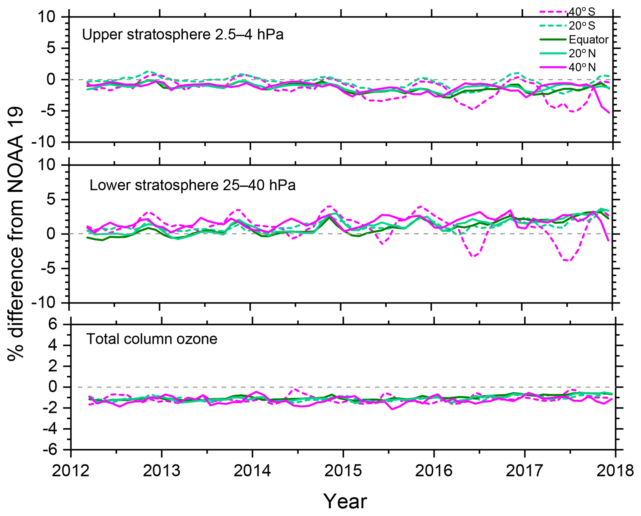
Figure 10The time dependence of the version 2 ozone anomaly relative to NOAA 19 shown for low to midlatitudes.
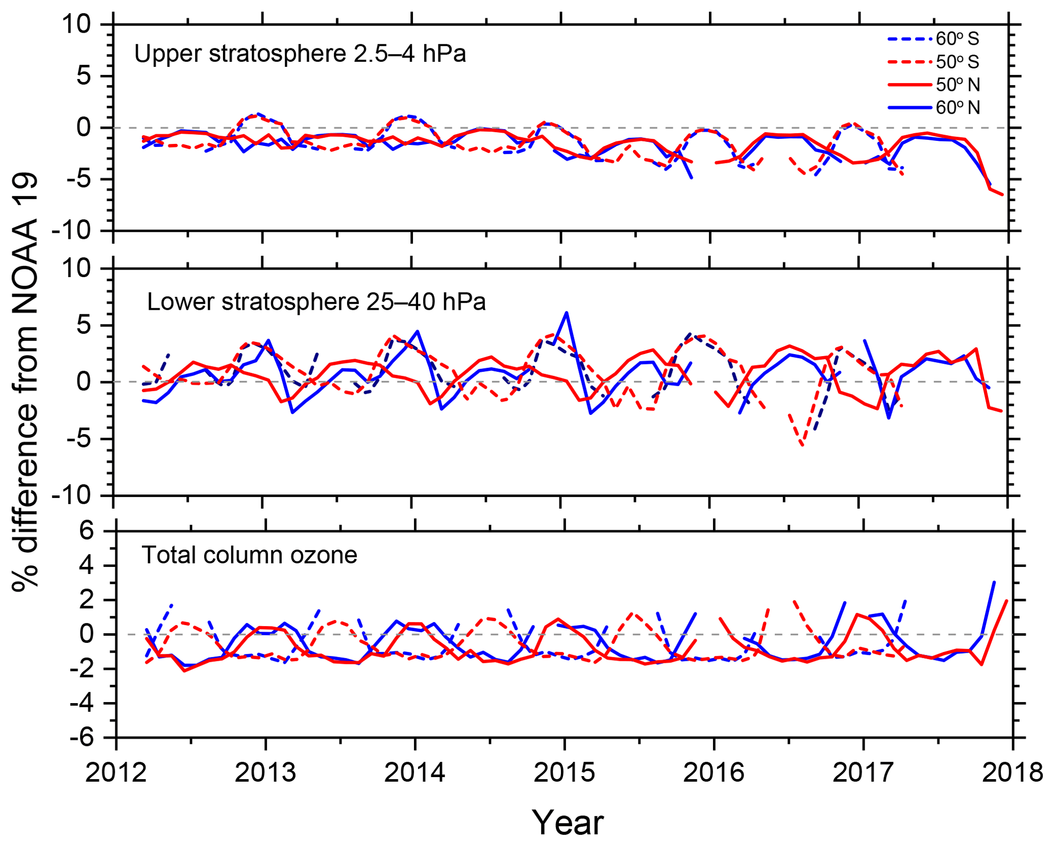
Figure 11The time dependence of the version 2.0 ozone anomaly relative to NOAA 19 shown for high latitudes.
For the middle to upper stratosphere, monthly zonal mean comparison with other satellite observations of the ozone vertical distribution is the best approach for evaluating the accuracy of the version 2 NP results. Figure 8 shows the time-dependent difference of NP from the NOAA 19 SBUV/2 retrievals averaged over low to middle latitudes (40∘ S to 40∘ N), for the upper stratosphere (2.5–4 hPa), lower stratosphere (25–40 hPa), and total column ozone. Comparing with N19 only rather than MOD gives a bit more uniformity for the time-dependent profile comparison. In both the upper stratosphere and lower stratosphere the version 2 ozone agrees with the N19 ozone to within about 1 %, where in the NP version 1 retrievals, ozone was higher by 4 % and 6 % respectively. There is no evidence of a significant time-dependent difference in total ozone, but in the middle stratosphere there appears to be a small increase in ozone of about 2 % over 6 years. There is the bias in total column ozone as noted earlier of a bit over 1 %. While the use of NM wavelengths in the NP retrieval may contribute to the bias, the bigger problem appears to be a wavelength-dependent calibration error in the NP itself. This possibility is being studied.
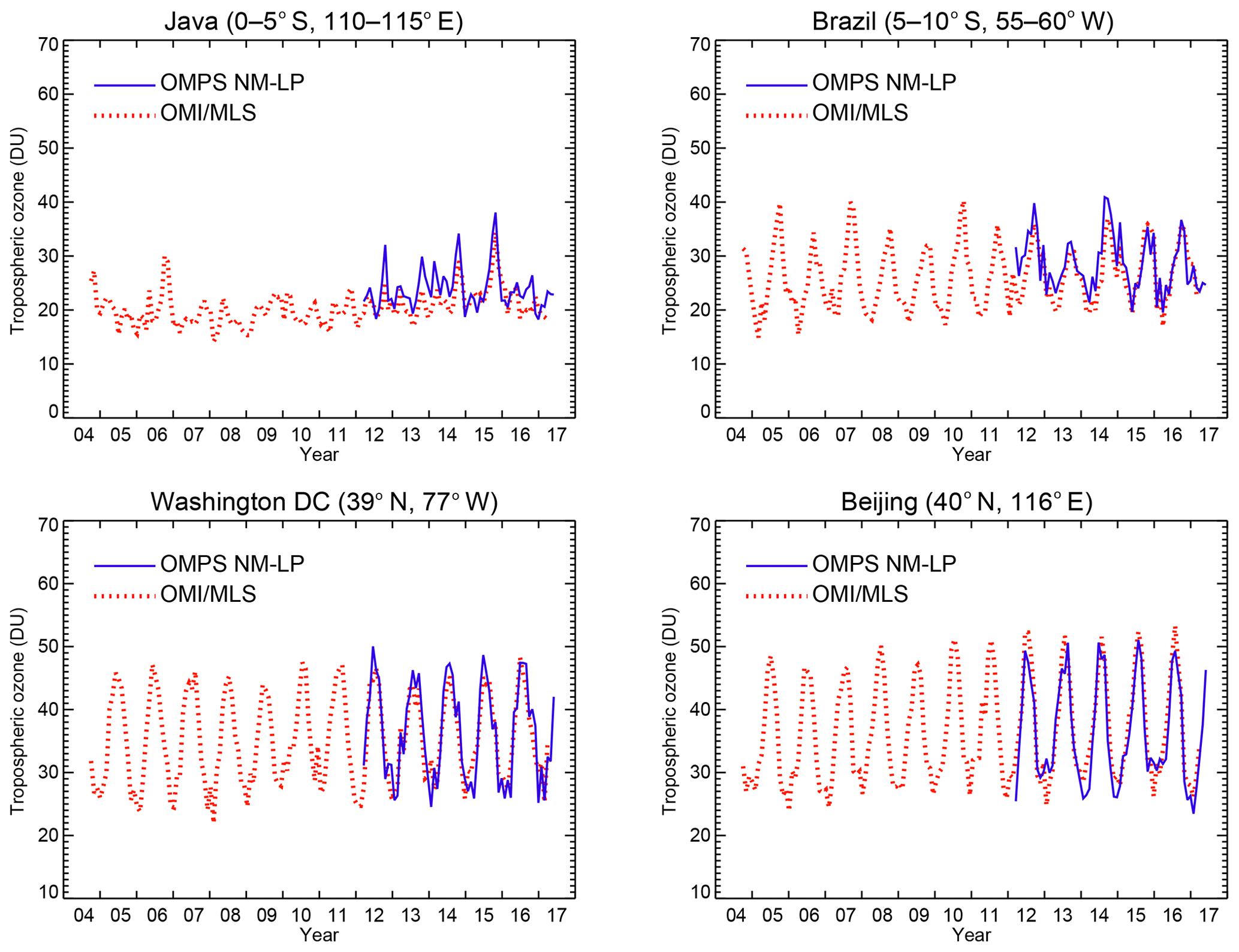
Figure 12The time series of tropospheric ozone shown for four locations. Tropospheric ozone derived by subtracting OMPS LP stratospheric ozone from NM total column ozone is shown in the blue solid curve, while tropospheric ozone derived by subtracting MLS stratospheric ozone from OMI total column ozone is shown in the dashed red curve.
Ozone agreement as a function of altitude is shown in Fig. 9 where ozone in low to middle latitudes is averaged for five Junes from 2012 through 2016. Selecting a single month for this comparison allows us to see any seasonal effect that might be suppressed in the annual average. As will be shown later, there are seasonal variations in NP ozone at high latitudes. The stratospheric ozone mixing ratio is plotted for OMPS NP version 2, for NOAA 19 SBUV/2, for the Aura microwave limb sounder (MLS) (Froidevaux et al., 2008), and for the OMPS limb profiler (LP). The right panel shows the agreement of the OMPS NP version 2 ozone profile with each of the three other profile measurements by plotting the percent difference from each. Agreement is almost always within ±5 %, which experience has shown to be fairly good agreement for profile comparisons. While agreement in the upper stratosphere and lower stratosphere shown in Fig. 8 was good, Fig. 9 shows that there is a significant underestimate of ozone relative to NOAA 19, MLS and LP in the 6 to 10 hPa region. This is likely the source of much of the disagreement in total column ozone. It has been noted in other comparisons (Hassler et al., 2014) that NOAA 19 ozone is a bit high in the upper stratosphere relative to MLS profiles, and a similar result is seen here for the NP retrievals.
The NP version 2 ozone has a somewhat different behavior at low to midlatitudes than at high latitudes. The ozone anomaly, the percent difference of NP ozone from the NOAA 19 SBUV ozone, is shown for low to midlatitudes (<45∘) in Fig. 10, and for higher latitudes (>45∘) in Fig. 11. For each figure the anomaly is shown for total column ozone (lower panel), for lower stratospheric ozone (layer from 25 to 40 hPa) in the middle panel, and for upper stratospheric ozone (layer from 2.5 to 4 hPa) in the upper panel. Figure 10 shows that version 2 ozone at latitudes below 45∘ agrees well with N19 ozone, while Fig. 11 shows that at latitudes at 50∘ and above ozone has a significant seasonal dependence that differs from that of N19 with about 2 % to 4 % amplitude. This difference is likely another manifestation of a possible NP calibration error. While this error is small, we are working to resolve it in order to produce a better NP ozone product.
Ziemke et al. (2011, 2014, and references therein) have shown that tropospheric ozone can be derived by subtracting stratospheric ozone from total column ozone. This technique has most recently been applied by subtracting stratospheric ozone measured by the Aura MLS instrument from total column ozone measured by the Aura OMI instrument. The OMI/MLS tropospheric ozone time series currently spans over 12 years and has been a central data product for each of the BAMS State of the Climate Reports since 2013 and will be used in the upcoming international Tropospheric Ozone Assessment Report.
The OMPS ozone measurements can also be used to calculate tropospheric ozone and continue the current OMI/MLS time series of measurements should either of the Aura instruments fail. Because the OMPS instrument suite includes both a total ozone mapper (NM) and a limb profiler (LP), a similar technique can be applied as with OMI/MLS. Figure 12 shows the tropospheric ozone time series for two locations in the tropics, Java and Brazil, and two locations at northern midlatitudes, Beijing and Washington DC. In each case the red dashed curve shows tropospheric ozone derived by subtracting MLS stratospheric ozone from OMI total column ozone. For comparison, the blue solid curve shows the same tropospheric ozone derived by subtracting stratospheric ozone from the OMPS LP from total column ozone from the NM. While there are some small differences the overall agreement is quite good. Data on tropospheric ozone from the NP plus LP combination can be used to continue the tropospheric ozone time series.
The OMPS nadir mapper (NM) has proven to be a very stable instrument. Comparison with a network of 52 Northern Hemisphere ground-based Dobson and Brewer instruments shows very good agreement over the four years of operation, agreeing within ±0.5 % with near-zero trend. Total column ozone from the OMPS nadir mapper agrees with MOD ozone and with NOAA 19 SBUV/2 ozone with a bias of −0.2 % and a small time-dependent drift of 0.8 % per decade. It is possible that this time dependence could be due to the aging NOAA 19 instrument and its drifting orbit.
The nadir profiler (NP) has likewise been very stable. NP total column ozone has a time dependence of only 0.5 % per decade relative to MOD or NOAA 19. The bias of −1.1 % (60∘ S–60∘ N) is small but inconsistent with ozone from NM. This bias seems to be generated in part by the negative bias in the 6–10 hPa region. The calibration of the NP instrument near 300 nm is being examined to understand this inconsistency. NP ozone in the upper stratosphere (2.5–4 hPa) and in the lower stratosphere (25–40 hPa) agrees well with ozone from NOAA 19 profiler, with an average difference of −1.1 % and +1.1 % respectively at latitudes below 50∘. The retrievals for higher latitudes exhibit a strong seasonal variation of about ±2 %, both in layer ozone and in total column ozone.
Ozone data from these instruments can now be considered “trend quality” – usable to extend the data record from previous instruments to create an accurate time series. Data from NP at latitudes above 50∘ appear to be stable but must be used with a bit of caution because of its residual seasonal variation and because the bias, while small, can be different than at lower latitudes.
NPP OMPS version 2 data are now available online from the Goddard DISC: https://disc.gsfc.nasa.gov (last access: 13 February 2019). Data for the NM mapper and the NP profiler are currently being converted to HDF5 format for inclusion in the DISC data archive. The calibrated L1 data are also available from the Goddard DISC. The OMPS NM ozone data are also available in ASCII form from our site: https://acd-ext.gsfc.nasa.gov/anonftp/toms/ (last access: 13 February 2019) in the subdirectory omps_tc. Data from the NOAA 19 SBUV/2 can also be found here under subdirectory sbuv. The v8.6 MOD data used as our standard for comparison are available from https://acdb-ext.gsfc.nasa.gov (last access: 13 February 2019): click on “Data_services” and then on “Merged ozone data”.
The authors declare that they have no conflict of interest.
The OMPS nadir profiler and nadir mapper were built by Ball Brothers for
flight on the joint NASA–NOAA NPP satellite. We thank the many people who
have worked over the years to understand the behavior of the OMPS
instrument. The Ozone Processing Team has carefully maintained the
calibration of the nadir instruments through both hard and soft calibration
techniques.
Edited by: Diego Loyola
Reviewed by: two anonymous referees
Bhartia, P. K., Wellemeyer, C. G., Taylor, S., Nath, N., and Gopolan, A.: Solar backscatter ultraviolet (SBUV) version 8 profile algorithm, in: Proceedings of the Quadrennial Ozone Symposium, Kos, Greece, 1–8 June 2004, 295–296, 2004.
Bhartia, P. K.: Total ozone from backscattered ultraviolet measurements, in: Observing Systems 20 for Atmospheric Composition, L'Aquila, Italy, 20–24 September 2004, edited by: Visconti, G., Di Carlo, P., Brune, W., Schoeberl, W., and Wahner, A., Springer, 48–63, 2007.
Bhartia, P. K., McPeters, R. D., Flynn, L. E., Taylor, S., Kramarova, N. A., Frith, S., Fisher, B., and DeLand, M.: Solar Backscatter UV (SBUV) total ozone and profile algorithm, Atmos. Meas. Tech., 6, 2533–2548, https://doi.org/10.5194/amt-6-2533-2013, 2013.
Brion, J., Chakir, A., Daumont, D., Malicet, J., and Parisse, C.: High resolution laboratory absorption cross section of O3 temperature effect, Chem. Phys. Lett., 213, 610–612, 1993.
Flynn, L. E., Seftor, C. J., Larsen, J. C., and Xu, P.: The Ozone Mapping and Profiler Suite, in: Earth Science Satellite Remote Sensing, edited by: Qu, J. J., Gao, W., Kafatos, M., Murphy, R. E., and Salomonson, V. V., Springer, Berlin, 279–296, https://doi.org/10.1007/978-3-540-37293-6, 2006.
Frith, S. M., Kramarova, N. A., Stolarski, R. S., McPeters, R. D., Bhartia, P. K., and Labow, G. J.: Recent changes in total column ozone based on the SBUV Version 8.6 merged ozone data set, J. Geophys. Res., 119, 9735–9751, https://doi.org/10.1002/2014JD021889, 2014.
Froidevaux, L., Jiang, Y., Lambert, A., Livesey, N., Read, W., Waters, J., Browell, E., Hair, J., Avery, M., McGee, T., Twigg, L., Sumnicht, G., Jucks, K., Margitan, J., Sen, B., Stachnik, R., Toon, G., Bernath, P., Boone, C., Walker, K., Filipiak, M., Harwood, R., Fuller, R., Manney, G., Schwartz, M., Daffer, W., Drouin, B., Cofield, R., Cuddy, D., Jarnot, R., Knosp, B., Perun, V., Snyder, W., Stek, P., Thurstans, R., and Wagner, P.: Validation of Aura Microwave Limb Sounder stratospheric and mesospheric ozone measurements, J. Geophys. Res., 113, D15S20, https://doi.org/10.1029/2007JD008771, 2008.
Hassler, B., Petropavlovskikh, I., Staehelin, J., August, T., Bhartia, P. K., Clerbaux, C., Degenstein, D., Mazière, M. D., Dinelli, B. M., Dudhia, A., Dufour, G., Frith, S. M., Froidevaux, L., Godin-Beekmann, S., Granville, J., Harris, N. R. P., Hoppel, K., Hubert, D., Kasai, Y., Kurylo, M. J., Kyrölä, E., Lambert, J.-C., Levelt, P. F., McElroy, C. T., McPeters, R. D., Munro, R., Nakajima, H., Parrish, A., Raspollini, P., Remsberg, E. E., Rosenlof, K. H., Rozanov, A., Sano, T., Sasano, Y., Shiotani, M., Smit, H. G. J., Stiller, G., Tamminen, J., Tarasick, D. W., Urban, J., van der A, R. J., Veefkind, J. P., Vigouroux, C., von Clarmann, T., von Savigny, C., Walker, K. A., Weber, M., Wild, J., and Zawodny, J. M.: Past changes in the vertical distribution of ozone – Part 1: Measurement techniques, uncertainties and availability, Atmos. Meas. Tech., 7, 1395–1427, https://doi.org/10.5194/amt-7-1395-2014, 2014.
Labow, G., McPeters, R., Bhartia, P. K., and Kramarova, N.: A comparison of 40 years of SBUV measurements of column ozone with data from the Dobson/Brewer network, J. Geophys. Res., 118, 7370–7378, https://doi.org/10.1002/jgrd.50503, 2013.
McPeters, R. D., Kroon, M., Labow, G., Brinksma, E., Balis, D., Petropavlovskikh, I., Veefkind, J., Bhartia, P. K., and Levelt, P.: Validation of the Aura Ozone Monitoring Instrument total column ozone product, J. Geophys. Res., 113, D15S14, https://doi.org/10.1029/2007JD008802, 2008.
McPeters, R. D., Bhartia, P. K., Haffner, D., Labow, G., and Flynn, L.: The version 8.6 SBUV ozone data record: an overview, J. Geophys. Res., 118, 1–8, https://doi.org/10.1002/jgrd.50597, 2013.
Seftor, C. J., Jaross, G., Kowitt, M., Haken, M., Li, J., and Flynn, L., Postlaunch performance of the Suomi National Polar orbiting Partnership Ozone Mapping and Profiler Suite (OMPS) nadir sensors, J. Geophys. Res.-Atmos., 119, 4413–4428, https://doi.org/10.1002/2013JD020472, 2014.
Witte, J. C., Thompson, A., Smit, H., Fujiwara, M., Posny, F., Coetzee, G., Northam, E., Johnson, B., Sterling, C., Mohamad, M., Ogino, S., Jordan, A., and da Silva, F.: First reprocessing of Southern Hemisphere ADditional OZonesondes (SHADOZ) profile records (1998–2015): 1. Methodology and evaluation, J. Geophys. Res.-Atmos., 122, 6611–6636, https://doi.org/10.1002/2016JD026403, 2016.
Ziemke, J. R., Chandra, S., Labow, G. J., Bhartia, P. K., Froidevaux, L., and Witte, J. C.: A global climatology of tropospheric and stratospheric ozone derived from Aura OMI and MLS measurements, Atmos. Chem. Phys., 11, 9237–9251, https://doi.org/10.5194/acp-11-9237-2011, 2011.
Ziemke, J. R., Olsen, M., Witte, J., Douglass, A., Strahan, S., Wargan, K., Liu, X., Schoeberl, M., Yang, K., Kaplan, T., Pawson, S., Duncan, B., Newman, P., Bhartia, P. K., and Heney, M.: Assessment and applications of NASA ozone data products derived from Aura OMI/MLS satellite measurements in context of the GMI chemical transport model, J. Geophys. Res.-Atmos., 119, 5671–5699, https://doi.org/10.1002/2013JD020914, 2014.