the Creative Commons Attribution 4.0 License.
the Creative Commons Attribution 4.0 License.
 | 14 Feb 2019
The use of QBO, ENSO, and NAO perturbations in the evaluation of GOME-2 MetOp A total ozone measurements
Christos S. Zerefos
Dimitris S. Balis
Maria-Elissavet Koukouli
John Kapsomenakis
Diego G. Loyola
Pieter Valks
Melanie Coldewey-Egbers
Christophe Lerot
Stacey M. Frith
Amund S. Haslerud
Ivar S. A. Isaksen
Seppo Hassinen
In this work we present evidence that quasi-cyclical perturbations in total ozone (quasi-biennial oscillation – QBO, El Niño–Southern Oscillation – ENSO, and North Atlantic Oscillation – NAO) can be used as independent proxies in evaluating Global Ozone Monitoring Experiment (GOME) 2 aboard MetOp A (GOME-2A) satellite total ozone data, using ground-based (GB) measurements, other satellite data, and chemical transport model calculations. The analysis is performed in the frame of the validation strategy on longer time scales within the European Organisation for the Exploitation of Meteorological Satellites (EUMETSAT) Satellite Application Facility on Atmospheric Composition Monitoring (AC SAF) project, covering the period 2007–2016. Comparison of GOME-2A total ozone with ground observations shows mean differences of about % in the tropics (0–30∘), about % in the mid-latitudes (30–60∘), and about % and 0.0±4.3 % over the northern and southern high latitudes (60–80∘), respectively. In general, we find that GOME-2A total ozone data depict the QBO–ENSO–NAO natural fluctuations in concurrence with the co-located solar backscatter ultraviolet radiometer (SBUV), GOME-type Total Ozone Essential Climate Variable (GTO-ECV; composed of total ozone observations from GOME, SCIAMACHY – SCanning Imaging Absorption SpectroMeter for Atmospheric CHartographY, GOME-2A, and OMI – ozone monitoring instrument, combined into one homogeneous time series), and ground-based observations. Total ozone from GOME-2A is well correlated with the QBO (highest correlation in the tropics of +0.8) in agreement with SBUV, GTO-ECV, and GB data which also give the highest correlation in the tropics. The differences between deseazonalized GOME-2A and GB total ozone in the tropics are within ±1 %. These differences were tested further as to their correlations with the QBO. The differences had practically no QBO signal, providing an independent test of the stability of the long-term variability of the satellite data. Correlations between GOME-2A total ozone and the Southern Oscillation Index (SOI) were studied over the tropical Pacific Ocean after removing seasonal, QBO, and solar-cycle-related variability. Correlations between ozone and the SOI are on the order of +0.5, consistent with SBUV and GB observations. Differences between GOME-2A and GB measurements at the station of Samoa (American Samoa; 14.25∘ S, 170.6∘ W) are within ±1.9 %. We also studied the impact of the NAO on total ozone in the northern mid-latitudes in winter. We find very good agreement between GOME-2A and GB observations over Canada and Europe as to their NAO-related variability, with mean differences reaching the ±1 % levels. The agreement and small differences which were found between the independently produced total ozone datasets as to the influence of the QBO, ENSO, and NAO show the importance of these climatological proxies as additional tool for monitoring the long-term stability of satellite–ground-truth biases.
- Article
(14965 KB) - Full-text XML
-
Supplement
(1841 KB) - BibTeX
- EndNote


Ozone is an important gas of the Earth's atmosphere. In the stratosphere, ozone is considered good ozone, because it absorbs ultraviolet B radiation from the sun, thus protecting the biosphere from a large part of the sun's harmful radiation (e.g. Eleftheratos et al., 2012; Hegglin et al., 2015). In the lower atmosphere and near the surface, natural ozone has an equally important beneficial role, because it initiates the chemical removal of air pollutants from the atmosphere such as carbon monoxide, nitrogen oxides, and methane. Above natural levels, however, ozone is considered bad ozone because it can harm humans, plants, and animals. In addition, ozone is a greenhouse gas, warming the Earth's surface. In both the stratosphere and the troposphere, ozone absorbs infrared radiation emitted from Earth's surface, trapping heat in the atmosphere. As a result, increases or decreases in stratospheric or tropospheric ozone induce a climate forcing (Hegglin et al., 2015).
Ozone in the atmosphere can be measured by ground-based (GB) instruments, balloons, aircraft, and satellites and can be calculated by chemical transport model (CTM) simulations. Measurements by satellites from space provide ozone profiles and column amounts over nearly the entire globe on a daily basis (e.g. WMO, 2014). The three Global Ozone Monitoring Experiment 2 (GOME-2) instruments carried on MetOp platforms A, B, and C (GOME-2A, GOME-2B, and GOME-2C, respectively) serve this purpose. The first was launched on 19 October 2006, the second on 19 September 2012, and the last on 7 November 2018. The three GOME-2 instruments will provide unique long-term datasets of more than 15 years (2007–2024) related to atmospheric composition and surface ultraviolet radiation using consistent retrieval techniques (Hassinen et al., 2016). The GOME-2 offline data are set to make a significant contribution towards climate and atmospheric research while providing near real-time data for use in weather forecasting and air quality forecasting applications (Hassinen et al., 2016).
Validation of satellite ozone measurements is performed with ground-based measurements as well as other satellite instruments (Hassinen et al., 2016). Validation of GOME-2A total ozone for the period 2007–2011 was performed by Loyola et al. (2011) and Koukouli et al. (2012). It was found that GOME-2 total ozone data agree at the ±1 % level with GB measurements and other satellite datasets (Hassinen et al., 2016). The consistency between GOME-2A and GOME-2B total ozone columns, including a validation with GB measurements, was presented by Hao et al. (2014). An updated time series of the differences between GOME-2A and GOME-2B with GB observations can be found in Hassinen et al. (2016). The long-term stability of the two satellite instruments was also noted in that study. Both satellites are consistent over the Northern Hemisphere with negligible latitudinal dependence, while over the Southern Hemisphere there is a systematic difference of 1 % between the two satellite instruments (Hassinen et al., 2016).
Chiou et al. (2014) compared zonal mean total column ozone inferred from three independent multi-year data records, namely solar backscatter ultraviolet radiometer (SBUV; v8.6) total ozone (McPeters et al., 2013), GOME-type Total Ozone Essential Climate Variable (GTO-ECV; Coldewey-Egbers et al., 2015; Garane et al., 2018), and GB total ozone for the period 1996–2011. Their analyses were conducted for the latitudinal zones of 0–30∘ S, 0–30∘ N, 50–30∘ S, and 30–60∘ N. It was found that, on average, the differences in monthly zonal mean total ozone vary between −0.3 % and 0.8 % and are well within 1 %. In that study it was concluded that, despite the differences in the satellite sensors and retrievals methods, the SBUV v8.6 and GTO-ECV data records show very good agreement both in the monthly zonal mean total ozone and the monthly zonal mean anomalies between 60∘ S and 60∘ N. The GB zonal means showed larger scatter in the monthly mean data compared to satellite-based records, but the scatter was significantly reduced when seasonal zonal averages were analysed. The differences between SBUV and GB total ozone data presented in Chiou et al. (2014) are well in agreement with Labow et al. (2013), who systematically compared SBUV (v8.6) total ozone data with those measured by Brewer and Dobson instruments at various stations as a function of time, satellite solar zenith angle, and latitude. The comparisons showed good agreement (within ±1 %) over the past 40 years, with the very small bias approaching zero over the last decade. Comparisons with ozone sonde data showed good agreement in the integrated column up to 25 hPa, with differences not exceeding 5 % (Labow et al., 2013).
The observed small biases (at the percentage level) between satellite and GB observations of total ozone, as have been documented in the above studies, ensure the provision of accurate satellite ozone measurements. The high accuracy and stability of the satellite instruments is essential for monitoring the expected recovery of the ozone layer resulting from measures adopted by the 1987 Montreal Protocol and its amendments (e.g. Zerefos et al., 2009; Loyola et al., 2011; Solomon et al., 2016; de Laat et al., 2017; Kuttippurath and Nair, 2017; Pazmiño et al., 2018; Stone et al., 2018; Strahan and Douglass, 2018). It is known that total ozone varies strongly with latitude and longitude as a result of chemical and transport processes in the atmosphere. Total ozone also varies with season. Seasonal variations are larger over mid-latitudes and high latitudes and are smaller in the tropics (e.g. WMO, 2014). On longer time scales total ozone variability is related to large-scale natural oscillations such as the quasi-biennial oscillation (QBO; e.g. Zerefos et al., 1983; Baldwin et al., 2001), the El Niño–Southern Oscillation (ENSO; e.g. Zerefos et al., 1992; Oman et al., 2013; Coldewey-Egbers et al., 2014), the North Atlantic Oscillation (NAO; e.g. Ossó et al., 2011; Chehade et al., 2014), and the 11-year solar cycle (e.g. Zerefos et al., 2001; Tourpali et al., 2007; Brönniman et al., 2013). Moreover, volcanic eruptions may also alter the thickness of the ozone layer (Zerefos et al., 1994; Frossard et al., 2013; Rieder et al., 2013; WMO, 2014). These natural perturbations affect the background atmosphere and consequently the distribution of the ozone layer. In this context, the study of the effect of known natural fluctuations in total ozone could serve as additional tool for evaluating the long-term variability of satellite total ozone data records.
The objective of the present work is to examine the ability of the GOME-2A total ozone data to capture the variability related to dynamical proxies of global and regional importance, such as the QBO, ENSO, and NAO, in comparison to GB measurements, other satellite data, and model calculations. The variability of total ozone from GOME-2A is compared with the variability of total ozone from the other examined datasets during these naturally occurring fluctuations in order to evaluate the ability of GOME-2A to depict natural perturbations. The analysis is performed in the frame of the validation strategy of GOME-2A data on longer time scales within the European Organisation for the Exploitation of Meteorological Satellites (EUMETSAT) Satellite Application Facility on Atmospheric Composition Monitoring (AC SAF) project. The evaluation of GOME-2A data performed here includes the study of monthly means of total ozone, the annual cycle of total ozone, the amplitude of the annual cycle (i.e. (maximum value – minimum value)/2), the relation with the QBO (correlation with zonal wind at the Equator at 30 hPa), the relation with ENSO (correlation with the Southern Oscillation Index – SOI), and the relation with the NAO (correlation with the NAO index in winter – DJF mean).
The annual cycle describes regular oscillations in total ozone that occur from month to month within a year. In general, month-to-month variations of total ozone are larger in the mid-latitudes and high latitudes than in the tropics. The QBO dominates the variability of the equatorial stratosphere (∼16–50 km) and is easily seen as downward-propagating easterly and westerly wind regimes, with a variable period averaging approximately 28 months. Circulation changes induced by the QBO affect temperature and chemistry (Baldwin et al., 2001). The ENSO and NAO are naturally occurring patterns or modes of atmospheric and oceanic variability which orchestrate large variations in climate over large regions with profound impacts on ecosystems (Hurrell and Deser, 2009). We present the level of agreement between satellite-derived GOME-2A and GB total ozone in depicting natural oscillations like the QBO, ENSO, and NAO, highlighting the importance of these climatological proxies to be used as additional tools for monitoring the long-term stability of satellite–ground-truth biases.
The analysis uses GOME-2 satellite total ozone columns for the period 2007–2016. This data forms part of the operational EUMETSAT AC SAF GOME-2 MetOp A GDP4.8 data product provided by the German Aerospace Center (DLR). The GOME-2 total ozone data have been averaged on a monthly latitude longitude grid. The overview of the GOME-2A satellite instrument and of the GOME-2 atmospheric data provided by AC SAF can be found in Hassinen et al. (2016).
To examine the natural variability of ozone on longer time scales, we have additionally analysed the Global Ozone Monitoring Experiment (GOME) aboard the second European Remote Sensing satellite (ERS-2), SCanning Imaging Absorption SpectroMeter for Atmospheric CHartographY (SCIAMACHY) on Envisat, GOME-2A, and ozone monitoring instrument (OMI) on Aura merged prototype level-3 harmonized data record (GTO-ECV, ) data for the period 1995–2016 (Coldewey-Egbers et al., 2015; Garane et al., 2018). This GTO-ECV ozone data product was generated and provided by DLR as part of the European Space Agency Ozone Climate Change Initiative (ESA O3 CCI). The ESA O3 CCI merged level-3 record, which is based on GOME–SCIAMACHY–GOME-2A–OMI level-2 data, was obtained using the GODFIT v3.0 retrieval algorithm. More on ESA O3 CCI datasets can be found in the studies by Van Roozendael et al. (2012), Lerot et al. (2014), Koukouli et al. (2015), and Garane et al. (2018).
Both datasets are compared with a combined Total Ozone Mapping Spectrometer (TOMS), OMI, and Ozone Mapping Profiler Suite (OMPS) satellite total ozone dataset constructed using data from the TOMS on Nimbus 7 (1979–1993); TOMS on Meteor 3 (1991–1994); TOMS on Earth Probe (1996–2005); the OMI aboard the NASA Earth Observing System (EOS) Aura satellite (2005–present); and data from the next-generation OMPS nadir profiler instrument, launched in October 2011 on the Suomi National Polar-orbiting Partnership (NPP) satellite (McPeters et al., 2015). The total ozone data are available at (TOMS) or (OMI–OMPS) resolution from https://acd-ext.gsfc.nasa.gov/anonftp/toms/ (last access: 15 June 2018). From these data we constructed monthly mean total ozone data on a grid. To account for known biases between the instruments (e.g. Labow et al., 2013) we use the SBUV v8.6 merged ozone dataset (MOD) monthly zonal mean total ozone (https://acd-ext.gsfc.nasa.gov/Data_services/merged/index.html, also see next paragraph; last access: 15 June 2018) as a reference. We adjust each instrument such that the zonal mean in each 5∘ band averaged over the instrument lifetime matches the corresponding SBUV MOD zonal mean average. Thus the inherent longitudinal variability is retained from the TOMS–OMI–OMPS measurements, but any latitude-dependent bias between the instruments is removed. With the exception of the Meteor 3 TOMS in the Northern Hemisphere, all offsets were within 2 % at low and mid-latitudes. Such a dataset should not be used for long-term trends but is sufficient for analysing periodic variability such as that for the QBO, ENSO, and NAO. We used data for the period 1995–2016. We note here that another long-term dataset which has been analysed for the QBO, ENSO, NAO and other perturbations comes from the multi-sensor reanalysis (MSR; Knibbe et el., 2014) but is not examined here.
In addition, we compare this with satellite SBUV station overpass data from 1995 to 2016. The satellite data are based on measurements from three SBUV-type instruments from April 1970 to the present (continuous data coverage from November 1978). Even though the time series includes different versions of the SBUV instrument, the basic measurement technique remains the same over the advancement of the instrument from the backscatter ultraviolet radiometer (BUV) to Solar Backscatter Ultraviolet Radiometer 2 (SBUV-2; Bhartia et al., 2013). Satellite overpass data over various ground-based stations are provided per day from https://acd-ext.gsfc.nasa.gov/anonftp/toms/sbuv/MERGED/ (last access: 15 June 2018). These overpass data are analogous to the SBUV MOD monthly zonal mean data previously mentioned. Both are constructed by first filtering measurements of lesser quality and then averaging data from individual satellites when more than one instrument is operating. Monthly averages have been calculated by averaging the daily merged ozone overpass data for stations listed in Supplement Table S1. Details about the data are provided by McPeters et al. (2013) and Frith et al. (2014).
We also compare this with GB observations of total ozone from a number of stations contributing to the World Ozone and Ultraviolet Radiation Data Centre (WOUDC). The WOUDC data centre is one of six world data centres which are part of the Global Atmosphere Watch programme of the World Meteorological Organization (WMO). The WOUDC data centre is operated by the Meteorological Service of Canada, a branch of Environment Canada. In total, we analysed total ozone daily summaries from 193 ground-based stations operating Brewer, Dobson, filter, Système D'Analyse par Observations Zénithales (SAOZ), or Microtops instruments. The GB total ozone measurements are available from the website https://woudc.org/archive/Summaries/TotalOzone/Daily_Summary/ (last access: 15 June 2018). The various stations used in this study are listed in Table S1.
We have also analysed simulations of total ozone from the global 3-D CTM, the Oslo CTM3 (Søvde et al., 2012). The Oslo CTM3 has traditionally been driven by 3-hourly meteorological forecast data from the European Centre for Medium-Range Weather Forecasts (ECMWF) Integrated Forecast System (IFS) model, whereas in this study we apply the OpenIFS model (https://software.ecmwf.int/wiki/display/OIFS/; last access: 15 June 2018), cycle 38r1, which is an improvement from Søvde et al. (2012). Details on the model are given in Søvde et al. (2012). The Oslo CTM3 comprises both detailed tropospheric and stratospheric chemistry. Photochemistry is calculated using Fast-JX version 6.7c (Prather, 2015) and chemical kinetics from the Jet Propulsion Laboratory (JPL) 2011 (Sander et al., 2011). Total ozone columns compare well with measurements and other model studies (Søvde et al., 2012 and references therein). The horizontal resolution of the model is . We used the global monthly mean total ozone columns for the period 1995–2016.
To examine the QBO component of total ozone we made use of the monthly mean zonal winds in Singapore at 30 hPa. The zonal wind data at 30 hPa were provided by the Freie Universität Berlin (FU-Berlin) at https://www.geo.fu-berlin.de/met/ag/strat/produkte/qbo/qbo.dat (last access: 15 June 2018; Naujokat, 1986). The impact of ENSO in the tropics was investigated by using the SOI from the Bureau of Meteorology of the Australian Government (http://www.bom.gov.au/climate/current/soi2.shtml; last access: 15 June 2018). The correlation between total ozone and the NAO index was mainly computed for the winter mean (DJF) when the NAO amplitude is large (e.g. Hurrell and Deser, 2009), but it is also addressed in other seasons. Emphasis is placed on Canada, Europe, and the North Atlantic Ocean in winter. The NAO index (DJF) based on the principal component (PC) provided by the Climate Analysis Section of NCAR in Boulder, CO, USA (available at: https://climatedataguide.ucar.edu/climate-data/hurrell-north-atlantic-oscillation-nao-index-pc-based; last access: 15 June 2018), was used. Total ozone variability is also related to dynamical variability, for example, variability in tropopause height (e.g. Dameris et al., 1995; Hoinka et al., 1996; Steinbrecht et al., 1998). The impact of tropopause height variations on total ozone variability was examined by analysing the tropopause pressure from the independently produced NCEP/NCAR (National Centers for Environmental Prediction – National Center for Atmospheric Research) Reanalysis 1 dataset computed on a 2.5∘ grid. The NCEP/NCAR reanalysis data were provided from the website at https://www.esrl.noaa.gov/psd/data/gridded/data.ncep.reanalysis.tropopause.html (last access: 15 June 2018; Kalnay et al., 1996).
Table 1Mean differences and their standard deviations in percent between total ozone from GOME-2A, SBUV (v8.6) satellite overpass data, and ground-based observations over different latitude zones, as shown in Figs. 1 and 2.

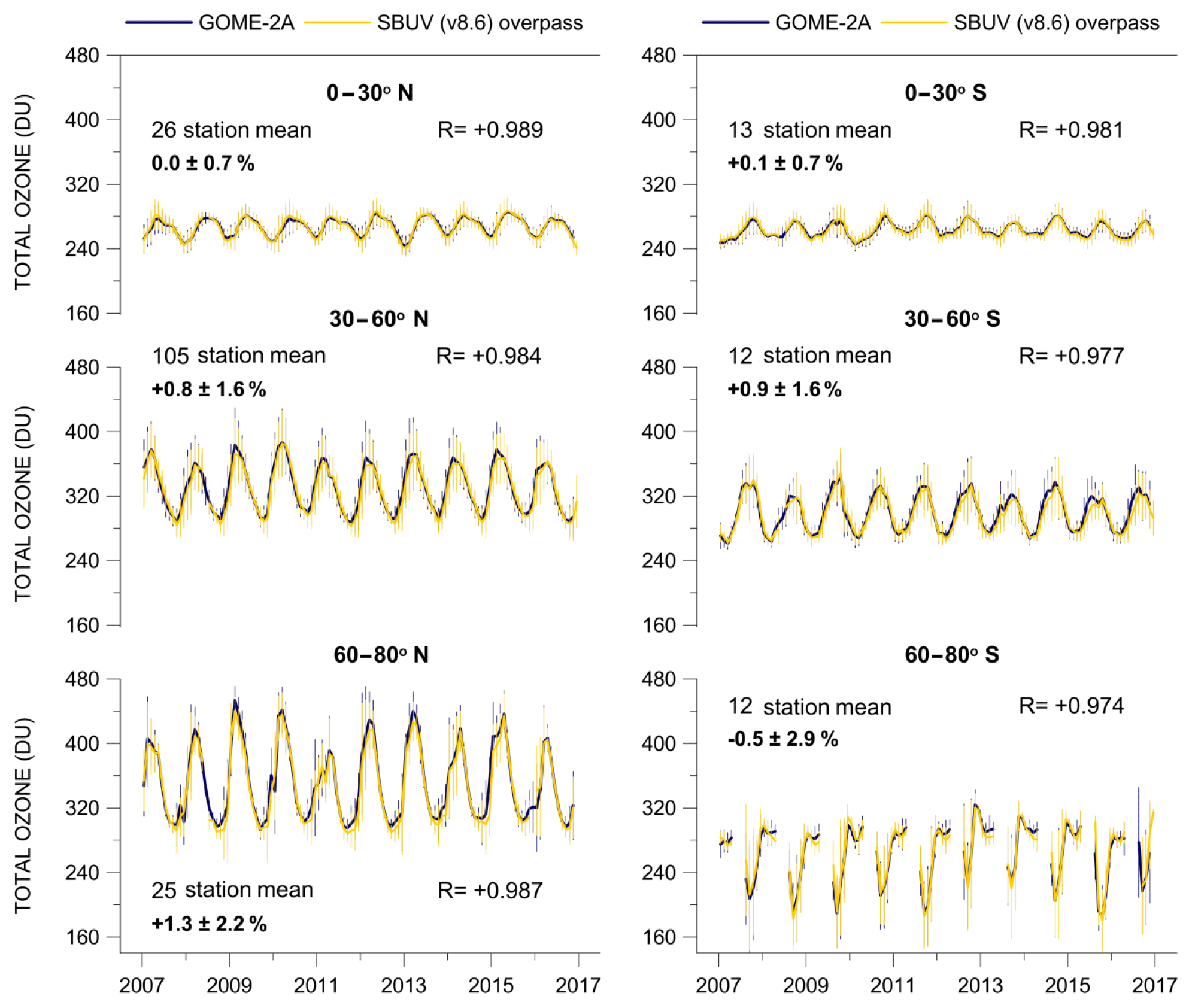
Figure 1Monthly mean total ozone from GOME-2A compared with monthly mean total ozone from SBUV (v8.6) satellite overpass data for the period 2007–2016 over the Northern and the Southern Hemisphere, based on station mean data. R is the correlation coefficient between the two lines. Error bars show the standard deviation of each monthly mean. Mean differences ±σ are given as (GOME-2A – SBUV)/SBUV (%).
3.1 Monthly zonal means and annual cycle
Figure 1 compares monthly mean total ozone from GOME-2A and SBUV (v8.6) satellite overpass data for stations shown in Table S1. The GOME-2A data were taken at a spatial resolution of around each of the ground-based monitoring stations listed in Table S1 and then averaged over the tropics, mid-latitudes, and high latitudes of both hemispheres in 30∘ latitudinal zones to provide the large-scale monthly zonal means for the GOME-2A data. Accordingly, SBUV satellite overpass data were averaged over each geographical zone to provide the large-scale zonal means for the SBUV observations. Mean differences and standard deviations between GOME-2A and SBUV total ozone were found to be % in the tropics (0–30∘), about % in the mid-latitudes (30–60∘), about % over the northern high latitudes (60–80∘ N), and about % over the southern high latitudes (60–80∘ S). The differences were estimated as (GOME-2A – SBUV)/SBUV (%) from January 2007 to December 2016. Small differences were also found between GOME-2A and GB measurements (Fig. 2 and Table 1), and here GB station data were averaged over each geographical zone to provide the large-scale zonal means for the GB measurements. Mean differences and standard deviations between GOME-2A and GB total ozone were found to be % in the tropics (0–30∘), % in the mid-latitudes (30–60∘), % over the northern high latitudes (60–80∘ N), and 0.0±4.3 % over the southern high latitudes (60–80∘ S). Recall that all estimates refer to the period between January 2007 and December 2016.
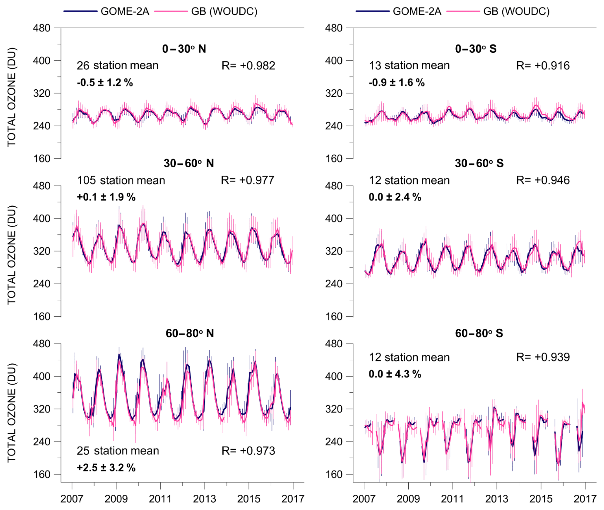
Figure 2Same as in Fig. 1, but for GOME-2A and GB observations. R is the correlation coefficient between the two lines. Error bars show the standard deviation of each monthly mean. Mean differences ±σ are given as (GOME-2A – GROUND)/GROUND (%).
In summary, the largest differences between GOME-2A, SBUV (v8.6), and GB measurements are found over the northern high latitudes (60–80∘ N), and the highest variability (standard deviation of the mean difference) is observed over the latitude belt (60–80∘ S). In addition, these differences (especially at the high latitudes) can be affected by the fact that the same days have not always been used for the construction of the monthly mean values for the different datasets. In the tropics and mid-latitudes the respective differences are within ±1 % or less, in line with Chiou et al. (2014). Validation results were also presented by Loyola et al. (2011), Koukouli et al. (2012), Coldewey-Egbers et al. (2015), and Koukouli et al. (2015), and updates of which are included in Hassinen et al. (2016). Our results based on data updated to 2017 largely confirm those studies, pointing to the good performance of GOME-2A when extending the period of record.
Table 2Statistics of the correlations shown in Figs. 1 and 2 between total ozone from (a) GOME-2A data and SBUV (v8.6) overpass data and (b) GOME-2A data and ground-based measurements.
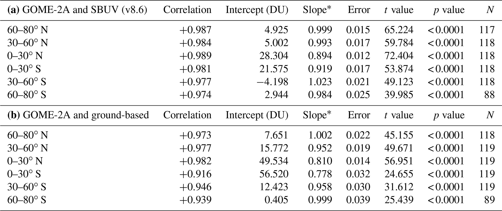
* Error, t value, and p value refer to slope.
Next, we studied the correlation between total ozone from GOME-2A and SBUV satellite data using linear regression analysis for the period 2007–2016. The statistical significance of the correlation coefficients, R, was calculated using the t-test formula for R with N−2 degrees of freedom, as used in Zerefos et al. (2018). The regression model showed statistically significant correlations between the different datasets as follows: in the tropics, mid-latitudes, and the northern high latitudes and in the southern high latitudes. All correlation coefficients are highly statically significant (99.9 % confidence level). In the long term, statistically significant correlation coefficients () are also found between GOME-2A satellite and GB measurements (Fig. 2), despite the different type of instruments used to measure total ozone from the ground. The regression parameters for the correlation coefficients shown in Figs. 1 and 2 are provided in Table 2.
A large part of the strong correlations shown in Figs. 1 and 2 is attributable to the seasonal variability of total ozone which is presented in Fig. 3 for GOME-2A, SBUV, and GB data. More specifically, Fig. 3 shows the seasonal variations of total ozone from station data, averaged from zones per 10∘ latitude, north and south. At high latitudes our analysis stops at 80∘. There is a very good agreement between the annual cycles of total ozone from the three datasets denoting the consistency of the satellite retrievals with GB observations. Similar annual cycles are also found with the GTO-ECV ozone data (not shown). Similar consistency is also revealed for the amplitudes of the annual cycles, computed as (maximum value – minimum value)/2 in Dobson units (DU). Figure 4 shows global maps of the amplitude of the annual cycle of total ozone for the period 2007–2016 from GOME-2A (panel a), GTO-ECV (panel b), and the TOMS–OMI–OMPS (panel c) satellite data. All maps are plotted against the sine of the latitude north and south in order to show areas according to their actual size. As can be seen from Fig. 4, the amplitude of the annual cycle is less than 20 DU in the tropics, increasing as we move towards the mid-latitudes and high latitudes to up to 75 DU. Interestingly, there is a region with small amplitude of the annual cycle in the southern mid-latitudes with values of about 10–15 DU, seen in Fig. 4 as a blue curved line crossing the longitudes around 60∘ S, which points to small seasonal variations of total ozone in these parts. The seasonal increase in Antarctic ozone is delayed by 2–3 months compared to the northern polar region. Only with the breakdown of the polar vortex in late spring, i.e. at a time when the poleward transport over lower latitudes has already ceased, does a strong ozone influx occur in the Antarctic. With this delay the amplitude of the seasonal variation stays much smaller poleward of 55–60∘ in the south than in the north (Dütsch, 1974). These features are consistent between all examined satellite datasets and are reproduced to a large extent by the Oslo CTM3 model as well, except in the southern mid-latitudes, where the model seems to underestimate the observed annual cycle (Fig. 4, panel d).
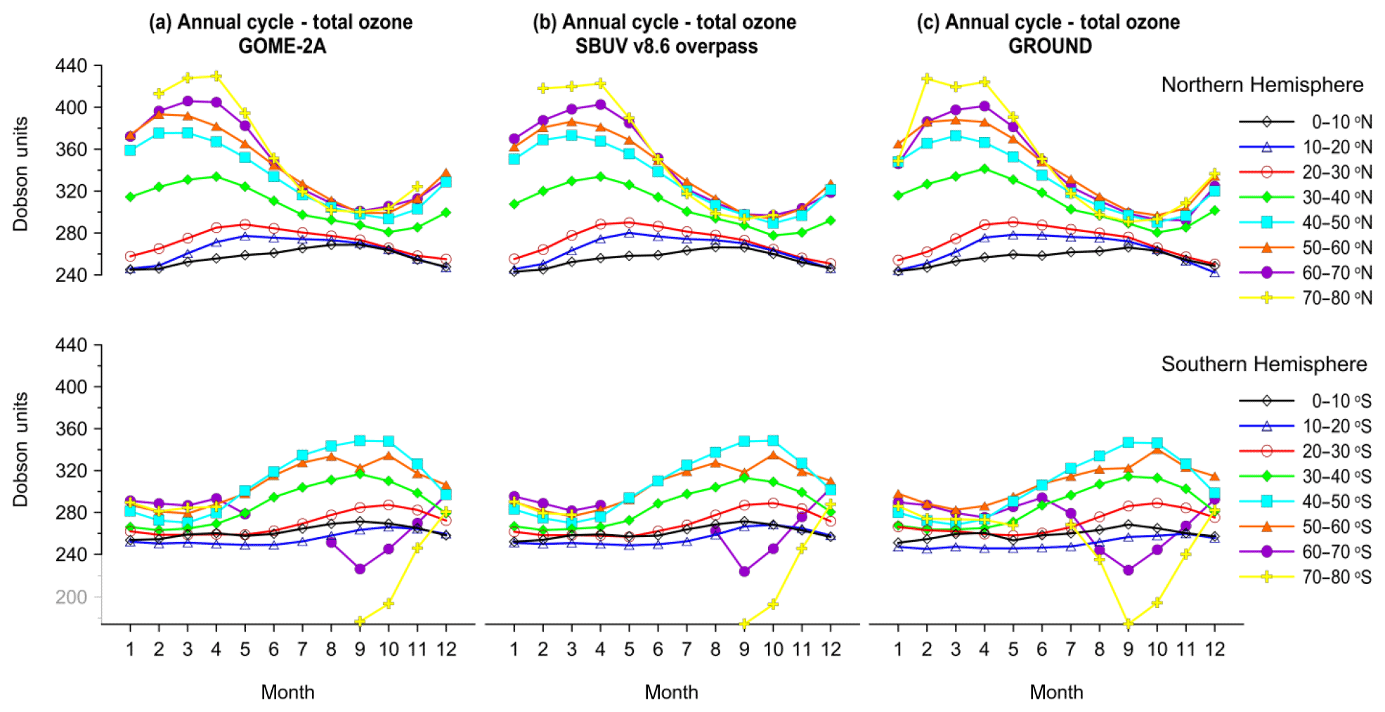
Figure 3Comparison of the annual cycle of total ozone from GOME-2A with that from SBUV (v8.6) satellite overpass data and GB observations in the period 2007–2016 based on station data averaged per 10∘ latitude zones. The annual cycle is distorted above 60∘ S due to the Antarctic ozone hole.
In summary, we find a similar pattern and amplitude of the annual cycle between total ozone from GOME-2A and the other examined total ozone datasets. The mean differences in the annual cycles of GOME-2A and SBUV satellite data are small in the tropics (0–30∘: 0.3±2.4 DU) and increase as we move towards the mid-latitudes (30–60∘: 2.4±4.4 DU) and higher latitudes (60–80∘: 1.7±4.8 DU). These numbers are consistent with the ones found between GOME-2A and GB measurements (tropics: 1.1±2.3 DU; mid-latitudes: 1.2±5.1 DU; high latitudes: 5.1±7.1 DU). In all latitude zones the correlation coefficients between the annual cycles of GOME-2A–SBUV and GOME-2A–GB data pairs were found to be greater than 0.9.
Before examining correlations with the large-scale natural fluctuations QBO, ENSO, and NAO, the mean annual cycle has been removed from the ozone datasets as described in the next section.
3.2 Correlation with QBO
We then studied how changes in dynamics affect the ozone columns in the atmosphere. The time series obtained have been deseasonalized by subtracting the long-term monthly mean from each individual monthly mean value. Ozone column variations for different latitude zones in the Northern and Southern Hemispheres have been compared. Figure 5 compares total ozone deseasonalized anomalies (in % of the mean) from GOME-2A and SBUV satellite retrievals in the tropics (10∘ N–10∘ S), subtropics (10∘–30∘ N and 10∘–30∘ S), and mid-latitudes (30∘–60∘ N and 30∘–60∘ S). The right panel of Fig. 5 shows the respective anomalies from GTO-ECV data. Mean differences between GOME-2A and SBUV deseasonalized monthly zonal means between 60∘ N and 60∘ S are less than ±0.5 %.
The dotted line superimposed on the ozone anomalies in Fig. 5 shows the equatorial zonal winds at 30 hPa, which were used as a proxy index to study the impact of QBO on total ozone. The general features include a QBO signal in total ozone at latitudes between 10∘ N and 10∘ S, which almost matches with the phase of QBO in the zonal winds. At higher northern and southern latitudes there is a phase shift in the QBO impact on total ozone. The impact of QBO is most pronounced in the tropics and is less pronounced in the subtropics and mid-latitudes. Strong positive correlations with the QBO are found in the tropics (correlation between GOME-2A and the QBO is about +0.77, t test =12.91) and weaker (usually of the opposite sign), less significant correlations are found at higher latitudes (about −0.15 in the northern extratropics and about −0.45 in the southern extratropics). Similar correlation patterns with the QBO are found for the GTO-ECV, SBUV, and GB data. These correlations suggest that the variability that can be attributed to the QBO in the tropics is about 60 % and is about 2 % and 20 % in the northern and the southern extratropics, respectively.
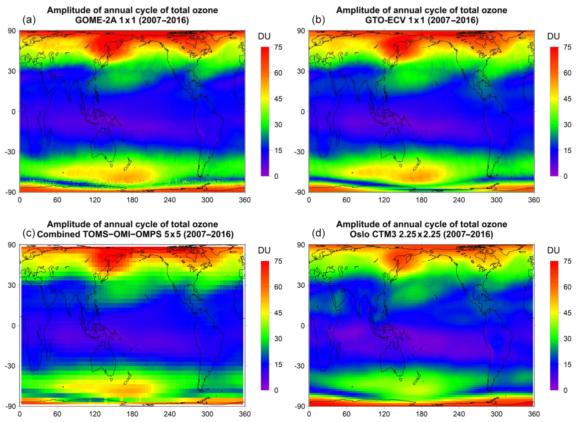
Figure 4Comparison of the amplitude, i.e. (maximum value – minimum value)/2, of the annual cycle of total ozone from GOME-2A (a) with the amplitude of the annual cycle of total ozone from GTO-ECV (b), the combined TOMS–OMI–OMPS satellite data (c), and Oslo CTM3 model simulations (d).
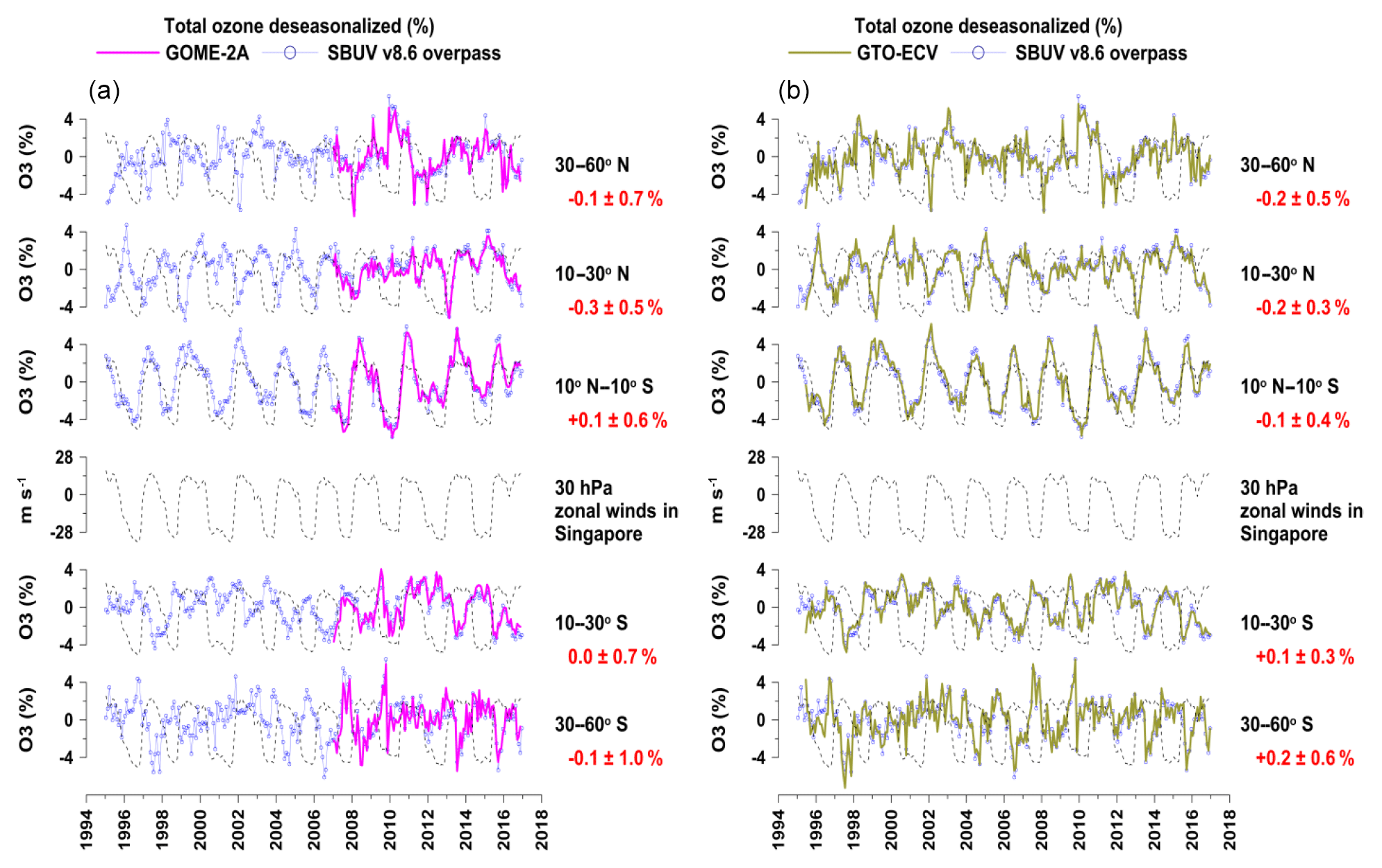
Figure 5(a) Time series of deseasonalized total ozone from GOME-2A and SBUV (v8.6) satellite overpasses over different latitude zones, along with the equatorial zonal winds at 30 hPa as an index of the QBO; (b) same as in (a), but for GTO-ECV and SBUV. Values with red colour refer to the mean differences ±σ (in %) between GOME-2A and SBUV deseasonalized data averaged over various WOUDC stations (150 stations in the northern mid-latitudes – 30–60∘ N; 21 stations in the northern subtropics – 10–30∘ N; eight stations in the tropics – 10∘ S–10∘ N; 10 stations in southern subtropics – 10–30∘ S; and 12 stations in the southern mid-latitudes – 30–60∘ S). The QBO proxy is superimposed on the ozone anomalies.
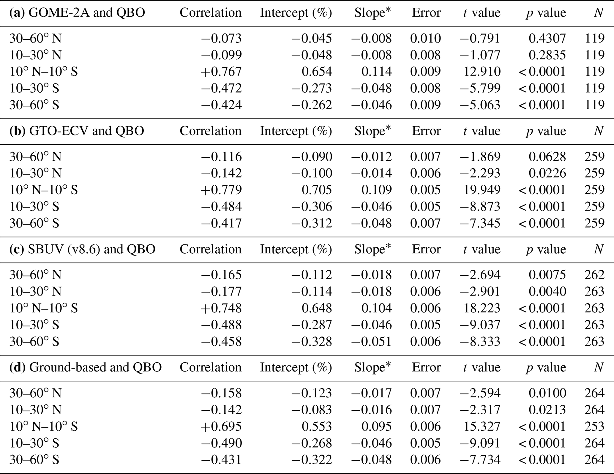
Table 3Statistics of correlations between deseasonalized total ozone and the QBO at 30 hPa for (a) GOME-2A data, (b) GTO-ECV data, (c) SBUV (v8.6) overpass data, and (d) ground-based measurements.
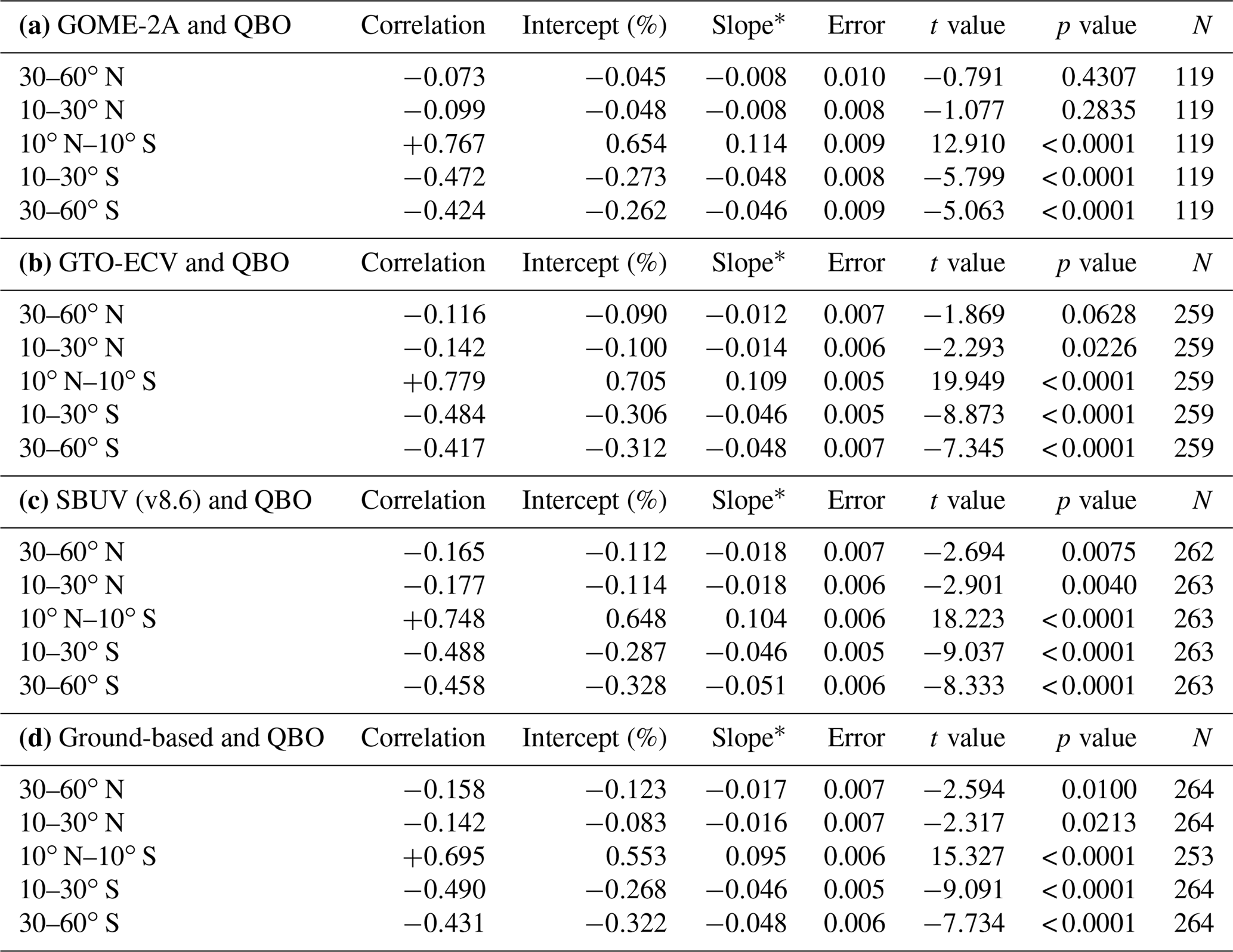
* The slope is in % per unit change of the explanatory variable. Error, t value, and p value refer to slope.
Table 3 summarizes the correlation and regression coefficients between total ozone and the QBO at 30 hPa for the different latitude zones and the different datasets. For latitudes between 10∘ N and 10∘ S correlations between total ozone from GOME-2A, GTO-ECV, SBUV, GB data, and the QBO are all positive. At latitudes between 10 and 30∘ the correlations turn to negative, in agreement with the results of Knibbe et al. (2014), who noted that when moving from the tropics towards higher latitudes, the regression estimates switch to negative values at approximately 10∘ N and 10∘ S. The correlations with the QBO at 30 hPa remain negative up to 60∘, a consistent result among all our datasets and something also reported by Knibbe et al. (2014) with the MSR ozone data. The correlation and regression coefficients between GOME-2A and the QBO are fairly similar to those found between SBUV and the QBO, as well as among all datasets as seen in Table 3, despite the different periods of records.

Figure 6Same as in Fig. 5, but for GOME-2A and GB observations (a) and for GTO-ECV and GB observations (b). The QBO proxy is superimposed on the ozone anomalies.
These features are also evident in Fig. 6, which compares GOME-2A (and GTO-ECV) satellite total ozone with GB observations with respect to the QBO. Mean differences and standard deviations between GOME-2A and GB and between GTO-ECV and GB deseasonalized total ozone data do not exceed 1 %. Again, correlation coefficients between deseasonalized GOME-2A and deseasonalized GB data are highly significant in all latitude zones (30–60∘ N, +0.91: slope =0.818, error =0.035, t value =23.466, and N=119; 10–30∘ N, +0.91: slope =0.786, error =0.033, t value =23.529, and N=119; 10∘ N–10∘ S, +0.94: slope =0.973, error =0.034, t value =28.449, and N=109; 10–30∘ S, +0.87: slope =0.864, error =0.044, t value =19.659, and N=119; 30–60∘ S, +0.88: slope =0.858, error =0.043, t value =19.854, and N=119). The same is true for the correlations between GTO-ECV and GB data pairs (30–60∘ N, +0.94; 10–30∘ N, +0.89; 10∘ N–10∘ S, +0.94; 10–30∘ S, +0.87; 30–60∘ S, +0.85). Our results are in line with Eleftheratos et al. (2013) and Isaksen et al. (2014), who compared QBO-related ozone column variations from the chemical transport model Oslo CTM2 with SBUV satellite data for shorter time periods. In summary, it has been shown that GOME-2A depicts the significant effects of QBO on stratospheric ozone in concurrence with SBUV and GB measurements. The instrument captures the variability of ozone in the tropics and the mid-latitudes correctly, which is nearly in phase with the QBO in the tropics and out of phase in the northern and the southern mid-latitudes, as has been shown by earlier studies (e.g. Zerefos, 1983; Baldwin et al., 2001).
3.3 Correlation with ENSO
Apart from the QBO, which affects the variability of total ozone in the tropics, an important mode of natural climate variability in the tropics is the ENSO. To examine the impact of the ENSO on total ozone in the tropics we first removed variability related to the QBO and the solar cycle and then performed the correlation analysis with the SOI. The effect of the QBO was removed from the time series by using a linear regression model for the total ozone variations at each grid box, of the form
where D(t) is the monthly deseasonalized total ozone and t is the time in months, with t=0 corresponding to the initial month and t=T corresponding to the last month. The term a0 is the intercept of the statistical model. To model the QBO we made use of the equatorial zonal winds at 30 hPa. The term a1 is the regression coefficient of the QBO. The QBO component was removed from the time series by using a phase lag with a maximum correlation of 28 months (month lag −14 to month lag 13). The QBO-related coefficients α0 and α1 of Eq. (1) for the deseasonalized GOME-2A, GTO-ECV, TOMS–OMI–OMPS, and Oslo CTM3 zonal mean data are presented in Table 3. Additional information for the regression coefficients α1 of QBO is provided in the Supplement Fig. S1, which shows the spatial distribution of the regression coefficients in latitude–longitude maps.
The residuals from Eq. (1) were then inserted in a second regression (Eq. 2) to account for the effect of the solar cycle on total ozone, as follows:
where β0 and β1 are now the intercept and regression coefficients of the solar cycle, respectively. To model the solar cycle we used the 10.7 cm wavelength solar radio flux (F10.7) as a proxy, taken from the National Research Council and Natural Resources Canada at ftp://ftp.geolab.nrcan.gc.ca/data/solar_flux/monthly_averages/solflux_monthly_average.txt (last access: 12 Decembe 2018). We use the absolute solar fluxes, which are adjusted to account for variations in Earth–Sun distance and uncertainty in antenna gain and waves reflected from the ground. Latitude–longitude maps of the regression coefficients β1 of the solar cycle are presented in the Fig. S2. We note that the global pattern of the regression coefficients of the solar cycle from GOME-2A data matches well with what has been shown by Knibbe et al. (2014) with the reanalysis MSR data.
The remainders from Eq. (2) were used in a third regression (Eq. 3) to study the correlations between total ozone and SOI at each individual grid box:
where c0 and c1 are now the intercept and regression coefficients of ENSO, respectively. Estimates of the regression coefficients c1 are shown in the Fig. S3.
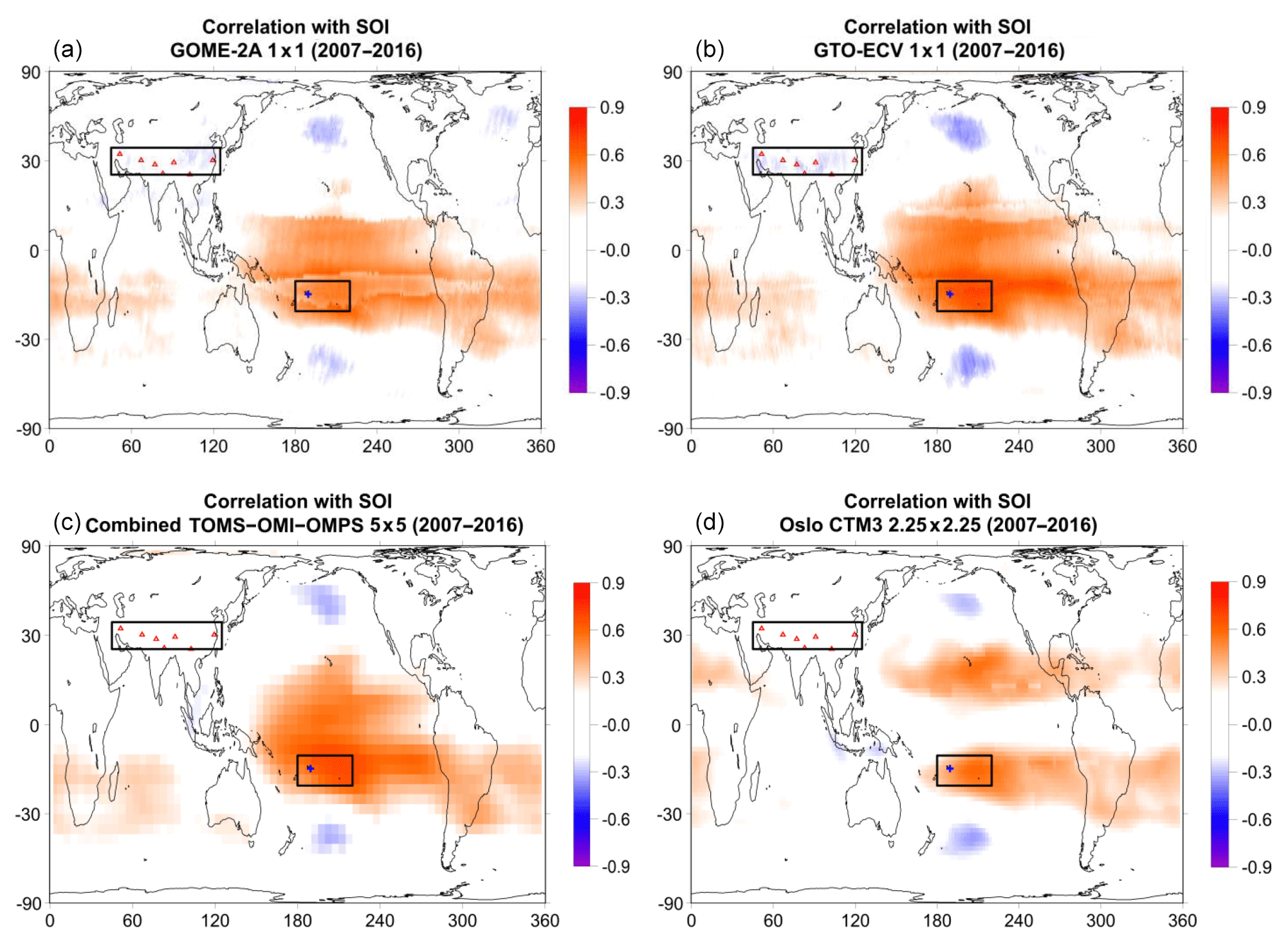
Figure 7Map of correlation coefficients between total ozone and SOI for GOME-2A (a), GTO-ECV (b), TOMS–OMI–OMPS satellite data (c), and Oslo CTM3 model simulations (d). Rectangles correspond to the southern Pacific region (10–20∘ S, 180–220∘ E) and southern Asia region (35–45∘ N, 45–125∘ E), blue cross corresponds to the Samoa station (14.25∘ S, 189.4∘ E), and red triangles correspond to stations in southern Asia, where total ozone has been studied as to the impact of ENSO after removing variability related to the annual cycle, QBO, and solar cycle. Positive correlations are shown in red colours, while negative correlations are shown in blue colours. Only correlation coefficients above or below ±0.2 are shown.
Figure 7 presents the correlations between the SOI and total ozone from GOME-2A (panel a), GTO-ECV (panel b), and TOMS–OMI–OMPS satellite data (panel c) as well as between the SOI and the Oslo model simulations (panel d). All four plots refer to the period 2007–2016. As can be seen from Fig. 7a, correlations of > 0.3 between GOME-2A total ozone and the SOI are found in the tropical Pacific Ocean at latitudes between 25∘ N and 25∘ S. These correlations were tested as to their statistical significance in the period 2007–2016, using the t test for R with N−2 degrees of freedom (as in Zerefos et al., 2018), and were found to be statistically significant. A similar picture of correlation coefficients is also observed by the GTO-ECV and TOMS–OMI–OMPS data. Both datasets show similar results as to the range of correlations (> 0.3) in the tropical Pacific for the common period of observations. Nevertheless, the spatial resolution is higher in the GOME-2A and GTO-ECV () data than in the TOMS–OMI–OMPS () data, so the former datasets perform better when looking at smaller space scales. We have to note here that in both maps there are larger areas with correlation coefficients > 0.3 in the southern part of the tropics than in the northern part. However, this was mostly observed during the period 2007–2016. By examining the longer-term data record of the TOMS–OMI–OMPS data, which extends back to 1979, we find symmetry in the pattern of correlations north and south of the Equator in the tropical Pacific Ocean (Fig. A1 of Appendix A), which indicates that both sides of the tropical Pacific are affected more or less in a similar way by El Niño–La Niña events. Finally, the Oslo CTM3 gives small correlations (< 0.3) in the tropical Pacific Ocean around the Equator, except over the northern and southern subtropics where the model compares better with the observations.
Table 4Annual mean total ozone, amplitude of annual cycle, amplitude of QBO, amplitude of solar cycle, and amplitude of ENSO in the period 1995–2016 from GOME-2A, GTO-ECV, the combined TOMS–OMI–OMPS satellite data, and Oslo CTM3 model calculations over the southern Pacific region (10–20∘ S, 180–220∘ E) and at the Samoa station (14.25∘ S, 189.4∘ E), located within this region.
* Period 2007–2016.
The small rectangle in Fig. 7 corresponds to the southern Pacific region (10–20∘ S, 180–220∘ E), and the blue cross corresponds to the Samoa station (American Samoa; 14.25∘ S, 189.4∘ E), where total ozone has been studied with respect to the impact of ENSO after removing the variability related to the annual cycle, QBO, and the solar cycle. Figure 8 shows an example of the ENSO impact on total ozone in the southern Pacific Ocean. Figure 8a shows the time series of total ozone anomalies from GOME-2A, GTO-ECV, and TOMS–OMI–OMPS satellite data together with the SOI. Comparisons of GOME-2A data with GTO-ECV data, SBUV overpass data, and GB measurements at the Samoa station are shown in Fig. 8b. The dotted line shows the respective tropopause pressure anomalies from the NCEP reanalysis. All datasets point to the strong influence of ENSO on total ozone. Most evident is the strong decrease of about 4 % in 1997–1998, which was caused by the strongest El Niño event in the examined period. A strong decrease is also observed in the tropopause pressures by NCEP. Also notable is the strong La Niña event in 2010 which caused total ozone to increase by about 4 %. We calculate a strong correlation between total ozone from GTO-ECV and the SOI of +0.66 (99 % confidence level), which accounts for about 40 % of the variability of total ozone over the tropical Pacific Ocean when the annual cycle, QBO signal, and solar cycle are removed. From the regression with SOI we estimated an ENSO-related term from which we calculated the amplitude of ENSO in total ozone as (maximum ozone – minimum ozone)/2. The amplitude of ENSO in total ozone was estimated to be 8.8 DU, or 3.5 % of the annual mean. This is comparable to the amplitude of the annual cycle (7.7 DU, or 3.0 % of the mean) and is larger than the amplitude of QBO (2.2 DU or 0.8 % of the mean) and the amplitude of the solar cycle in this region (4.1 DU, or 1.6 % of the mean). These results are based on the GTO-ECV total ozone data. Similar results were also found at the Samoa station from GB observations (i.e. correlation with SOI: +0.55; amplitude of ENSO: 7.7 DU, or 3.0 % of the mean; amplitude of the annual cycle: 6.7 DU, or 2.7 % of the mean). Statistics of total ozone such as mean, amplitude of the annual cycle, amplitude of the QBO, amplitude of the solar cycle, and amplitude of the ENSO in total ozone over the selected areas are presented in Table 4. Satellite, GB, and model data show consistent results. It also appears that the Samoa station represents the greater area in the southern Pacific well as to the impact of the ENSO.
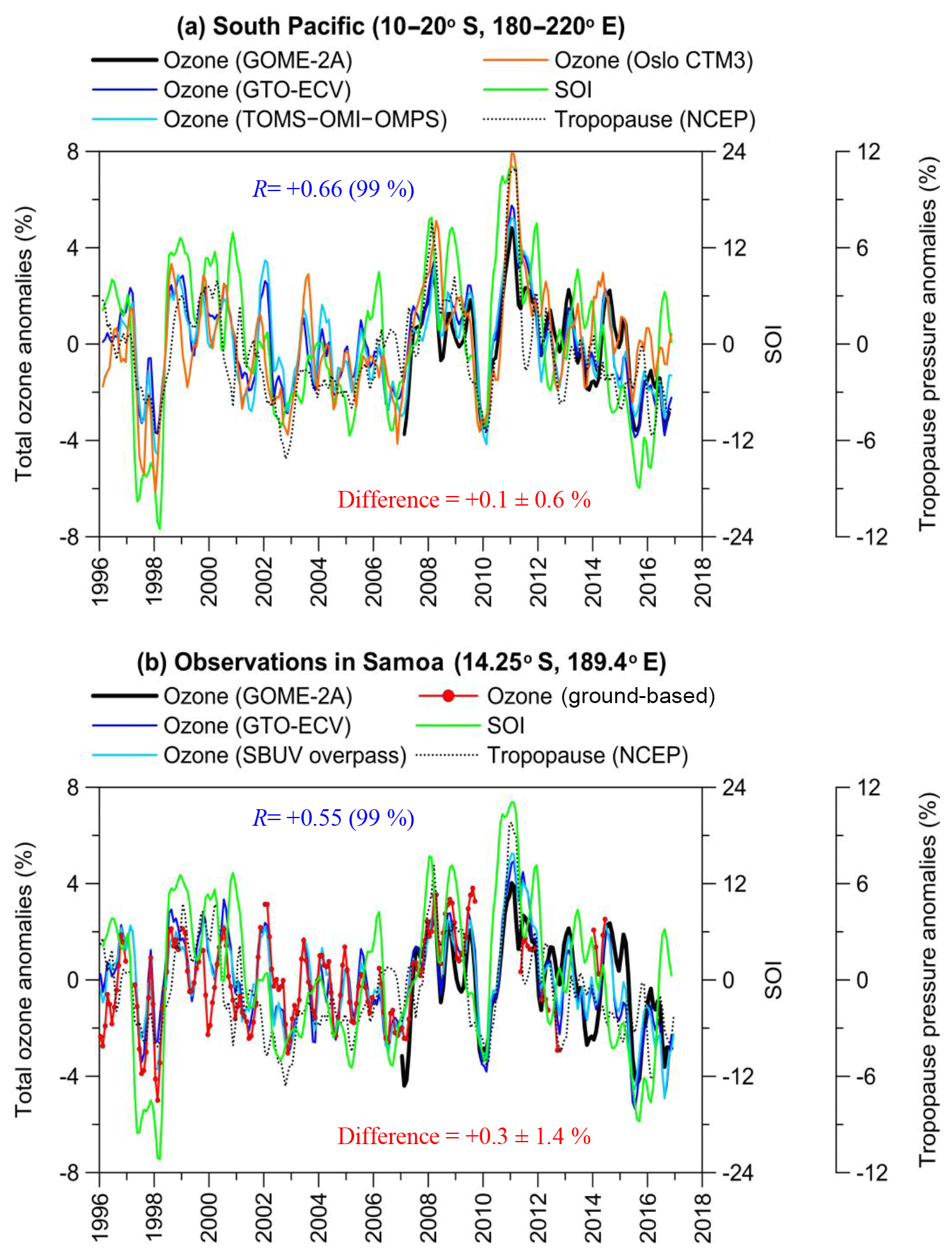
Figure 8(a) Example of regional time series of total ozone (%) over the southern Pacific region (10–20∘ S, 180–220∘ E) along with SOI. The dotted line shows the respective tropopause pressure variability from NCEP. R is the correlation coefficient between GTO-ECV total ozone and SOI (statistical significance of R is given in parentheses). The difference refers to the mean difference ±σ (in %) between GTO-ECV and the combined TOMS–OMI–OMPS satellite data; (b) same as in (a), but for SBUV overpass and GB data at the Samoa station. The difference refers to the mean difference ±σ (in %) between GTO-ECV and GB data.
Differences between GOME-2A and its data pairs in the southern Pacific Ocean are of the order of % between GOME-2A and TOMS–OMI–OMPS data, % between GOME-2A and GTO-ECV, and % between GOME-2A and Oslo CTM3. Accordingly, differences in Samoa are % between GOME-2A and GB data, 0.0±1.4 % between GOME-2A and GTO-ECV, and % between GOME-2A and SBUV. Despite the small differences found, we note here that GOME-2A values in the last 4 years of Figs. 8 and 9 slightly deviate from the other datasets and correlate weaker with the SOI than the other years in the time series. For instance, we estimate a drop in the correlation coefficient between GOME-2A and the SOI at the Samoa station (+0.58 in the period 2007–2012 and +0.47 in the period 2007–2016), which nevertheless does not alter the statistical significance of the correlation.
From Fig. 8 it also appears that there are high correlations with the tropopause height. The correlation coefficient between the NCEP tropopause pressure and GOME-2A total ozone over the southern Pacific Ocean is of the order of +0.59 (Student's t-test statistic results: t value =7.946, p value < 0.0001, and N=119). Accordingly, the correlation with GTO-ECV ozone data is of the order of +0.64 (t value =13.165, p value < 0.0001, and N=252), and with TOMS–OMI–OMPS, it is of the order of +0.58 (t value =10.913, p value < 0.0001, and N=241). The high correlation between the tropopause pressure and total ozone on interannual and longer time scales points to the very strong link between these parameters. These links were already documented in the past (e.g. Steinbrecht et al., 1998, 2001) and are verified with the GOME-2A data. At the same time a strong correlation is also evident between tropopause pressure and the SOI, again on interannual and longer time scales (, t value =13.825, p value < 0.0001, N=252). The above results point to the strong impact of the ENSO on the tropical ozone column through the tropical tropopause; warm (El Niño) and cold (La Niña) events affect the variability of the tropopause, which in turn affects the distribution of stratospheric ozone. In the tropics, where total ozone is mainly stratospheric, as the tropopause moves to higher altitudes (lower pressure), the stratosphere is compressed, reducing the amount of stratospheric (total) ozone. This happens during warm (El Niño) episodes. The opposite phenomenon occurs during cold (La Niña) events, when the tropopause height decreases (higher pressure) and total ozone is then increased. These events can affect the long-term ozone trends in the tropics when looking at time periods when strong El Niño and La Niña events occur at the beginning and the end of the trend period respectively (Coldewey-Egbers et al., 2014).
Table 5Statistics of the comparisons between total ozone, tropopause pressures, and SOI for (a) southern Pacific (10–20∘ S, 180–220∘ E), (b) Samoa station (14.25∘ S, 189.4∘ E), (c) southern Asia (35–45∘ N, 45–125∘ E), and (d) seven stations in southern Asia.
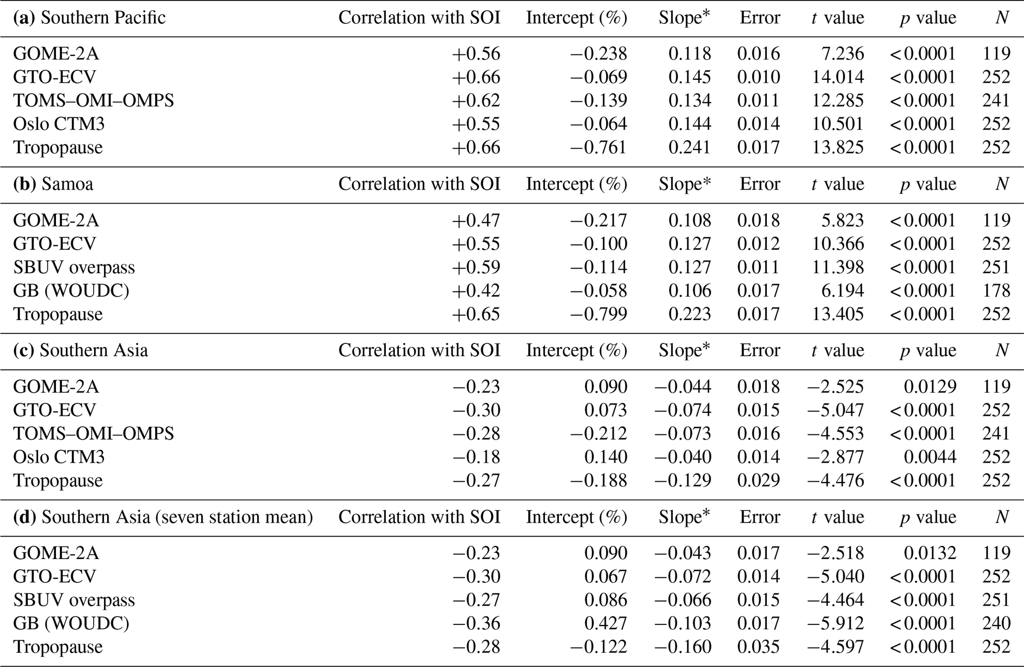
* The slope is in % per unit change of the explanatory variable. Error, t value, and p value refer to slope.

Figure 9(a) Example of regional time series of total ozone (%) over southern Asia (35–45∘ N, 45–125∘ E) along with SOI. The dotted line shows the respective tropopause pressure variability from NCEP. R is the correlation coefficient between GTO-ECV total ozone and SOI (statistical significance of R is given in parentheses). The difference refers to the mean difference ±σ (in %) between GTO-ECV and the combined TOMS–OMI–OMPS satellite data; (b) same as in (a) but with SBUV overpass and GB data averaged at seven stations in southern Asia. The difference refers to the mean difference ±σ (in %) between GTO-ECV and GB data.
Furthermore, in Fig. 8 we have marked seven stations in the greater southern Asia region (35–45∘ N, 45–125∘ E), where total ozone is anti-correlated with the SOI. Admittedly, these anti-correlations are weak (about −0.3), but we thought presenting the time series in these areas to be worthwhile as well. Figure 9 shows the variability of total ozone after removing seasonal, QBO, and solar-cycle-related variations, over the southern Asian region (panel a) and over the seven stations averaged within this region (panel b). As can be seen from this figure, the explained variance from the ENSO is small, not exceeding 9 %. All correlations from the comparisons with the SOI are summarized in Table 5. In spite of the small correlations with the SOI, the consistency between GOME-2A, GTO-ECV, TOMS–OMI–OMPS, and Oslo CTM3 data anomalies is very high, and their differences are within ±1 %. Differences at the seven stations in southern Asia are as follows: % between GOME-2A and GB data, % between GOME-2A and GTO-ECV, and % between GOME-2A and SBUV.
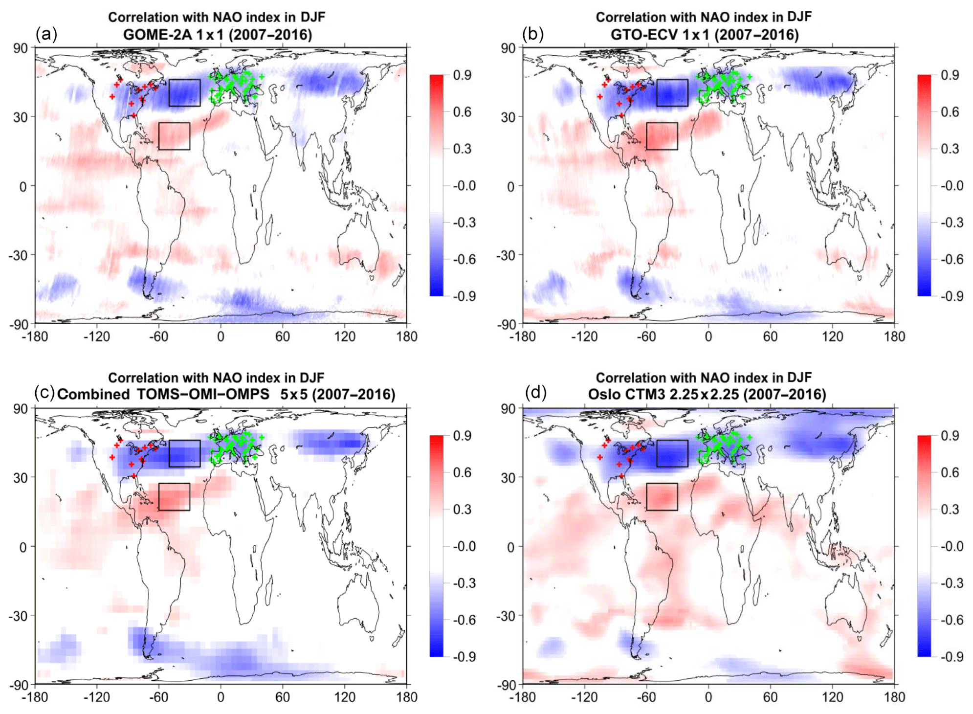
Figure 10Map of correlation coefficients between total ozone and the NAO index during winter (December, January, and February; DJF) for GOME-2A (a), GTO-ECV (b), TOMS–OMI–OMPS satellite data (c), and Oslo CTM3 model simulations (d). Rectangles correspond to regions in the North Atlantic (35–50∘ N, 20–50∘ W; 15–27∘ N, 30–60∘ W), and red and green crosses correspond to stations in Canada and USA and Europe, where total ozone has been studied as to the impact of NAO after removing variability related to the annual cycle, QBO, solar cycle, and ENSO. Positive correlations are shown by red colours, while negative correlations are shown by blue colours. Only correlation coefficients above or below ±0.2 are shown.
In summary, our findings indicate that GOME-2A captures the disturbances in total ozone during ENSO events well with respect to satellite SBUV and GB observations. Our findings on the ENSO-related total ozone variations (low ozone during ENSO warm events, high ozone during ENSO cold events, and magnitude of changes) are in line with recent studies (e.g. Randel and Thompson, 2011; Oman et al., 2013; Sioris et al., 2014) included in the 2014 Ozone Assessment report (Pawson and Steinbrecht, 2014; WMO, 2014). Our results are also in agreement with Knibbe et al. (2014), who showed negative ozone effects of El Niño between 25∘ S and 25∘ N, especially over the Pacific.
3.4 Correlation with NAO
The residuals from Eq. (3), free from seasonal, QBO, solar, and ENSO-related variations, were later used to study the correlation between total ozone and the NAO in winter. The results are presented in Fig. 10 which shows the correlation coefficients between total ozone and the NAO index in winter from the GOME-2A (panel a), GTO-ECV (panel b) and TOMS–OMI–OMPS satellite data (panel c), and the Oslo CTM3 model calculations (panel d). Negative correlations between total ozone and the NAO are presented with blue colours, while positive correlations are presented with red colours. From Fig. 10a it appears that total ozone is strongly correlated with the NAO in many regions. Strong negative correlation coefficients are observed in the majority of the northern mid-latitudes (R about −0.6), while positive correlations exist in the tropics and some negative correlations exist in the southern mid-latitudes. These characteristics are observed in both GTO-ECV and TOMS–OMI–OMPS datasets and are reproduced by the Oslo model as well, all for the common period 2007–2016. The regression coefficients on these comparisons are presented in the Fig. S4.
We note here that the results of the correlation analysis for the period 2007–2016 were based on a relative small sample of data from 10 winters, therefore many of these correlation coefficients may not be statistically significant. The statistical significance of the correlation coefficients in every grid box was only tested with the TOMS–OMI–OMPS data (Fig. A2, Appendix A), which provided us with the opportunity to calculate the respective correlations using data for the whole period of record 1979–2016. It appears that when extending the data back to the 1980s, the negative correlations in the southern mid-latitudes in winter disappear while the positive correlations in the tropics become weaker; yet the observed anti-correlation between total ozone and the NAO index in the northern mid-latitude zone remains strong. The dotted line in the plot shows areas with statistically significant correlation coefficients (99 % confidence level). Indeed, in the long term, statistically significant correlations between total ozone and the NAO index during winter are mostly found over the northern mid-latitudes and the subtropics. A small, statistically significant signal is also seen over Antarctica, but it was not analysed further.
According to this finding, we have restricted the analysis of the NAO to the northern mid-latitudes. Rectangles (Fig. 10a) correspond to two regions in the North Atlantic, i.e. 35–50∘ N, 20–50∘ W and 15–27∘ N, 30–60∘ W, which were studied for the impact of the NAO on total ozone after removing variability related to the annual cycle, QBO, solar cycle, and ENSO. In addition we have studied a number of stations in Canada, USA, and Europe that contribute ozone data to WOUDC, which are marked by red and green crosses in Fig. 10. The red crosses refer to the monitoring stations in Canada and the US, and the green crosses refer to the stations in Europe. In Fig. 11 we present the times series of total ozone anomalies from GOME-2A, GTO-ECV, and TOMS–OMI–OMPS satellite data along with the NAO index in winter over the North Atlantic. Model calculations are shown as well. The dotted line shows the respective tropopause pressure anomalies from NCEP reanalysis. Comparisons between GOME-2A, GTO-ECV, SBUV (v8.6) overpass data, and GB measurements over the various stations in Canada, USA, and Europe are shown in Fig. 12.
The observed anomalies over the North Atlantic Ocean point to the strong influence of the NAO on total ozone in winter. Most evident is the strong increase in total ozone in 2010 of more than 8 %, particularly over 35–50∘ N and 20–50∘ W. This increase was accompanied by a strong increase in tropopause pressures. Both changes (in total ozone and tropopause pressures) occurred under a strong negative phase of the NAO, the strongest one in the past 20 years. We observe strong anti-correlation among total ozone and the NAO index in winter ( over 35–50∘ N, 20–50∘ W), which is statistically significant at the 99 % confidence level. This anti-correlation suggests that about 50 % of the variability of total ozone in winter is explained by the NAO when the annual cycle, QBO, solar cycle, and ENSO signals are removed. Differences for GOME-2A, and its data pairs are estimated to be % between GOME-2A and TOMS–OMI–OMPS data, % between GOME-2A and GTO-ECV, and % between GOME-2A and Oslo CTM3 data. From the regression with the NAO index we derived an NAO-related term from which we calculated the amplitude of the NAO in total ozone as (maximum ozone – minimum ozone)/2. The amplitude of the NAO over the North Atlantic region (35–50∘ N, 20–50∘ W) was estimated to be about 16.5 DU, or 5.2 % of the annual mean. This is about half of the amplitude of the annual cycle (which is ∼37 DU or 11.7 % of the mean). These estimates are based on GTO-ECV data. Similar correlation and amplitude were also found with GOME-2A, the combined TOMS–OMI–OMPS satellite data, and the Oslo CTM3 model simulations.
Table 6Annual mean total ozone, amplitude of annual cycle, amplitude of QBO, amplitude of solar cycle, and amplitude of NAO in the period 1995–2016 from GOME-2A, GTO-ECV, the combined TOMS–OMI–OMPS satellite data, and Oslo CTM3 model calculations over the North Atlantic Ocean, in (a) region 35–50∘ N, 20–50∘ W, and (b) region 15–27∘ N, 30–60∘ W.
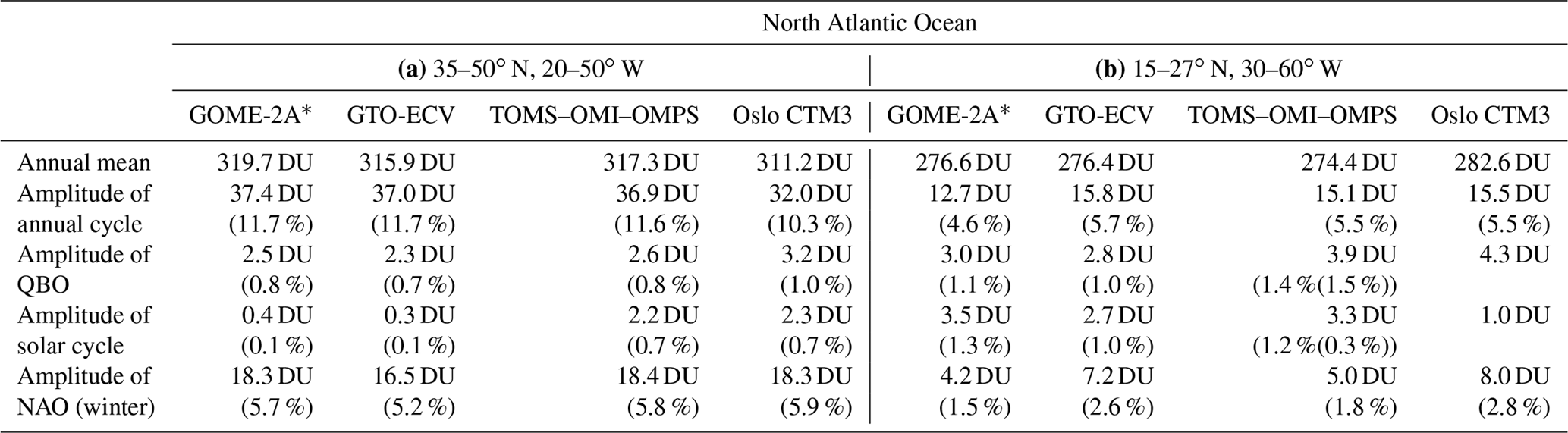
* Period 2007–2016.
A similar but opposite correlation is found over the southern part of the North Atlantic (15–27∘ N, 30–60∘ W). Here, we estimate a significant correlation coefficient of the NAO of +0.60, amplitude of the NAO of about 7.2 DU (2.6 % of the annual mean), and amplitude of the annual cycle of about 15.8 DU (5.7 % of the mean). Again, similar estimates are found with the GOME-2A and the TOMS–OMI–OMPS satellite data and are reproduced by the model calculations as well. The annual mean total ozone and the amplitudes of the annual cycle, QBO, solar cycle, and NAO in total ozone over the studied regions in the North Atlantic are summarized in Table 6. Differences between GOME-2A and GTO-ECV data at the southern part of North Atlantic are of the order of %. Differences with the TOMS–OMI–OMPS data are estimated to be % and are estimated to be % with the Oslo CTM3.
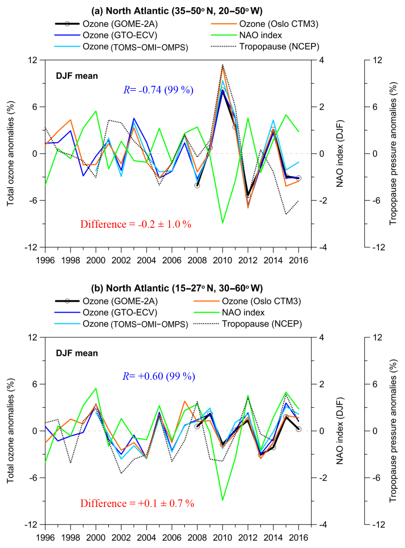
Figure 11Example of regional time series of total ozone (%) over the North Atlantic regions (a) 35–50∘ N, 20–50∘ W, and (b) 15–27∘ N, 30–60∘ W, in winter (DJF mean) along with the NAO index. The dotted line shows the respective tropopause pressure variability from NCEP reanalysis. R is the correlation coefficient between GTO-ECV total ozone and the NAO index. The differences refer to the mean differences ±σ (in %) between GTO-ECV and the combined TOMS–OMI–OMPS satellite data.
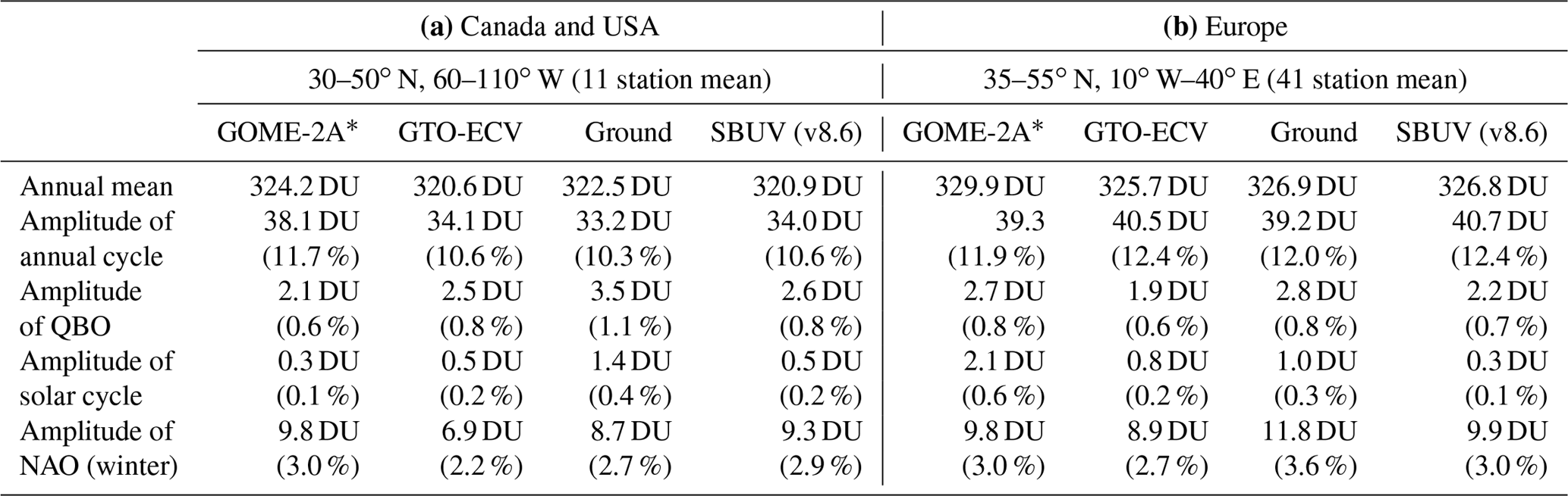
The time series of total ozone anomalies and of the NAO index for the examined stations in Canada, USA, and Europe are presented in Fig. 12. Table 7 presents the respective statistics. The correlation between total ozone and the NAO index in winter after removing ozone variability related to the annual cycle, QBO, solar cycle, and ENSO is −0.40 (90 % confidence level). Again, a particular feature was the total ozone increase in 2010 by 6 % of the mean associated with the negative NAO phase. This increase is noteworthy because of the consistency with the GB measurements and the satellite SBUV overpass data and, in general, the agreement found between the variability of the tropopause pressures and total ozone. Differences between GOME-2A and GB data are %. Accordingly we estimate differences of about % between GOME-2A and GTO-ECV data and of about % between GOME-2A and SBUV data. On the basis of GTO-ECV data we estimate that in Canada and the USA, the amplitude of the NAO in total ozone in winter is about 7 DU (or 2.2 % of the mean), while it is estimated to be about 9 DU (or 2.7 % of the mean) over Europe. These numbers are slightly smaller than the GOME-2A, GB, and SBUV estimates, less than about one percent (Table 7).
Table 7Annual mean total ozone, amplitude of annual cycle, amplitude of QBO, amplitude of solar cycle, and amplitude of NAO in the period 1995–2016 from GOME-2A, GTO-ECV satellite data, ground-based observations, and SBUV (v8.6) satellite overpass data over (a) Canada and USA (11 station mean) and (b) Europe (41 station mean).
* Period 2007–2016.
Table 8Statistics of the comparisons between total ozone, tropopause pressures, and NAO index in winter (DJF mean) for (a) the northern part of North Atlantic (35–50∘ N, 20–50∘ W), (b) its southern part (15–27∘ N, 30–60∘ W), (c) 11 stations in Canada and USA, and (d) 41 stations in Europe.
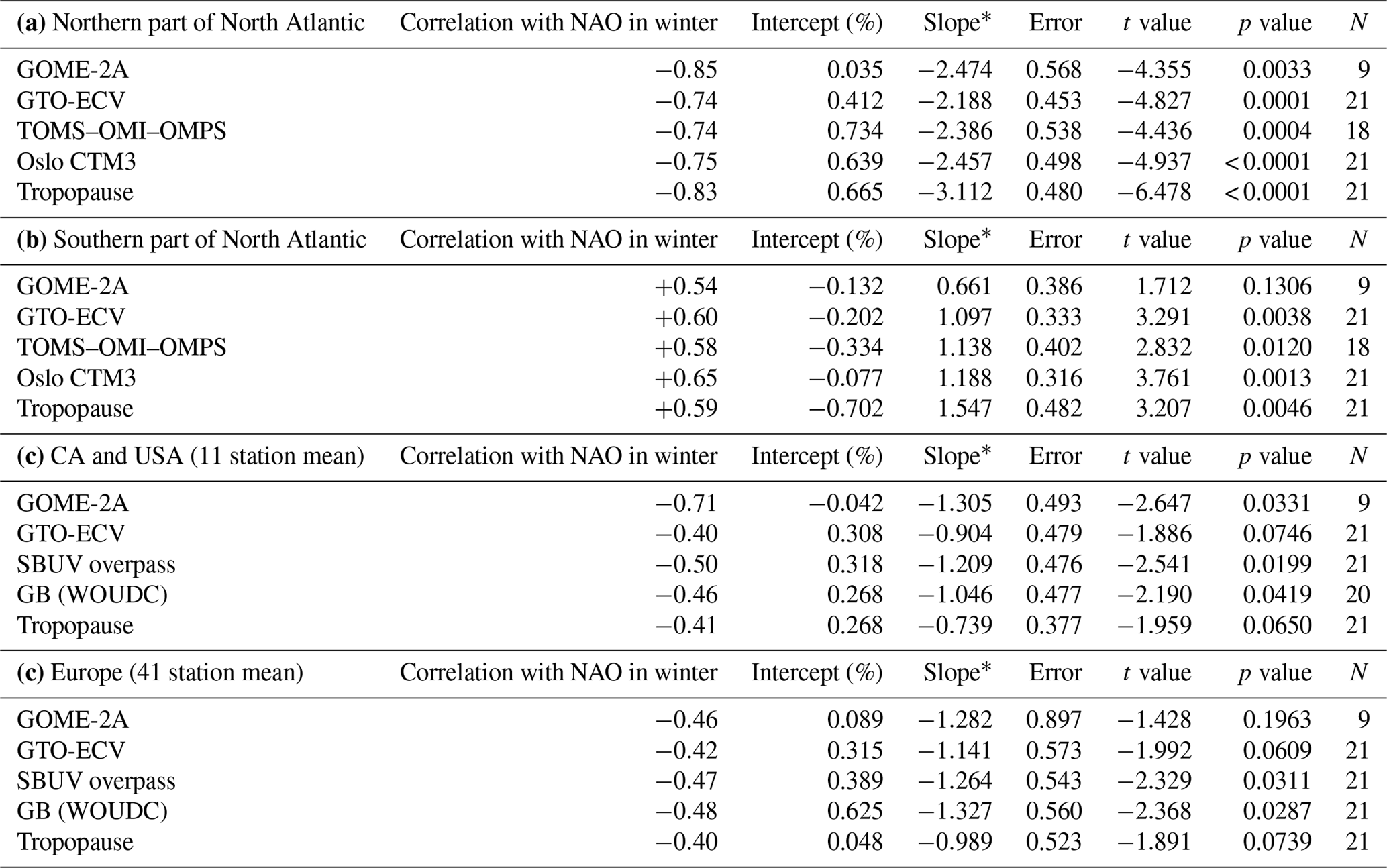
* The slope is in % per unit change of the explanatory variable. Error, t value, and p value refer to slope.
The anti-correlation between total ozone column and the NAO index during winter also applies to southern Europe and the Mediterranean. Following the study of Ossó et al. (2011), who reported a reversal in the correlation pattern between the NAO and total ozone from winter to summer in southern Europe, we have looked at the correlations during summer as well. Figure 13 presents the comparisons for 21 ground-based stations located in the region bounded by latitudes 30–47∘ N and by longitudes 10∘ W–40∘ E. Figure 13a shows results for the summer, and Fig. 13b shows results for the winter. As can be seen, the observed anti-correlation between GB total ozone and the NAO in winter (, slope , t value , p value =0.0499, and N=21) reverses its sign and becomes positive in the summer (, slope =0.874, t value =3.309, p value =0.0037, and N=21), indicating that the NAO explains about 36 % of ozone variability in the summer in this region. A similar picture is also seen from GOME-2A, GTO-ECV, and SBUV data.
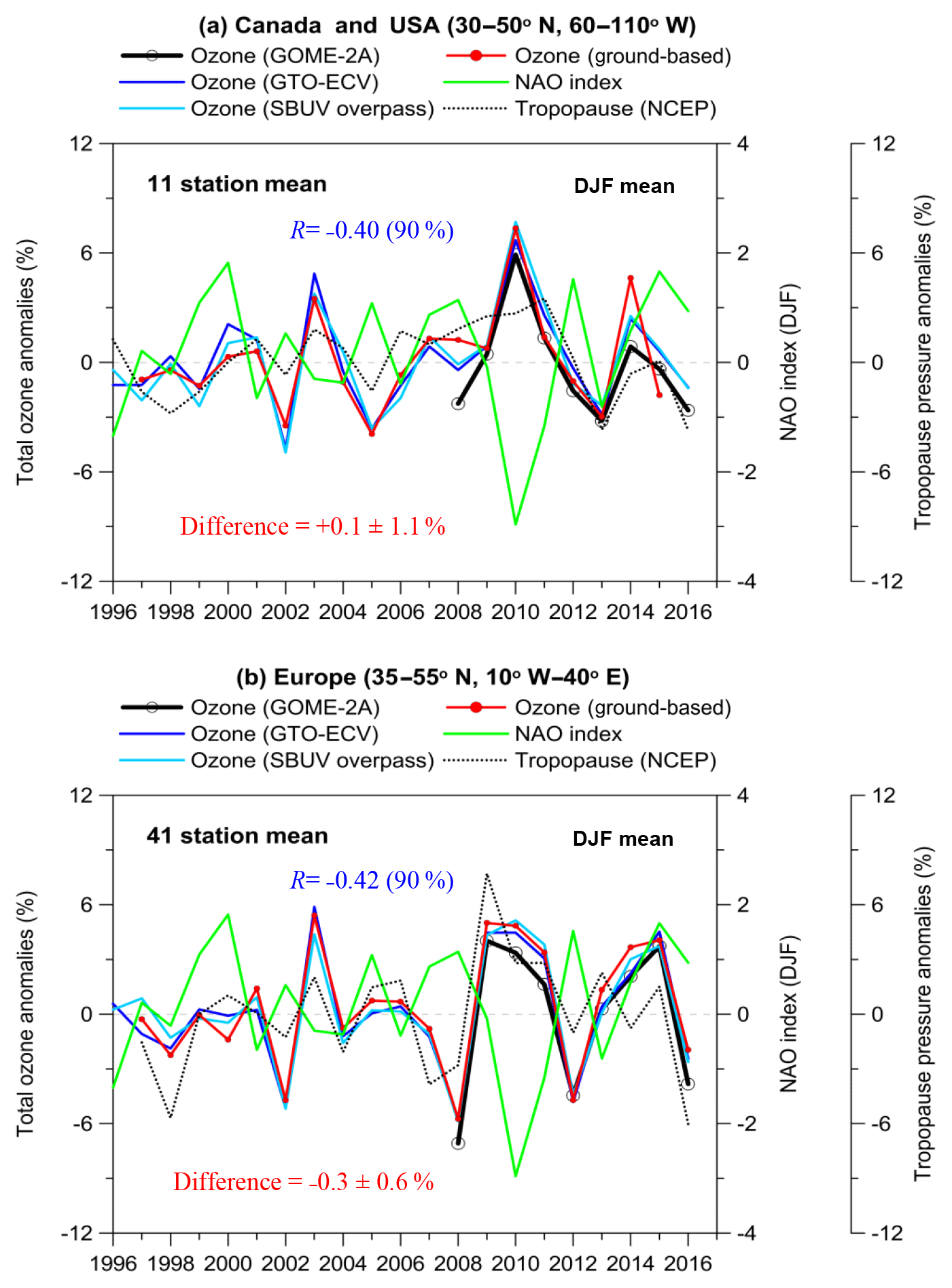
Figure 12Comparison with GB observations over (a) Canada and USA and (b) Europe in winter (DJF mean). R is the correlation coefficient between GTO-ECV total ozone and the NAO index. The differences refer to the mean differences ±σ (in %) between GTO-ECV and GB data.
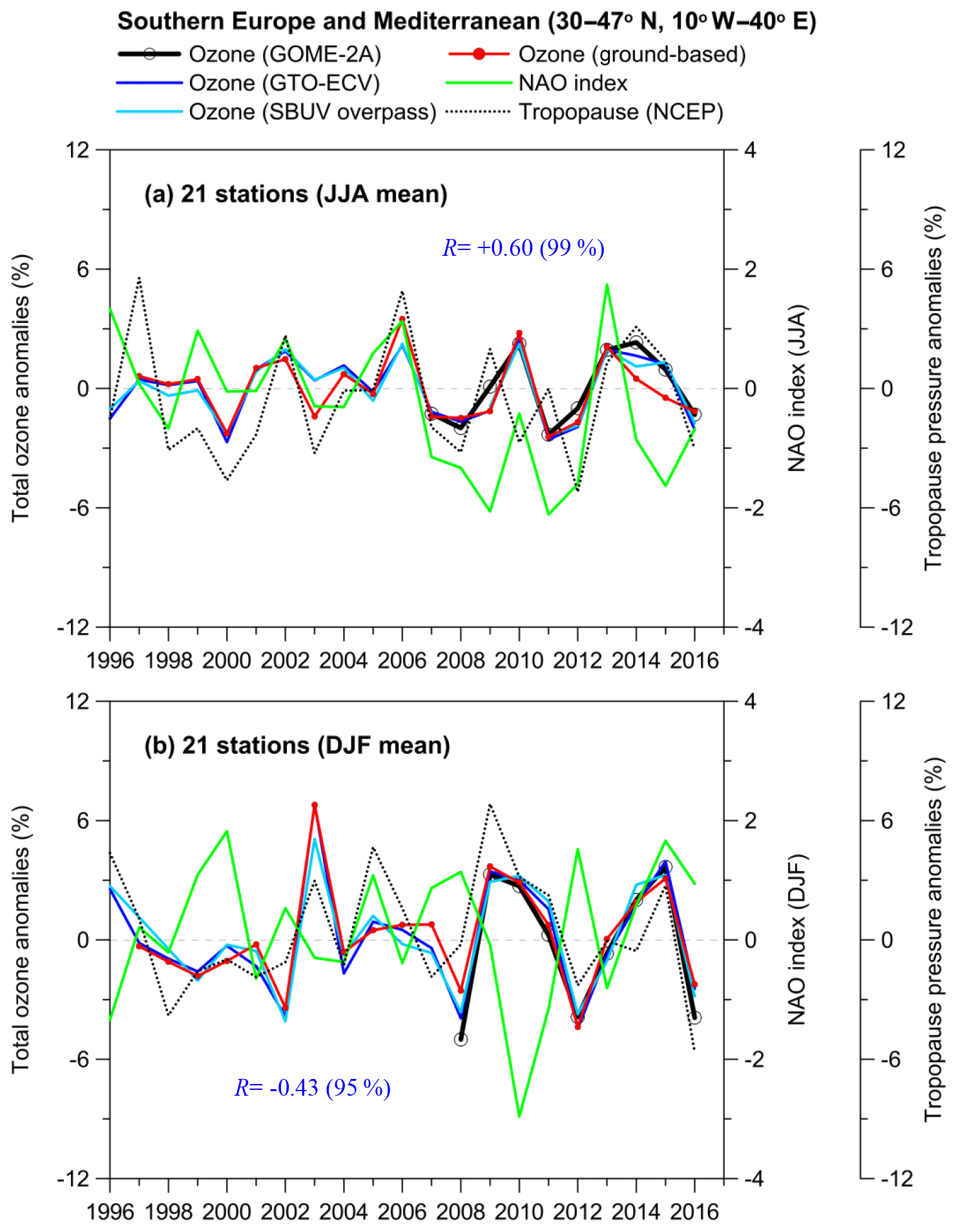
Figure 13Relation between total ozone and the NAO index in summer (JJA mean) and winter (DJF mean) for 21 stations in southern Europe. The correlation coefficients refer to NAO index and GB total ozone after removing variability related to the seasonal cycle, QBO, solar cycle, and ENSO.
In summary, our findings based on GOME-2A, GTO-ECV, and SBUV overpass data are in line with those found by Ossó et al. (2011) and Steinbrecht et al. (2011), who analysed TOMS and OMI satellite data and GB measurements at the Hohenpeißenberg station, respectively. During winter, total ozone variability associated with the NAO is particularly important over northern Europe, the US East Coast, and Canada, explaining up to 30 % of total ozone variance for this region (Ossó et al., 2011). Also, both studies found unusually high total ozone columns in 2010 over much of the Northern Hemisphere and related them to the negative phase of the NAO or AO (the Arctic Oscillation).
We have evaluated the ability of GOME-2–MetOp-A (GOME-2A) satellite total ozone retrievals to capture known natural oscillations such as the QBO, ENSO, and NAO. In general, GOME-2A depicts these natural oscillations in concurrence with GTO-ECV, TOMS–OMI–OMPS, and SBUV (v8.6) satellite overpass data; ground-based measurements (Brewer, Dobson, filter, and SAOZ); and chemical transport model calculations (Oslo CTM3).
Mean differences between GOME-2A and SBUV total ozone were found to be % in the tropics (0–30∘), about % in the mid-latitudes (30–60∘), about % over the northern high latitudes (60–80∘ N), and about % over the southern high latitudes (60–80∘ S). These differences were estimated as (GOME-2A – SBUV)/SBUV (%) from January 2007 to December 2016. Small differences were also found between GOME-2A and GB measurements, with standard deviations of the differences being ±1.4 % in the tropics, ±2.1 % in the mid-latitudes, and ±3.2 % and ±4.3 % over the northern and the southern high latitudes respectively.
The variability of total ozone from GOME-2A has been compared with the variability of total ozone from other examined datasets as to their agreement depicting natural atmospheric phenomena such as the QBO, ENSO, and NAO. First, we studied correlations between total ozone and the QBO after removing variability related to the seasonal cycle from the ozone datasets. Then, we examined correlations between total ozone and the ENSO after removing variability related to the QBO and the solar cycle, and we finally examined correlations with the NAO after removing variability related to the QBO, solar cycle, and ENSO. Our main results are as follows.
QBO. Total ozone from GOME-2A is well correlated with the quasi-biennial oscillation (+0.8 in the tropics) in agreement with GTO-ECV, SBUV, and GB data. The amplitude of the QBO on total ozone maximizes around the Equator, and it is estimated to be about 2.6 % of the mean. Going from low to mid-latitudes there is a phase shift in the QBO impact on total ozone. Correlation coefficients between GOME-2A total ozone and the QBO over 30–60∘ north and south are −0.1 and −0.5 respectively, in agreement with the correlations between GB total ozone and the QBO (−0.2 and −0.5, respectively). On the basis of GOME-2A, the amplitude of QBO in total ozone is estimated to be 0.6 % of the mean in the northern mid-latitudes and 1.4 % of the mean in the southern mid-latitudes.
ENSO. Correlation coefficients among GOME-2A total ozone and the SOI in the tropical Pacific Ocean are estimated to be about +0.6, consistent with GTO-ECV, SBUV, and GB observations. It was found that the El Niño–Southern Oscillation (ENSO) signal is evident and consistent in all examined datasets. The amplitude of ENSO in total ozone is about 6–9 DU, corresponding to about 2.5 %–3.5 % of the annual mean. Differences between GOME-2A, GTO-ECV, and GB measurements during warm (El Niño) and cold (La Niña) events are within ±1.5 %. Similar estimates also result from the Dobson measurements in American Samoa, indicating that the Samoa station represents the greater area in the southern Pacific well for satellite evaluations as to the impact of the ENSO.
NAO. The respective results related to the impact of the North Atlantic Oscillation over the northern mid-latitudes showed a clear NAO signal in winter in all datasets, with amplitudes of about 16–19 DU (about 5 %–6 % of the annual mean) in the North Atlantic, 9–12 DU (3 %–4 % of the mean) over Europe, and 7–10 DU (2 %–3 % of the mean) over Canada and the US. Comparison with GB observations over Canada and Europe showed very good agreement between GOME-2A, GTO-ECV, and GB observations as to the influence of the NAO, with differences within ±1 %.
In addition to the usual validation methods, which compare monthly mean and zonal mean total ozone data and analyse the differences between satellite and GB instruments, we showed here that quasi-cyclical perturbations such as the QBO, ENSO, and NAO can serve as independent proxies of spatiotemporal variation to qualitatively evaluate GOME-2A satellite total ozone against ground-based and other satellite total ozone datasets. The agreement and small differences which were found between the variability of total ozone from GOME-2A and the variability of total ozone from other satellite retrievals and ground-based measurements during these naturally occurring oscillations verify the good quality of GOME-2A satellite total ozone to be used in ozone–climate research studies.
Satellite SBUV (v8.6) total ozone station overpass data were downloaded from https://acd-ext.gsfc.nasa.gov/Data_services/merged/index.html (last access: 8 February 2019; McPeters et al., 2013; Bhartia et al., 2013). GTO-ECV total ozone data are available at http://www.esa-ozone-cci.org/?q=node/160 (last access: 8 February 2019; Coldewey-Egbers et al., 2015; Garane et al., 2018). Ground-based total ozone daily summaries were obtained from the World Ozone and Ultraviolet Radiation Data Centre (WOUDC) at https://doi.org/10.14287/10000001 (WOUDC, 2018). The QBO component of total ozone was examined by using the monthly mean zonal winds in Singapore at 30 hPa. Zonal wind data at 30 hPa were provided by the Freie Universität Berlin (FU-Berlin) at http://www.geo.fu-berlin.de/met/ag/strat/produkte/qbo/qbo.dat (last access: 8 February 2019; Naujokat, 1986). The Southern Oscillation Index (SOI) was provided by the Bureau of Meteorology of the Australian Government at http://www.bom.gov.au/climate/current/soi2.shtml (Australian Government – Bureau of Meteorology, 2018). The NAO index for December, January, and February was provided by the Climate Analysis Section of NCAR in Boulder, CO, USA at https://climatedataguide.ucar.edu/climate-data/hurrell-north-atlantic-oscillation-nao-index-pc-based (last access: 8 February 2019; Hurrell and Deser, 2009). The tropopause pressures from the NCEP/NCAR Reanalysis 1 dataset were downloaded from https://www.esrl.noaa.gov/psd/data/gridded/data.ncep.reanalysis.tropopause.html (last access: 8 February 2019; Kalnay et al., 1996).
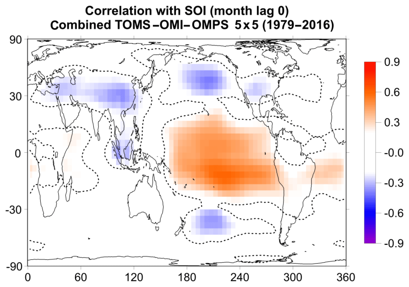
Figure A1Map of correlation coefficients between total ozone from TOMS–OMI–OMPS satellite data and SOI for the whole period 1979–2016, after removing variability related to the seasonal cycle, QBO, and solar cycle. The dotted line binds the regions where the correlation coefficients are statistically significant at the 99 % confidence level (t test). Only correlation coefficients above or below ±0.2 are shown. Ozone data for the period 1991–1993 after the Mt Pinatubo eruption were not used in the correlation analysis to avoid any data contamination by the volcanic aerosols.
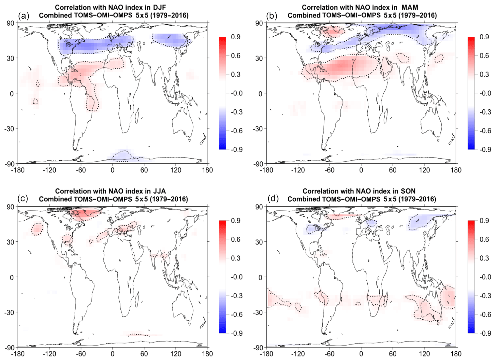
Figure A2Map of correlation coefficients between total ozone from TOMS–OMI–OMPS satellite data and the NAO index during winter (December, January, and February – DJF; a), spring (March, April, amd May – MAM; b), summer (June, July, and August – JJA; c), and autumn (September, October, and November – SON; d) for the whole period 1979–2016, after removing variability related to the seasonal cycle, QBO, solar cycle, and ENSO. The dotted line binds the regions where the correlation coefficients are statistically significant at the 99 % confidence level (t test). Only correlation coefficients above or below ±0.2 are shown. Ozone data for the period 1991–1993 after the Mt Pinatubo eruption were not used in the correlation analysis to avoid any data contamination by the volcanic aerosols.
The supplement related to this article is available online at: https://doi.org/10.5194/amt-12-987-2019-supplement.
KE prepared the paper based on contributions from all co-authors. CZ, DB, and MEK evaluated the results. MCE, DL, PV, CL, and SH processed GOME-2A satellite data. JK processed ground-based data. SF processed TOMS-OMI-OMPS and SBUV-2 satellite data. AH and ISAI processed Oslo CTM3 model data.
The authors declare that they have no conflict of interest.
Development of the GOME-2 and MetOp A total ozone products and their validation
have been funded by the AC SAF project with EUMETSAT and national
contributions. We acknowledge support of this work by the project
“PANhellenic infrastructure for Atmospheric Composition and climatE
chAnge” (MIS 5021516), which is implemented under the initiative “Reinforcement
of the Research and Innovation Infrastructure”, funded by the operational
programme “Competitiveness, Entrepreneurship and Innovation” (NSRF
2014–2020), and co-financed by Greece and the European Union (European
Regional Development Fund). We further acknowledge the
Mariolopoulos-Kanaginis Foundation for the Environmental Sciences, the ESA
Ozone CCI project, and the NASA Goddard Space Flight Center. The ground-based
data used in this publication were obtained as part of WMO's Global
Atmosphere Watch (GAW) and are publicly available via the World Ozone and
Ultraviolet Radiation Data Centre (WOUDC). The authors would like to thank all the
scientists that provide quality-assured total ozone column data on a timely basis to
the WOUDC database. We acknowledge the National Oceanic and Atmospheric
Administration (NOAA) for maintaining the American Samoa Dobson station. Kostas Eleftheratos
and Christos S. Zerefos would like to dedicate the study to the memory of Ivar Isaksen (University of Oslo), who passed away on 16 May 2017.
Edited by: Piet Stammes
Reviewed by: two anonymous referees
Australian Government – Bureau of Meteorology: Southern Oscillation Index (SOI) since 1986, available at: http://www.bom.gov.au/climate/current/soi2.shtml, last access: 15 June 2018.
Baldwin, M. P., Gray, L. J., Dunkerton, T. J., Hamilton, K., Haynes, P. H., Randel, W. J., Holton, J. R., Alexander, M. J., Hirota, I., Horinouchi, T., Jones, D. B. A., Kinnersley, J. S., Marquardt, C., Sato, K., and Takahashi, M.: The quasi-biennial oscillation, Rev. Geophys., 39, 179–229, https://doi.org/10.1029/1999RG000073, 2001.
Bhartia, P. K., McPeters, R. D., Flynn, L. E., Taylor, S., Kramarova, N. A., Frith, S., Fisher, B., and DeLand, M.: Solar Backscatter UV (SBUV) total ozone and profile algorithm, Atmos. Meas. Tech., 6, 2533–2548, https://doi.org/10.5194/amt-6-2533-2013, 2013.
Brönnimann, S., Bhend, J., Franke, J., Flückiger, S., Fischer, A. M., Bleisch, R., Bodeker, G., Hassler, B., Rozanov, E., and Schraner, M.: A global historical ozone data set and prominent features of stratospheric variability prior to 1979, Atmos. Chem. Phys., 13, 9623–9639, https://doi.org/10.5194/acp-13-9623-2013, 2013.
Chehade, W., Weber, M., and Burrows, J. P.: Total ozone trends and variability during 1979–2012 from merged data sets of various satellites, Atmos. Chem. Phys., 14, 7059–7074, https://doi.org/10.5194/acp-14-7059-2014, 2014.
Chiou, E. W., Bhartia, P. K., McPeters, R. D., Loyola, D. G., Coldewey-Egbers, M., Fioletov, V. E., Van Roozendael, M., Spurr, R., Lerot, C., and Frith, S. M.: Comparison of profile total ozone from SBUV (v8.6) with GOME-type and ground-based total ozone for a 16-year period (1996 to 2011), Atmos. Meas. Tech., 7, 1681–1692, https://doi.org/10.5194/amt-7-1681-2014, 2014.
Coldewey-Egbers, M., Loyola R., D. G., Braesicke, P., Dameris, M., van Roozendael, M., Lerot, C., and W. Zimmer, W.: A new health check of the ozone layer at global and regional scales, Geophys. Res. Lett., 41, 4363–4372, https://doi.org/10.1002/2014GL060212, 2014.
Coldewey-Egbers, M., Loyola, D. G., Koukouli, M., Balis, D., Lambert, J.-C., Verhoelst, T., Granville, J., van Roozendael, M., Lerot, C., Spurr, R., Frith, S. M., and Zehner, C.: The GOME-type Total Ozone Essential Climate Variable (GTO-ECV) data record from the ESA Climate Change Initiative, Atmos. Meas. Tech., 8, 3923–3940, https://doi.org/10.5194/amt-8-3923-2015, 2015 (data available at: http://www.esa-ozone-cci.org/?q=node/160, last access: 8 February 2019).
Dameris, M., Nodorp, D., and Sausen, R.: Correlation between Tropopause Height Pressure and TOMS-Data for the EASOE-Winter 1991/1992, Beitr. Phys. Atmosph., 68, 227–232, 1995.
de Laat, A. T. J., van Weele, M., and van der A., R. J.: Onset of stratospheric ozone recovery in the Antarctic ozone hole in assimilated daily total ozone columns, J. Geophys. Res.-Atmos., 122, 11880–11899, https://doi.org/10.1002/2016JD025723, 2017.
Dütsch, H. U.: The ozone distribution in the atmosphere, Can. J. Chem, 52, 1491–1504, 1974.
Eleftheratos, K., Isaksen, I. S. A., Zerefos, C. S., Tourpali, K., and Nastos, P.: Comparison of Ozone Variations from Model Calculations (OsloCTM2) and Satellite Retrievals (SBUV), 11th International Conference on Meteorology, Climatology and Atmospheric Physics (COMECAP 2012), Athens, Greece, 29 May–1 June 2012, edited by: Helmis, C. G. and Nastos, P. T., Advances in Meteorology, Climatology and Atmospheric Physics, Springer Atmospheric Sciences, ©Springer-Verlag Berlin Heidelberg, https://doi.org/10.1007/978-3-642-29172-2_132, 945–950, 2012.
Eleftheratos, K., Isaksen, I., Zerefos, C., Nastos, P., Tourpali, K., and Rognerud, B.: Ozone variations derived by a chemical transport model, Water Air Soil Pollut., 224, 1585, https://doi.org/10.1007/s11270-013-1585-2, 2013.
Frith, S. M., Kramarova, N. A., Stolarski, R. S., McPeters, R. D., Bhartia, P. K., and Labow, G. J.: Recent changes in total column ozone based on the SBUV Version 8.6 merged ozone data set, J. Geophys. Res., 119, 9735–9751, https://doi.org/10.1002/2014JD021889, 2014.
Frossard, L., Rieder, H. E., Ribatet, M., Staehelin, J., Maeder, J. A., Di Rocco, S., Davison, A. C., and Peter, T.: On the relationship between total ozone and atmospheric dynamics and chemistry at mid-latitudes – Part 1: Statistical models and spatial fingerprints of atmospheric dynamics and chemistry, Atmos. Chem. Phys., 13, 147–164, https://doi.org/10.5194/acp-13-147-2013, 2013.
Garane, K., Lerot, C., Coldewey-Egbers, M., Verhoelst, T., Koukouli, M. E., Zyrichidou, I., Balis, D. S., Danckaert, T., Goutail, F., Granville, J., Hubert, D., Keppens, A., Lambert, J.-C., Loyola, D., Pommereau, J.-P., Van Roozendael, M., and Zehner, C.: Quality assessment of the Ozone_cci Climate Research Data Package (release 2017) – Part 1: Ground-based validation of total ozone column data products, Atmos. Meas. Tech., 11, 1385–1402, https://doi.org/10.5194/amt-11-1385-2018, 2018.
Hao, N., Koukouli, M. E., Inness, A., Valks, P., Loyola, D. G., Zimmer, W., Balis, D. S., Zyrichidou, I., Van Roozendael, M., Lerot, C., and Spurr, R. J. D.: GOME-2 total ozone columns from MetOp-A/MetOp-B and assimilation in the MACC system, Atmos. Meas. Tech., 7, 2937–2951, https://doi.org/10.5194/amt-7-2937-2014, 2014.
Hassinen, S., Balis, D., Bauer, H., Begoin, M., Delcloo, A., Eleftheratos, K., Gimeno Garcia, S., Granville, J., Grossi, M., Hao, N., Hedelt, P., Hendrick, F., Hess, M., Heue, K.-P., Hovila, J., Jønch-Sørensen, H., Kalakoski, N., Kauppi, A., Kiemle, S., Kins, L., Koukouli, M. E., Kujanpää, J., Lambert, J.-C., Lang, R., Lerot, C., Loyola, D., Pedergnana, M., Pinardi, G., Romahn, F., van Roozendael, M., Lutz, R., De Smedt, I., Stammes, P., Steinbrecht, W., Tamminen, J., Theys, N., Tilstra, L. G., Tuinder, O. N. E., Valks, P., Zerefos, C., Zimmer, W., and Zyrichidou, I.: Overview of the O3M SAF GOME-2 operational atmospheric composition and UV radiation data products and data availability, Atmos. Meas. Tech., 9, 383–407, https://doi.org/10.5194/amt-9-383-2016, 2016.
Hegglin, M. I., Fahey, D. W., McFarland, M., Montzka, S. A., and Nash, E. R.: Twenty questions and answers about the ozone layer: 2014 update, Scientific Assessment of Ozone Depletion: 2014, 84 pp., World Meteorological Organization, Geneva, Switzerland, ISBN 978-9966-076-02-1, 2015.
Hoinka, K. P., Claude, H., and Köhler, U.: On the correlation between tropopause pressure and ozone above Central Europe, Geophys. Res. Lett., 23, 1753–1756, 1996.
Hurrell, J. W. and Deser, C.: North Atlantic climate variability: The role of the North Atlantic Oscillation, J. Mar. Syst., 78, 28–41, https://doi.org/10.1016/j.jmarsys.2008.11.026, 2009 (data available at: https://climatedataguide.ucar.edu/climate-data/hurrell-north-atlantic-oscillation-nao-index-pc-based, last access: 8 February 2019).
Isaksen, I. S. A., Berntsen, T. K., Dalsøren, S. B., Eleftheratos, K., Orsolini, Y., Rognerud, B., Stordal, F., Søvde, O. A., Zerefos, C., and Holmes, C. D.: Atmospheric ozone and methane in a changing climate, Atmosphere, 5, 518–535, https://doi.org/10.3390/atmos5030518, 2014.
Kalnay, E., Kanamitsu, M., Kistler, R., Collins, W., Deaven, D., Gandin, L., Iredell, M., Saha, S., White, G., Woollen, J., Zhu, Y., Chelliah, M., Ebisuzaki, W., Higgins, W., Janowiak, J., Mo, K. C., Ropelewski, C., Wang, J., Leetmaa, A., Reynolds, R., Jenne, R., and Joseph, D.: The NCEP/NCAR 40-year reanalysis project, B. Am. Meteorol. Soc., 77, 437–472, https://doi.org/10.1175/1520-0477(1996)077<0437:TNYRP>2.0.CO;2, 1996 (dat available at: https://www.esrl.noaa.gov/psd/data/gridded/data.ncep.reanalysis.tropopause.html, last access: 8 February 2019).
Knibbe, J. S., van der A, R. J., and de Laat, A. T. J.: Spatial regression analysis on 32 years of total column ozone data, Atmos. Chem. Phys., 14, 8461–8482, https://doi.org/10.5194/acp-14-8461-2014, 2014.
Koukouli, M. E., Balis, D. S., Loyola, D., Valks, P., Zimmer, W., Hao, N., Lambert, J.-C., Van Roozendael, M., Lerot, C., and Spurr, R. J. D.: Geophysical validation and long-term consistency between GOME-2/MetOp-A total ozone column and measurements from the sensors GOME/ERS-2, SCIAMACHY/ENVISAT and OMI/Aura, Atmos. Meas. Tech., 5, 2169–2181, https://doi.org/10.5194/amt-5-2169-2012, 2012.
Koukouli, M. E., Lerot, C., Granville, J., Goutail, F., Lambert, J-C., Pommereau, J-P., Balis, D., Zyrichidou, I., Van Roozendael, M., Coldewey-Egbers, M., Loyola, D., Labow, G., Frith, S., Spurr, R., and Zehner, C.: Evaluating a new homogeneous total ozone climate data record from GOME/ERS-2, SCIAMACHY/Envisat and GOME-2/MetOp-A, J. Geophys. Res.-Atmos., 120, 12296–12312, https://doi.org/10.1002/2015JD023699, 2015.
Kuttippurath, J. and Nair, P. J.: The signs of Antarctic ozone hole recovery, Sci. Rep., 7, 585, https://doi.org/10.1038/s41598-017-00722-7, 2017.
Labow, G. J., McPeters, R. D., Bhartia, P. K., and Kramarova, N.: A comparison of 40 years of SBUV measurements of column ozone with data from the Dobson/Brewer network, J. Geophys. Res.-Atmos., 118, 7370–7378, https://doi.org/10.1002/jgrd.50503, 2013.
Lerot, C., Van Roozendael, M., Spurr, R., Loyola, D., Coldewey-Egbers, M. Kochenova, S., van Gent, J., Koukouli, M., Balis, D., Lambert, J.-C., Granville, J., and Zehner, C.: Homogenized total ozone data records from the European sensors GOME/ERS-2, SCIAMACHY/Envisat, and GOME-2/MetOp-A, J. Geophys. Res.-Atmos., 119, 1639–1662, https://doi.org/10.1002/2013JD020831, 2014.
Loyola, D. G., Koukouli, M. E., Valks, P., Balis, D. S., Hao, N., Van Roozendael, M., Spurr, R. J. D., Zimmer, W., Kiemle, S., Lerot, C., and Lambert, J.-C.: The GOME-2 total column ozone product: retrieval algorithm and ground-based validation, J. Geophys. Res., 116, D07302, https://doi.org/10.1029/2010JD014675, 2011.
McPeters, R. D., Bhartia, P. K., Haffner, D., Labow, G. J., and Flynn, L.: The version 8.6 SBUV ozone data record: An overview, J. Geophys. Res., 118, 8032–8039, https://doi.org/10.1002/jgrd.50597, 2013.
McPeters, R. D., Frith, S., and Labow, G. J.: OMI total column ozone: extending the long-term data record, Atmos. Meas. Tech., 8, 4845–4850, https://doi.org/10.5194/amt-8-4845-2015, 2015 (data available at: https://acd-ext.gsfc.nasa.gov/Data_services/merged/index.html, last access: 8 February 2019).
Naujokat, B.: An update of the observed quasi-biennial oscillation of the stratospheric winds over the tropics, J. Atmos. Sci., 43, 1873–1877, https://doi.org/10.1175/1520-0469(1986)043<1873:AUOTOQ>2.0.CO;2, 1986 (data available at: http://www.geo.fu-berlin.de/met/ag/strat/produkte/qbo/qbo.dat, last access; 8 February 2019).
Oman, L., Douglass, A., Ziemke, J., Rodriguez, J., Waugh, D., and Nielsen, J.: The ozone response to ENSO in Aura satellite measurements and a chemistry-climate simulation, J. Geophys. Res., 118, 965–976, https://doi.org/10.1029/2012JD018546, 2013.
Ossó, A., Sola, Y., Bech, J., and Lorente, J.: Evidence for the influence of the North Atlantic Oscillation on the total ozone column at northern low latitudes and midlatitudes during winter and summer seasons, J. Geophys. Res., 116, D24122, https://doi.org/10.1029/2011JD016539, 2011.
Pawson, S. and Steinbrecht, W., Charlton-Perez, A. J., Fujiwara, M., Karpechko, A. Yu., Petropavlovskikh, I., Urban, J., and Weber, M.: Update on global ozone: Past, present, and future, edited by: Violetov, V. E. and Langematz, U., Chapter 2 in Scientific Assessment of Ozone Depletion: 2014, Global Ozone Research and Monitoring Project – Report No. 55, World Meteorological Organization, Geneva, Switzerland, 2014.
Pazmiño, A., Godin-Beekmann, S., Hauchecorne, A., Claud, C., Khaykin, S., Goutail, F., Wolfram, E., Salvador, J., and Quel, E.: Multiple symptoms of total ozone recovery inside the Antarctic vortex during austral spring, Atmos. Chem. Phys., 18, 7557–7572, https://doi.org/10.5194/acp-18-7557-2018, 2018.
Prather, M. J.: Photolysis rates in correlated overlapping cloud fields: Cloud-J 7.3c, Geosci. Model Dev., 8, 2587–2595, https://doi.org/10.5194/gmd-8-2587-2015, 2015.
Randel, W. J. and Thompson, A. M.: Interannual variability and trends in tropical ozone derived from SAGE II satellite data and SHADOZ ozonesondes, J. Geophys. Res., 116, D07303, https://doi.org/10.1029/2010JD015195, 2011.
Rieder, H. E., Frossard, L., Ribatet, M., Staehelin, J., Maeder, J. A., Di Rocco, S., Davison, A. C., Peter, T., Weihs, P., and Holawe, F.: On the relationship between total ozone and atmospheric dynamics and chemistry at mid-latitudes – Part 2: The effects of the El Niño/Southern Oscillation, volcanic eruptions and contributions of atmospheric dynamics and chemistry to long-term total ozone changes, Atmos. Chem. Phys., 13, 165–179, https://doi.org/10.5194/acp-13-165-2013, 2013.
Sander, S. P., Abbatt, J., Barker, J. R., Burkholder, J. B., Friedl, R. R., Golden, D. M., Huie, R. E., Kolb, C. E., Kurylo, M. J., Moortgat, G. K., Orkin V. L., and Wine, P. H.: Chemical Kinetics and Photochemical Data for Use in Atmospheric Studies, Evaluation No. 17, JPL Publication 10-6, Jet Propulsion Laboratory, Pasadena, 2011, available at: http://jpldataeval.jpl.nasa.gov (last access 15 June 2018), 2011.
Sioris, C. E., McLinden, C. A., Fioletov, V. E., Adams, C., Zawodny, J. M., Bourassa, A. E., Roth, C. Z., and Degenstein, D. A.: Trend and variability in ozone in the tropical lower stratosphere over 2.5 solar cycles observed by SAGE II and OSIRIS, Atmos. Chem. Phys., 14, 3479–3496, https://doi.org/10.5194/acp-14-3479-2014, 2014.
Solomon, S., Ivy, D. J., Kinnison, D., Mills, M. J., Neely III, R. R., and Schmidt, A.: Emergence of healing in the Antarctic ozone layer, Science, 30, 269–274, https://doi.org/10.1126/science.aae0061, 2016.
Søvde, O. A., Prather, M. J., Isaksen, I. S. A., Berntsen, T. K., Stordal, F., Zhu, X., Holmes, C. D., and Hsu, J.: The chemical transport model Oslo CTM3, Geosci. Model Dev., 5, 1441–1469, https://doi.org/10.5194/gmd-5-1441-2012, 2012.
Steinbrecht, W., Claude, H., Köhler, U., and Hoinka, K. P.: Correlations between tropopause height and total ozone: Implications for long-term changes, J. Geophys. Res., 103, 19183–19192, 1998.
Steinbrecht, W., Claude, H., Köhler, U., and Winkler, P.: Interannual changes of total ozone and Northern Hemisphere circulation patterns, Geophys. Res. Lett., 28, 1191–1194, 2001.
Steinbrecht, W., Köhler, U., Claude, H., Weber, M., Burrows, J. P., and van der A, R. J.: Very high ozone columns at northern mid-latitudes in 2010, Geophys. Res. Lett., 38, L06803, https://doi.org/10.1029/2010GL046634, 2011.
Stone, K. A., Solomon, S., and Kinnison, D. E.: On the identification of ozone recovery, Geophys. Res. Lett., 45, 5158–5165, https://doi.org/10.1029/2018GL077955, 2018.
Strahan, S. E. and Douglass, A. R.: Decline in Antarctic Ozone Depletion and Lower Stratospheric Chlorine Determined From Aura Microwave Limb Sounder Observations, Geophys. Res. Lett., 45, 382–390, https://doi.org/10.1002/2017GL074830, 2018.
Tourpali, K., Zerefos, C. S., Balis, D. S., and Bais, A. F.: The 11-year solar cycle in stratospheric ozone: Comparison between Umkehr and SBUVv8 and effects on surface erythemal irradiance, J. Geophys. Res., 112, D12306, https://doi.org/10.1029/2006JD007760, 2007.
Van Roozendael, M., Spurr, R. J. D., Loyola, D., Lerot, C., Balis, D. S., Lambert, J.C., Zimmer, W., van Gent, J., van Geffen, J., Koukouli, M., Doicu, A., and Zehner, C.: Sixteen years of GOME/ERS-2 total ozone data: The new direct-fitting GOME Data Processor (GDP) version 5 – Algorithm description, J. Geophys Res., 117, D03305, https://doi.org/10.1029/2011JD016471, 2012.
World Meteorological Organization (WMO): Scientific Assessment of Ozone Depletion: 2014, Global Ozone Research and Monitoring Project–Report No. 55, 416 pp., Geneva, Switzerland, 2014.
World Ozone and Ultraviolet Radiation Data Centre (WOUDC): Ozone, https://doi.org/10.14287/10000001, 2018.
Zerefos, C., Contopoulos, G., and G. Skalkeas G. (Eds.): Twenty Years of Ozone Decline, Proceedings of the Symposium for the 20th Anniversary of the Montreal Protocol, Springer, Netherlands, Part of Springer Science + Business Media B. V, 470 pp., ISBN 978-90-481-2468-8, 2009.
Zerefos, C., Kapsomenakis, J., Eleftheratos, K., Tourpali, K., Petropavlovskikh, I., Hubert, D., Godin-Beekmann, S., Steinbrecht, W., Frith, S., Sofieva, V., and Hassler, B.: Representativeness of single lidar stations for zonally averaged ozone profiles, their trends and attribution to proxies, Atmos. Chem. Phys., 18, 6427–6440, https://doi.org/10.5194/acp-18-6427-2018, 2018.
Zerefos, C. S.: On the quasi-biennial oscillation in stratospheric temperatures and total ozone, Adv. Space Res., 2, 177–181, 1983.
Zerefos, C. S., Bais, A. F., and Ziomas, I. C.: On the Relative Importance of Quasi-Biennial Oscillation and El Nino/Southern Oscillation in the Revised Dobson Total Ozone Records, J. Geophys. Res., 97, 10135–10144, 1992.
Zerefos, C. S., Tourpali, K, and Bais, A. F.: Further studies on possible volcanic signal to the ozone layer, J. Geophys. Res., 99, 25741–25746, 1994.
Zerefos, C. S., Tourpali, K, Isaksen, I. S. A., and Schuurmans, C. J. E.: Long term solar induced variation in total ozone, stratospheric temperatures and the tropopause, Adv. Space Res., 27, 1943–1948, 2001.