the Creative Commons Attribution 4.0 License.
the Creative Commons Attribution 4.0 License.
 | 23 Mar 2020
S5P TROPOMI NO2 slant column retrieval: method, stability, uncertainties and comparisons with OMI
K. Folkert Boersma
Henk Eskes
Maarten Sneep
Mark ter Linden
Marina Zara
J. Pepijn Veefkind
The Tropospheric Monitoring Instrument (TROPOMI), aboard the Sentinel-5 Precursor (S5P) satellite, launched on 13 October 2017, provides measurements of atmospheric trace gases and of cloud and aerosol properties at an unprecedented spatial resolution of approximately 7×3.5 km2 (approx. 5.5×3.5 km2 as of 6 August 2019), achieving near-global coverage in 1 d. The retrieval of nitrogen dioxide (NO2) concentrations is a three-step procedure: slant column density (SCD) retrieval, separation of the SCD in its stratospheric and tropospheric components, and conversion of these into vertical column densities. This study focusses on the TROPOMI NO2 SCD retrieval: the retrieval method used, the stability of the SCDs and the SCD uncertainties, and a comparison with the Ozone Monitoring Instrument (OMI) NO2 SCDs.
The statistical uncertainty, based on the spatial variability of the SCDs over a remote Pacific Ocean sector, is 8.63 µmol m−2 for all pixels (9.45 µmol m−2 for clear-sky pixels), which is very stable over time and some 30 % less than the long-term average over OMI–QA4ECV data (since the pixel size reduction TROPOMI uncertainties are ∼8 % larger). The SCD uncertainty reported by the differential optical absorption spectroscopy (DOAS) fit is about 10 % larger than the statistical uncertainty, while for OMI–QA4ECV the DOAS uncertainty is some 20 % larger than its statistical uncertainty. Comparison of the SCDs themselves over the Pacific Ocean, averaged over 1 month, shows that TROPOMI is about 5 % higher than OMI–QA4ECV, which seems to be due mainly to the use of the so-called intensity offset correction in OMI–QA4ECV but not in TROPOMI: turning that correction off means about 5 % higher SCDs. The row-to-row variation in the SCDs of TROPOMI, the “stripe amplitude”, is 2.15 µmol m−2, while for OMI–QA4ECV it is a factor of ∼2 (∼5) larger in 2005 (2018); still, a so-called stripe correction of this non-physical across-track variation is useful for TROPOMI data. In short, TROPOMI shows a superior performance compared with OMI–QA4ECV and operates as anticipated from instrument specifications.
The TROPOMI data used in this study cover 30 April 2018 up to 31 January 2020.


Nitrogen dioxide (NO2) and nitrogen oxide (NO) – together usually referred to as nitrogen oxides (NOx) – enter the atmosphere due to anthropogenic and natural processes.
Over remote regions NO2 is primarily located in the stratosphere, with concentrations in the range of 33–116 µmol m−2 ( molec. cm−2) between the tropics and high latitudes. Stratospheric NO2 is involved in photochemical reactions with ozone and thus may affect the ozone layer, either by acting as a catalyst for ozone destruction (Crutzen, 1970; Seinfeld and Pandis, 2006; Hendrick et al., 2012) or by suppressing ozone depletion (Murphy et al., 1993).
Tropospheric NO2 plays a key role in air quality issues, as it directly affects human health (WHO, 2003), with concentrations of up to 500 µmol m−2 (30×1015 molec. cm−2) over polluted areas. In addition, nitrogen oxides are essential precursors for the formation of ozone in the troposphere (Sillman et al., 1990) and they influence concentrations of OH and thereby shorten the lifetime of methane (Fuglestvedt et al., 1999). NO2 in itself is a minor greenhouse gas, but the indirect effects of NO2 on global climate change are probably larger, with a presumed net cooling effect mostly driven by oxidation-fuelled aerosol formation (Shindell et al., 2009).
The important role of NO2 in both the troposphere and stratosphere requires monitoring of its concentration on a global scale, where observations from satellite instruments provide global coverage, complementary to sparse measurements by ground-based in situ and remote-sensing instruments and measurements with balloons and aircraft. With lifetimes in the troposphere of only a few hours, the NO2 stays relatively close to its source, and the observations may be used for top–down emission estimates (Schaub et al., 2007; Beirle et al., 2011; Wang et al., 2012; van der A et al., 2017).
The Tropospheric Monitoring Instrument (TROPOMI; Veefkind et al., 2012), aboard the European Space Agency (ESA) Sentinel-5 Precursor (S5P) satellite, which was launched on 13 October 2017, provides measurements of atmospheric trace gases (such as NO2, O3, SO2, HCHO, CH4, CO) and of cloud and aerosol properties at an unprecedented spatial resolution of 7.2 km (5.6 km as of 6 August 2019) along-track by 3.6 km across-track at nadir, with a 2600 km wide swath, thus achieving near-global coverage in 1 d.
The TROPOMI NO2 retrieval (van Geffen et al., 2019; Eskes et al., 2020) uses the three-step approach introduced for the Ozone Monitoring Instrument (OMI) NO2 retrieval (the DOMINO approach; Boersma et al., 2007, 2011). This approach is also applied in the QA4ECV project (Boersma et al., 2018), which provides a consistent reprocessing for the NO2 retrieval from measurement by OMI aboard EOS-Aura (Levelt et al., 2006, 2018), GOME-2 aboard MetOp-A (Munro et al., 2006, 2016), SCIAMACHY aboard Envisat (Bovensmann et al., 1999), and GOME aboard ERS-2 (Burrows et al., 1999).
The first step is an NO2 slant column density (SCD) retrieval using a differential optical absorption spectroscopy (DOAS) technique, which provides the total amount of NO2 along the effective light path from sun through atmosphere to satellite. Next, NO2 vertical profile information from a chemistry transport model and data assimilation (CTM/DA) system that assimilates the satellite observations is used to separate the stratospheric and tropospheric components of the total SCD. And finally these SCD components are converted to NO2 vertical stratospheric and tropospheric column densities using appropriate air-mass factors (AMFs).
This paper focusses on the first step, the TROPOMI NO2 SCD retrieval: it provides details of the retrieval method (Sect. 3), analyses the stability and uncertainties of the SCD retrieval (Sect. 4), and discusses some further issues related to the NO2 SCD retrieval (Sect. 5). The TROPOMI data used in this study cover the period 30 April 2018 (which is the start of the operational (E2) phase) up to 31 January 2020.
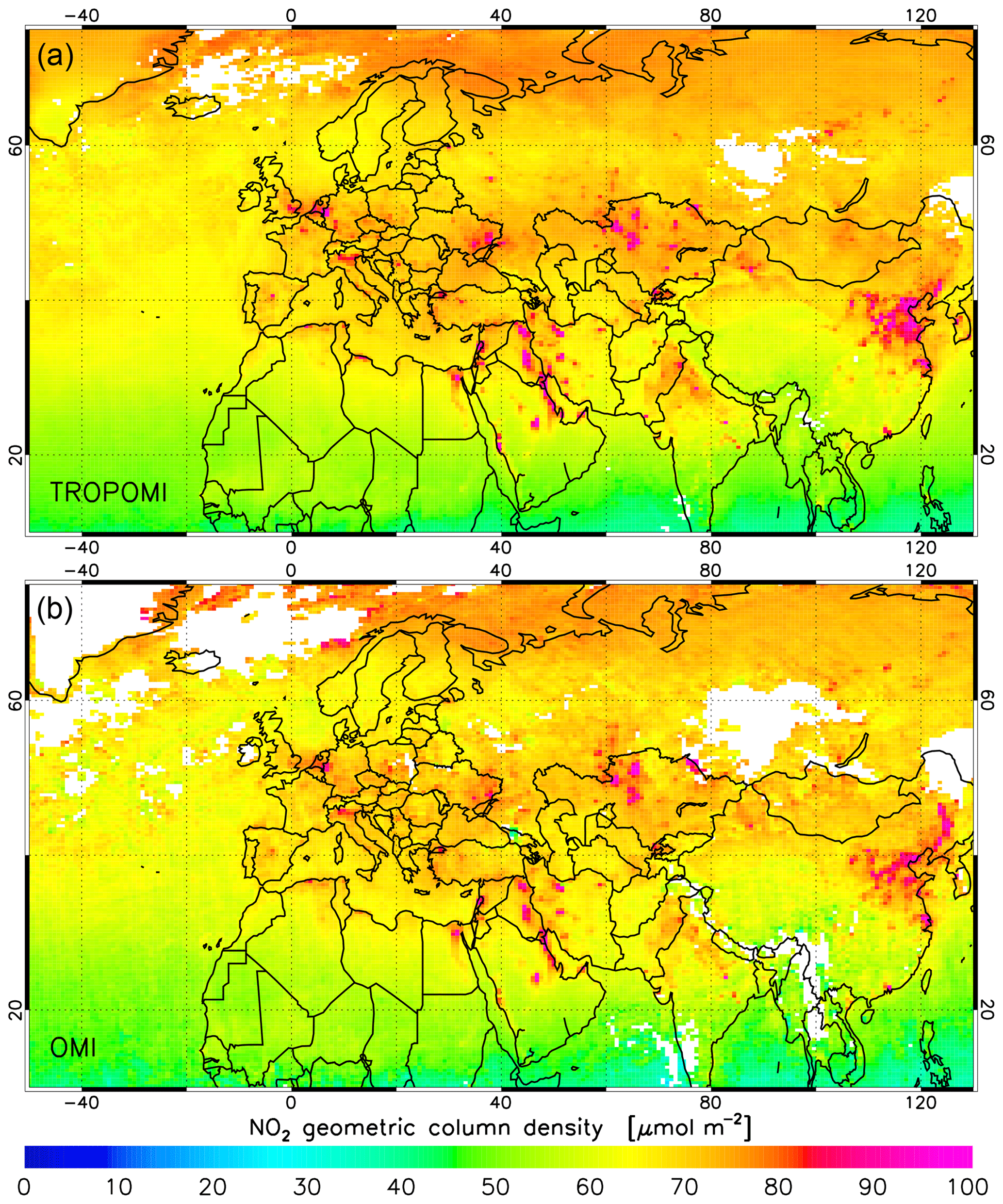
Figure 1NO2 geometric column density (GCD, defined in Sect. 4) from TROPOMI (a) and OMI–QA4ECV (b) averaged over 20–26 July 2019 on a common longitude × latitude grid of . Only clear-sky ground pixels (i.e. with cloud radiance fraction <0.5) are used. The OMI data are filtered for the row anomaly (Sect. 2.2.2).
OMI NO2 slant column data from QA4ECV (Boersma et al., 2018) can be used for comparisons (Sect. 4) because OMI and TROPOMI provide observations at almost the same local time. The example in Fig. 1 shows that both instruments capture the larger NO2 hotspots equally well but that OMI misses some smaller hotspots and that its measurements are noisier than TROPOMI's because the latter has a higher spatial resolution and a better signal-to-noise ratio.
TROPOMI level-2 data are reported in SI units, which for NO2 means in mol m−2. For convenience of the reader this paper uses the SI units and in most instances also provides numbers in the more commonly used unit of molec. cm−2; the conversion factor between the two is 6.02214×10¹⁹ mol−1.
2.1 TROPOMI aboard Sentinel-5 Precursor
2.1.1 TROPOMI instrument
TROPOMI (Veefkind et al., 2012) is a nadir-viewing spectrometer aboard ESA's S5P spacecraft, which was launched in October 2017. From an ascending sun-synchronous polar orbit, with an Equator crossing at about 13:30 local time, TROPOMI provides measurements in four channels (UV, visible, NIR and SWIR) of various trace gas concentrations, as well as cloud and aerosol properties. In the visible channel (400–496 nm), used for the NO2 retrieval, the spectral resolution and sampling are 0.54 and 0.20 nm, with a signal-to-noise ratio of around 1500. Radiance measurements are taken along the dayside of the Earth; once every 15 orbits a small part of the dayside orbit near the North Pole is used to measure the solar irradiance.
Individual ground pixels are 7.2 km (5.6 km as of 6 August 2019), with an integration time of 1.08 s (0.84 s), in the along-track and 3.6 km in the across-track direction at the middle of the swath. There are 450 ground pixels (rows) across-track and their size remains more or less constant towards the edges of the swath (the largest pixels are ∼14 km wide). The full swath width is about 2600 km and with that TROPOMI achieves global coverage each day, except for narrow strips between orbits of about 0.5∘ width at the Equator. Along-track there are 3245 or 3246 scanlines (4172 or 4173 after the along-track pixel size reduction) in regular radiance orbits, leading to about 1.46 (1.88) million ground pixels per orbit; for orbits with irradiance measurements there are about 10 % fewer scanlines. Approximately 15 % of the ground pixels are not processed due to the limit on the solar zenith angle () in the processing.
Over very bright radiance scenes, such as high clouds, the CCD detectors containing band 4 (visible; e.g. used for NO2 retrieval) and band 6 (NIR; e.g. used for cloud data retrieval) may show saturation effects (Ludewig et al., 2020), leading to lower-than-expected radiances for certain spectral (i.e. wavelength) pixels. In large saturation cases, charge blooming may occur: excess charge flows from saturated into neighbouring detector (ground) pixels in the row direction, resulting in higher than expected radiances for certain spectral pixels. Version 1.0.0 of the level-1b spectra contains flagging for saturation but not for blooming; version 2.0.0 will also have flagging for blooming (Ludewig et al., 2020).
2.1.2 TROPOMI observations used in this study
The TROPOMI NO2 data retrieval is described in the product Algorithm Theoretical Basis Document (ATBD; van Geffen et al., 2019); see also the Product User Manual (PUM; Eskes et al., 2019) and the Product ReadMe File (PRF; Eskes and Eichmann, 2019) for use of the data and the data product versions.
To investigate the stability and uncertainties of the TROPOMI NO2 SCDs, orbits over the Pacific Ocean, i.e. away from anthropogenic sources of NO2, are used: for each day the first available orbit with satellite (nadir-viewing) Equator crossings west of about −135 ∘. Such an orbit is missing on a few days and these days are thus skipped.
The TROPOMI data used in this study cover the period 30 April 2018 (which is the start of the operational (E2) phase) up to 31 January 2020. Offline (re)processed data of versions 1.2.x and 1.3.x are used; these versions do not differ in the SCD retrieval part of the processing and are based on level-1b version 1.0.0 spectra (Babić et al., 2017). Near real-time (NRT) data are not considered here; validation of both the offline and NRT data has shown that results of these processing chains do not differ significantly (Lambert et al., 2019).
2.2 OMI aboard EOS-Aura
2.2.1 OMI instrument
OMI (Levelt et al., 2006) is a nadir-viewing spectrometer aboard NASA's EOS-Aura spacecraft, which was launched in July 2004. From an ascending sun-synchronous polar orbit, with an Equator crossing at about 13:40 local time, OMI provides measurements in three channels (two UV and one visible) of various trace gas concentrations, as well as cloud and aerosol properties. In the visible channel (349–504 nm), used for the NO2 retrieval, the spectral resolution and sampling are 0.63 nm and 0.21 nm, with a signal-to-noise ratio of around 500. Radiance measurements are taken along the dayside of the Earth; once every 15 orbits a small part of the dayside orbit near the North Pole is used to measure the solar irradiance.
Individual ground pixels are 13 km, with an integration time of 2 s, in the along-track and 24 km in the across-track direction at the middle of the swath. There are 60 ground pixels (rows) across-track and their size increases towards the edges of the swath to ∼150 km. The full swath width is about 2600 km, and with that OMI achieves global coverage each day. Along-track there are 1643 or 1644 scanlines in regular radiance orbits, leading to just under 100 000 ground pixels per orbit; for orbits with irradiance measurements there are about 10 % fewer scanlines.
2.2.2 OMI observations used in this study
Comparisons of the magnitude of the NO2 SCDs of TROPOMI and OMI are done using OMI orbits from 2018 to 2019 as processed within the framework of the QA4ECV project (Boersma et al., 2018). Since June 2007 a part of the OMI detector has suffered from a so-called row anomaly, which appears as a signal suppression in the level-1b radiance data at all wavelengths (Schenkeveld et al., 2017), leading, e.g., to large uncertainties in the NO2 SCDs in the affected rows 22–53 (0-based). Comparisons of the NO2 SCD uncertainties (Sect. 4.1) are also made with OMI Pacific Ocean orbits from 2005–2006, the first year after launch, before the row anomaly occurred. Note that the OMI degradation over the past 15 years is small: the SCD statistical uncertainties and SCD error estimates have increased by about 1 % and 2 % per year, respectively (Zara et al., 2018).
TROPOMI and OMI measure at about the same local time (the Equator crossing local time differs by about 10 min) but since TROPOMI travels at about 830 km and OMI at about 715 km altitude, TROPOMI orbits take a little longer than OMI's: when TROPOMI has completed one orbit, OMI has covered ∼1.03 orbits. This means that if a given two orbits exactly overlap, then 19 orbits later TROPOMI's Equator crossing longitude lies in between the Equator crossing longitudes of two OMI orbits, i.e. a longitudinal mismatch of about 12.5∘. The difference in orbit overlap plays a role when comparing results from individual orbits (as done in Sect. 4.1) but is not relevant in the case of gridded averaged data being used (as done in Fig. 1 and Sect. 4.4).
2.3 Latitudinal range for uncertainty studies
To investigate the stability and uncertainties of the NO2 SCD retrieval the “tropical latitude” (TL hereafter) range is defined as all scanlines that have their sub-satellite latitude point – corresponding approximately to the nadir-viewing detector rows – within a 30∘ range that moves along with the seasons, in an attempt to filter out seasonality in the NO2 columns: on 1 January the TL range covers [−30 ∘ , 0 ∘] for the sub-satellite latitude points, while half a year later it covers [0 , +30 ∘]. The TL range is also used for the across-track “de-striping” of the SCDs discussed in Sect. 4.3. For TROPOMI (OMI) data the TL range contains about 475 (250) scanlines; after the along-track pixel size reduction in TROPOMI there are about 610 scanlines in the TL range.
van Geffen et al. (2015)van Geffen et al. (2019)Danckaert et al. (2017)Boersma et al. (2018)Rodgers (2000)Press et al. (1997, ch. 15)Dobber et al. (2008)Vandaele et al. (1998)Serdyuchenko et al. (2014)Thalman and Volkamer (2013)Rothman et al. (2013)Pope and Fry (1997)Chance and Spurr (1997)Table 1Specifics for the NO2 slant column retrieval of TROPOMI and OMI–QA4ECV. The reference spectra (second group of entries) have all been convolved with the row-dependent instrument spectral response function (ISRF or slit function). Last access dates for all websites mentioned in the table is 17 March 2020.
a Specifics of the OMI–OMNO2A retrieval are mentioned in Sect. 3.4. b Offline (re)processing uses E0 measured nearest in time to I, except for the period mid-October 2018 to mid-March 2019, when the most recent E0 with regard to I was used due to an issue with the processor; the version-2 reprocessing will use the nearest E0 for all orbits.
Though this paper discusses the method and results of the TROPOMI NO2 slant column retrieval (Sect. 3.2), it is important to also discuss the retrieval method used for OMI data within the QA4ECV (Sect. 3.3) and OMNO2A (Sect. 3.4) approaches because differences in results (Sect. 4) turn out to be mainly related to retrieval method details.
3.1 DOAS technique
The NO2 SCD retrieval is performed using a DOAS technique (Platt, 1994; Platt and Stutz, 2008), which provides the amount of NO2 along the effective light path, from sun through atmosphere to satellite. This technique attempts to model the reflectance spectrum Rmeas(λ) observed by the satellite instrument:
with I(λ) the radiance at the top of the atmosphere, E0(λ) the extraterrestrial solar irradiance measured by the same instrument and μ0=cos (θ0) the cosine of the solar zenith angle; given that the processing is limited to ground pixels measured at , the division by μ0 in Eq. (1) will not cause problems. Note that both I and E0 also depend on viewing geometry, but those arguments are left out for brevity.
The modelled reflectance, Rmod(λ), is determined from reference spectra of a number of species known to absorb in the wavelength window used for the SCD retrieval, as well as a correction for scattering and absorption by rotational Raman scattering (RRS), the so-called “Ring effect” (see Grainger and Ring, 1962; Chance and Spurr, 1997), while a polynomial () is used to account for spectrally smooth structures resulting from molecular (single and multiple) scattering and absorption, aerosol scattering and absorption, and surface albedo effects.
The precise formulation of Rmod(λ) and the method used to minimise the difference between the modelled and measured reflectance differs slightly between the TROPOMI and OMI retrievals. Details of these DOAS approaches are listed in Table 1. (The difference in the degree of the DOAS polynomial is not relevant: np=4 and np=5 give practically the same results; for TROPOMI np=5 is chosen following the traditional setting in the OMNO2A processing (cf. Sect. 3.4) of OMI data.)
3.2 TROPOMI intensity fit retrieval
In the TROPOMI NO2 processor (van Geffen et al., 2019) Rmod(λ) is formulated in an intensity fit (IF hereafter) approach:
with σk(λ) the absolute cross section and Ns, k the slant column amount of molecule taken into account in the fit: NO2, ozone, water vapour, liquid water and the O2−O2 collision complex. The physical model accounts for inelastic Raman scattering of incoming sunlight by N2 and O2 molecules that leads to the filling-in of the Fraunhofer lines in the radiance spectrum, i.e. the Ring effect. In Eq. (2), Cring is the Ring fit coefficient and Iring(λ)∕E0(λ) the sun-normalised synthetic Ring spectrum, with E0(λ) is the measured irradiance. The term between parentheses in Eq. (2) describes both the contribution of the direct differential absorption (i.e. the 1), and the modification of these differential structures by inelastic scattering (the term) to the reflectance spectrum.
The IF minimises the chi-squared merit function:
with nλ the number of wavelengths (spectral pixels) in the fit window (405–465 nm) and ΔRmeas(λi) the uncertainty in the measured reflectance, which depends on the precision of the radiance and irradiance measurements as given in the level-1b product, i.e. on the signal-to-noise ratio (SNR) of the measurements. Radiance spectral pixels flagged in the level-1b data as bad or as suffering from saturation (Sect. 2.1.1) are filtered out before any further processing step.
In the final data product ground pixels are flagged when the slant column retrieval uncertainty ΔNs>33 µmol m−2 (2×10¹⁵ molec. cm−2). SCD error values this large occur rarely: usually <0.1 % of the pixels per orbit with original ground pixel sizes; for the smaller-size pixel orbits there are about 50 % more pixels with high SCD error values (based on one test day of data), taking into account that the SCD error itself increases with reduced pixel size. Note, however, that the ground pixel size reduction leads to about 28 % more ground pixels per orbit and thus a significant increase in the number of successfully retrieved ground pixels.
The magnitude of χ2 is a measure of how good the fit is. Another measure of the goodness of the fit is the so-called root-mean-square (rms) error:
where the difference is usually referred to as the residual of the fit.
In the TROPOMI processor χ2 is minimised using an optimal estimation (OE; based on Rodgers, 2000) routine, with suitable a priori values of the fit parameters and a priori errors set very large, so as not to limit the solution of the fit (for example, the NO2 SCD a priori error is set at mol m molec. cm−2), while for numerical stability reasons a pre-whitening of the data is performed. Estimated slant column and fitting coefficient uncertainties are obtained from the diagonal of the covariance matrix of the standard errors, while the off-diagonal elements represent the correlation between the fit parameters.1 The SCD error estimates are scaled with the square root of the normalised χ2, where χ2 is normalised by (nλ−D), with D the degrees of freedom of the fit, which is almost equal to the number of fit parameters: , with the SCD error reported by the OE routine. The NO2 output data product provides and rms error.
3.2.1 TROPOMI wavelength calibration
Before forming the reflectance of Eq. (1) both I(λ) and E0(λ) are calibrated, after which the calibrated E0(λcal) is interpolated, using information from a high-resolution reference spectrum (Eref; see Table 1), to the calibrated I(λcal), which serves as the common grid for the reflectance. In the TROPOMI processor these steps are performed prior to the DOAS fit (van Geffen et al., 2019).
A wavelength calibration essentially replaces the nominal wavelength λnom that comes along with the level-1b spectra (Ludewig et al., 2020) by a calibrated version:
where ws represents a wavelength shift and wq a wavelength stretch (wq>0) or squeeze (wq<0), with wq defined with regard to the central wavelength of the fit window λ0. Each radiance ground pixel and each irradiance row has its own wavelength grid and calibration results. In the TROPOMI processor fitting wq is turned off; see below for a short discussion of this.
The wavelength calibration is performed over the full NO2 fit window (405–465 nm), using a high-resolution solar reference spectrum (Eref, pre-convolved with the TROPOMI instrument spectral response function (ISRF); see Table 1) and the OE routine also in use for solving the DOAS equation. For the I(λ) calibration a second-order polynomial as well as a term representing the Ring effect are included: the model function used for the radiance wavelength calibration is a modified version of Eq. (2); including the Ring effect allows for a wavelength calibration to be performed across the full fit window. For the E0(λ) calibration the Ring term is obviously excluded. The a priori error of the wavelength shift is set to 0.07 nm, one-third of the spectral sampling in the NO2 wavelength range, so as to ensure that ws will not exceed the spectral sampling distance.
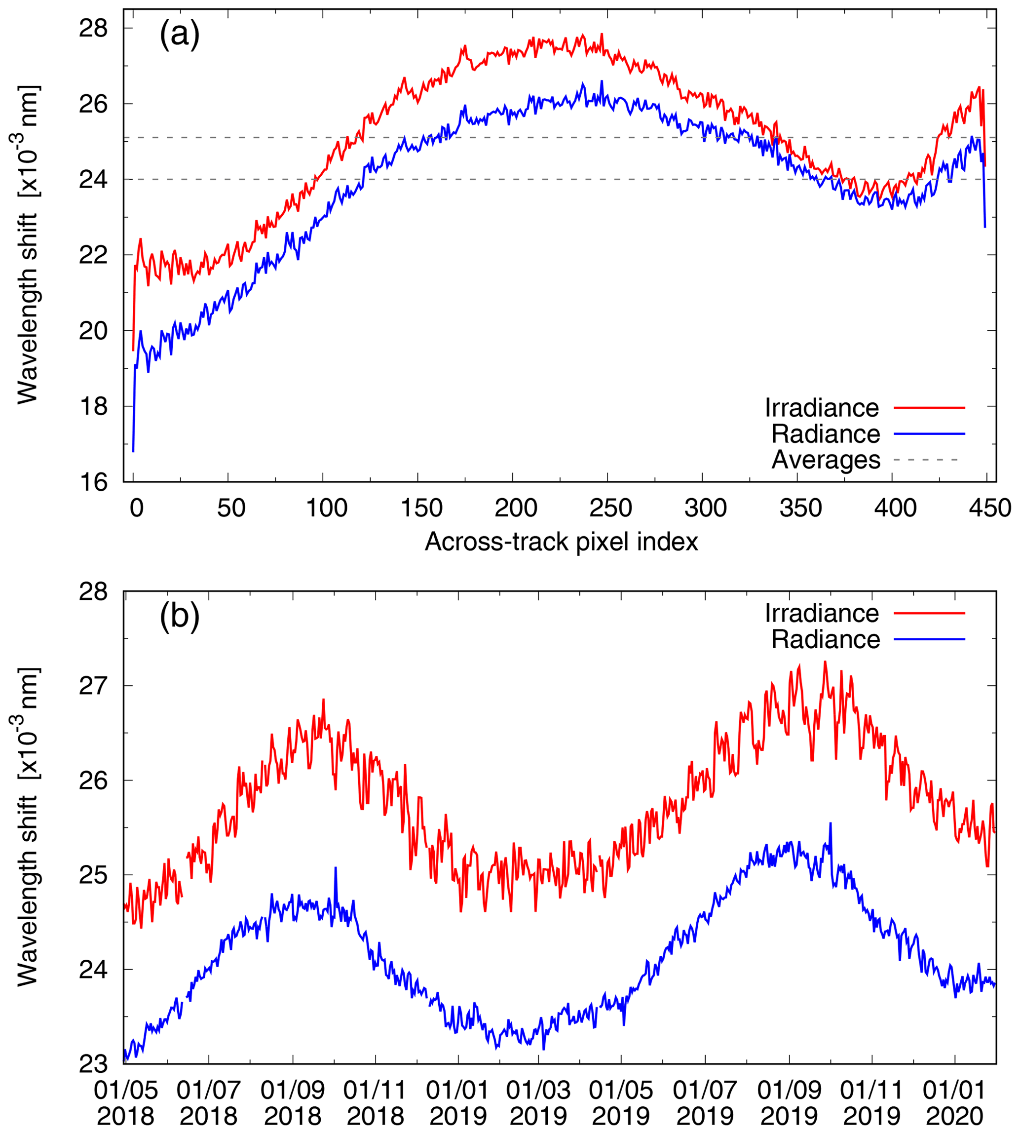
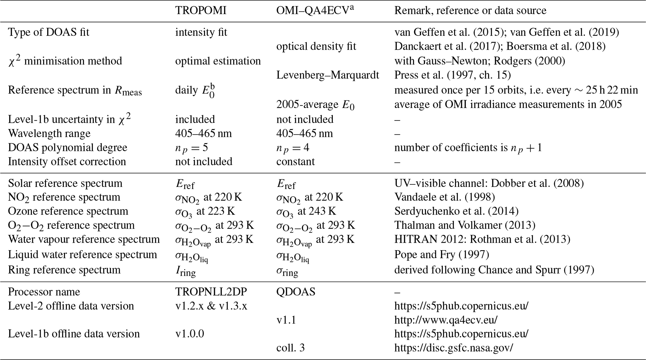
Figure 2Wavelength calibration shifts ws for the NO2 fit window (405–465 nm) of the TROPOMI irradiance (red) and radiance (blue), where the latter is an average over the tropical latitude (TL) range. (a) Shifts for 1 July 2018 (radiance orbit 03711, with irradiance from orbit 03718) as a function of the across-track ground pixel index; the dashed horizontal lines are the across-track averages, with the exception of the outer rows. (b) Time evolution of the across-track average shifts.
Figure 2a shows the wavelength shifts ws for an orbit on 1 July 2018 of the irradiance (red) and radiance (blue) as a function of across-track ground pixel (row), where the radiance shift of each row is an along-track average over the TL range defined in Sect. 2.3. When taking a different latitude range the across-track shape of the radiance wavelength shift shown in Fig. 2a does not noticeably change, while the absolute value of the average shifts increases by about 5 % going south to north – it is not known what causes this small increase, but it is well within instrument specifications. Due to only partial instrument slit illumination at the outer two rows, 0 and 449, ws shows markedly different values for these rows. To avoid these peaks from overshadowing the effects discussed below, the outer two rows are skipped from the following analysis.
The broad across-track shape and the average value of ws visible in Fig. 2a are not important, as they result from the choice of the nominal grid of the level-1b data. The change in time of the average and of the row-to-row variation in ws, however, give an idea of the stability of the level-1b data and hence of the instrument. Figure 2b shows the temporal change in . There seems to be a small long-term oscillation in this, with an amplitude of about 0.0016 and 0.0020 nm for radiance and irradiance, respectively, which looks likely to be a seasonal effect. A similar seasonal variation of similar amplitude is seen in the wavelength calibration data of OMI's visible channel (Schenkeveld et al., 2017, Fig. 34). Both for TROPOMI and OMI this amplitude does not exceed scatter levels and is thus well within instrument requirements.
For a given field of view (ground pixel), the dominant term in the overall magnitude of the radiance is the inhomogeneous illumination of the instrument slit as a result of the presence of clouds. Variation in the presence of clouds may therefore show up as differences in the ws of ground pixels (e.g. along a row) and from day to day. The magnitude of the day-to-day variation in the average is much smaller than the long-term oscillation visible in Fig. 2b. The row-to-row variation in the shift, visible in Fig. 2a, is small and the evolution of that across-track variation shows a slow increase over time (not shown), probably related to degradation of the instrument (Erwin Loots, personal communication, 2019).
With the forthcoming update of the level-1b data to v2.0.0 the nominal UV–visible wavelength grids of both irradiance and radiance are adjusted by 0.027 nm, for all rows and all days (Ludewig et al., 2020). As a result of this the average will be reduced by that amount, but the across-track and in-time variations will remain the same. Level-1b v2.0.0 will contain an improved degradation correction (Rozemeijer and Kleipool, 2019; Ludewig et al., 2020), probably reducing the slow increase over time of the across-track variation mentioned above. All in all, the wavelength calibration results show that TROPOMI is a rather stable instrument, but further monitoring of the wavelength shifts seems worthwhile.
Turning on the stretch fit parameter in the radiance calibration for orbit 03711 leads to a small stretch of 0.2–, depending on latitude, with an associated error estimate of 3– (averaging over 30∘ latitude ranges with varying central latitudes): the stretch found is smaller than its error for most latitudes. At the same time the radiance wavelength shift, the NO2 SCD and SCD error, and the rms error of the DOAS fit change on average by less than 1 %, with a standard deviation comparable to that change or larger. In other words: including the stretch fit parameter in the radiance calibration does not significantly alter the retrieval results, and hence the wq fit parameter will remain turned off.
3.3 OMI–QA4ECV optical density fit retrieval
The OMI data are processed in the QA4ECV framework with the QDOAS software (Danckaert et al., 2017), wherein Rmod(λ) is formulated in an optical density fit (ODF hereafter) approach:
with σring(λ) the differential (pseudo-absorption) reference spectrum of the Ring effect and Cring its fitting coefficient, where σring(λ) equals Iring(λ)∕Eref(λ) minus a second-order polynomial, with Eref a (constant) solar reference spectrum (which is different from the measured solar spectrum E0(λ) used in Eq. 2). Note that except for the way the Ring effect is treated, the IF and ODF modelled reflectances are the same to first order; see Appendix A for a discussion of this difference.
The ODF minimises the merit function (cf. Eq. 3):
without weighting with the level-1b uncertainty estimate ΔRmeas, though QDOAS has the option to include the weighting. To minimise , QDOAS uses a Levenberg–Marquardt non-linear least-squares fitting procedure (Press et al., 1997), which also provides an estimate of the uncertainties in the fit parameters.
In the ODF formulation the rms error is defined as
which is different from the Rrms of the intensity fit as given in Eq. (4); see Appendix B for a relationship between the two.
Like many other DOAS applications, the OMI–QA4ECV processing includes a correction for an intensity offset in the radiance:
with Poff(λ) a low-order polynomial (in OMI–QA4ECV a constant) and Soff a suitable scaling factor (QDOAS computes this dynamically from an average of the measured solar spectrum E0(λ) in the DOAS fit window). Sect. 5.1 discusses the possible origin and implication of this correction term.
QDOAS also has the option to be run in intensity fit mode, in which case the modelled reflectance includes the Ring effect as a pseudo-absorber like it does in the optical density fit mode Eq. (6) rather than as the non-linear term like in Eq. (2).
3.3.1 OMI–QA4ECV wavelength calibration
In QDOAS (Danckaert et al., 2017) the wavelength calibration of E0(λ) is performed prior to the DOAS fit, based on a high-resolution solar reference spectrum (Eref; see Table 1). The calibration of I(λ) is part of the DOAS fit: the shift, ws, and stretch, wq, are fitted along with the SCDs, with the calibrated E0(λcal) wavelength grid as the common grid for the reflectance. For OMI–QA4ECV both a shift and stretch are fitted (cf. Eq. 5) with the stretch negligibly small. When processing TROPOMI data with QDOAS, only shifts are fitted, as is the case for the regular TROPOMI processing.
Processing the TROPOMI orbit for which the wavelength shifts are shown in Fig. 2a with QDOAS leads to almost identical wavelength shifts: the irradiance and TL average radiance shifts differ by nm and nm, respectively (the TROPOMI spectral sampling is 0.20 nm; Sect. 2.1.1). Consequently, the difference in radiance wavelength calibration between TROPOMI and QDOAS will not affect comparisons of the retrieval results noticeably.
3.4 OMI–OMNO2A intensity fit retrieval
The official OMI NO2 SCD data processing, running at NASA, is called OMNO2A. OMNO2A v1.2.x delivers the SCD data for the DOMINO v2 NO2 vertical column density (VCD) processing (results of which are released via http://www.temis.nl/airpollution/no2.html, last access: 17 March 2020). A number of improvements intended for OMNO2A v2.0, which have not yet been implemented, were investigated by van Geffen et al. (2015), but the SCD retrieval of OMNO2A v2.0 can be run locally at the Royal Netherlands Meteorological Institute (KNMI) for testing and comparisons. The OMNO2A processor does not include an intensity offset correction term.
OMNO2A v2.0 uses the intensity fit approach with the modelled reflectance formulated in the same manner as TROPOMI, viz. Eq. (2) and the settings listed for TROPOMI in Table 1, with the exception that χ2 is minimised using a Levenberg–Marquardt (LM) solver and wavelength calibration is performed over part of the NO2 fit window (409–428 nm), the 2005 average irradiance spectrum as reference and an older ozone reference spectrum (van Geffen et al., 2015). Tests have shown that the LM and OE solvers essentially give the same fit results when used with the same settings. Furthermore, KNMI has a local tool to convert the OMI level-1b data into the TROPOMI level-1b format, enabling direct comparisons between the two processors.
Figure 3NO2 geometric column density (GCD, defined in Sect. 4; a, b, c) and slant column density (SCD) error estimate from the DOAS fit (d, e, f) averaged over the TL range as function of the across-track viewing zenith angle (θ) of Pacific Ocean orbits of TROPOMI and OMI on 1 July 2018 and of OMI on 1 July 2005. (a, d) Regular TROPOMI processing of TROPOMI compared with OMI–QA4ECV processing. (b, e) Regular TROPOMI processing of TROPOMI compared with QDOAS processing with TROPOMI settings and with QA4ECV settings. (c, f) Regular TROPOMI processing of OMI compared with OMI–QA4ECV and OMNO2A (v2) results.
This section discusses the NO2 SCD retrieval results of selected TROPOMI orbits in comparison with OMI orbits and additional retrieval results using QDOAS (Danckaert et al. (2017); version r1771, dated 20 March 2018, is used here).
The SCD depends strongly on the along-track and across-track variation in solar zenith angle (θ0) and viewing zenith angle (θ). To make evaluations and comparisons easier, the SCD is divided by the geometric AMF, defined as , which is a simple but realistic approximation for the air-mass factor for stratospheric NO2. The resulting NO2 total column may be called the geometric column density (GCD), to distinguish it from the total, tropospheric and stratospheric VCDs, which are determined using AMFs based on NO2 profile information coming from the CTM/DA model (see Sect. 1).
4.1 GCD and SCD error comparison for one orbit
Figure 3 provides comparisons of the GCD (left column) and SCD error estimate from the DOAS fit (right column), averaged over the TL range for the Pacific Ocean orbits of TROPOMI and OMI on 1 July 2018. In view of the OMI row anomaly, the corresponding OMI orbit of 1 July 2005 is shown as well, noting that the NO2 concentrations in 2005 are likely to be different from those in 2018.
The TROPOMI orbit used here is representative of all Pacific Ocean orbits in across-track shape and variability, as is shown in subsequent sections by the stability of stripe amplitude (Sect. 4.3) and slant column uncertainties (Sect. 4.6).
4.1.1 Geometric column density
In Fig. 3a the GCD results of the regular TROPOMI processing are compared with the OMI–QA4ECV processing. The TROPOMI and OMI GCD of 1 July 2018 compare well in magnitude, in as far as such a comparison is possible in view of the large row-to-row variation in the OMI data and the row anomaly: averaged over the viewing zenith angle range TROPOMI's GCD is about 3 % higher than OMI's. Near the western (left) edge of the swath, TROPOMI seems to report lower NO2 values than OMI, which might be related to the fact that nadir of the OMI orbit lies 9∘ east of TROPOMI nadir. The OMI GCD of 1 July 2005 clearly shows less row-to-row variation than the OMI 2018 data but more than the TROPOMI data (cf. Sect. 4.3).
In Fig. 3b the regular TROPOMI results are compared with a processing of the TROPOMI level-1b data with QDOAS, using settings as close as possible to those of the TROPOMI processor and settings used for QA4ECV (viz. Table 1). When using TROPOMI settings the QDOAS results match those of the regular TROPOMI processing very closely: averaged over the central 150 (of the 450) detector rows the difference is about 0.2 %. The QDOAS QA4ECV settings are different from the TROPOMI settings at three points (type of DOAS fit, use of level-1b uncertainly in χ2 minimisation and intensity offset correction), as a result of which the GCDs (and thus the SCDs) are lower by about 6.1 % for this orbit. Sect. 4.2 discusses the effect of the QDOAS settings somewhat further.
In Fig. 3c the OMI results of the regular QA4ECV processing are compared with a processing of the OMI level-1b data with the OMNO2A and TROPOMI SCD processors for the OMI orbit of 2005 in Fig. 3a, in order to investigate the impact of retrieval method details. Differences in the results of the OMNO2A and TROPOMI processor are likely mainly due to differences in the wavelength calibration: TROPOMI's radiance wavelength calibration includes a correction for the Ring effect, which allows the use of a larger calibration window (in this case the NO2 fit window; viz. Sect. 3.2.1), while OMNO2A's calibration window is necessarily limited (viz. Sect. 3.4).
As with the TROPOMI data in Fig. 3b, the QA4ECV settings clearly give the lowest GCD results: averaged over the central 20 (of the 60) detector rows, the QA4ECV GCD is lower than the OMNO2A processor GCD by about 3.7 % and lower than the TROPOMI processor GCD by about 7.0 %. Note that the across-track striping in the OMI results differs markedly between the different processor results, which is related to a combination of processor differences and the response to instrumental issues (OMI striping data quoted in Sect. 4.3 is taken from OMI–QA4ECV).
Table 2NO2 geometric column density (GCD), slant column density (SCD) error and rms error from the DOAS fit averaged over the TL range and the central 150 detector rows of TROPOMI Pacific orbit 03711 of 1 July 2018 retrieved with QDOAS using different settings. For comparison, the regular v1.2.2 TROPOMI results (used in this study) and a local reprocessing using the forthcoming v2.1.0 are also listed. Given the difference in rms error definitions, their values from QDOAS and TROPOMI retrievals cannot be compared directly (Sect. 3.3).
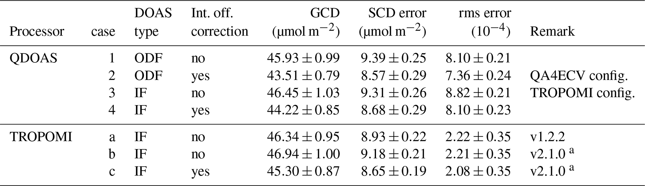
a With respect to v1.2.2, v2.1.0 entails two small bug fixes and spike removal (Sect. 4.1.3); all QDOAS runs include spike removal.
4.1.2 Slant column density error
In the case of TROPOMI, on-board across-track binning of measurements takes place: for the outer 22 (20) rows at the left (right) edge of the swath, the binning factor is 1, while for the other rows 2 detector pixels are combined, in order to keep the across-track ground pixel width more or less constant. As a result of this, the outer rows have a larger spectral uncertainty, which is reflected in a larger SCD error. The increased SCD error visible in the TROPOMI data of Fig. 3d, e around is related to the presence of saturation effects above bright clouds along this particular orbit.
Figure 3d–f shows that the SCD error estimate for TROPOMI data is considerably lower than the estimates for OMI–QA4ECV data. Given that the TROPOMI and OMI retrievals are performed with different methods, a direct comparison between SCD error is only tentative; an independent method to compare SCD uncertainties is discussed in Sect. 4.6. Averaged over , i.e. away from the row anomaly, TROPOMI's SCD error is about 40 % (30 %) lower than OMI's 2018 (2005) data.
The reason why the OMI SCD error in 2018 is higher than in 2005 (Fig. 3d) is, at least partly, related to the fact that in the OMI processing the 1-year average irradiance of 2005 is used for all retrievals, and the larger the time difference between radiance and irradiance measurements, the larger the error on the reflectance and thus on the SCD error is (cf. Sect. 4.5). This issue has been discussed in detail by Zara et al. (2018).
Figure 3e shows that the TROPOMI SCD error estimate compares reasonably well with the estimate provided by QDOAS, despite the differences in retrieval methods: averaged over the central 150 detector rows the difference is about +4.2 % with TROPOMI settings and about −2.0 % with QA4ECV settings (see also Sect. 4.2). Figure 3f shows that in the case of OMI data the SCD error is lowest for the regular QA4ECV retrieval: the TROPOMI processor reports a 10.2 % higher and the OMNO2A processor a 15.4 % higher SCD error.
4.1.3 Impact of NO2 processor updates to v2.1.0
An update of the level-2 NO2 SCD data to version 2.1.0 (planned for late 2020;2 van Geffen et al., 2020) entails two small bug fixes in the wavelength assignment and better treatment of saturated radiance spectral pixels and of outliers in the residual (Appendix C). These improvements have a small impact on the absolute value of the NO2 SCD, SCD error and rms error of the fit: on average +0.5 %, +2.5 % and −1 %, respectively, based on a set of test orbits (see also Table 2). These changes are not expected to alter the averages and temporal stability presented in this paper significantly.
TROPOMI level-1b version 1.0.0 spectra suffer from a small degradation (Rozemeijer and Kleipool, 2019) of 1 %–2 %, notably in the irradiance. The update of the level-1b spectra to version 2.0.0 (planned for late 2020) will include a correction for the degradation, as well as some calibration corrections and improved flagging of saturation and blooming effects in some spectral pixels (Ludewig et al., 2020). This update will have a small impact on the absolute value of the NO2 SCD, SCD error and rms error of the fit: on average +2 %, −1 % and −6 %, respectively, based on the evaluation of 12 test orbits. A reprocessing of all E2 phase data using v2.0.0 level-1b spectra and NO2 v2.1.0 will probably take place sometime in 2020–2021.
4.2 TROPOMI NO2 SCD: different QDOAS options
As mentioned in the previous section (and visible in Fig. 3), the retrieval results depend on the details of the DOAS NO2 SCD retrieval: the type of the DOAS fit (IF or ODF) and the retrieval settings used (in particular whether the intensity offset correction is included or not).
Table 2 presents the GCD, SCD error and rms error of the DOAS fit for four combinations of QDOAS settings when processing TROPOMI orbit 03711, with other configuration settings as much as possible matching those of the TROPOMI processor (if included, the intensity offset correction polynomial Poff(λ) is a constant), as well as the results from the TROPOMI NO2 processor. Conclusions from these results are as follows:
-
Turning on the intensity offset correction in QDOAS has quite a large impact on the results: the GCD goes down by ∼5 %, while the SCD error goes down by ∼8%.
-
That turning on the intensity offset correction in QDOAS leads to a lower rms error is logical, since an extra fit parameter is introduced; it cannot be determined which part of the reduction in the rms error (by ∼9 %) is due to this extra fit parameter and which part is due to a physically better fit.
-
In IF mode QDOAS retrieves slightly larger GCDs (∼1 %) and slightly lower SCD errors (∼1 %), showing that the precise fit method itself does not affect the fit results much.
-
The rms error calculation of the TROPOMI IF mode and the QDOAS ODF mode, given in Eqs. (4) and (8), respectively, lead to different results; a relation between these two is given in Appendix B.
-
Given that the rms error in the QDOAS IF mode is ∼9 % higher than in the QDOAS ODF mode the rms definitions of these two QDOAS modes may be slightly different for the two modes and the definition of the QDOAS IF mode is different from the TROPOMI IF mode.
As a reference, Table 2 also includes the results of the regular TROPOMI retrieval of the currently officially available processor version v1.2.2, as well as the results from a local reprocessing with the forthcoming v2.1.0 processor (Sect. 4.1.3). That processor has an experimental option to also include an intensity offset correction, implemented in the form of an extra term on the right-hand side of Eq. (2):
with Poff(λ) a low-order polynomial and Soff a suitable scaling factor with the same unit as E0(λ). Table 2 shows that including a constant Poff in the TROPOMI retrieval has a similar effect as in the case of QDOAS: the GCD and the SCD error decrease by a few percent.
Another small difference in the retrieval methods is that the TROPOMI NO2 processor uses the level-1b uncertainty in χ2 minimisation (cf. Eq. 3) whereas OMI–QA4ECV does not (cf. Eq. 7). QDOAS has the option to turn the χ2 weighting on in its ODF mode, the impact of which on the fit results (not shown) is minimal for the GCD and rms, while the SCD error seems to be unrealistically much reduced, indicating that perhaps the error propagation in the ODF mode is not done entirely correctly.
All in all, the retrieval method itself (IF or ODF) does not seem to have a significant impact, while the intensity offset correction has quite a large impact on the GCD (and thus on the SCD) values. The intensity offset term is further discussed in Sect. 5.1.
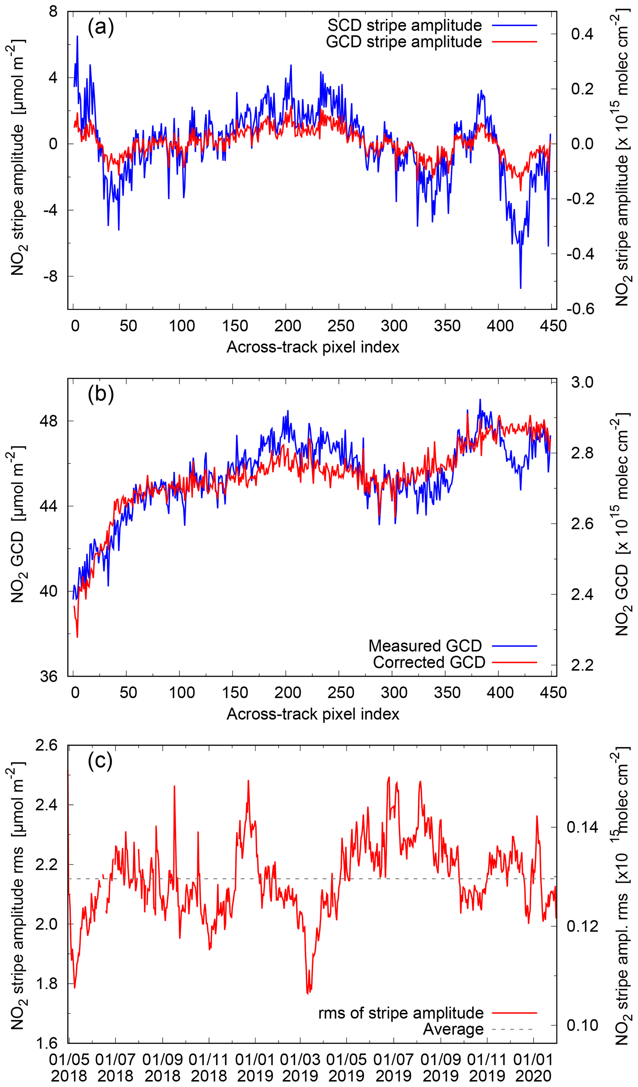
Figure 4Evaluation of the NO2 SCD stripe amplitude. (a) SCD stripe amplitude (blue) and , i.e. the GCD stripe amplitude (red), for orbit 03711 of 1 July 2018. (b) The measured (blue) and corrected (red) GCD for the same orbit, averaged over the TL range. (c) Time evolution of the rms of the SCD stripe amplitude.
4.3 De-striping: correcting across-track features
Since the beginning of the OMI mission, non-physical across-track variations in the NO2 SCDs have been observed, which shows up as small row-to-row jumps or “stripes” (Boersma et al., 2011; Veihelmann and Kleipool, 2006). Given that the geophysical variation in NO2 in the across-track direction (east–west) is smooth rather than stripe-like over non-contaminated areas (Boersma et al., 2007), a procedure to “de-stripe” the SCDs is implemented in the CTM/DA processing system used for DOMINO and QA4ECV. Even though in TROPOMI the row-to-row variation is much smaller than in OMI (cf. Fig. 3a), as of v1.2.0 it was decided to turn on de-striping to remove small but systematic across-track features and improve the data product quality.
The operational TROPOMI de-striping is determined from the TL range of orbits over the Pacific Ocean, and a slant column stripe amplitude is determined for each viewing angle. The SCD stripe amplitude () is defined as the difference between the measured total SCD (Ns) and the total SCD () derived from the CTM/DA profiles using the averaging kernel and air-mass factor from the retrieval. In order to retain only features which are slowly varying over time, and in order to reduce the sensitivity to features observed during a single overpass, the SCD stripe amplitudes are averaged over a time period of 7 d, or about seven Pacific orbits, before subtracting them from the SCDs. The NO2 data product file contains Ns and , so that a user of the slant column data can or must apply the stripe correction.
As an example, Fig. 4a shows for the Pacific Ocean orbit of 1 July 2018 (blue) and (red) for the stripe amplitude in GCD space. For the same orbit Fig. 4b shows the GCD (blue) averaged over the TL range and the corrected GCD, i.e. (red). The across-track structure and the magnitude of the vary in time, but the overall behaviour is fairly constant.
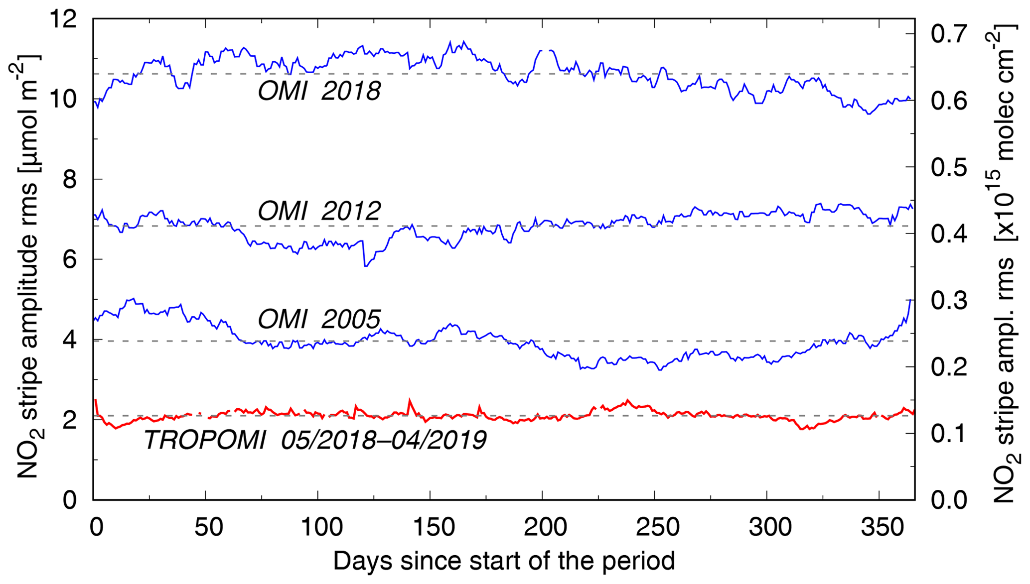
Figure 5Comparison of the time evolution of the rms of the NO2 SCD stripe amplitude over the first year of TROPOMI data (red; cf. Fig. 4c) and over selected OMI–QA4ECV years (blue); the main increases in the OMI rms occur during 2006, 2010–2011 and 2014–2015. Dashed lines indicate averages over the year periods.
A measure of the stability of the SCD stripe amplitude is the rms of the across-track stripe amplitude, i.e. of the blue line in Fig. 4a: , with summation over rows . Fig. 4c shows this rms as function of time: there is quite some variation, but on average the rms seems constant at 2.15±0.13 µmol m−2 ( molec. cm−2); nothing special is seen at 6 August 2019, when the pixel size changes. Further monitoring will have to show whether the stripe amplitude remains stable.
Figure 5 shows the same quantity for the first year of TROPOMI data (average: 2.10 µmol m−2) and for selected years of OMI–QA4ECV data: 2005 (3.96 µmol m−2 or 1.9 times the TROPOMI average), 2012 (6.83 µmol m−2 or 3.3 times) and 2018 (10.63 µmol m−2 or 5.1 times). The increase in the stripe amplitude of OMI NO2 data is not uniform over time and is also present in the case daily solar irradiance spectra being used for the retrieval (Sergey Marchenko, personal communication, 2019); hence the increase is not (or at least not solely) caused by the use of a fixed irradiance in the OMI–QA4ECV data processing (viz. Table 1),
4.4 Quantitative TROPOMI-OMI GCD comparison
The comparison of TROPOMI and OMI–QA4ECV Pacific Ocean orbits of 1 July 2018 in Fig. 3a is merely qualitative because (a) of the row anomaly in the OMI data, (b) of the stripiness of the OMI data and (c) the orbits do not exactly overlap. For a more quantitative comparison, TROPOMI and OMI data are gridded to a common longitude–latitude grid of , after applying the respective de-striping of the SCDs described in the previous subsection on both datasets.
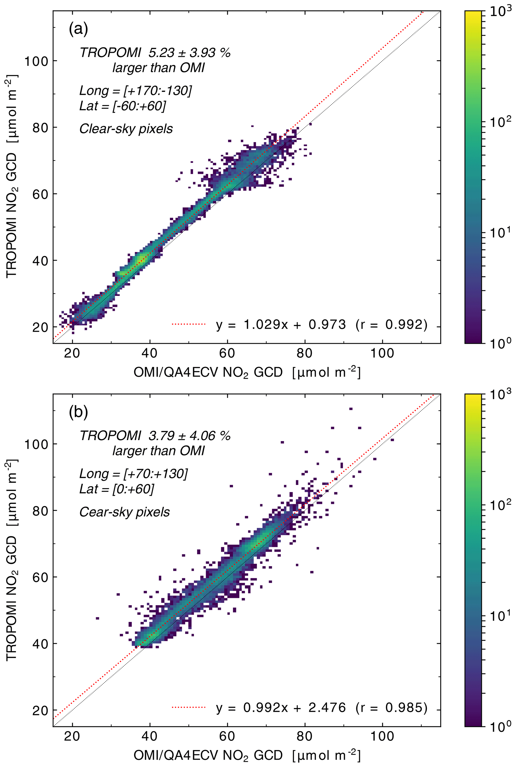
Figure 6Comparison of TROPOMI and OMI–QA4ECV NO2 GCD for clear-sky ground pixels for July 2018 after conversion to a common longitude–latitude grid of for (a) the Pacific Ocean and (b) the India-to-China area. The area covered, the difference between TROPOMI and OMI–QA4ECV, the linear fit coefficients, and the correlation coefficient are listed in the panels.
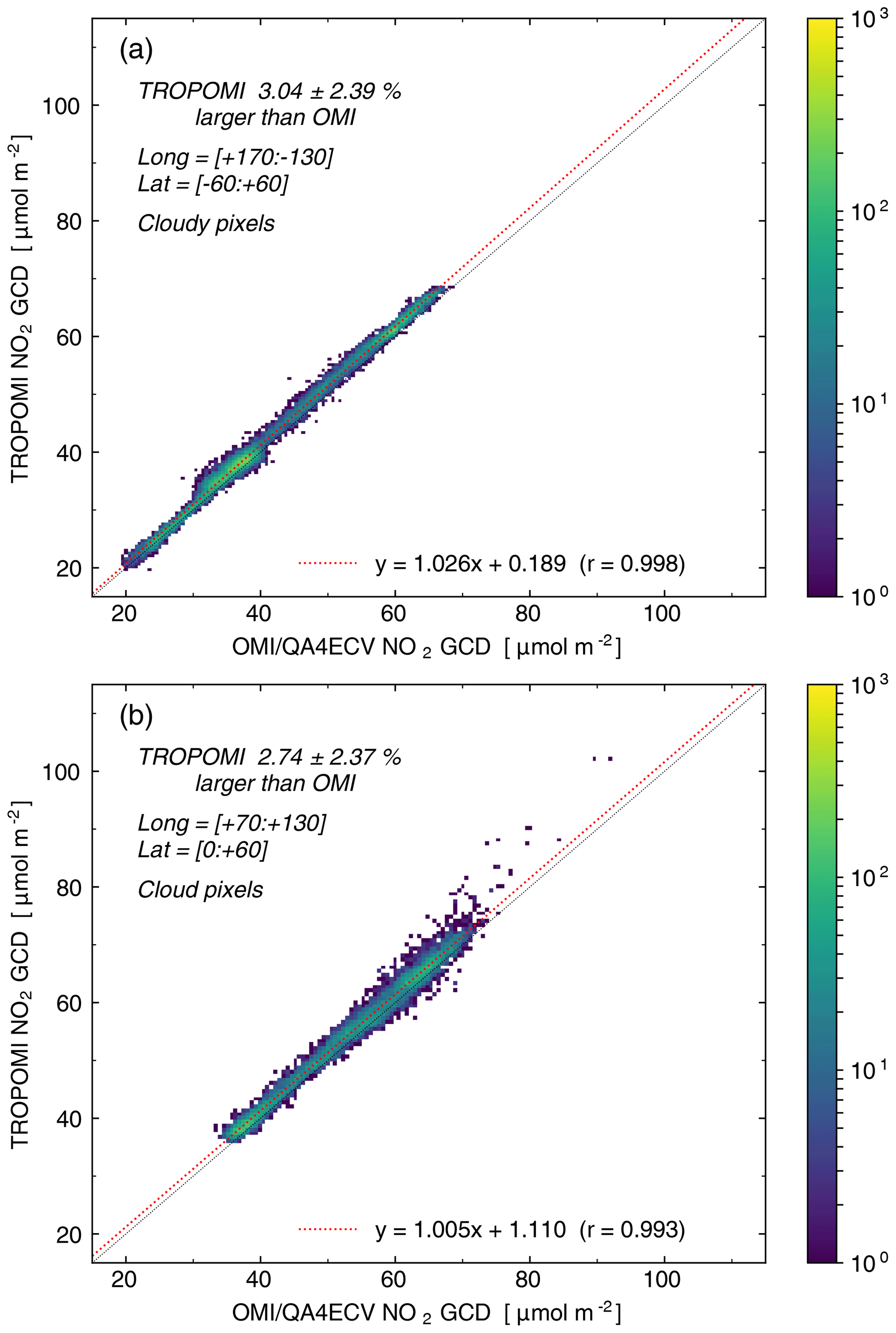
Figure 6 shows the scatter plot of the TROPOMI and OMI/Q4ERCV GCDs of (almost) clear-sky ground pixels (i.e. cloud radiance fraction <0.5) for July 2018 for two regions: the remote Pacific Ocean and the polluted area covering India and China in the Northern Hemisphere; the definition of these two areas is included in the figure panel legends. Both regions show a very good correlation with R2≈0.99. Over the Pacific Ocean area (Fig. 6a) the clear-sky TROPOMI GCD is on average 2.20±1.65 µmol m−2 ( molec. cm−2) or 5.23±3.93 % larger than the OMI–QA4ECV GCD. For January 2019 the result (not shown) is quite similar: the clear-sky TROPOMI GCD over the Pacific Ocean is on average 2.19±1.56 µmol m−2 or 5.78±4.61 % larger than OMI–QA4ECV. Over the polluted India-to-China area (Fig. 6b) the clear-sky TROPOMI GCD is on average 2.02±2.08 µmol m−2 or 3.79±4.06 % larger than OMI–QA4ECV; i.e. the relative difference is a little smaller than from the Pacific Ocean.
For cloudy pixels (i.e. cloud radiance fraction >0.5) the difference between the TROPOMI and OMI–QA4ECV GCD is smaller, both in absolute and in relative terms, and the scatter is less, as can be seen from Fig. 7. Over the Pacific Ocean area (Fig. 7a) the cloudy TROPOMI GCD is on average 1.27±0.93 µmol m−2 ( molec. cm−2) or 3.04±2.39 % larger than the OMI–QA4ECV GCD. Over the polluted India-to-China area (Fig. 7b) the clear-sky TROPOMI GCD is on average 1.38±1.26 µmol m−2 or 2.74±2.37 % larger than OMI–QA4ECV.
These differences between the TROPOMI and the OMI–QA4ECV GCDs (and thus between the SCDs) is comparable to the difference found in Sect. 4.2 due to turning on the intensity offset correction (discussed further in Sect. 5.1) and may therefore be related mainly to the specific settings of the retrieval methods.
4.5 Impact of time difference between radiance and irradiance measurements
In the offline TROPOMI NO2 (re-)processing of a certain radiance orbit, the processor is configured to use the irradiance spectrum measured nearest in time to the radiance orbit. Given that TROPOMI takes irradiance measurements once every 15 orbits (once every ∼25 h and 22 min) and that currently the offline processing is running at least a week after the radiance measurements, the difference in time between the radiance and irradiance measurements will usually be not larger than eight orbits. In this sense, the TROPOMI processing is very different from the OMI processing (whether QA4ECV, OMNO2A or other): for OMI the 2005 average irradiance is used for the full dataset (2004–present) (van Geffen et al., 2015; Zara et al., 2018).
If for the TROPOMI processor one was to use a fixed irradiance, the errors on the retrieval results become larger. Figure 8a illustrates this by showing the across-track TL range average SCD error for radiance orbit 07513 using the irradiance measurement of the same orbit and of orbit 05428 (2085 orbits, 147 d earlier) and of orbit 03058 (4455 orbits, 314 d earlier): the larger the difference in measurement time between radiance and irradiance, the larger the SCD error and the larger the row-to-row variation in the SCD error.
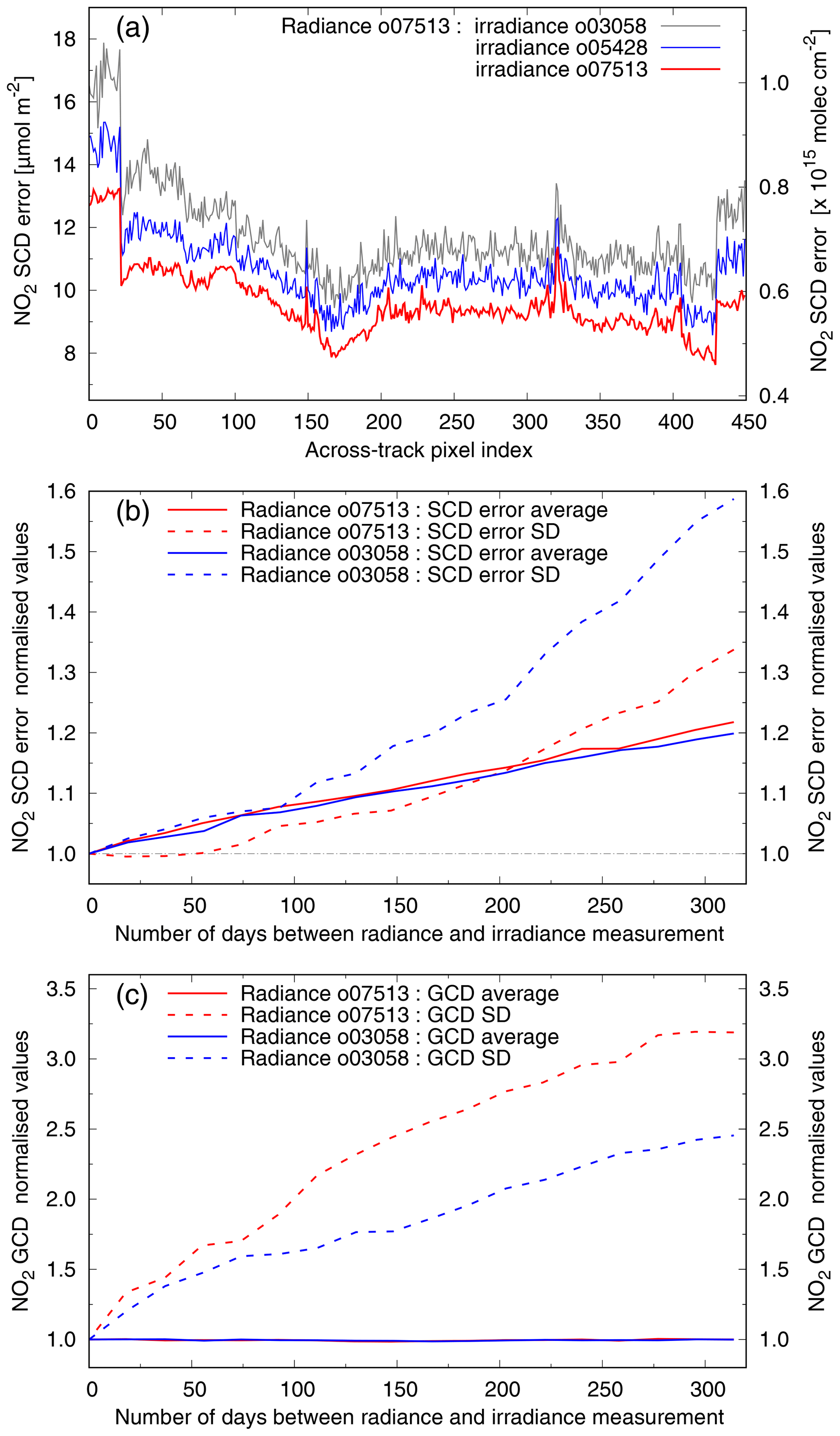
Figure 8Effect of a difference between the radiance and irradiance orbit numbers on the NO2 GCD and the SCD error, averaged over the TL range. (a) SCD error of radiance orbit 07513 (26 March 2019; red) using irradiance measurements from orbits 03058 (16 May 2018; blue), 05428 (30 October 2018; grey) and 07513. (b) SCD error averaged over detector rows 25–424 (solid) and the corresponding standard deviation (dashed) of two radiance orbits (red and blue colours) using a series of irradiance measurements, normalised to 1 for matching orbits, as function of the number of days between radiance and irradiance measurement. (c) Idem for the GCD (solid) and corresponding standard deviation (dashed); note that the two solid GCD curves almost exactly overlap at normalisation value 1.0.
Figure 8b shows the SCD error averaged over detector rows 25–424 (so as to avoid including the higher uncertainties of the outer rows related to the lower on-board pixel binning) and the corresponding standard deviation (SD) for two radiance orbits using selected irradiance measurements from between these two; in the case of radiance orbit 03058 (07513) future (past) irradiances are used. The average SCD error itself increases gradually with increasing time difference, while the SD – a measure of the stripiness of the SCD error – increases more than linearly with time.
For the same series Fig. 8c shows that the average GCD value itself is not affected by the time difference between radiance and irradiance: for radiance orbit 03058 (07513) the average GCD is 41.11±0.18 µmol m−2 (32.79±0.18 µmol m−2). The SD of this averaging – the stripiness of the GCD – increases steeply, levelling off to a factor of around 3. If the TROPOMI processing were to use a fixed irradiance, the de-striping (Sect. 4.3) would show an ever increasing stripe amplitude in Fig. 4c.
It is unclear why the time difference between radiance and irradiance measurements has such a big impact on the TROPOMI NO2 retrieval errors. The solar output varies somewhat over time, but it seems unlikely that this variation is large enough to cause the increase in the retrieval errors. TROPOMI suffers from a small degradation (Rozemeijer and Kleipool, 2019) of 1 %–2 % in the absolute irradiance but with little to no wavelength dependency; hence this degradation is not expected to significantly affect the reflectance and the NO2 SCD retrieval results.
The increased stripiness observed in the OMI NO2 results depicted in Fig. 5, and shown by Boersma et al. (2011) and discussed in detail by Zara et al. (2018), is at least in part the result of the increasing difference in time between radiance and irradiance measurement, but acting over a longer timescale than the effect seen in Fig. 8b and c for TROPOMI. The fact that the GCD value itself (Fig. 8c) is not appreciably affected by the time difference is very reassuring, both for the TROPOMI and the OMI–QA4ECV retrieval results.
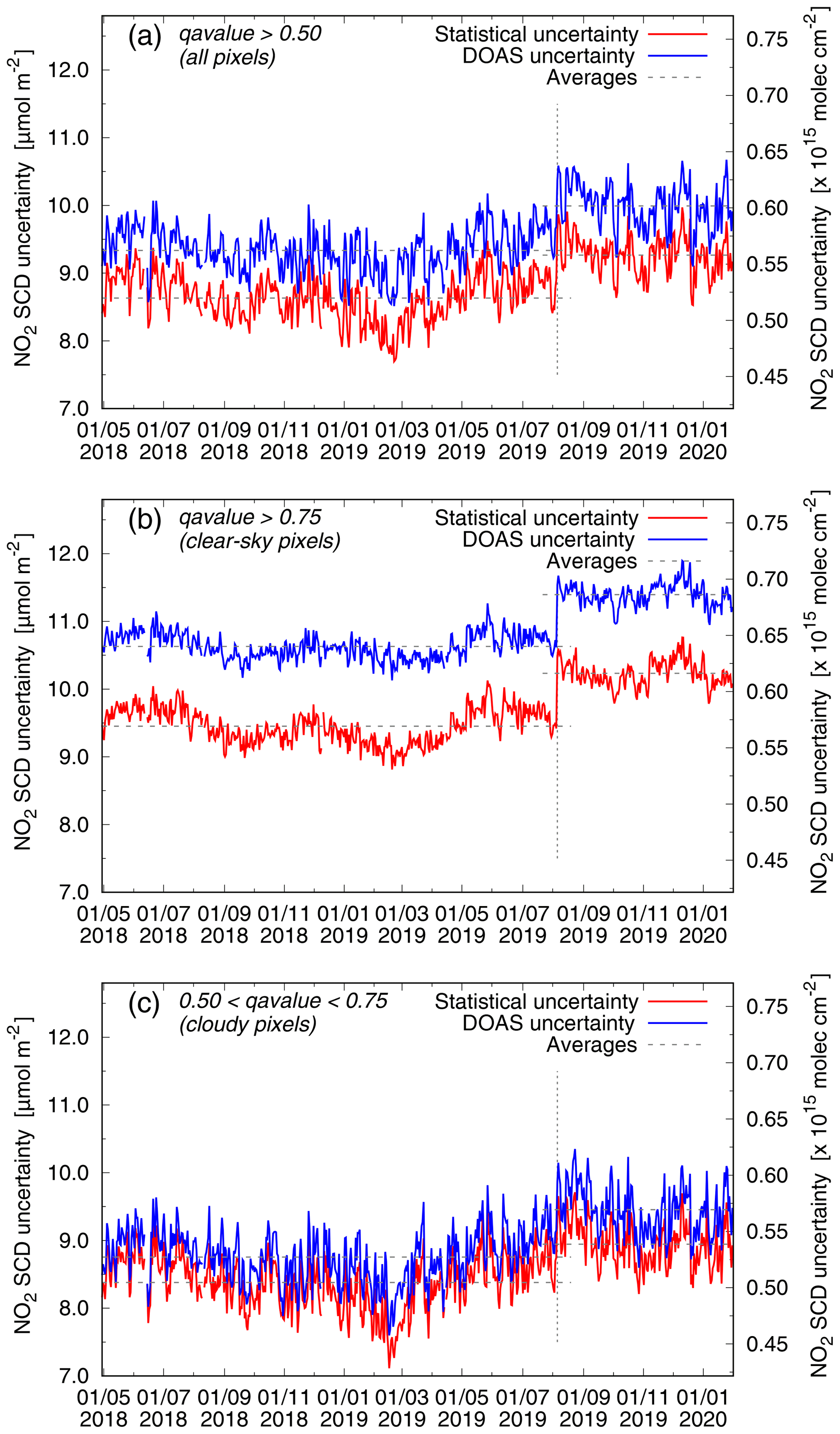
Figure 9NO2 SCD statistical uncertainties (red) and SCD error estimates from the DOAS fit (blue) as function of time. (a) All pixels with successful retrieval. (b) Pixels with cloud radiance fraction <0.5. (c) Pixels with cloud radiance fraction >0.5. The vertical dotted line marks 6 August 2019, when the along-track ground pixel size was reduced. Averages, marked by dashed lines, are listed in Table 3.
4.6 Time dependence of the slant column uncertainty
The spatial variability of the SCDs over a remote Pacific Ocean sector can be used as an independent statistical estimate of the random component of the SCD uncertainty. This approach was used in the QA4ECV project by Zara et al. (2018) to compare OMI and GOME-2A NO2 and formaldehyde SCD values retrieved by different retrieval groups, as well as to compare the SCD error estimates following from the different DOAS fits.
Figure 9 shows the NO2 SCD statistical uncertainties (red) and SCD error estimates from the DOAS fit (blue) as function of time for all ground pixels for which the retrieval was successful (i.e. with quality assurance value 𝚚𝚊_𝚟𝚊𝚕𝚞𝚎>0.50; panel a), for clear-sky pixels (𝚚𝚊_𝚟𝚊𝚕𝚞𝚎>0.75, corresponding to cloud radiance fraction <0.5; panel b), and for cloudy pixels (; panel c). For this exercise the Pacific Ocean orbits (Sect. 2.1.2) were evaluated over the latitude range . Averages over the data period shown in Fig. 9 are listed in Table 3, along with the OMI–QA4ECV results from Zara et al. (2018), who also showed that the OMI–QA4ECV SCD statistical uncertainties and SCD error estimates have increased over the years by about 1 % and 2 % per year, respectively.
Table 3NO2 SCD statistical and SCD DOAS fit uncertainties, averaged over the listed period, given in two units; cf. Fig. 9.
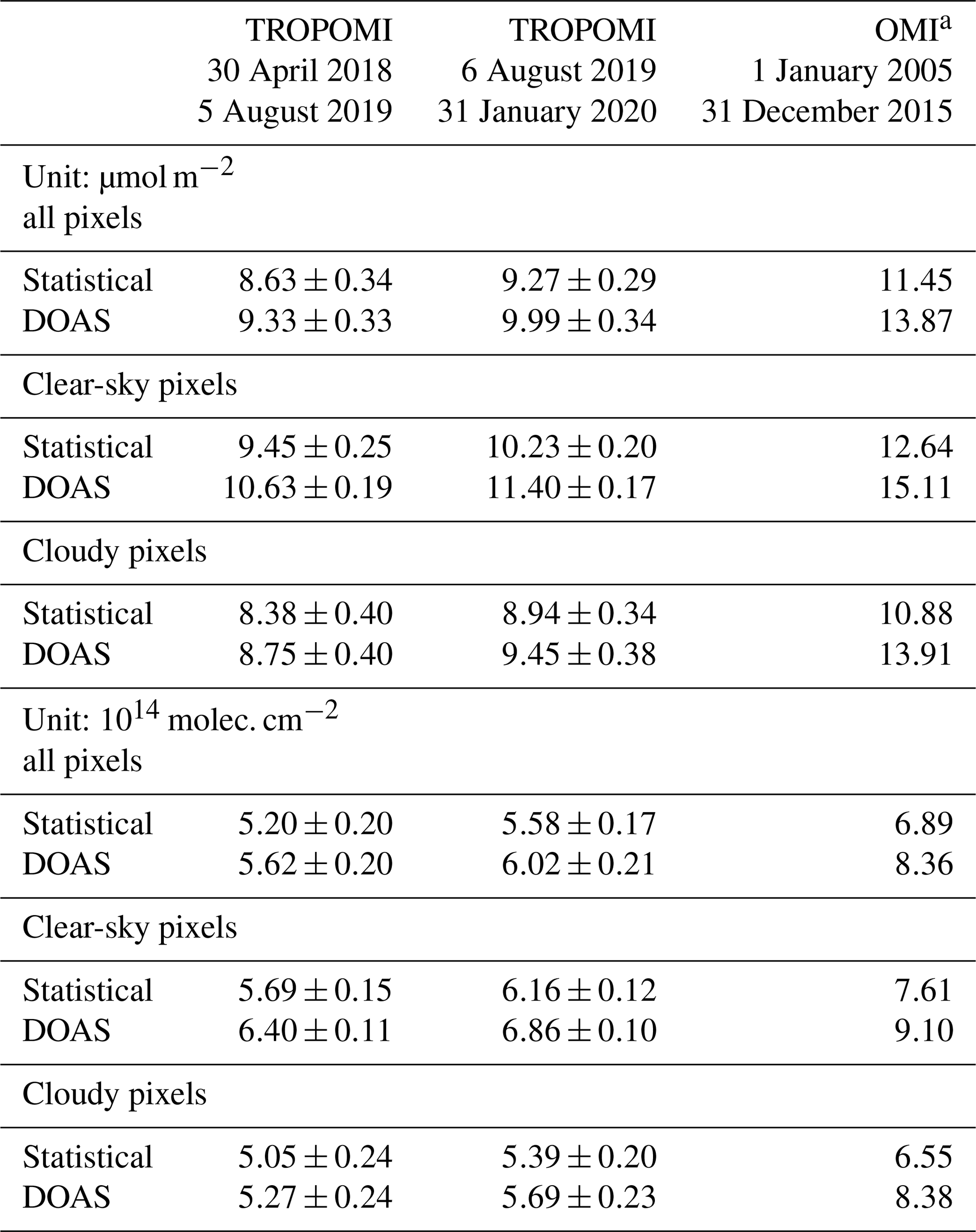
a OMI–QA4ECV results taken from Zara et al. (2018), Table 4; additional data
provided by the author.
The reduction in the along-track ground-pixels size from 7.2 km to 5.6 km on 6 August 2019 effectively entails a reduction in the integration time from 1.08 to 0.84 s, as a result of which the per-pixel noise on the level-1b radiances data increased by a factor of , which in turn caused an increase in the NO2 SCD error by somewhat less than 13 % (because the SCD error is not solely determined by the noise on the radiance spectra). This increase in the SCD error is visible in Fig. 9 as a jump at that date (marked by a vertical dotted line) and is reflected in the averages given in Table 3: the DOAS uncertainty increases by 7 –8%, depending on the pixel type. The pixel size change does not impact the average magnitude of the NO2 GCD (except for polluted regions where due to the smaller pixels size larger peak values may be expected), but it does have an effect on the inter-pixel variation of the GCD: the statistical uncertainty increases by 7%–8%.
All in all, the TROPOMI statistical uncertainties are clearly much lower than those of OMI–QA4ECV, even after the ground pixel size reduction. The SCD error estimates from the DOAS fit routine are on average larger than the statistical uncertainties (for TROPOMI about 10 % and for OMI–QA4ECV about 20 %). From the TROPOMI data it appears that the SCD uncertainty is only about 5 % larger than the statistical uncertainty in the case of cloudy pixels but about 12 % in the case of clear-sky pixels. The main reason for the difference between the DOAS and statistical uncertainties is that, unlike the statistical uncertainties, the SCD error estimates also include systematic retrieval issues, and these appear to play a larger role for clear-sky pixels, i.e. pixels for which the radiance signal is lowest.
From Fig. 9 and Table 3 it is furthermore clear that the statistical and the DOAS uncertainties of TROPOMI appear to be stable over the currently available data period: the standard deviation of the quantities given in Table 3 are small and Fig. 9 shows no systematic change over time. The jumps in the quantities on 6 August 2019 are caused by the along-track pixel size change, not by an instrumental issue, and this change has not affected the stability: the standard deviations of the quantities given in Table 3 are not markedly different between the two measurement modes.
5.1 Intensity offset correction
Many DOAS applications, including the OMI–QA4ECV processing, include a correction for an intensity offset in the radiance, e.g. in the form given in Eq. (9). The precise physical origin of such an intensity offset is not specified in the literature, but it is thought to be related to instrumental issues (e.g. incomplete removal of stray light or dark current in level-1b spectra) and/or atmospheric issues (e.g. incomplete removal of Ring spectrum structures, vibrational Raman scattering (VRS) in clear ocean waters); see, for example, Platt and Stutz (2008), Richter et al. (2011), Peters et al. (2014) and Lampel et al. (2015).
From OMI–QA4ECV evaluations (Müller et al., 2016; Boersma et al., 2018) and a preliminary study using TROPOMI data (Oldeman, 2018), it appears that the largest impact of the intensity offset correction occurs over clear-sky clear ocean water (i.e. with little to no chlorophyll). If indeed absorption by VRS is the key aspect here, it would on physical grounds be more appropriate to include a VRS absorption spectrum (σVRS) in the DOAS fit because the intensity offset corrections are proportional to the irradiance, while σVRS has a different spectral structure; i.e. an intensity offset correction will not fully compensate for VRS absorption. Investigating this matter further falls outside the scope of the present paper.
Turning on the intensity offset correction (IOC) in QDOAS for the TROPOMI and OMI orbits shown in Fig. 3 reduces the GCD values on average by ∼5 %, with the relative impact largest for the lower GCDs. Since this decrease in the GCDs is comparable for both TROPOMI and OMI data, when using the same SCD processor, it seems unlikely that the IOC is correcting for instrumental effects. The quantitative comparison discussed in Sect. 4.4 revealed that for clear-sky cases (Fig. 6) the differences are a little larger than for the cloudy cases (Fig. 7), and for clear-sky cases the difference is larger for the remote Pacific Ocean area (almost completely water) than for the polluted India-to-China area (mainly land surface), while for the cloudy cases the differences are comparable for the two areas. These differences thus seem to indicate that the IOC may be correcting for some absorption effects in ocean waters, but not only for such absorption effects given that the reduction in GCD is also seen over land and over clouds.
It must be noted that the effect of the IOC in QDOAS (viz. Eq. 9) on the GCDs is nearly twice as large as the effect of the experimental IOC in the TROPOMI processor (viz. Eq. 10); apparently these two implementations of the IOC do not behave exactly the same.
All in all an intensity offset correction will not be included in the regular TROPOMI NO2 processing, also because instrumental effects such as stray light and dark current are corrected for in the spectral calibration in the level 0 to 1b processor (Kleipool et al., 2018; Ludewig et al., 2020)
5.2 Validation of stratospheric NO2
Routine validation of TROPOMI data products is being carried out by the Validation Data Analysis Facility (VDAF; http://mpc-vdaf.tropomi.eu/, last access: 17 March 2020), with support from the S5P Validation Team (S5PVT), which issues quarterly validation reports, such as Lambert et al. (2019). Since NO2 over the Pacific Ocean, i.e. away from anthropogenic sources of NO2, is primarily located in the stratosphere, validation of stratospheric NO2 can also be seen as validation of Pacific Ocean NO2 SCDs.
Stratospheric NO2 column data are compared to reference measurements from zenith-sky light (ZSL) DOAS instruments, which are operated in the context of the Network for the Detection of Atmospheric Composition Change (NDACC). ZSL-DOAS measurements, obtained twice daily at twilight, are adjusted to the TROPOMI overpass time in order to account for the diurnal cycle of NO2. Quoting the fifth quarterly report (Lambert et al., 2019), the TROPOMI stratospheric NO2 columns are “generally lower by approximately 0.15×10¹⁵ molec cm−2 [2.5 µmol m−2] than the NDACC ZSL-DOAS ground-based measurements, deployed at 19 stations from pole to pole. The bias of roughly −10 % is within the S5P mission requirements, which is equivalent to 0.2–0.4×10¹⁵ molec cm−2, depending on latitude and season”. The −10 % bias mentioned is the average bias; the median bias is about −7 %. Note that the ZSL-DOAS measurements have their own uncertainties (a bias of at most 10 % and a random uncertainty better than 1 %; Lambert et al., 2019) and that the interpolation to the TROPOMI overpass time introduces uncertainties in the ground-based data of the order of 10 % (Lambert et al., 2019; see also Dirksen et al., 2011).
In other words: the agreement between stratospheric NO2 of TROPOMI and ground-based instruments is rather good, where TROPOMI seems to give SCD column values that are slightly too low. Including an intensity offset correction in the DOAS fit (Sect. 5.1) would lead to a reduction in the Pacific Ocean NO2 SCD by a few percent (Sect. 4.2), which in turn would imply worsening of the validation results.
5.3 NO2 retrieval over strongly polluted areas
In the case NO2 concentrations being no longer optically thin, assumptions lying at the basis of the DOAS retrieval approach may no longer be valid (Richter et al., 2014; Andreas Richter, personal communication, 2019): the relationship between SCD and VCD may become non-linear for single wavelengths, the AMF of boundary layer NO2 may become strongly wavelength dependent and decrease with increasing NO2 columns, and the temperature dependence of the NO2 reference spectrum (usually corrected for a posteriori in the AMF application) may be wavelength dependent. During a dramatic pollution episode in China in January 2013, with NO2 up to 1×10¹⁷ molec. cm−2 (1660 µmol m−2), these effects seemed to become significant, as shown by Richter et al. (2014).
When measuring NO2 over strongly polluted areas with high spatial resolution, such as provided by TROPOMI, the chance of detecting very large NO2 concentrations for individual ground pixels increases. The area with the largest NO2 columns is probably China, but since the reductions in air pollution in China over the past years, it is currently unlikely to encounter NO2 concentrations that are not optically thin in the TROPOMI data, except in a few individual pixels.
NO2 concentrations over China are highest in winter. In January 2019, for example, the highest GCD found over China is 701±16 µmol m−2 in orbit 06637 (24 January), which has 577 pixels (0.05 % of the 1 204 367 pixels with a successful retrieval) with a GCD exceeding 300 µmol m−2; 73 pixels have a GCD values exceeding 400 µmol m−2. Orbit 06580 (20 January) has in that month the largest number of pixels with a GCD exceeding 300 µmol m−2, namely 1609, with a peak value of 512±14 µmol m−2; 256 pixels have GCD values exceeding 400 µmol m−2.
This paper documents the NO2 SCD retrieval method in use for TROPOMI measurements and discusses the stability and uncertainties of the retrieval results. The SCD is key input to the next steps in the NO2 processing chain: the determination of the tropospheric and stratospheric NO2 vertical column densities. Knowledge of the quality and the stability of the SCD retrieval results is therefore important in itself.
The TROPOMI NO2 SCD retrieval describes the modelled reflectance in terms of a non-linear function of the relevant reference spectra and uses optimal estimation to minimise the difference between the measured and modelled reflectance. The results of this retrieval method compare very well with SCD retrievals performed with the QDOAS software (Danckaert et al., 2017) when using settings as close as possible to those of the TROPOMI processor.
The SCD statistical uncertainty originating from the local variability of the SCD over the Pacific Ocean (a remote, source-free region) and the uncertainty estimate following from the DOAS retrieval are quite stable over time. The TROPOMI statistical uncertainties are lower by about 30 % (20 % since the ground pixel size reduction on 6 August 2019) than those of OMI–QA4ECV (Zara et al., 2018), and the SCD error estimates from the DOAS fit routine are on average larger than the statistical uncertainties: for TROPOMI about 10 %, but for OMI–QA4ECV about 20 %. The along-track pixel size reduction from 7.2 to 5.6 km on 6 August 2019 has resulted in an increase in the DOAS and statistical uncertainties by about 8 %.
Quantitative comparison with OMI–QA4ECV data (i.e. OMI measurements processed within the QA4ECV project; Boersma et al., 2018) over the full Pacific Ocean shows very good agreement with a correlation coefficient of about 0.99. TROPOMI values are, however, about 5 µmol m−2 or 5 % higher than the OMI–QA4ECV values, which seems to be due mainly to the fact that the OMI–QA4ECV processing includes a so-called intensity offset correction, which is not applied in the TROPOMI processing: the retrieval of TROPOMI data using QDOAS with different settings shows that the intensity offset correction reduces the SCDs by 4.5 %–5.0 %.
Since NO2 over the Pacific Ocean is primarily stratospheric NO2, validation of stratospheric NO2 essentially is also validation of Pacific Ocean NO2 SCDs. As reported by Lambert et al. (2019), TROPOMI stratospheric columns are lower than ground-based measurements by about 2.5 µmol m−2 (0.15×10¹⁵ molec. cm−2). Since the introduction of an intensity offset correction reduces the SCD by a few percent, it would thus worsen the validation result. Because the physical nature of such an intensity offset is unclear, there are no plans to include an intensity offset correction in future updates of the TROPOMI NO2 SCD retrieval.
The non-physical row-to-row variation (stripe amplitude) of the TROPOMI SCDs (on average 2.15 µmol m−2) is much lower than in the case of OMI–QA4ECV (in 2005 ∼2 and in 2018 ∼5 times the TROPOMI average), but even so a so-called de-striping of the TROPOMI SCDs is applied.
In view of both the SCD error estimate and the across-track striping of the SCDs, it is essential to use an irradiance spectrum measured as closely as possible in time to the radiance measurement in the DOAS fit: the larger the time difference between these two, the larger the SCD error and the larger the stripiness.
An essential difference between the IF retrieval for TROPOMI and the retrieval with QDOAS, whether in ODF mode or IF mode, is the implementation of the correction for the Ring effect, where the authors believe that the TROPOMI implementation is physically more accurate.
In the case of the TROPOMI retrieval (and OMI retrieval using OMNO2A) the correction is included as a non-linear term in the modelled reflectance – the term between large parentheses in Eq. (2) – which depends on a modelled Ring reference spectrum (Iring) and the measured irradiance (E0).
In the case of QDOAS (and similar retrieval algorithms of other institutes) the correction is included as a linear term in the form of a pseudo-absorber in the modelled reflectance – the last term in Eq. (6) – which depends on a fixed reference spectrum determined from a modelled Ring reference spectrum and a convolved reference irradiance spectrum ( minus a second-order polynomial).
The terms on the right-hand side in Eq. (2) can be written as . Taking the natural logarithm and using a Taylor expansion gives In other words, Eq. (2) reduces to Eq. (6) in the case of x≪1, which is usually the case since is less than 0.075 for most ground pixels, assuming Iring∕E0 and σring are the same.
In terms of the cases listed in Table 2, the retrieval of QDOAS case 3 is closest to the TROPOMI retrieval (case b). For all pixels with valid retrieval , with a correlation coefficient better than 0.999. Absolute differences between the coefficients range from −0.002 to +0.006, with largest differences over ocean areas without clouds; above clouds the differences are a factor of 10 smaller. These differences are probably related to the use of the measured or the modelled irradiance spectrum, but the effect on the fit results seems to be quite small. (Cring results from QDOAS case 1 differ slightly from case 2, with a difference smaller than the difference between case 1 and case b.)
The rms error of the intensity fit, given in Eq. (4), and of the optical density fit, Eq. (8), are defined differently, but a first-order relationship between the two can be derived as follows (Andreas Richter, personal communication, 2019).
For good fits the ratio and since for , the summation in Eq. (8) can be rewritten as For not too strongly varying modelled reflectances this can be approximated by With this, the ratio between the rms values of the two methods is since the root mean square of the modelled reflectance can be approximated by the average modelled reflectance.
For the ground pixels with a good quality fit (qa_value ≥0.5)
of an arbitrary TROPOMI orbit the ratio between the rms values appears to
agree with the average modelled reflectance to within 3.7 %.
In order to remove strong outliers in the DOAS fit residual (caused by, e.g., high-energy particles hitting the CCD detector, variations in the dark current or spectral pixels not correctly flagged in the level-1b data in the case of overexposure due to clouds), a “spike removal” algorithm will be used as of v2.1.0 (cf. Sect. 4.1.3). Spectral pixels with such outliers are removed completely from the measured reflectance and the DOAS fit is redone to provide the final fit parameters, which is not followed by another check on outliers, to avoid ending up in a cycle. Outliers occur only in a small fraction of the ground pixels: usually ∼5 % of the successfully processed ground pixels show one or more outliers in their spectrum, and most of these ground pixels with outliers have less than five spectral pixels showing outliers per ground pixel; the largest effects occur over the South Atlantic Anomaly (where the impact of high-energy particles on the detector occurs frequently; cf. Richter et al., 2011) and over bright clouds (where saturation occurs frequently). Hence, the results presented in this paper are not expected to change significantly by the introduction of the spike removal.
The algorithm implemented in the NO2 SCD retrieval for the removal of outliers in the fit residual (van Geffen et al., 2020, Appendix F) uses the box-plot method;3, which determines lower and upper values based on the first and third quartiles: Q1 and Q3, i.e. the 25th and 75th percentile of a distribution (the second quartile, Q2, is the median). If a certain value is larger than or lower than , with the interquartile range and Qf a suitable multiplication factor, it is termed an outlier. The so-called inner and outer fences have Qf=1.5 and Qf=3.0, respectively. For the TROPOMI NO2 SCD v2.1.0 retrieval the outer fences will be used as criterion for outlier detection.
Sources of standard level-1b and level-2 TROPOMI and OMI–QA4ECV data used are listed in Table 1.
JvG conducted the research described in this paper and is responsible for the text. MS and MtL implemented and tested the retrieval code in the TROPOMI processor. HE and KFB are responsible for the final NO2 data product. MZ has been involved in the uncertainty estimates. JPV has been involved in retrieval issues and is the PI of TROPOMI.
The authors declare that they have no conflict of interest.
This article is part of the special issue “TROPOMI on Sentinel-5 Precursor: first year in operation (AMT/ACP inter-journal SI)”. It is not associated with a conference.
The authors would like to thank the following people for discussions on retrieval issues: Piet Stammes, Johan de Haan, Andreas Richter, Steffen Beirle, Michel Van Roozendael and Sergey Marchenko as well as the following people for discussions on level-1b issues: Quintus Kleipool, Nico Rozemeijer, Antje Ludewig and Erwin Loots. We further would like to thank the three anonymous referees for their suggestions for improvements. Sentinel-5 Precursor is a European Space Agency (ESA) mission on behalf of the European Commission (EC). The TROPOMI payload is a joint development by ESA and the Netherlands Space Office (NSO). The Sentinel-5 Precursor ground-segment development has been funded by ESA and with national contributions from the Netherlands, Germany and Belgium. Contains modified Copernicus Sentinel data 2018–2019.
This paper was edited by Ben Veihelmann and reviewed by three anonymous referees.
Beirle, S., Boersma, K. F., Platt, U., Lawrence, M. G., and Wagner T.: Megacity emissions and lifetimes of nitrogen oxides probed from space, Science, 333, 1737–1739, https://doi.org/10.1126/science.1207824, 2011. a
Babić, L., Braak, R., Dierssen, R., Kissi-Ameyaw, J., Kleipool, J., Leloux, J., Loots, E., Ludewig, A., Rozemeijer, N., Smeets, S., and Vacanti, G.: Algorithm theoretical basis document for the TROPOMI L01b data processor, Report S5P-KNMI-L01B-0009-SD, issue 8.0.0, 1 June 2017, KNMI, De Bilt, the Netherlands, available at: http://www.tropomi.eu/documents/level-0-1b (last access: 17 March 2020), 2017. a
Boersma, K. F., Eskes, H. J., Veefkind, J. P., Brinksma, E. J., van der A, R. J., Sneep, M., van den Oord, G. H. J., Levelt, P. F., Stammes, P., Gleason, J. F., and Bucsela, E. J.: Near-real time retrieval of tropospheric NO2 from OMI, Atmos. Chem. Phys., 7, 2103–2118, https://doi.org/10.5194/acp-7-2103-2007, 2007. a, b
Boersma, K. F., Eskes, H. J., Dirksen, R. J., van der A, R. J., Veefkind, J. P., Stammes, P., Huijnen, V., Kleipool, Q. L., Sneep, M., Claas, J., Leitão, J., Richter, A., Zhou, Y., and Brunner, D.: An improved tropospheric NO2 column retrieval algorithm for the Ozone Monitoring Instrument, Atmos. Meas. Tech., 4, 1905–1928, https://doi.org/10.5194/amt-4-1905-2011, 2011. a, b, c
Boersma, K. F., Eskes, H. J., Richter, A., De Smedt, I., Lorente, A., Beirle, S., van Geffen, J. H. G. M., Zara, M., Peters, E., Van Roozendael, M., Wagner, T., Maasakkers, J. D., van der A, R. J., Nightingale, J., De Rudder, A., Irie, H., Pinardi, G., Lambert, J.-C., and Compernolle, S. C.: Improving algorithms and uncertainty estimates for satellite NO2 retrievals: results from the quality assurance for the essential climate variables (QA4ECV) project, Atmos. Meas. Tech., 11, 6651–6678, https://doi.org/10.5194/amt-11-6651-2018, 2018. a, b, c, d, e, f
Bovensmann, H., Burrows, J. P., Buchwitz, M., Frerick, J., Noel, S., Rozanov, V. V., Chance, K. V., and Goede, A. P. H.: SCIAMACHY: Mission objectives and measurement modes, J. Atmos. Sci., 56, 127–150, 1999. a
Burrows, J. P., Weber, M., Buchwitz, M., Rozanov, V., Ladstätter-Weißenmayer, A., Richter, A., Debeek, R., Hoogen, R., Bramstedt, K., Eichmann, K.-U., Eisinger, M., and Perner, D.: The Global Ozone Monitoring Experiment (GOME): Mission concept and first results, J. Atmos. Sci., 56, 151–175, 1999. a
Chance, K. V. and Spurr, R. J. D.: Ring effect studies: Rayleigh scattering, including molecular parameters for rotational Raman scattering, and the Fraunhofer spectrum, Appl. Optics, 36, 5224–5230, 1997. a, b
Crutzen, P. J.: The influence of nitrogen oxides on the atmospheric ozone content, Q. J. Roy. Meteor. Soc., 96, 320–325, 1970. a
Danckaert, T., Fayt, C., Van Roozendael, M., De Smedt, I., Letocart, V., Merlaud, A., and Pinardi, G.: QDOAS software user manual, issue 3.2, September 2017, BIRA-IASB, Brussels, Belgium, available at: http://uv-vis.aeronomie.be/software/QDOAS/ (last access: 17 March 2020), 2017. a, b, c, d, e
Dirksen, R. J., Boersma, K. F., Eskes, H. J., Ionov, D. V., Bucsela, E. J., Levelt, P. F., and Kelder, H. M.: Evaluation of stratospheric NO2 retrieved from the Ozone Monitoring Instrument: Intercomparison, diurnal cycle, and trending, J. Geophys. Res. 17, 3972–3981, https://doi.org/10.1029/2010JD014943, 2011. a
Dobber, M., Voors, R., Dirksen, R., Kleipool, Q., and Levelt, P.: The high-resolution solar reference spectrum between 250 and 550 nm and its application to measurements with the Ozone Monitoring Instrument, Sol. Phys., 249, 281–291, https://doi.org/10.1007/s11207-008-9187-7, 2008. a
Eskes, H. J. and Eichmann K.-U.: S5P MPC Product Readme Nitrogen Dioxide, Report S5P-MPC-KNMI-PRF-NO2, version 1.4, 6 August 2019, ESA, available at: http://www.tropomi.eu/documents/prf/, 17 March 2020. a
Eskes, H. J, van Geffen, J. H. G. M., Boersma, K. F., Eichmann K.-U.. Apituley, A., Pedergnana, M., Sneep, M., Veefkind, J. P., and Loyola, D.: S5P/TROPOMI Level-2 Product User Manual Nitrogen Dioxide, Report S5P-KNMI-L2-0021-MA, version 3.0.0, 27 March 2019, ESA, available at: http://www.tropomi.eu/documents/pum/, last access: 17 March 2020. a
Eskes, H. et al.: S5P/TROPOMI NO2 vertical column retrieval Atmos. Meas. Tech., in preparation, 2020. a
Fuglestvedt, J. S., Berntsen, T., Isaksen, I. S. A., Mao, H., Liang, X.-Z., and Wang, W.-C.: Climatic forcing of nitrogen oxides through changes in tropospheric ozone and methane, Atmos. Environ., 33, 961–977, https://doi.org/10.1016/s1352-2310(98)00217-9, 1999. a
Grainger, J. F. and Ring, J.: Anomalous Fraunhofer line profiles, Nature, 193, 762, https://doi.org/10.1038/193762a0, 1962. a
Hendrick, F., Mahieu, E., Bodeker, G. E., Boersma, K. F., Chipperfield, M. P., De Mazière, M., De Smedt, I., Demoulin, P., Fayt, C., Hermans, C., Kreher, K., Lejeune, B., Pinardi, G., Servais, C., Stübi, R., van der A, R., Vernier, J.-P., and Van Roozendael, M.: Analysis of stratospheric NO2 trends above Jungfraujoch using ground-based UV-visible, FTIR, and satellite nadir observations, Atmos. Chem. Phys., 12, 8851–8864, https://doi.org/10.5194/acp-12-8851-2012, 2012. a
Kleipool, Q., Ludewig, A., Babić, L., Bartstra, R., Braak, R., Dierssen, W., Dewitte, P.-J., Kenter, P., Landzaat, R., Leloux, J., Loots, E., Meijering, P., van der Plas, E., Rozemeijer, N., Schepers, D., Schiavini, D., Smeets, J., Vacanti, G., Vonk, F., and Veefkind, P.: Pre-launch calibration results of the TROPOMI payload on-board the Sentinel-5 Precursor satellite, Atmos. Meas. Tech., 11, 6439–6479, https://doi.org/10.5194/amt-11-6439-2018, 2018. a
Lambert, J.-C., Keppens, A., Hubert, D., Langerock, B., Eichmann, K.-U., Kleipool, Q., Sneep, M., Verhoelst, T., Wagner, T., Weber, M., Ahn, C., Argyrouli, A., Balis, D., Chan, K. L., Compernolle, S., De Smedt, I., Eskes, H., Fjæraa, A. M., Garane, K., Gleason, J. F., Goutail, F., Granville, J., Hedelt, P., Heue, K.-P., Jaross, G., Koukouli, M.-L., Landgraf, J., Lutz, R., Niemejer, S., Pazmiño, A., Pinardi, G., Pommereau, J.-P., Richter, A., Rozemeijer, N., Sha, M.K., Stein Zweers, D., Theys, N., Tilstra, G., Torres, O., Valks, P., Vigouroux, C., and Wang, P.: Quarterly Validation Report of the Copernicus Sentinel-5 Precursor Operational Data Products, #05: April 2018–November 2019, S5P MPC Routine Operations Consolidated Validation Report series, Issue #05, Version 05.0.1, 151 pp., December 2019, available at: http://mpc-vdaf.tropomi.eu/index.php/nitrogen-dioxide/ (last access: 17 March 2020), 2019. a, b, c, d, e, f
Lampel, J., Frieß, U., and Platt, U.: The impact of vibrational Raman scattering of air on DOAS measurements of atmospheric trace gases, Atmos. Meas. Tech., 8, 3767–3787, https://doi.org/10.5194/amt-8-3767-2015, 2015. a
Levelt, P. F., van den Oord, G. H. J., Dobber, M. R. Dobber, Mälkki, A., Visser, H., de Vries, J., Stammes, P., Lundell, J. O. V., and Saari, H.: The Ozone Monitoring Instrument, IEEE Trans. Geosci. Rem. Sens., 44, 1093–1101, https://doi.org/10.1109/tgrs.2006.872333, 2006. a, b
Levelt, P. F., Joiner, J., Tamminen, J., Veefkind, J. P., Bhartia, P. K., Stein Zweers, D. C., Duncan, B. N., Streets, D. G., Eskes, H., van der A, R., McLinden, C., Fioletov, V., Carn, S., de Laat, J., DeLand, M., Marchenko, S., McPeters, R., Ziemke, J., Fu, D., Liu, X., Pickering, K., Apituley, A., González Abad, G., Arola, A., Boersma, F., Chan Miller, C., Chance, K., de Graaf, M., Hakkarainen, J., Hassinen, S., Ialongo, I., Kleipool, Q., Krotkov, N., Li, C., Lamsal, L., Newman, P., Nowlan, C., Suleiman, R., Tilstra, L. G., Torres, O., Wang, H., and Wargan, K.: The Ozone Monitoring Instrument: overview of 14 years in space, Atmos. Chem. Phys., 18, 5699–5745, https://doi.org/10.5194/acp-18-5699-2018, 2018. a
Ludewig, A., Kleipool, Q., Bartstra, R., Landzaat, R., Leloux, J., Loots, E., Meijering, P., van der Plas, E., Rozemeijer, N., Vonk, F., and Veefkind, P.: In-flight calibration results of the TROPOMI payload on-board theSentinel-5 Precursor satellite, Atmos. Meas. Tech. Discuss., https://doi.org/10.5194/amt-2019-488, in review, 2020. a, b, c, d, e, f, g
Müller, J.-P., Kharbouche, S., Gobron, N., Scanlon, T., Govaerts, Y., Danne, O., Schultz, J., Lattanzio, A., Peters, E., De Smedt, I., Beirle, S., Lorente, A., Coheur, P. F., George, M., Wagner, T., Hilboll, A., Richter, A., Van Roozendael, M., and Boersma, K. F.: Recommendations (scientific) on best practices for retrievals for Land and Atmosphere ECVs (QA4ECV Deliverable 4.2 version 1.0), 186 pp., available at: http://www.qa4ecv.eu/sites/default/files/D4.2.pdf, last access: 17 March 2020), 2016. a
Munro, R., Eisinger, M., Anderson, C., Callies, J., Corpaccioli, E. Lang, R., Lefebvre, A., Livschitz, Y., and Albinana, A. P.: GOME-2 on MetOp, ESA publication SP 628, Paris, 2006. a
Munro, R., Lang, R., Klaes, D., Poli, G., Retscher, C., Lindstrot, R., Huckle, R., Lacan, A., Grzegorski, M., Holdak, A., Kokhanovsky, A., Livschitz, J., and Eisinger, M.: The GOME-2 instrument on the Metop series of satellites: instrument design, calibration, and level 1 data processing – an overview, Atmos. Meas. Tech., 9, 1279–1301, https://doi.org/10.5194/amt-9-1279-2016, 2016. a
Murphy, D. M., Fahey, D. W., Proffitt, M. H., Liu, S. C., Chan, K. R., Eubank, C. S., Kawa, S. R., and Kelly, K. K.: Reactive nitrogen and its correlation with ozone in the lower stratosphere and upper troposphere, J. Geophys. Res., 98, 8751–8773, https://doi.org/10.1029/92JD00681, 1993. a
Oldeman, A.: Effect of including an intensity offset in the DOAS NO2 retrieval of TROPOMI, Internship report, R-1944-SE, Eindhoven University of Technology/KNMI, Eindhoven, May 2018, available at: https://kfolkertboersma.files.wordpress.com/2018/06/report_oldeman_22052018.pdf (last access: 17 March 2020), 2018. a
Peters, E., Wittrock, F., Richter, A., Alvarado, L. M. A., Rozanov, V. V., and Burrows, J. P.: Liquid water absorption and scattering effects in DOAS retrievals over oceans, Atmos. Meas. Tech., 7, 4203–4221, https://doi.org/10.5194/amt-7-4203-2014, 2014. a
Platt, U.: Differential Optical Absorption Spectroscopy (DOAS), in: Air monitoring by spectroscopic techniques, edited by: Sigrist, M. W., Chemical Analisys Series, 127, 27–76, Wiley, New York, 1994. a
Platt, U. and Stutz, Z.: Differential Optical Absorption Spectroscopy, Principles and Applications, Springer, Heidelberg, Germany, 597 pp., 2008. a, b
Pope, R. M. and Fry, E. S.: Absorption spectrum (380–700 nm) of pure water. II. Integrating cavity measurements, Appl. Optics, 36, 8710–8723, https://doi.org/10.1364/AO.36.008710, 1997. a
Press, W. H., Teukolsky, S. A., Vetterling,W. T., and Flannery, B. P.: Numerical recipes in Fortran 77: The art of scientific computing, Cambridge University Press, 2nd edn., New York, USA, 1997. a, b
Richter, A., Begoin, M., Hilboll, A., and Burrows, J. P.: An improved NO2 retrieval for the GOME-2 satellite instrument, Atmos. Meas. Tech., 4, 1147–1159, https://doi.org/10.5194/amt-4-1147-2011, 2011. a, b
Richter, A., Hilboll, A., and Burrows, J. P.: Improving satellite retrievals of large tropospheric NO2 columns, Geophys. Res. Abstr. 16, EGU General Assembly 2014, EGU2014-11669, 2014. a, b
Rodgers, C. D.: Inverse Methods for Atmospheric Sounding: Theory and Practice, World Scientific Publishing, London, UK, 2000. a, b
Rothman, L. S., Gordon, I. E., Babikov, Y., Barbe, A., Chris Benner, D., Bernath, P. F., Birk, M., Bizzocchi, L., Boudon, V., Brown, L. R., Campargue, A., Chance, K., Cohen, E. A., Coudert, L. H., Devi, V. M., Drouin, B. J., Fayt, A., Flaud, J.-M., Gamache, R. R., Harrison, J. J., Hartmann, J.-M., Hill C., Hodges, J. T., Jacquemart, D., Jolly, A., Lamouroux, J., Le Roy, R. J., Li, G., Long, D. A., Lyulin, O. M., Mackie, C. J., Massie, S. T., Mikhailenko, S., Müller, H. S. P., Naumenko, O. V., Nikitin, A. V., Orphal, J., Perevalov, V., Perrin, A., Polovtseva, E. R., Richard, C., Smith, M. A. H., Starikova, E., Sung, K., Tashkun, S., Tennyson, J., Toon, G. C., Tyuterev, Vl. G., and Wagn, G.: The HITRAN 2012 molecular spectroscopic database, J. Quant. Spectrosc. Ra., 130, 4–50, https://doi.org/10.1016/j.jqsrt.2013.07.002, 2013. a
Rozemeijer, N. and Kleipool, Q.: S5P Mission Performance Centre Level 1b Readme Report S5P-MPC-KNMI-PRF-L1B, issue 1.0.0, 10 July 2018 KNMI, De Bilt, the Netherlands, available at: http://www.tropomi.eu/documents/level-0-1b, last access: 17 March 2020. a, b, c
Schaub, D., Brunner, D., Boersma, K. F., Keller, J., Folini, D., Buchmann, B., Berresheim, H., and Staehelin, J.: SCIAMACHY tropospheric NO2 over Switzerland: estimates of NOx lifetimes and impact of the complex Alpine topography on the retrieval, Atmos. Chem. Phys., 7, 5971–5987, https://doi.org/10.5194/acp-7-5971-2007, 2007. a
Schenkeveld, V. M. E., Jaross, G., Marchenko, S., Haffner, D., Kleipool, Q. L., Rozemeijer, N. C., Veefkind, J. P., and Levelt, P. F.: In-flight performance of the Ozone Monitoring Instrument, Atmos. Meas. Tech., 10, 1957–1986, https://doi.org/10.5194/amt-10-1957-2017, 2017. a, b
Seinfeld, J. H. and Pandis, S. N.: Atmospheric Chemistry and Physics – From Air Pollution to Climate Change (2nd Edition), John Wiley & Sons, Hoboken, New Jersey, USA, 2006. a
Serdyuchenko, A., Gorshelev, V., Weber, M., Chehade, W., and Burrows, J. P.: High spectral resolution ozone absorption cross-sections – Part 2: Temperature dependence, Atmos. Meas. Tech., 7, 625–636, https://doi.org/10.5194/amt-7-625-2014, 2014. a
Shindell, D. T., Faluvegi, G., Koch, D. M., Schmidt, G. A., Unger, N., and Bauer, S. E.: Improved attribution of climate forcing to emissions, Science, 326, 716–718, https://doi.org/10.1126/science.1174760, 2009. a
Sillman, S., Logan, J. A., and Wofsy, S. C.: The sensitivity of ozone to nitrogen oxides and hydrocarbons in regional ozone episodes, J. Geophys. Res., 95, 1837–1851, https://doi.org/10.1029/JD095iD02p01837 1990. a
Thalman, R. and Volkamer, R.: Temperature dependant absorption cross-sections of O2−O2 collision pairs between 340 and 630 nm at atmospherically relevant pressure Phys. Chem. Chem. Phys., 15, 15371–15381, https://doi.org/10.1039/C3CP50968K, 2013. a
van der A, R. J., Mijling, B., Ding, J., Koukouli, M. E., Liu, F., Li, Q., Mao, H., and Theys, N.: Cleaning up the air: effectiveness of air quality policy for SO2 and NOx emissions in China, Atmos. Chem. Phys., 17, 1775–1789, https://doi.org/10.5194/acp-17-1775-2017, 2017. a
Vandaele, A. C., Hermans, C., Simon, P. C., Carleer, M., Colin, R., Fally, S., Mérienne, M. F., Jenouvrier, A., and Coquart, B.: Measurements of the NO2 absorption cross-section from 42 000 cm−1 to 10 000 cm−1 (238–1000 nm) at 220 K and 294 K, J. Quant. Spectrosc. Ra., 59, 171–184, https://doi.org/10.1016/S0022-4073(97)00168-4, 1998. a
van Geffen, J. H. G. M., Boersma, K. F., Van Roozendael, M., Hendrick, F., Mahieu, E., De Smedt, I., Sneep, M., and Veefkind, J. P.: Improved spectral fitting of nitrogen dioxide from OMI in the 405–465 nm window, Atmos. Meas. Tech., 8, 1685–1699, https://doi.org/10.5194/amt-8-1685-2015, 2015. a, b, c, d
van Geffen, J. H. G. M., Eskes, H. J., Boersma, K. F., Maasakkers, J. D., and Veefkind, J. P.: TROPOMI ATBD of the total and tropospheric NO2 data products, Report S5P-KNMI-L2-0005-RP, version 1.4.0, released 6 February 2019, KNMI, De Bilt, the Netherlands, available at: http://www.tropomi.eu/documents/atbd/, last access: 17 March 2020. a, b, c, d, e
van Geffen, J. H. G. M., Eskes, H. J., Boersma, K. F., Maasakkers, J. D., and Veefkind, J. P.: TROPOMI ATBD of the total and tropospheric NO2 data products, Report S5P-KNMI-L2-0005-RP, version 2.1.0, to be released, KNMI, De Bilt, the Netherlands, available at: http://www.tropomi.eu/documents/atbd/ (last access: 4 December 2019), 2020. a, b
Veefkind, J. P., Aben, I., McMullan, K., Förster, H., de Vries, J., Otter, G., Claas, J., Eskes, H. J., de Haan, J. F., Kleipool, Q., van Weele, M., Hasekamp, O., Hoogeveen, R., Landgraf, J., Snel, R., Tol, P., Ingmann, P., Voors, R., Kruizinga, B., Vink, R., Visser, H., and Levelt, P. F.: TROPOMI on the ESA Sentinel-5 Precursor: A GMES mission for global observations of the atmospheric composition for climate, air quality and ozone layer applications, Remote Sens. Environ., 120, 70–83, https://doi.org/10.1016/j.rse.2011.09.027, 2012. a, b
Veihelmann, B. and Kleipool, Q.: Reducing Along-Track Stripes in OMI-Level 2 Products, TN-OMIE-KNMI-785, 24 pp., KNMI, De Bilt, the Netherlands, 2006. a
Wang, S. W., Zhang, Q., Streets, D. G., He, K. B., Martin, R. V., Lamsal, L. N., Chen, D., Lei, Y., and Lu, Z.: Growth in NOx emissions from power plants in China: bottom-up estimates and satellite observations, Atmos. Chem. Phys., 12, 4429–4447, https://doi.org/10.5194/acp-12-4429-2012, 2012. a
World Health Organisation: Health Aspects of Air Pollution with Particulate Matter, Ozone and Nitrogen Dioxide, World Health Organisation, Bonn, Germany, 98 pp., 2003. a
Zara, M., Boersma, K. F., De Smedt, I., Richter, A., Peters, E., van Geffen, J. H. G. M., Beirle, S., Wagner, T., Van Roozendael, M., Marchenko, S., Lamsal, L. N., and Eskes, H. J.: Improved slant column density retrieval of nitrogen dioxide and formaldehyde for OMI and GOME-2A from QA4ECV: intercomparison, uncertainty characterisation, and trends, Atmos. Meas. Tech., 11, 4033–4058, https://doi.org/10.5194/amt-11-4033-2018, 2018. a, b, c, d, e, f, g, h
The correlation coefficients, however, are not available in the current TROPOMI data product.
An initially planned new version 2.0.0 will not be deployed.
“What are outliers in the data?” https://www.itl.nist.gov/div898/handbook/prc/section1/prc16.htm (last access: 17 March 2020).
- Abstract
- Introduction
- Satellite data sources and data selection
- NO2 slant column retrieval
- NO2 slant column retrieval evaluation
- Discussion
- Concluding remarks
- Appendix A: Implementation of the Ring correctionin the intensity and optical density fit models
- Appendix B: Relationship between the rms errorin the intensity and optical density fit models
- Appendix C: TROPOMI spike removal
- Data availability
- Author contributions
- Competing interests
- Special issue statement
- Acknowledgements
- Review statement
- References