the Creative Commons Attribution 4.0 License.
the Creative Commons Attribution 4.0 License.
 | 24 Mar 2020
Analysis of flow in complex terrain using multi-Doppler lidar retrievals
Petra Klein
Norman Wildmann
Robert Menke
Strategically placed Doppler lidars (DLs) offer insights into flow processes that are not observable with meteorological towers. For this study we use intersecting range height indicator (RHI) scans of scanning DLs to create four virtual towers. The measurements were performed during the Perdigão experiment, which set out to study atmospheric flows in complex terrain and to collect a high-quality dataset for the validation of meso- and microscale models. Here we focus on a period of 6 weeks from 1 May 2017 through 15 June 2017. During this Intensive Observation Period (IOP) data of six intersecting RHI scans are used to calculate wind speeds at four virtual towers located along the valley at Perdigão with a temporal resolution of 15 min. While meteorological towers were only up to 100 m tall, the virtual towers cover heights from 50 to 600 m above the valley floor. Thus, they give additional insights into the complex interactions between the flow inside the valley and higher up across the ridges. Along with the wind speed and direction, uncertainties of the virtual-tower retrieval were analyzed. A case study of a nighttime stable boundary layer flow with wave features in the valley is presented to illustrate the usefulness of the virtual towers in analyzing the spatially complex flow over the ridges during the Perdigão campaign. This study shows that, despite having uncoordinated scans, the retrieved virtual towers add value in observing flow in and above the valley. Additionally, the results show the virtual towers can more accurately capture the flow in areas where the assumptions for more traditional DL scan strategies break down.


Scanning Doppler lidar (DL) systems have proven to be useful in many different sectors of atmospheric study. They have been used for boundary layer meteorology (Klein et al., 2015; Fernando et al., 2015), wind energy research (Banta et al., 2015; Newman et al., 2016; Choukulkar et al., 2017), and other various fields of study (Sathe and Mann, 2013; Bonin et al., 2017). DLs measure the radial velocity along a beam in a high spatial and temporal resolution. Different scanning strategies can give different insights into the flow field surrounding the DLs. For example, a plan position indicator (PPI) scan gives a representation of the spatial variability in the horizontal by scanning at a fixed elevation and only moving in azimuth, while a range height indicator (RHI) scan essentially gives a cross section of the flow by staying at a fixed azimuth but changing elevation.
By applying assumptions to the flow, one can use these different scan strategies to derive the two-dimensional (2D) and three-dimensional (3D) wind from a single DL. The simplest techniques to derive the wind speed and direction are the velocity azimuth display (VAD) technique (Browning and Wexler, 1968) and the Doppler beam swinging (DBS) technique (Strauch et al., 1984). However, these techniques make the assumption that the wind is horizontally homogeneous in order to retrieve the wind speed and direction; this is often not the case in boundary layer meteorology and can introduce errors into the wind estimates. One area where the assumption of horizontal homogeneity is likely invalid is in the study of complex terrain, where different beams of a scan pattern may sample different flow features. While in flat homogeneous terrain the accuracy of wind speed measurements with conically scanning DLs was found to be within a few percent, in complex terrain errors as large as 10 % are not uncommon (Bingöl et al., 2009; Bradley et al., 2015). Correction techniques such as Leosphere's Flow Complexity Recognition (FCR) algorithm focus on correcting errors introduced by terrain by using simple flow models (see Leosphere, 2020). Other techniques using a single DL have been developed to limit the assumption of horizontal homogeneity (Waldteufel and Corbin, 1979; Wang et al., 2015).
In complex terrain, retrievals using multiple DLs with beams that intersect in the same volume of air may be needed to accurately measure the 3D wind field. By combining multiple different radial wind vectors, one can solve the 3D transformation matrix to get the 3D wind vector without applying any assumptions to the flow. There are multiple ways that this can be done. For example, coplanar RHI scans were used in the Terrain-induced Rotor Experiment to study rotors caused by mountains (Hill et al., 2010), multi-Doppler scan strategies were used in the Perdigão 2015 and 2017 experiments to measure wind turbine wake deficits in highly complex terrain (Barthelmie et al., 2018; Menke et al., 2018; Wildmann et al., 2018a, b), and virtual towers (VTs) were used in the Joint Urban experiment in 2003 (Calhoun et al., 2006).
Multi-Doppler measurements can augment more traditional observation strategies and are highly adaptable to an experiment's science objectives, but they are not perfect. Though some precision is lost due to volumetric averaging, the results are generally accurate to within 0.2 m s−1 (Damian et al., 2014; Pauscher et al., 2016; Debnath et al., 2017). Higher levels of uncertainty have been found with more complicated scan strategies (Choukulkar et al., 2017). For multi-Doppler retrievals, the magnitude of uncertainty was directly related to the ability to precisely coordinate scans (Wildmann et al., 2018b). Additionally, higher levels of uncertainty are present during unstable conditions (Newman et al., 2016).
This study assesses how well traditional methods and 2D and 3D multi-Doppler measurements perform in a complex setting. Additionally, it provides an analysis of terrain-induced uncertainties compared to both multi-Doppler measurements and traditional single-Doppler wind estimation techniques. One challenge was however the fact that all of the techniques applied have limitations, and a true reference dataset for quantifying the measurement errors did not exist. This is further addressed in Sect. 4.1.
The data presented in this study were collected during the Perdigão field campaign during the spring and early summer of 2017, which is one of multiple experiments conducted in order to build the New European Wind Atlas (NEWA) (Mann et al., 2017). As wind energy becomes more popular, the need for models to accurately predict energy output from wind resources becomes increasingly important. NEWA provides a standard dataset of wind energy resources for Europe through the creation of new and improved meso- and microscale models and modeling techniques. One important aspect of developing these modeling techniques is verifying their accuracy against high-quality datasets. Therefore, one of the main goals in the creation of the NEWA is developing new modeling methodologies which have been tested against observations from various measurement campaigns conducted in different landscapes and climates.
To validate numerical models, detailed measurements of the flow at multiple scales are required (Banta et al., 2013; Fernando et al., 2015). To this day, data collected from the Askervein Hill project in 1982 (Taylor and Teunissen, 1987) are still a standard dataset to validate models and to test how they handle flow over complex terrain. Some of the experiments taking place under the NEWA are meant to augment the measurements from Askervein while adding another layer of complexity with observation campaigns focusing on flow phenomena that current modeling techniques are known to have difficulties with (e.g., vegetation canopies, steep slopes, double-ridge configuration).
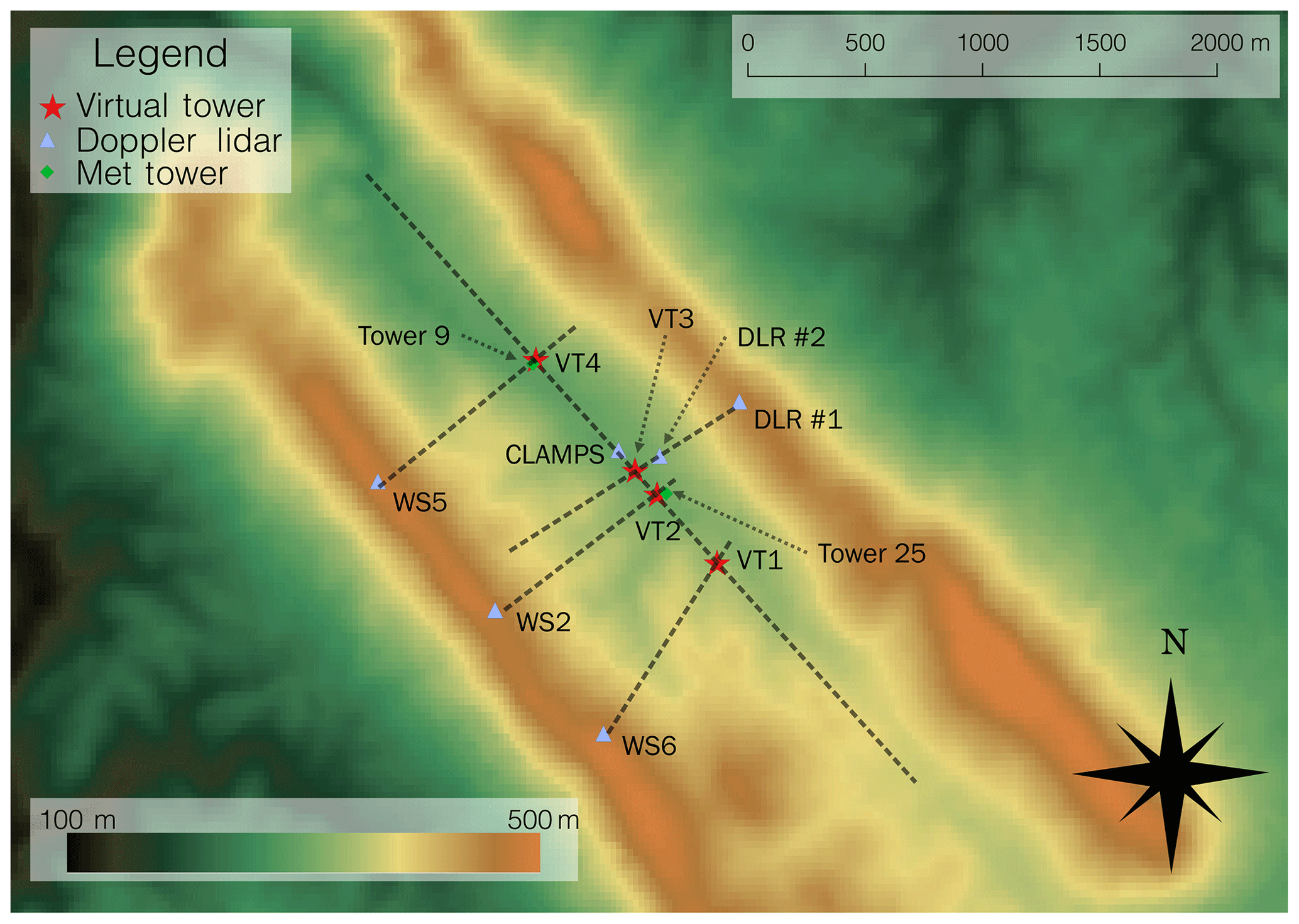
Figure 1Map of DLs, meteorological towers, and virtual towers at the Perdigão site. The color fill corresponds to the height of the terrain above sea level, red stars are virtual-tower locations, blue triangles are DL locations, and green diamonds are instrumented meteorological towers. Tower 9 is a 60 m tower and Tower 25 is a 100 m tower. CLAMPS was located at the Orange Grove site.
The Perdigão experiment is one of the measurement campaigns that took place for NEWA (Mann et al., 2017). Perdigão is a small municipality located in central Portugal that sits adjacent to two parallel ridges of nearly equal height with steep slopes separated by a valley called Vale do Cobrão. The ridge axes extend northwest to southeast and are approximately 1.4 km apart (Fig. 1). Previous wind-tunnel and numerical studies (e.g., Lee et al., 1987; Grubišić and Stiperski, 2009; Rapp and Manhart, 2011) have often focused on the flow over sinusoidal hills. Two parallel ridges are the best approximation in nature to study flow over periodic, sinusoidal type terrain.
Additionally, there is a single 2 MW wind turbine located on the southwest ridge. Wind resources are significantly affected by terrain and land cover. For example, winds at hub height are much higher at the top of a hill than they are on the lee side of the hill. The flow on the lee side of the hill depends largely on the stability conditions, wind speeds, etc. These conditions are important when determining sites where wind turbines will consistently be able to produce energy.
Leading up to the Intense Observation Period (IOP) in the spring of 2017, a meteorological tower had been operating on the SW ridge for a few years. This was used to construct a climatology of the wind directions over the ridge. According to the climatology, winds often were found to be directed perpendicular to the two ridges (Vasiljević et al., 2017). This provided a good opportunity to study the flow in a double-ridge setting. To gather the desired observations, a multinational group of scientists from Europe and the United States converged in Perdigão to measure complex flow at unprecedented spatiotemporal scales. A combination of meteorological towers, DLs, radiometers, and other remote and in situ platforms were dispersed throughout the valley (see Fernando et al., 2019).
2.1 Virtual towers
For this study, multiple different DL configurations were jointly analyzed to retrieve the 3D wind vector in the valley. In total, six DLs from three different institutions were combined to retrieve virtual towers multiple times per hour. Figure 1 shows the location of the DLs considered in this study. Details about the scanning strategies for each DL can be found in Table 1.
Table 1Characteristics of the RHI scans performed by each DL used in this study and the virtual towers they were used for.
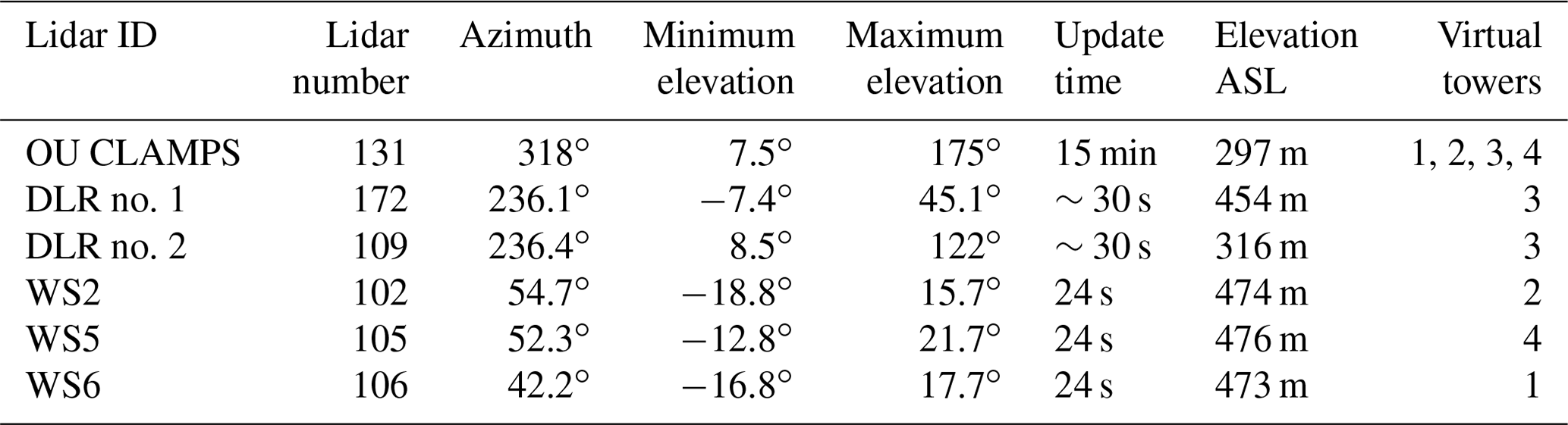
The University of Oklahoma (OU) deployed the Collaborative Lower Atmospheric Mobile Profiling System (CLAMPS, Wagner et al., 2019) at the Orange Grove site, which is located inside the valley and served as central observation hub with a multitude of in situ and profiling instruments during the IOP (see Fig. 5 in Fernando et al., 2019). CLAMPS includes a Halo Photonics scanning DL that performed both cross- (NE to SW) and along-valley (NW to SE) RHI scans every 15 min. In addition, a 70∘ PPI scan was performed every 15 min preceding the RHIs. The remainder of the time, the DL was in stare mode to get vertical-velocity statistics. During Perdigão, the CLAMPS DL was configured such that the first usable range gate was 75 m. CLAMPS also utilizes an Atmospheric Emitted Radiance Interferometer (AERI, Knuteson et al., 2004a, b) and a HATPRO microwave radiometer (Rose et al., 2005) for boundary layer temperature and humidity profiling (Wagner et al., 2019).
The University of Colorado (CU) operated a Leosphere V1 Windcube Profiling DL at the Orange Grove site, colocated with the CLAMPS DL. The CU DL measures the wind speed and direction using the DBS technique (see Rhodes and Lundquist, 2013).
The German Aerospace Center (DLR) contributed three Leosphere Windcube 200S scanning DLs upgraded with the Technical University of Denmark’s (DTU) WindScanner software. Two of these DLs performed continuous RHI scans in the cross-valley direction, which resulted in an RHI approximately every 30 s. One of these DLs was located up on top of the NE ridge (DLR no. 1) and performed RHI scans to the SW, capturing one horizontal component of the wind. The other DL (DLR no. 2) was located on the slope of the NE ridge and performed RHIs to the SW as well.
In addition to the DLR DLs, DTU operated eight DLs of the same kind on top of the ridges. Six of these were configured to do coplanar scans inside the valley so the horizontal wind in the plane and the vertical velocity could be retrieved. These DLs also operated in a continuous scan mode and produced a new RHI every 24 s.
The RHIs from DLR no. 1 and DLR no. 2 overlapped in a coplanar fashion, so by combining these DLs with the CLAMPS DL scans, it is possible to retrieve the three-dimensional wind field in the form of a virtual tower where the three planes intersect. Due to its positioning, DLR no. 2 was able to capture more of the vertical component of the wind in the location of the virtual tower, which allowed the retrieval of the three-dimensional wind vector.
Regarding the DTU DLs, only the DLs from each coplanar cross section that reached deeper into the valley were used. This resulted in three possible 2D horizontal wind retrievals using WS2, WS5, and WS6. The 2D retrievals assume there is no vertical velocity and thus only provide the along- and cross-valley wind components.
In total, four virtual towers distributed along the valley are retrieved every 15 min when the CLAMPS DL performed its along-valley RHI. The virtual towers typically cover heights from 50 to 600 m above the valley floor depending on the minimum and maximum height of RHI intersection. It should be noted that different to previous virtual-tower retrievals (Calhoun et al., 2006; Hill et al., 2010; Damian et al., 2014; Pauscher et al., 2016; Debnath et al., 2017) the DL data used in our study were not collected using coordinated scans that were specifically programmed for 2D and 3D wind retrievals. Instead, our objective was to test the quality of virtual-tower retrievals in complex flows using data from uncoordinated scans with overlapping sampling volumes.
When combining data from the uncoordinated DL scans in the virtual-tower retrievals, several analysis steps were necessary. First, data from each DL were converted to a common coordinate system. Once the X–Y location of the RHI intersection (i.e., the virtual tower) was determined, minimum and maximum heights were manually determined for each of the virtual towers. A vertical spacing of 10 m was selected for the virtual towers to ensure that we had unique DL range gates to derive the 3D/2D winds for each height. Using the location of these points, the azimuth () and elevation (), relative to each DL, were calculated and used to linearly interpolate the radial velocity from each DL to a new radial velocity at the point of the tower (). We evaluated the difference of cubic spline interpolation to linear interpolation and found that differences of less than 0.1 m s−1 occur, which is well within the uncertainty we set for the DL radial wind speed measurement. Since neither cubic spline nor linear interpolation can be assumed to be a true representation of the atmospheric flow field, we decided to apply the simpler, computationally more efficient method of linear interpolation. From there, retrieving the 3D/2D wind vector is as simple as solving the 3D transformation matrix for the radial velocity vector to get
where u is the velocity in the east–west direction, v is the velocity in the north–south direction, w is the vertical velocity, Vri is the interpolated radial velocity from the DL, ϕi represents the elevation, and θi represents the azimuth angles.
Temporal resolution of the virtual towers is limited to the time resolution of the CLAMPS RHI. Since the scans were not coordinated to sample the same volume of space simultaneously, a time window needed to be determined. Choukulkar et al. (2017) used a time window of 15 s when comparing uncoordinated multi-Doppler retrievals to a sonic anemometer and found reasonable agreement. For this study, all the time periods considered took place overnight, which generally had more steady flow due to the lack of turbulent mixing. Therefore, a time window of 60 s is used. While most of the data fell within this window, there are time periods late in the IOP where retrievals are not possible due to the CLAMPS RHI starting too late to be captured in the 60 s window.
3.1 Uncertainty analysis
Possible uncertainties contained in the retrieval are analyzed using an idealized scheme derived from the methods discussed in Hill et al. (2010):
where is the possible random error associated with each DL line-of-sight wind speed measurement, ui is the Cartesian velocity component of the wind, and rj is the radial velocity vector for each DL. This results in a formula for the error for each velocity component given a combination of the various azimuths, elevations, and ranges for each lidar. For this study, it is assumed that is 0.2 m s−1 based on prior experience with the systems used (Kigle, 2017; Wildmann et al., 2018a). Using a coordinate system that was aligned with the valley of the Perdigão site and choosing parameters representative of the scan configurations of the various DLs used, we computed the uncertainty of the retrieved along-valley, across-valley, and vertical-velocity components (Fig. 2). The results clearly show that with increasing height, as the DL beams point increasingly vertical, uncertainties in the horizontal wind components get larger and uncertainties in the vertical velocity get smaller. It can further be noted that the errors in the horizontal wind components in the cross-valley direction are much larger in the 3D retrieval. This is due to the proximity of VT3 to the CLAMPS DL; gates at much higher elevation angles must be used, meaning less of the horizontal component of the wind in the along-valley direction is contained in the measured radial velocities.
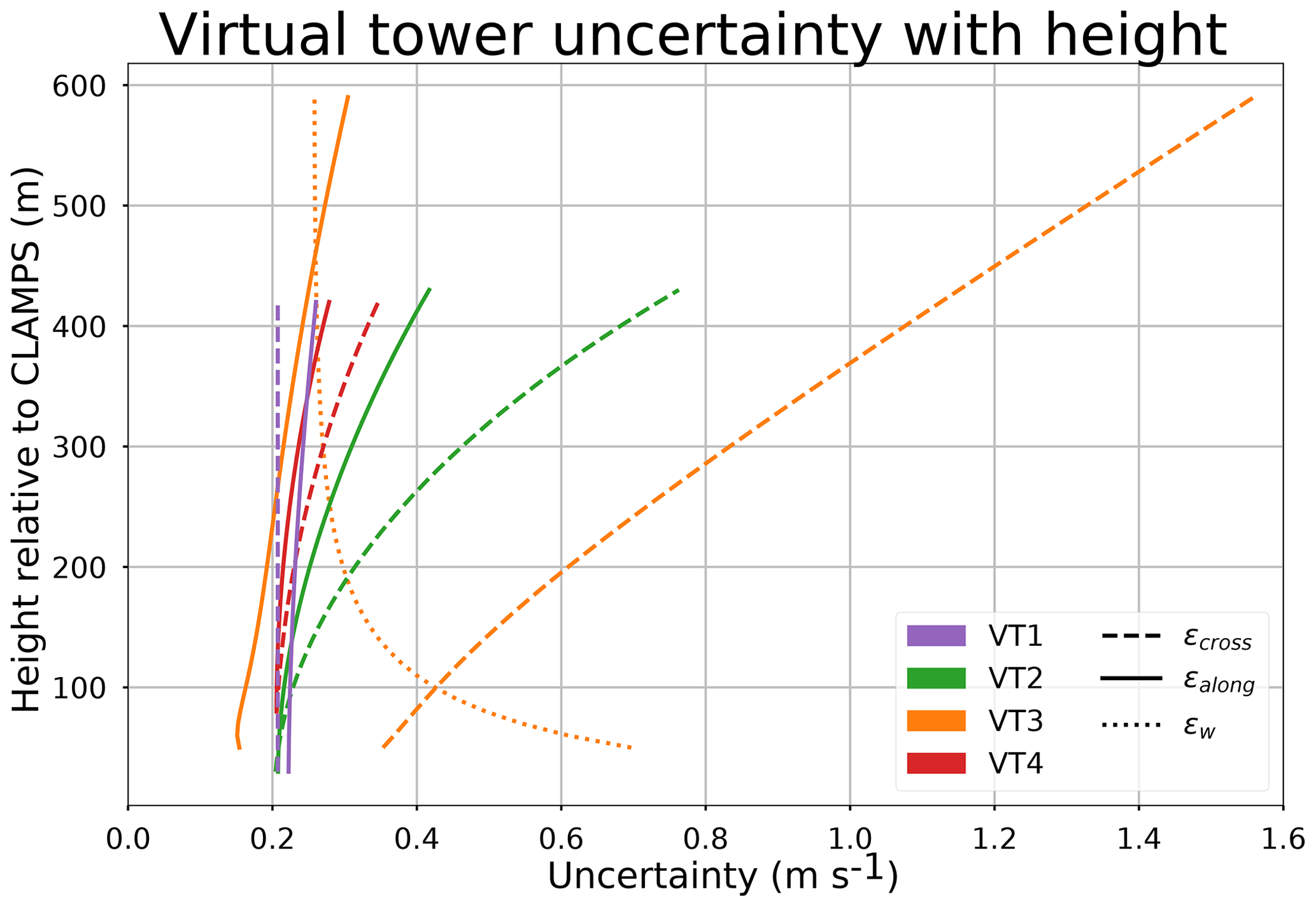
Figure 2Uncertainty from the various virtual towers. Solid lines are uncertainty in along-valley direction, dashed lines are uncertainty in the cross-valley direction, and dotted lines are uncertainty in w. The color corresponds to the virtual tower (see Fig. 1). Note that most of the uncertainty is contained in the along-valley direction since the CLAMPS DL was scanning at a high elevation angle (elevations used ranged from 21 to 77∘). Additionally, the further away the virtual tower was from CLAMPS (i.e., the lower the elevation angle had to be), the lower the uncertainty.
3.2 Impact of terrain on 2D towers
Since we had only one site where all three components of the wind vector could be retrieved but had multiple 2D virtual-tower sites where the horizontal wind vectors were retrieved assuming that the vertical wind velocity is negligible, it is important to quantify the errors introduced in the 2D retrievals. This is particularly important in complex terrain where large vertical velocities are often present. To do this, a theoretical idealized setup was constructed (Fig. 3). DL1 and DL2 are fixed in place, but DL3 is allowed to move in range away from the tower, thereby decreasing the elevation angle required to observe the same point. This setup is meant to mimic the DL placements for the 3D tower (see VT3 in Fig. 1). For assessing the errors introduced by neglecting the vertical wind velocity in the 2D virtual towers only DL1 and DL3 are then used for wind retrievals.
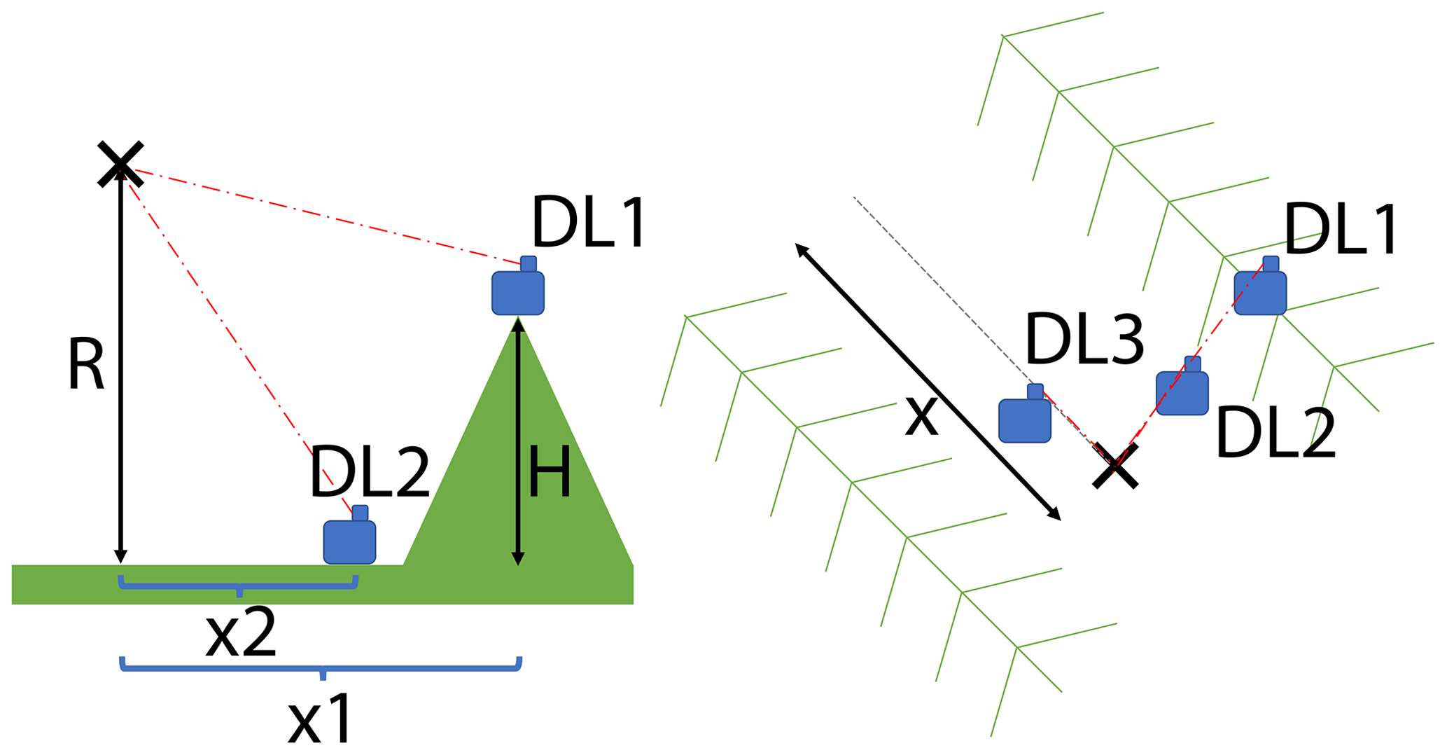
Figure 3Idealized setup to examine the errors associated with neglecting the vertical velocity and only producing 2D virtual towers. The setup is meant to closely mimic the positions of the CLAMPS DL, DLR no. 1, and DLR no. 2 used in the 3D virtual tower. DL3 is varied along x to simulate different elevation angles.
Next, we selected different 3D wind speeds and directions at the intersection of all the DL beams and calculated the radial velocities that are observed by each DL by rearranging Eq. (1). By only using the radial velocities from DL3 and DL1, a 2D retrieval similar to the 2D retrievals done for the real virtual towers can be simulated (with one DL on top of the ridge and with the CLAMPS system inside the valley). However, for fully 3D flow fields, the assumptions used for the 2D towers retrievals are violated and contributions of the vertical motions to the radial velocities will be falsely projected into horizontal motions causing errors in the along- and across-valley wind components. Multiple vertical velocities were selected that mimic the range of the observed vertical stare data collected with the CLAMPS DL throughout the IOP, which allows us to get quasi-realistic assessments of the errors inherent in the 2D virtual-tower retrievals.
Figure 4 shows expected errors in horizontal wind speed and direction that arise if the vertical component of the wind is assumed to be zero. The dashed vertical lines shown in Fig. 4 indicate the errors that can be expected for the various virtual towers at the Perdigão site given the location of the different DLs employed in the retrievals. It becomes immediately apparent that not accounting for vertical velocities can introduce large errors in wind direction estimation at ridge height. Vertical velocities as large as 2 m s−1 were often observed in the CLAMPS DL vertical stares, which can cause errors in wind direction estimation to be near 40∘ if the retrievals only use two DLs. Due to the close proximity to CLAMPS, VT3 would have been the most erroneous 2D retrieval. However, it was possible to retrieve the 3D winds from this location.
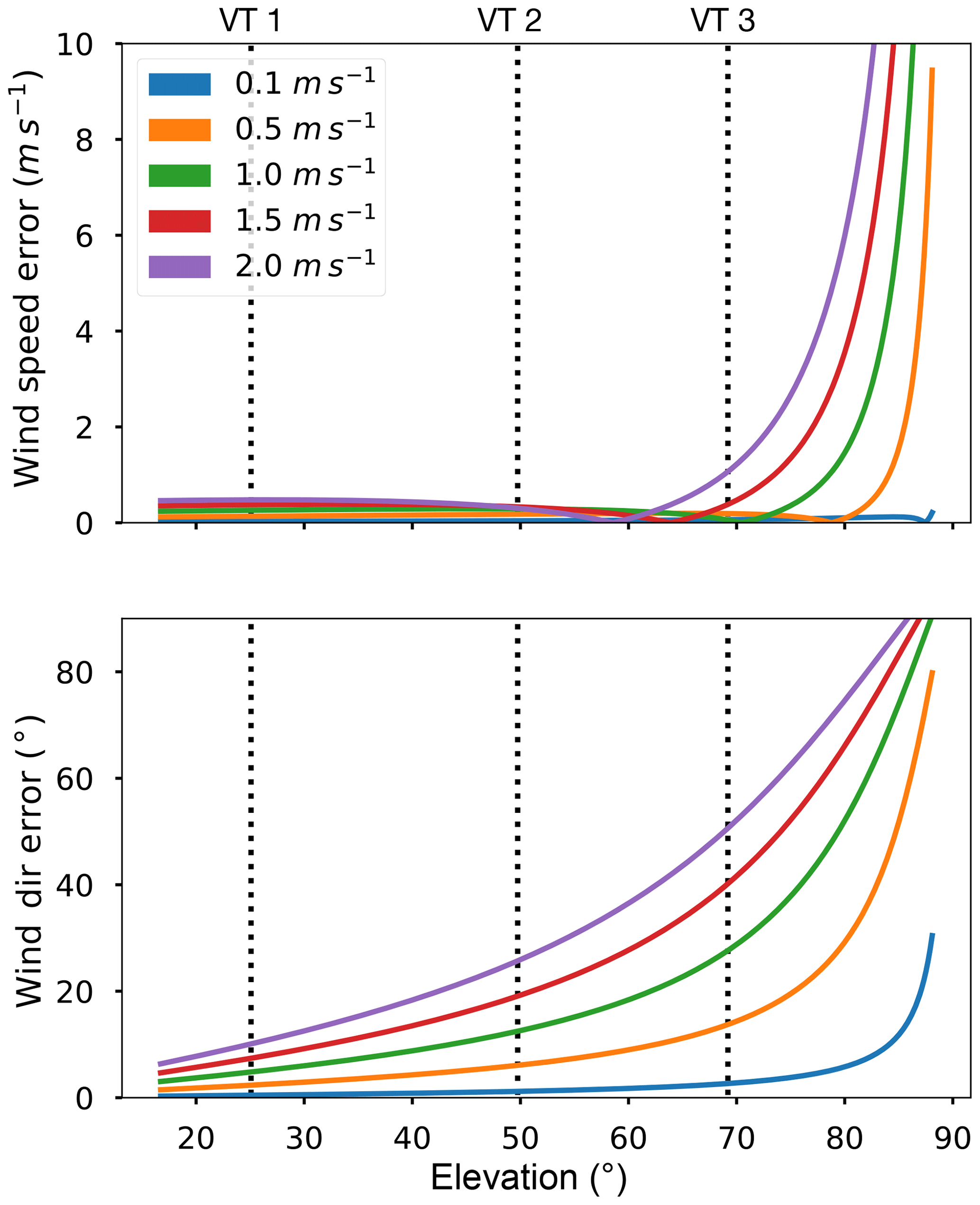
Figure 4Wind speed and direction errors associated with neglecting the vertical velocity in 2D virtual towers. Results are for R=300 m and H=200 as depicted in Fig. 3. These values were chosen to mimic virtual-tower measurements slightly above ridge height. The line colors correspond to different vertical velocities examined. The vertical lines correspond to the elevation for VT1, VT2, and VT3 for the given R and H; thus these are the expected error for this point in space for these VTs. Note that as vertical velocity increases, error in wind direction estimation increases even at relatively low elevation angles.
4.1 Selected case studies
As mentioned in Sect. 1, one of the challenges of our study was the fact that none of the datasets available was free of limitations and all DL retrieval methods applied introduced measurement errors. In addition to the systematic uncertainty analyses presented in the previous section, we decided to illustrate the strengths and weakness of the different retrieval methods by selecting cases from the Perdigão IOP with flow patterns of increasing complexity. Given the topography of the site, we assumed that the flow can be considered quasi-2D for wind directions perpendicular to the valley; i.e., under such conditions the flow variability along the valley is expected to be small. Note that there can still be a component of the wind directed in the along-valley direction; the distinction is that this component does not vary along the length of the valley contained inside the study domain (i.e., between WS5 and WS6). To ensure the flow was quasi-2D, the along-valley RHI scans from the CLAMPS DL were visually inspected to ensure any along-valley component of the wind did not vary in the study domain.
We focused the analysis on three cases: first we selected a case with quasi-2D flow and small vertical velocities, next we chose a quasi-2D flow case with large vertical velocities, and last we selected a fully 3D case with complex flow interactions that are associated with strong variability of the flow along the valley. The selected days from the Perdigão IOP were subjectively identified based on the analysis of DL scans and stability profiles. Additionally, data availability was taken into account.
For the first case, we would expect that the VTs and single-Doppler retrievals agree well, even though the sites vary along the valley. We argue that in this case, the observed differences between the retrieval methods are primarily caused by measurement errors and uncertainties in the retrieval methods and less by flow variability; i.e., the comparison allows us to assess the measurement errors introduced by different retrieval approaches. The second case, with stronger vertical motions while still being quasi-2D, allowed us to analyze the amount of error vertical motion introduces into the 2D retrievals for a realistic scenario. The observed differences can then also be compared with the results from the systematic study described in Sect. 3.2 for cross-validation. Once the virtual-tower uncertainties are well characterized, it is then possible to illustrate how the virtual towers can be used to understand flow phenomena for a highly complex case.
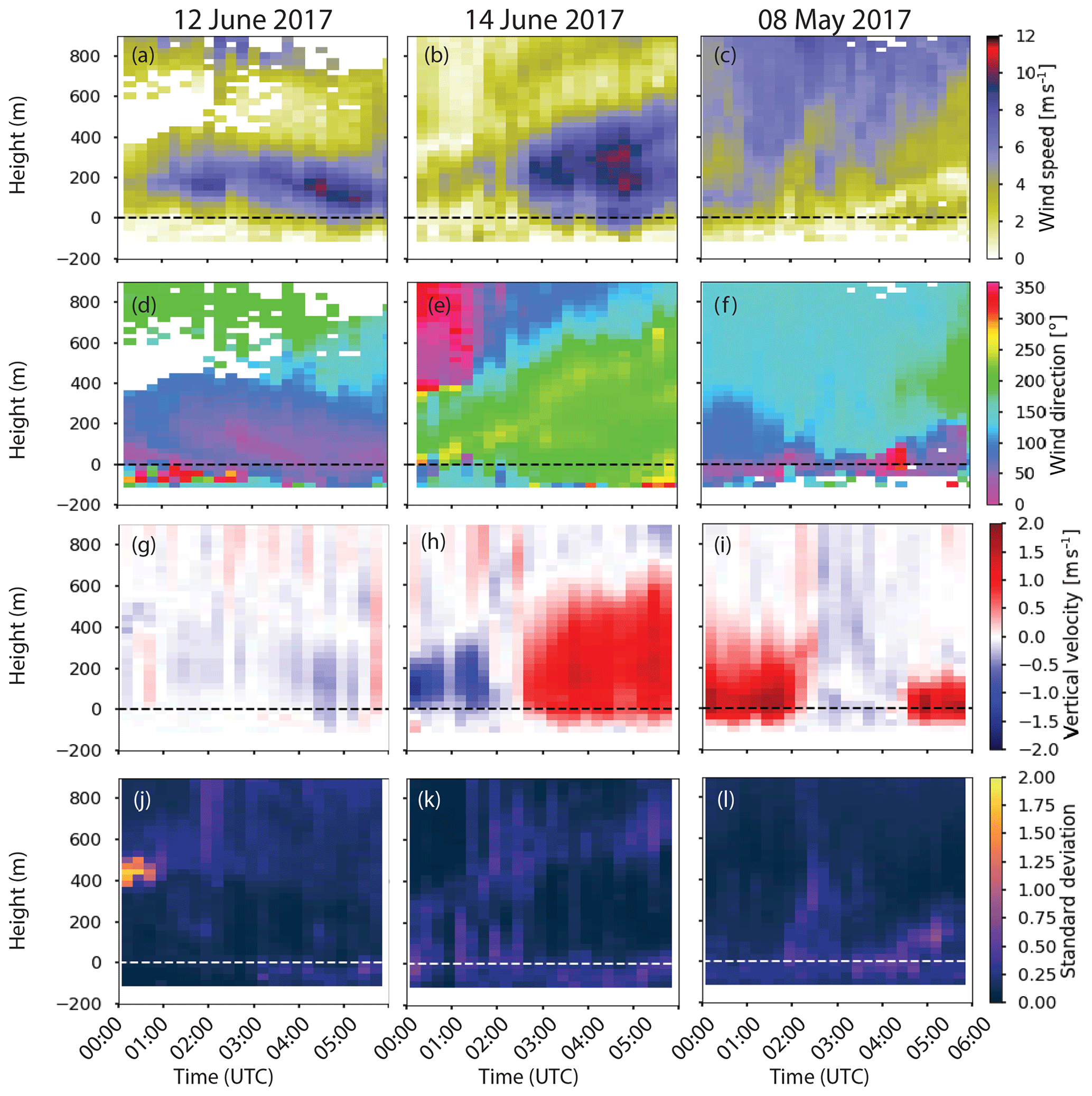
Figure 5Time–height plots of three nights observed by the CLAMPS system. The top row (a–c) shows wind speed derived from the 70∘ VAD scan, the second row (d–f) shows the wind directions from the VAD, the third row (g–i) shows 15 min averages of vertical velocity derived from the CLAMPS vertical stare data, and the bottom row (j–l) shows the standard deviation from the averages. The left column shows data from 8 May 2017, the middle column data from 12 June 2017, and the right column data from 14 June 2017. The height axis is relative to the base of the wind turbine on the southwest ridge, which is a proxy for ridge height.
4.1.1 Quasi-2D flow with limited vertical motion
For our simplest case, we selected a day with wind speeds that exceeded 7–10 m s−1 at or above ridge height with wind directions perpendicular to the ridge axis. This minimizes the spatial variability of the flow along the length of the valley. Additionally, we target a time period during which the observed vertical velocities were largely less than 0.5 m s−1 by examining the vertical stare from the CLAMPS DL – 12 June 2017 from 00:00 to 06:00 UTC fit these criteria.
During this period, a shortwave trough was off the coast of Portugal. Winds at 500 mbar were approximately 10 m s−1 from the SW. No discernible mesoscale surface features were present as a result of the trough. However, there are a number of mesoscale circulations that dominate the flow around Perdigão (Fernando et al., 2019). Thermal flows from the Serra da Estrela to the north often compete against synoptic-scale flows. This can introduce unique layering of wind speeds and direction near the ground. Winds during this period were 5–10 m s−1 throughout the night (Fig. 5a) and were out of the northeast (Fig. 5d). A strong temperature inversion was present in the valley. Additionally, there was very little vertical motion and turbulence (Fig. 5g and j).
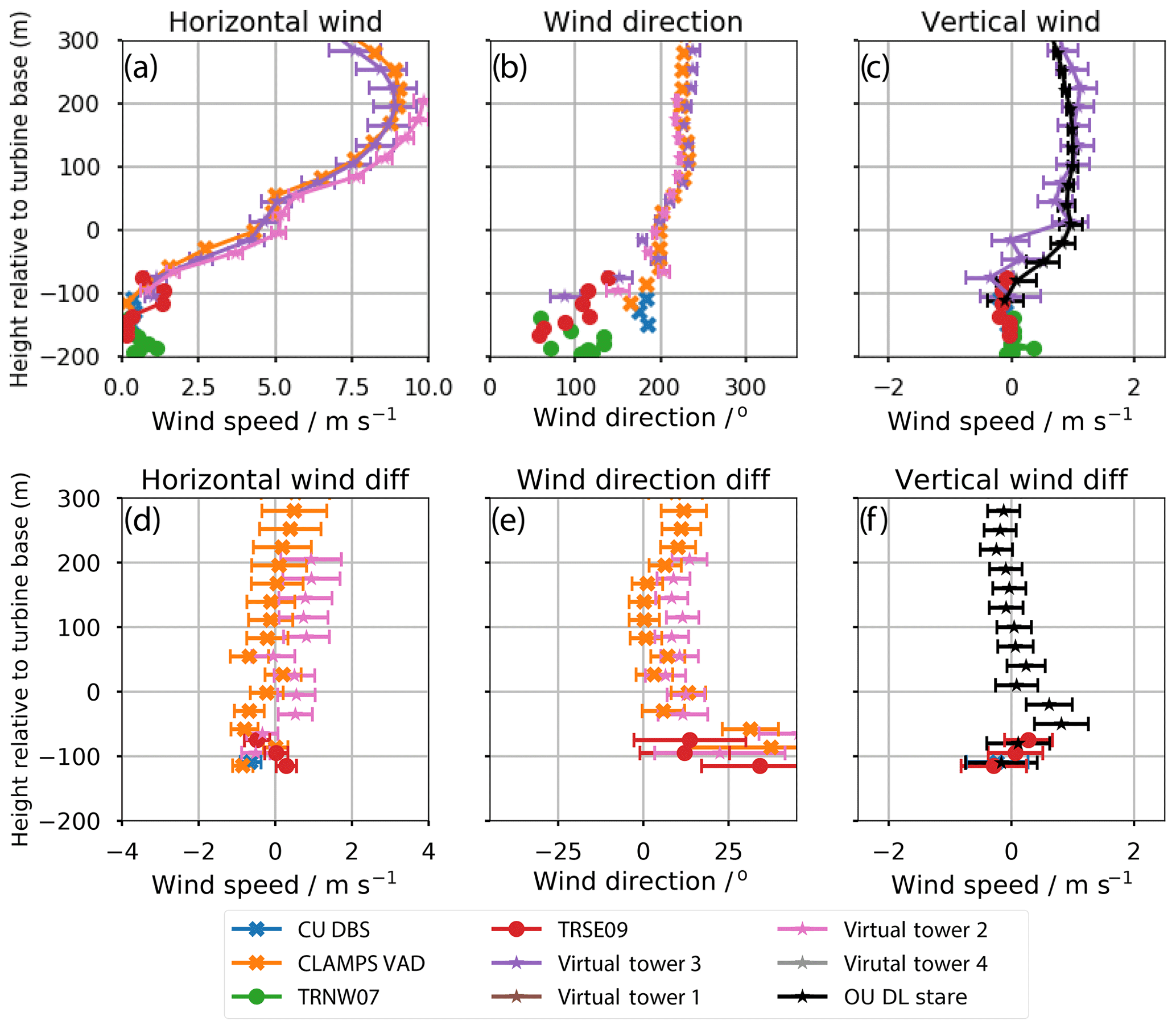
By starting with a relatively simple case, it is possible to directly compare the retrieval methods with minimal violations to the underlying assumptions. Unfortunately, VT4 and VT1 did not meet the retrieval criteria because the CLAMPS DL became slightly out of sync with WS5 and WS6, and the time difference between scans did not meet the retrieval criteria. However, for this application, having VT2 and VT3 will suffice since they are the closest to each other spatially (Fig. 1). Differences between all the various systems compared to VT3 are shown in Fig. 6 with the various uncertainties propagated through the difference. The CLAMPS vertical stare indicates that VT3 is overestimating the vertical velocity by approximately 0.5 m s−1 from −40 to 180 m (Fig. 6c and f). In this layer, there are biases in the VT3 wind speed and direction as well (Fig. 6d and e) while the other instruments fall within their respective levels of uncertainty. The wind speed of VT3 is biased by approximately 10∘ while the wind speed is biased by approximately 0.5 m s−1. Where the VT3 vertical velocities agree with the CLAMPS vertical velocities above 180 m, the wind speeds and direction are within the degree of uncertainty in the retrievals.
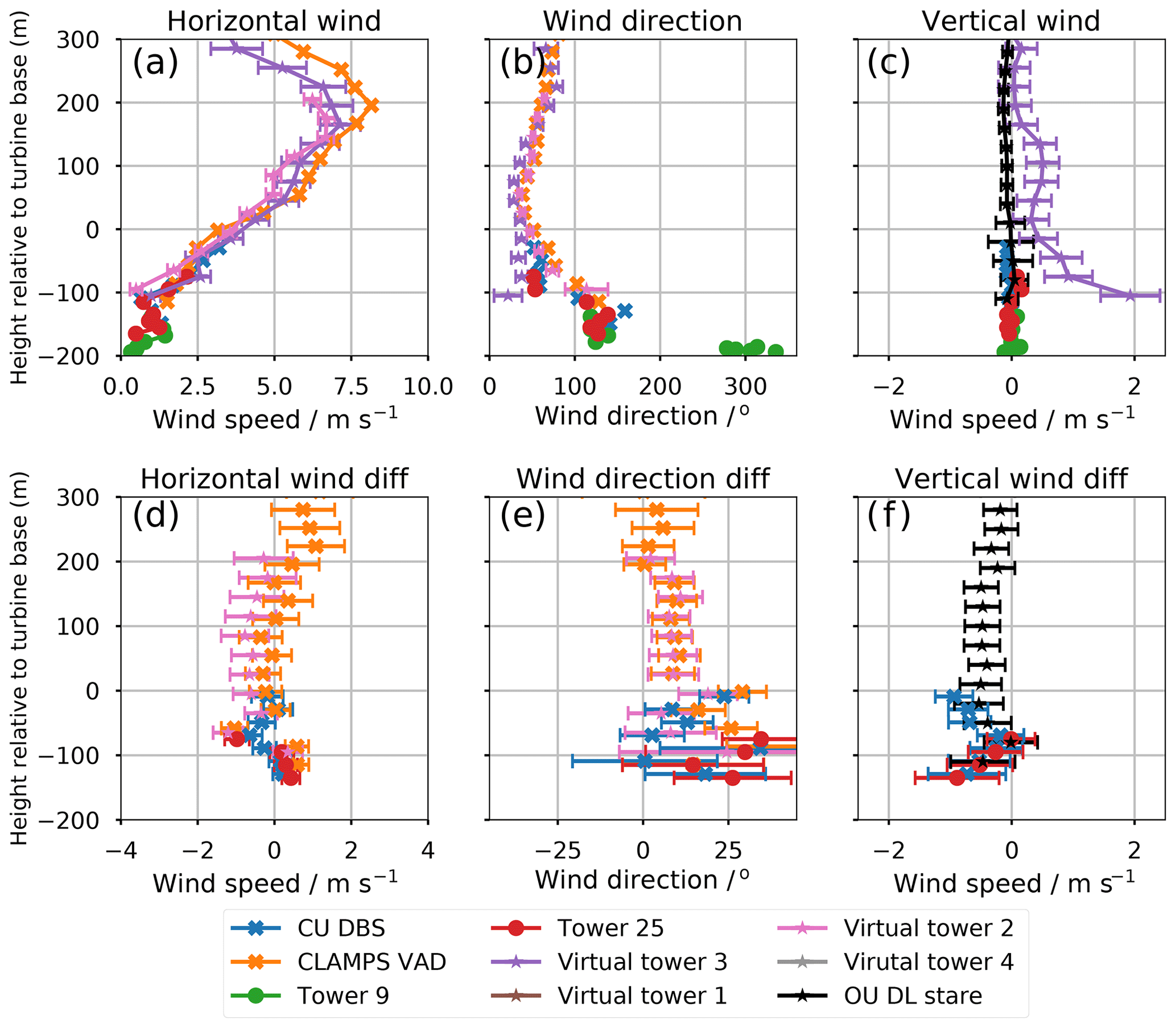
Figure 6Profiles of horizontal wind speed (a), wind direction (b), and vertical velocity (c) of the CU DBS (blue), CLAMPS VAD (orange), VT2 (pink, 2D), VT3 (purple, 3D), Tower 25 (red), and Tower 9 (green) from 12 June 2017 at 02:55 UTC (discussed in Sect. 4.1.1). Additionally, profiles of the difference relative to VT3 are shown (d–f). VT4 and VT1 are not available for this time period due to DL malfunction and not meeting retrieval criteria, respectively. Note the height axis is relative to the base of the wind turbine, which is a proxy for the height of the ridge. Additionally, the error bars on the CLAMPS DL stare profile (f) are the standard deviation of the vertical velocities observed between 1 min before and 1 min after the virtual-tower time. Uncertainty is propagated through the difference, hence the appearance of error bars on Tower 9, Tower 25, and the CLAMPS VAD in (d–f).
4.1.2 Quasi-2D flow with strong vertical motion
Similar to the previous case, we again targeted a time period with wind speeds that exceeded 7–10 m s−1 at or above ridge height and wind directions that are perpendicular to the ridge axes, during which the flow along the ridges can be assumed to be more quasi-2D. As with the previous case, RHIs from all the DLs were inspected to ensure this was the case. However, this time we selected a time period with relatively strong vertical motions greater than 1 m s−1. This allowed instantaneous double- and triple-Doppler virtual-tower measurements to be contrasted to single-Doppler measurements (such as VADs). Additionally, the error analysis from Sect. 3.2 could be validated using the 3D tower. During the overnight hours of 14 June 2017, the shortwave trough mentioned in Sect. 4.1.1 had moved over the area. The valley was neutrally stratified through the night. Winds after 03:00 UTC increased to approximately 10 m s−1 from the southwest (Fig. 5b and e), and a persistent wave formed, causing large and steady vertical velocities over the CLAMPS site (Fig. 5h and k).
For this case, consistent differences between the 2D and 3D retrievals can be noted where there are vertical velocities present in the profile. Based on Fig. 4, one would expect there to be approximately a 10 to 20∘ difference in wind direction between the fully resolved 3D tower (VT3) and the 2D tower (VT2) at 100 m above ridge height, where the vertical velocity was approximately 1 m s−1 (Figs. 5h and 8c). Figure 8e shows that the wind direction from VT2 differs by 10 to 15∘ from the wind direction at the CLAMPS VAD and VT3, which lends credence to the previously discussed idealized model and provides a simple way to estimate the uncertainty in the 2D towers due to the vertical motion. There are also slight differences in wind speed present. While VT3 and the CLAMPS VAD agree within the range of uncertainty at ridge height and above, VT2 is consistently indicating 1 m s−1 higher wind speeds (Fig. 8a and d), which agrees well with the expected offset in Fig. 4. Again, the time series of VT3 and VT2 fall within the range of wind speeds observed by the tower, even capturing the wind speed increase that occurred around 04:00 UTC (Fig. 7c and f).
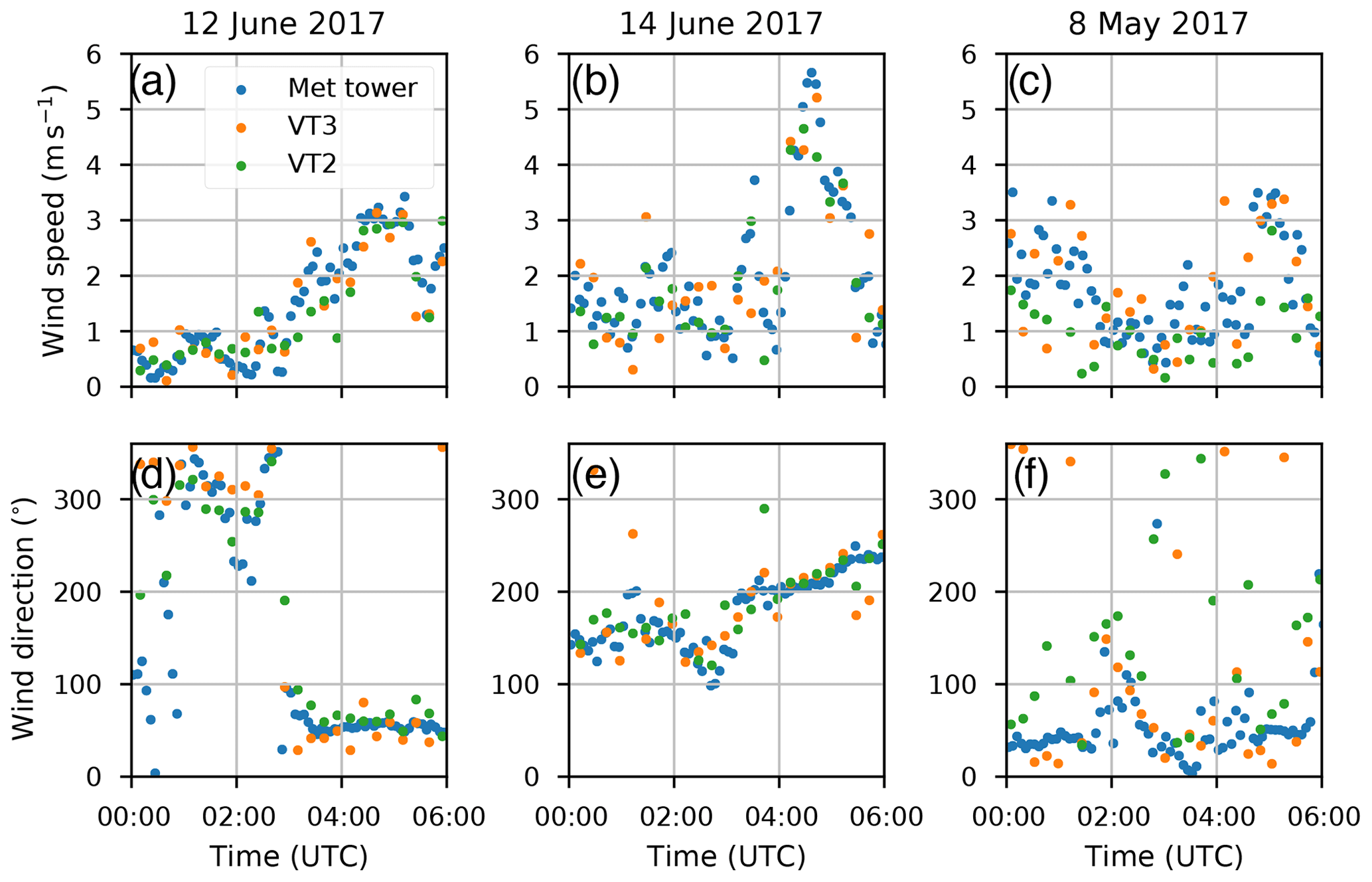
Figure 7Time series of wind speeds (a–c) and wind directions (d–f) from VT3 (orange points), VT2 (green points), and the 5 min averaged data from Tower 25 (blue points) at 100 m for the three selected cases.
4.1.3 Spatially complex case
While the two previous cases were selected with the intent of assessing the retrieval methods by limiting the analysis to quasi-2D flows, the final case was chosen to illustrate how useful the virtual towers can be for measuring the spatial variability of features along the valley. A moderately complex case, 8 May 2017, was selected. During this time, there was a low-pressure system off the coast of the Iberian Peninsula and a ridge over Perdigão. Aloft, winds over the IOP site were from the southwest at 15 m s−1 around 500 mbar.
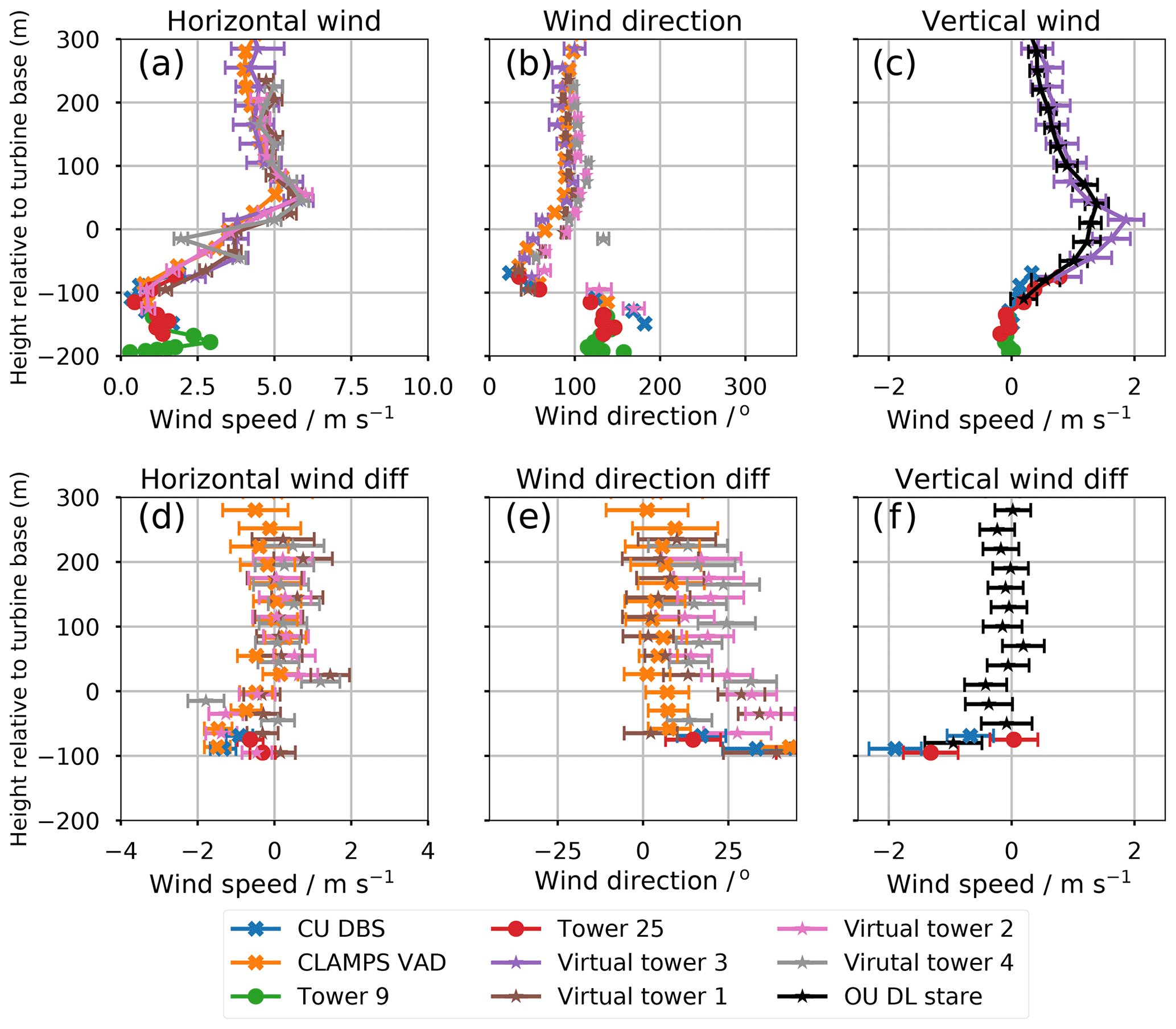
Figure 9Similar to Fig. 6, only with VT1 (brown) and VT4 (gray) included. Profiles are from 8 May at 00:32 UTC. In general, the methods agree well above the ridge (generally greater than 100 m), but results begin to get noisy 100 m below ridge height. For the sake of readability, only every third point has been plotted for the virtual towers.
The complexity of the flow for 7–8 May is shown in Fig. 5. Generally, winds are from the northeast during the night of 7 May. On 8 May, winds veered through the night and were less than 3 m s−1 at ridge height (Fig. 5c and f). Wind directions vary widely since the mean wind is interacting with various slope flows occurring inside the valley. Numerous periods of strong vertical motion were observed over the CLAMPS site due to waves forming as a result of the terrain. On 8 May, a unique, double-wave feature was observed along with a recirculation within the valley. This occurred during the period of relatively low wind speeds around 05:00 UTC (Fig. 5c). The double-wave feature did not appear often during the rest of the IOP and lends itself well as a good test for the virtual-tower retrievals, especially the 3D virtual tower, given its complex evolution over time and space.
As mentioned previously, the traditional DL technique for retrieving the wind speed and direction with a single DL is the VAD or the DBS technique. However, in the overnight hours of the Perdigão campaign, the assumption of horizontal homogeneity is often violated due to flow phenomena created by the terrain. This is expected to be particularly prominent at the lowest levels of the VAD or DBS profiles near the surface. We will now examine data from 8 May (Sect. 4.1.3) to assess the virtual towers in weak, highly variable flow. Using the spatially distributed virtual towers can be helpful to study these type of flows.
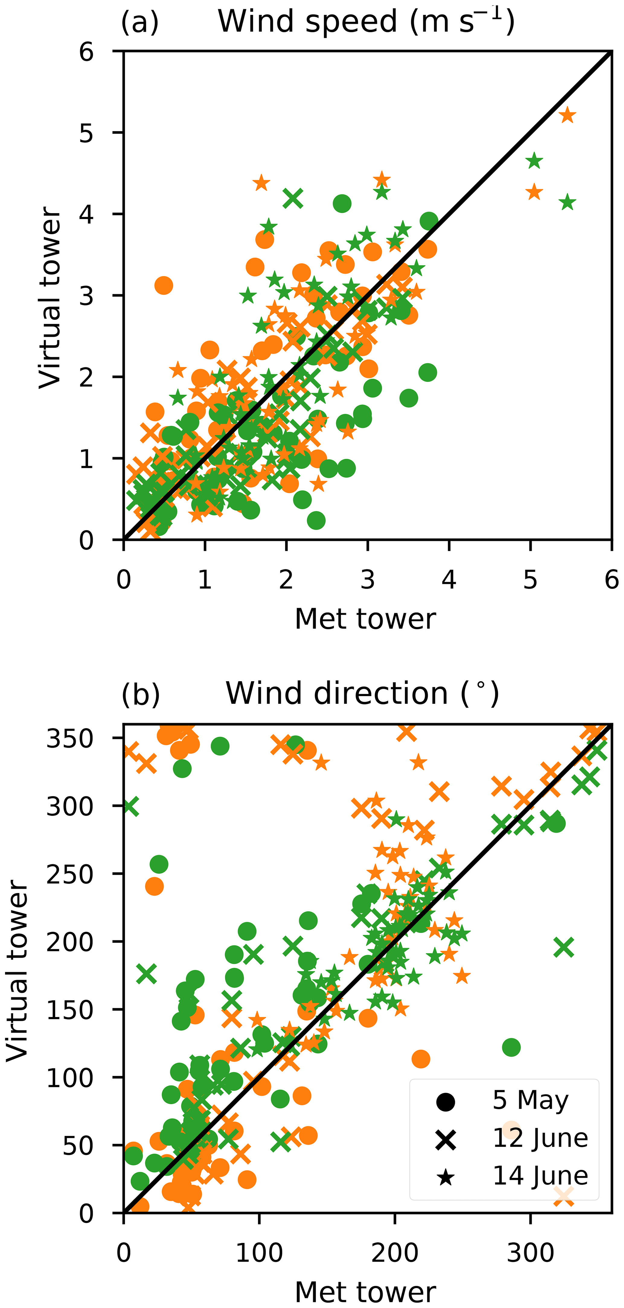
Figure 10Scatter plots of the wind speeds (a) and direction (b) from VT2 (green) and VT3 (orange) vs. the 5 min averages of wind speed and direction from Tower 25.
Figure 9 illustrates how single DL retrievals can break down in complex terrain. A few things become apparent from the comparison. In general, the CLAMPS VAD falls within the uncertainty of the VTs in wind speed and direction greater than 100 m above the ridge. Looking closer at VT retrievals above ridge height, there seems to be a consistent offset in wind direction between VT3 and each of the other 2D towers (Fig. 9e), which can be explained by the vertical velocities, as discussed in the previous section. This offset gets larger as the profile approaches ridge height, where the vertical velocities are larger.
Around 100 m below ridge height, the different techniques start to diverge. Wind speeds stay relatively consistent between each technique below ridge height, but the directions are highly variable. In particular, the wind directions from the CU DBS scan differ greatly from VT3. The CLAMPS VAD tends to agree slightly more but still significantly differs from the collocated VT3 just below ridge height.
The vertical velocities from VT3 and the CLAMPS DL vertical stare also agree within the uncertainty VT3 above ridge height. Around the same level as the wind speeds and directions, the stare and the 3D virtual tower start to diverge. The differences could be due to each measurement representing a different time. The tower data are 5 min averages, while the CLAMPS DL stare data and the CLAMPS/DLR virtual tower are instantaneous measurements at slightly different locations, so some differences are to be expected.
Breakdowns in the single-Doppler DL retrievals can be observed by closely examining Figs. 6 and 8, assuming VT3 is taken to be the most accurate representation of the wind speed and direction. Similar to the highly complex case, there is relatively good agreement well above ridge height, where the flow is less affected by the terrain. Inside the valley however, the flow is less horizontally homogeneous due to the complexity of the valley floor. This causes there to be differences between the virtual towers and the single-Doppler retrievals (for example, below −100 m in Fig. 8).
In summary, Fig. 9 shows how all the towers (both virtual and real) compare to one other. In general, the wind speeds all line up nicely. There are differences in the wind direction though. The differences can likely be attributed to the error associated with the 3D towers discussed in Sects. 3.2 and 4.1, though they could also be due to the complex flow field as well. As vertical velocities become larger at and slightly below ridge height, the spread in wind direction gets slightly larger. Additionally, the spread is approximately what would be expected from Fig. 4. However, there is still noticeable spread in the lowest levels that is likely due to heterogeneity of the terrain. Additionally, Fig. 7 shows that VT3 agrees well throughout the night; however, VT2 contains a larger spread in wind directions. To determine if these are real, the flow needs to be examined in a spatial sense. Taking into consideration all the sources of uncertainty in the towers, it is possible to examine the flow in and around the valley at a high level of detail. Overall, the virtual towers perform reasonably well during each case study (Fig. 10). A slight positive bias in wind direction was present in VT2 since it suffers from the errors described in previous sections.
4.2 Spatial analysis
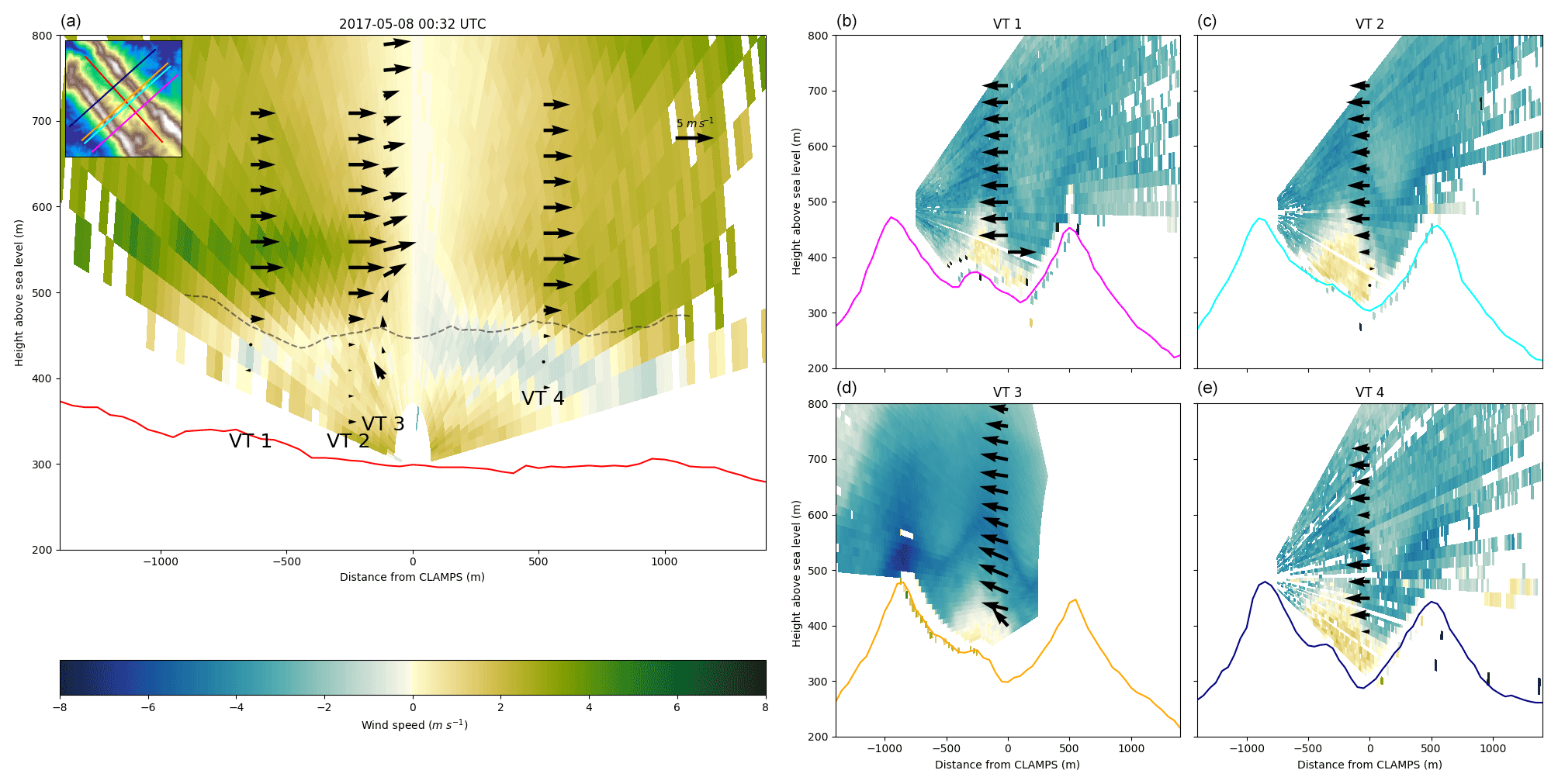
Figure 11(a) Along-valley cross section of the flow for 8 May at 00:32 UTC. The color fill is the radial velocity projected into the horizontal from the CLAMPS RHI used to create the virtual towers. Positive values indicate flow in the +X direction, which is directed to the NW. The overlaid vectors are the components of the virtual towers projected into the plane of the RHI scan, the inset plot shows how the terrain cross sections are oriented and where they are located, and the dashed gray line is the height of the SW ridge. (b–e) Similar to the along-valley plot on the left, only in the cross-valley sense. +X here points to the NE. The color of the line matches the cross section indicated in the terrain inset. This plot corresponds to the profiles shown in Fig. 9.
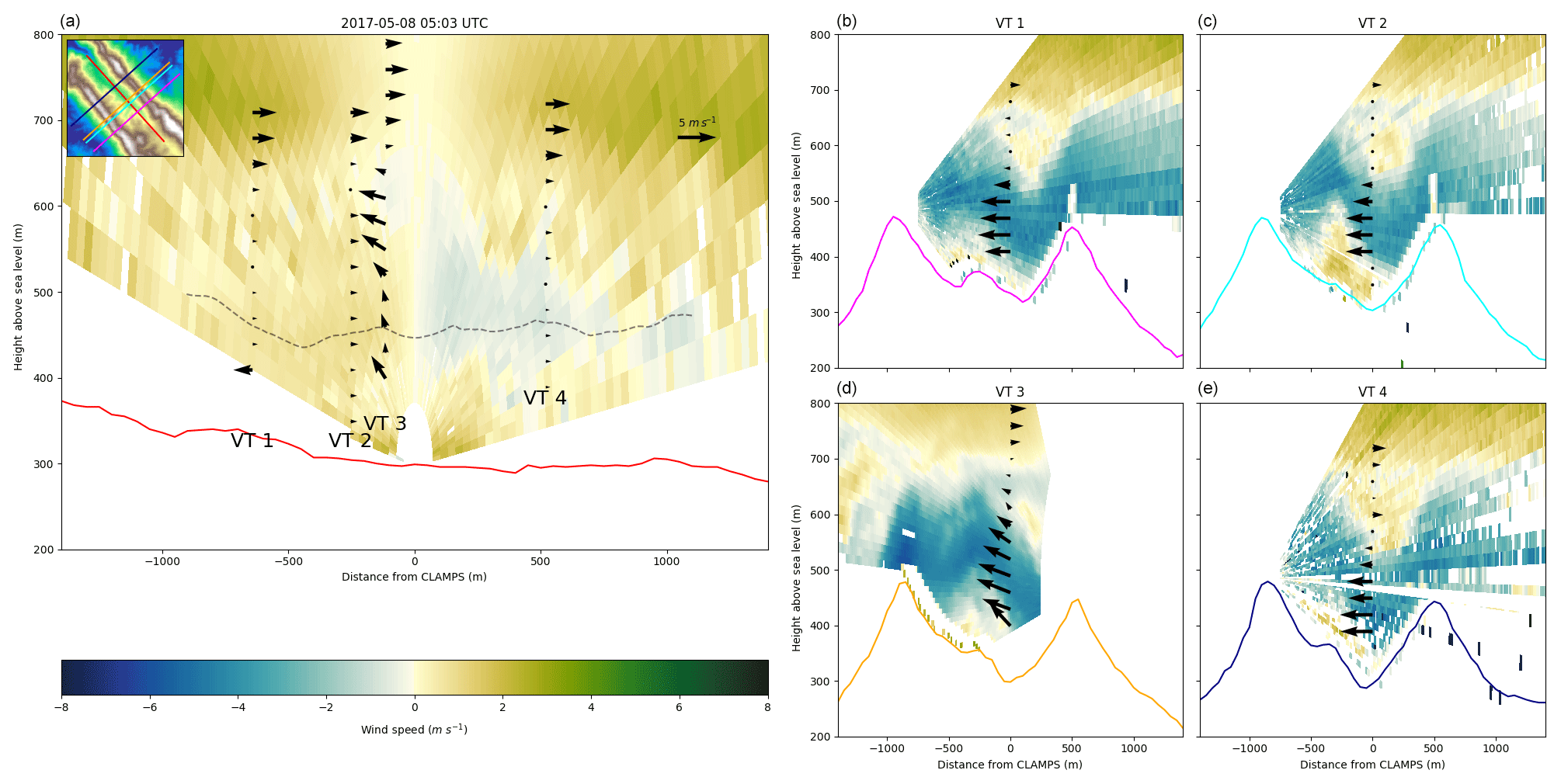
Figure 12Same as Fig. 11 but for 05:03 UTC. Note the different structure of the wave and the shear layers in the cross-valley winds. Also note the different strengths of the recirculations.
One of the main reasons Vale do Cobrão was chosen for the experiment was the quasi-two-dimensional nature of the ridges; they were thought to be the best way to represents a series of periodic rolling hills and that flow perpendicular to the ridges could also be considered quasi-2D. While this assumption is valid during some nights with higher wind speeds, periods with lower wind speeds tend to have more spatial heterogeneity. In order to visualize this heterogeneity, it is best to think of wind components in the cross-valley and along-valley sense.
Analysis of the virtual towers coupled with the cross-valley RHIs from the DLR and DTU DLs often shows that the flow can not be considered entirely 2D, especially at lower wind speeds. In Fig. 11, cross-valley flow is approximately −4 m s−1. No clear jet is present in the RHI or virtual towers, but there is a large recirculation in the valley. During this time period, flow was strong enough that the circulation was present in all the cross sections of the valley. However, the size and strength of the recirculation varied due to the topography of the valley floor. Where the recirculation is strongest, cross-valley wind speeds are slightly reduced in the virtual tower (VT2 and VT4). This is especially prominent in the lowest levels of the virtual towers near the circulation. This also appears in some of the levels well above the valley, which is significant because it implies that the recirculation is correlated with changes in the flow well away from the feature itself. This recirculation could be a rotor or hydraulic jump type feature as observed in Neiman et al. (1988).
Looking at the along-valley component of the flow, winds are very calm and near zero within the valley. There does appear to be a weak jet just above the ridge at 550 m. There is evidence of a wind speed maximum near the surface, which indicates there is a downslope flow. This feature was often observed overnight in the along-valley RHI from CLAMPS. Though the virtual towers do not extend far enough into the valley to capture this flow, the meteorological towers are able to capture the near-surface speed maximum associated with it (Fig. 9). This persistent flow adds to the three-dimensionality of the flows present in the valley.
Analysis of a different time period during the night of 8 May further shows the complexity of the flows in the terrain. During this night, winds veered rather quickly aloft and weakened closer to the surface (Fig. 5). An interesting transition occurs and a unique double wave forms within the valley along with a shear layer (Fig. 12). Like the previous case, there is little along-valley component of the wind below the ridge. There is still a speed maximum in the down-valley flow in the lowest 20–30 m of the CLAMPS RHI scan, which is indicative of the aforementioned downslope flow. The recirculation is also still present inside the valley and has a highly complex structure that differs based on the cross section of the valley. The recirculation looks to be largest in the VT2 cross section, similar to the previous case. This again appears to slow wind speeds upstream of the recirculation.
Multi-Doppler analyses are a useful tool for understanding and quantifying wind characteristics in complex terrain. Though the scans used for the virtual towers were uncoordinated, they can be useful for diagnosing flow conditions in and above the valley. The virtual towers help fill the gap in wind speed measurements inside the valley above the height of the physical towers (100 m) and where more traditional DL scanning strategies may not be fully valid given the complexity of the site and in particular for this experiment provide nicely distributed measurements along the valley at heights which are not captured by any other instrument.
Though the virtual towers are well suited to study the complex flows observed during the IOP, they are not without limitations. The uncertainty in the radial velocities needed to be propagated through the retrieval. Due to the positioning of the DLs used for the virtual towers, this meant that uncertainty in the horizontal wind retrieval was larger with increased height. However, vertical velocity retrievals on the single 3D virtual tower became more certain with height as a larger component of the vertical velocity was observed in the radial velocities at the higher elevation angles. Additionally, the 2D virtual towers made the assumption that there was no vertical velocity, which is often violated in this terrain. Due to this, they are prone to errors, particularly in wind direction. For example, with vertical velocities of 1 m s−1, errors of 20∘ were observed near ridge height. It was shown that these errors can be estimated and accounted for in an analysis.
There are some uncertainties in the virtual towers that can not be accounted for. Since the scans were uncoordinated, the beams very rarely were observing the same point at the same time. For this reason, cases with less steady flow may have more errors. The cases chosen for this study were more steady and quasi-2D than many nights during the campaign, which made them ideal for testing the different profiling techniques. Other differences may be caused by flow inhomogeneities that may occur along the valley. Though we tried to minimize this through careful case selection, the flow was still complex, and the assumption of quasi-2D during the cases presented in Sect. 4.1.1 and 4.1.2 may not be fully fulfilled. Additionally, making direct comparisons between the different methodologies was made difficult by the lack of a true reference measurement.
In terms of wind direction, despite the uncertainties in the 2D retrievals, the virtual towers agree better with the meteorological towers situated inside the valley than the VAD/DBS scans at those levels. However, in the analyzed cases wind speeds at these levels were quite small, so a more detailed intercomparison between all the different methods of wind estimation is needed. This could be done with a DL simulator that is able to use fine-scale model output from the valley to mimic DL radial velocities and noise. These could then be fed into the virtual-tower retrieval and compared directly to the model output.
Combining various types of profiler data with meteorological towers on the ridge allows wind speeds to be sampled as cross-valley flow enters, goes through, and exits the valley and gives a more complete picture of the spatial evolution of features in complex terrain. They also allow a more comprehensive validation dataset for numerical models in the future. While simulated RHI scans from numerical models can be compared to the observed RHIs, only the combination of multiple DLs allows the retrieval of the 3D wind vector. These data could one day be fed into a model-based wind retrieval using advanced data assimilation methods to estimate the full 3D wind field in and around the valley to gain more insight into the governing physics of the flow.
Data of all instruments that were used in this study are stored on three mirrored servers owned by DTU, University of Porto, and the NCAR Earth Observing Laboratory (EOL), respectively. The data are publicly available through dedicated web portals of the University of Porto (https://perdigao.fe.up.pt, University of Porto, 2020) and EOL (http://data.eol.ucar.edu/master_list/?project=PERDIGAO, Earth Observing Laboratory, 2020). For this study, the datasets used are the CLAMPS DL data (Klein and Bell, 2017), DTU DL data (Menke et al., 2019), and the NCAR 5 min tower data (UCAR/NCAR – Earth Observing Laboratory, 2019).
TMB, PK, NW, and RM were in charge of the conceptualization and methodology; TMB performed the formal analysis; PK, NW, and RM were in charge of the resources; TMB wrote the original draft; PK, NW, and RM reviewed and edited the original draft; TMB provided the visualizations; PK provided supervision; PK and NW acquired funding.
The authors declare that they have no conflict of interest.
This article is part of the special issue “Flow in complex terrain: the Perdigão campaigns (ACP/WES/AMT inter-journal SI)”. It is not associated with a conference.
We would like to thank José Palma and José Caros Matos for their work to make this experiment a success. We would also like to thank Matt Carney and Edward Creegan for their hard work in getting CLAMPS running in Perdigão despite many initial challenges, and we thank the entire Perdigão team for their collaborative spirit before, during, and after the campaign. Lastly, we appreciate the hospitality of the people in the municipality of Alvaiade.
This research has been supported by the Division of Atmospheric and Geospace Sciences (grant no. 1565539) and the Federal Ministry of Economy and Energy on the basis of a resolution of the German Bundestag under the contract numbers 0325518 and 0325936A.
This paper was edited by Jose Laginha Palma and reviewed by two anonymous referees.
Banta, R. M., Pichugina, Y. L., Kelley, N. D., Hardesty, R. M., and Brewer, W. A.: Wind Energy Meteorology: Insight into Wind Properties in the Turbine-Rotor Layer of the Atmosphere from High-Resolution Doppler Lidar, B. Am. Meteorol. Soc., 94, 883–902, https://doi.org/10.1175/BAMS-D-11-00057.1, 2013. a
Banta, R. M., Pichugina, Y. L., Brewer, W. A., Lundquist, J. K., Kelley, N. D., Sandberg, S. P., Alvarez II, R. J., Hardesty, R. M., and Weickmann, A. M.: 3D Volumetric Analysis of Wind Turbine Wake Properties in the Atmosphere Using High-Resolution Doppler Lidar, J. Atmos. Ocean Tech., 32, 904–914, https://doi.org/10.1175/JTECH-D-14-00078.1, 2015. a
Barthelmie, R., Pryor, S., Wildmann, N., and Menke, R.: Wind turbine wake characterization in complex terrain via integrated Doppler lidar data from the Perdigão experiment, J. Phys. Conf. Ser., 1037, 052022, https://doi.org/10.1088/1742-6596/1037/5/052022, 2018. a
Bingöl, F., Mann, J., and Foussekis, D.: Conically scanning lidar error in complex terrain, Meteorol. Z., 18, 189–195, https://doi.org/10.1127/0941-2948/2009/0368, 2009. a
Bonin, T. A., Choukulkar, A., Brewer, W. A., Sandberg, S. P., Weickmann, A. M., Pichugina, Y. L., Banta, R. M., Oncley, S. P., and Wolfe, D. E.: Evaluation of turbulence measurement techniques from a single Doppler lidar, Atmos. Meas. Tech., 10, 3021–3039, https://doi.org/10.5194/amt-10-3021-2017, 2017. a
Bradley, S., Strehz, A., and Emeis, S.: Remote sensing winds in complex terrain? a review, Meteorol. Z., 24, 547–555, https://doi.org/10.1127/metz/2015/0640, 2015. a
Browning, K. A. and Wexler, R.: The Determination of Kinematic Properties of a Wind Field Using Doppler Radar, J. Appl. Meteorol., 7, 105–113, https://doi.org/10.1175/1520-0450(1968)007<0105:TDOKPO>2.0.CO;2, 1968. a
Calhoun, R., Heap, R., Princevac, M., Newsom, R., Fernando, H., and Ligon, D.: Virtual Towers Using Coherent Doppler Lidar during the Joint Urban 2003 Dispersion Experiment, J. Appl. Meteorol. Clim., 45, 1116–1126, https://doi.org/10.1175/JAM2391.1, 2006. a, b
Choukulkar, A., Brewer, W. A., Sandberg, S. P., Weickmann, A., Bonin, T. A., Hardesty, R. M., Lundquist, J. K., Delgado, R., Iungo, G. V., Ashton, R., Debnath, M., Bianco, L., Wilczak, J. M., Oncley, S., and Wolfe, D.: Evaluation of single and multiple Doppler lidar techniques to measure complex flow during the XPIA field campaign, Atmos. Meas. Tech., 10, 247–264, https://doi.org/10.5194/amt-10-247-2017, 2017. a, b, c
Damian, T., Wieser, A., Träumner, K., Corsmeier, U., and Kottmeier, C.: Nocturnal Low-level Jet Evolution in a Broad Valley Observed by Dual Doppler Lidar, Meteorol. Z., 23, 305–313, https://doi.org/10.1127/0941-2948/2014/0543, 2014. a, b
Debnath, M., Iungo, G. V., Brewer, W. A., Choukulkar, A., Delgado, R., Gunter, S., Lundquist, J. K., Schroeder, J. L., Wilczak, J. M., and Wolfe, D.: Assessment of virtual towers performed with scanning wind lidars and Ka-band radars during the XPIA experiment, Atmos. Meas. Tech., 10, 1215–1227, https://doi.org/10.5194/amt-10-1215-2017, 2017. a, b
Fernando, H. J. S., Pardyjak, E. R., Sabatino, S. D., Chow, F. K., Wekker, S. F. J. D., Hoch, S. W., Hacker, J., Pace, J. C., Pratt, T., Pu, Z., Steenburgh, W. J., Whiteman, C. D., Wang, Y., Zajic, D., Balsley, B., Dimitrova, R., Emmitt, G. D., Higgins, C. W., Hunt, J. C. R., Knievel, J. C., Lawrence, D., Liu, Y., Nadeau, D. F., Kit, E., Blomquist, B. W., Conry, P., Coppersmith, R. S., Creegan, E., Felton, M., Grachev, A., Gunawardena, N., Hang, C., Hocut, C. M., Huynh, G., Jeglum, M. E., Jensen, D., Kulandaivelu, V., Lehner, M., Leo, L. S., Liberzon, D., Massey, J. D., McEnerney, K., Pal, S., Price, T., Sghiatti, M., Silver, Z., Thompson, M., Zhang, H., and Zsedrovits, T.: The MATERHORN: Unraveling the Intricacies of Mountain Weather, B. Am. Meteorol. Soc., 96, 1945–1967, https://doi.org/10.1175/BAMS-D-13-00131.1, 2015. a, b
Fernando, H. J. S., Mann, J., Palma, J. M. L. M., Lundquist, J. K., Barthelmie, R. J., Belo-Pereira, M., Brown, W. O. J., Chow, F. K., Gerz, T., Hocut, C. M., Klein, P. M., Leo, L. S., Matos, J. C., Oncley, S. P., Pryor, S. C., Bariteau, L., Bell, T. M., Bodini, N., Carney, M. B., Courtney, M. S., Creegan, E. D., Dimitrova, R., Gomes, S., Hagen, M., Hyde, J. O., Kigle, S., Krishnamurthy, R., Lopes, J. C., Mazzaro, L., Neher, J. M. T., Menke, R., Murphy, P., Oswald, L., Otarola-Bustos, S., Pattantyus, A. K., Rodrigues, C. V., Schady, A., Sirin, N., Spuler, S., Svensson, E., Tomaszewski, J., Turner, D. D., van Veen, L., Vasiljević, N., Vassallo, D., Voss, S., Wildmann, N., and Wang, Y.: The Perdigão: Peering into Microscale Details of Mountain Winds, B. Am. Meteorol. Soc., 100, 799–819, https://doi.org/10.1175/BAMS-D-17-0227.1, 2019. a, b, c
Grubišić, V. and Stiperski, I.: Lee-Wave Resonances over Double Bell-Shaped Obstacles, J. Atmos. Sci., 66, 1205–1228, 2009. a
Hill, M., Calhoun, R., Fernando, H. J. S., Wieser, A., Dörnbrack, A., Weissmann, M., Mayr, G., and Newsom, R.: Coplanar Doppler Lidar Retrieval of Rotors from T-REX, J. Atmos. Sci., 67, 713–729, https://doi.org/10.1175/2009JAS3016.1, 2010. a, b, c
Kigle, S.: Wake Identification and Characterization of a Full Scale Wind Energy Converter in Complex Terrain with Scanning Doppler Wind Lidar Systems, Master's thesis, Ludwig Maximilians Universität München, München, 2017. a
Klein, P., Bonin, T. A., Newman, J. F., Turner, D. D., Chilson, P. B., Wainwright, C. E., Blumberg, W. G., Mishra, S., Carney, M., Jacobsen, E. P., Wharton, S., and Newsom, R. K.: LABLE: A Multi-Institutional, Student-Led, Atmospheric Boundary Layer Experiment, B. Am. Meteorol. Soc., 96, 1743–1764, https://doi.org/10.1175/BAMS-D-13-00267.1, 2015. a
Klein, P. M. and Bell, T. M.: CLAMPS Scanning Doppler Lidar Data, UCAR/NCAR – Earth Observing Laboratory, https://doi.org/10.5065/D6HD7TDP, 2017. a
Knuteson, R. O., Revercomb, H. E., Best, F. A., Ciganovich, N. C., Dedecker, R. G., Dirkx, T. P., Ellington, S. C., Feltz, W. F., Garcia, R. K., Howell, H. B., Smith, W. L., Short, J. F., and Tobin, D. C.: Atmospheric Emitted Radiance Interferometer. Part I: Instrument Design, J. Atmos. Ocean Tech., 21, 1763–1776, https://doi.org/10.1175/JTECH-1662.1, 2004a. a
Knuteson, R. O., Revercomb, H. E., Best, F. A., Ciganovich, N. C., Dedecker, R. G., Dirkx, T. P., Ellington, S. C., Feltz, W. F., Garcia, R. K., Howell, H. B., Smith, W. L., Short, J. F., and Tobin, D. C.: Atmospheric Emitted Radiance Interferometer. Part II: Instrument Performance, J. Atmos. Ocean Tech., 21, 1777–1789, https://doi.org/10.1175/JTECH-1663.1, 2004b. a
Lee, J. T., Lawson, R. E., and Marsh, G. L.: Flow visualization experiments on stably stratified flow over ridges and valleys, Meteorol. Atmos. Phys., 37, 183–194, 1987. a
Leosphere: Windcube FCR measurements, available at: https://www.ieawindtask32.org//wp-content/uploads/2017/11/GM2017-Leosphere-Windcube-FCR-measurements.pdf, last access: 30 January 2020. a
Mann, J., Angelou, N., Arnqvist, J., Callies, D., Cantero, E., Arroyo, R. C., Courtney, M., Cuxart, J., Dellwik, E., Gottschall, J., Ivanell, S., Kühn, P., Lea, G., Matos, J. C., Palma, J. M. L. M., Pauscher, L., Peña, A., Rodrigo, J. S., Söderberg, S., Vasiljevic, N., and Rodrigues, C. V.: Complex terrain experiments in the New European Wind Atlas, Philos. T. Roy. Soc. A., 375, 2091, https://doi.org/10.1098/rsta.2016.0101, 2017. a, b
Menke, R., Vasiljević, N., Hansen, K. S., Hahmann, A. N., and Mann, J.: Does the wind turbine wake follow the topography? A multi-lidar study in complex terrain, Wind Energ. Sci., 3, 681–691, https://doi.org/10.5194/wes-3-681-2018, 2018. a
Menke, R., Mann, J., and Vasiljevic, N.: Perdigão-2017: multi-lidar flow mapping over the complex terrain site, https://doi.org/10.11583/DTU.7228544.v1, 2019. a
Neiman, P. J., Hardesty, R. M., Shapiro, M. A., and Cupp, R. E.: Doppler Lidar Observations of a Downslope Windstorm, Mon. Weather Rev., 116, 2265–2275, https://doi.org/10.1175/1520-0493(1988)116<2265:DLOOAD>2.0.CO;2, 1988. a
Newman, J. F., Bonin, T. A., Klein, P. M., Wharton, S., and Newsom, R. K.: Testing and validation of multi-lidar scanning strategies for wind energy applications, Wind Energy, 19, 2239–2254, https://doi.org/10.1002/we.1978, 2016. a, b
Earth Observing Laboratory: Perdigão Data Access, available at: https://data.eol.ucar.edu/master_lists/generated/perdigao/, last access: 28 January 2020. a
Pauscher, L., Vasiljevic, N., Callies, D., Lea, G., Mann, J., Klaas, T., Hieronimus, J., Gottschall, J., Schwesig, A., Kühn, M., and Courtney, M.: An Inter-Comparison Study of Multi- and DBS Lidar Measurements in Complex Terrain, Remote Sens., 8, https://doi.org/10.3390/rs8090782, 2016. a, b
Rapp, C. and Manhart, M.: Flow over periodic hills: an experimental study, Exp. Fluids, 51, 247–269, 2011. a
Rhodes, M. E. and Lundquist, J. K.: The Effect of Wind-Turbine Wakes on Summertime US Midwest Atmospheric Wind Profiles as Observed with Ground-Based Doppler Lidar, Bound.-Lay. Meteorol., 149, 85–103, 2013. a
Rose, T., Crewell, S., Löhnert, U., and Simmer, C.: A network suitable microwave radiometer for operational monitoring of the cloudy atmosphere, Atmos. Res., 75, 183, 200, 2005. a
Sathe, A. and Mann, J.: A review of turbulence measurements using ground-based wind lidars, Atmos. Meas. Tech., 6, 3147–3167, https://doi.org/10.5194/amt-6-3147-2013, 2013. a
Strauch, R. G., Merritt, D. A., Moran, K. P., Earnshaw, K. B., and Kamp, D. V. D.: The Colorado Wind-Profiling Network, J. Atmos. Ocean Tech., 1, 37–49, https://doi.org/10.1175/1520-0426(1984)001<0037:TCWPN>2.0.CO;2, 1984. a
Taylor, P. A. and Teunissen, H. W.: The Askervein Hill project: Overview and background data, Bound.-Lay. Meteorol., 39, 15–39, https://doi.org/10.1007/BF00121863, 1987. a
UCAR/NCAR – Earth Observing Laboratory: NCAR/EOL Quality Controlled 5-minute ISFS surface flux data, geographic coordinate, tilt corrected, Version 1.1, https://doi.org/10.26023/zdmj-d1ty-fg14, 2019. a
University of Porto: Peridgão Field Experiment, available at: https://perdigao.fe.up.pt, last access: 30 January 2020. a
Vasiljević, N., L. M. Palma, J. M., Angelou, N., Carlos Matos, J., Menke, R., Lea, G., Mann, J., Courtney, M., Frölen Ribeiro, L., and M. G. C. Gomes, V. M.: Perdigão 2015: methodology for atmospheric multi-Doppler lidar experiments, Atmos. Meas. Tech., 10, 3463–3483, https://doi.org/10.5194/amt-10-3463-2017, 2017. a
Wagner, T. J., Klein, P. M., and Turner, D. D.: A New Generation of Ground-Based Mobile Platforms for Active and Passive Profiling of the Boundary Layer, B. Am. Meteorol. Soc., 100, 137–153, 2019. a, b
Waldteufel, P. and Corbin, H.: On the Analysis of Single-Doppler Radar Data, J. Appl. Meteorol., 18, 532–542, https://doi.org/10.1175/1520-0450(1979)018<0532:OTAOSD>2.0.CO;2, 1979. a
Wang, H., Barthelmie, R. J., Clifton, A., and Pryor, S. C.: Wind Measurements from Arc Scans with Doppler Wind Lidar, J. Atmos. Ocean. Tech., 32, 2024–2040, https://doi.org/10.1175/JTECH-D-14-00059.1, 2015. a
Wildmann, N., Kigle, S., and Gerz, T.: Coplanar lidar measurement of a single wind energy converter wake in distinct atmospheric stability regimes at the Perdigão 2017 experiment, J. Phys. Conf. Ser., 1037, 052006, https://doi.org/10.1088/1742-6596/1037/5/052006, 2018a. a, b
Wildmann, N., Vasiljevic, N., and Gerz, T.: Wind turbine wake measurements with automatically adjusting scanning trajectories in a multi-Doppler lidar setup, Atmos. Meas. Tech., 11, 3801–3814, https://doi.org/10.5194/amt-11-3801-2018, 2018b. a, b