2.1 Motivating the microstructure approach

Raman spectra DTS operates on the principle of temperature-dependent backscattering of photons at a higher and lower frequency than the original laser pulse. The reader is referred to Selker et al. (2006) and Tyler et al. (2009) for a detailed description of the operating principal. This temperature dependency can be used to observe air temperature directly. Wind magnitude orthogonal to the cable can be observed using the temperature difference between an active, resistively heated cable and a paired, unheated cable, similar to the principle of hot-wire anemometery (Sayde et al., 2015; Ramshorst et al., 2019). Actively heating the cable causes it to be warmer than the atmosphere; thus the convective heat flux cools the heated cable: stronger winds cause a larger, cooling convective heat flux and a smaller temperature difference between the paired cables (Sayde et al., 2015).

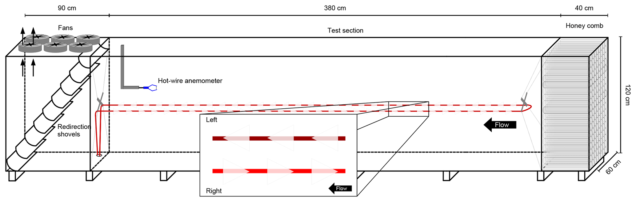
Figure 1Schematic of the low-speed wind tunnel used to test the microstructure approach to detecting wind direction. The subset highlights the cone orientation relative to the mean flow of the tunnel. The FOC with left-pointing cones is cooler than the FOC with the right-pointing cones.

Download

To observe wind direction, we propose a similar approach combining the active heating with microstructures printed directly on the fiber-optic cable (FOC). The underlying assumption is that applying asymmetric microstructures with opposite orientations to paired, actively heated cables induces directional differences in the turbulent flow around the microstructures and thus in the convective heat loss from the FOC to the air. This difference in convective heat loss results in a temperature difference between the two cables that can be sensed by FODS (see Fig. 1).

The convective heat loss from a surface with roughness elements can be written as (Owen and Thomson, 1962)

where ρ is the density of air, c_p is the specific heat of dry air, T_a is the temperature of the air, T_s is the temperature of the fiber, α is an empirical constant related to the roughness of the surface, and Pr is the Prandtl number. m and n are empirical constants. Re_* is the roughness Reynolds length defined as

where u* is the friction velocity, h is the “sand-equivalent height” of the roughness elements or the thickness of the surface layer (Owen and Thomson, 1962), and ν is the kinematic viscosity. Combining Eqs. (1) and (2) yields

Cones pointing into the flow should have a lower equivalent roughness height than cones pointing with the flow as a result of changing from a streamlined shape into a bluff shape. Consequently, actively heated cables with microstructures of opposite orientations should have different cooling convective heat fluxes and resulting temperatures.

The difference in the convective heat flux along each cable is manifested as a temperature difference between the cables from which we define the wind direction signal:

Cables with microstructures pointing into the flow (Fig. 1) should have a smaller (cooling) convective heat flux and higher temperature (T_right) compared to cables with microstructures pointing with the flow, which should have a larger convective heat flux and resulting lower temperature (T_left). In the displayed case (Fig. 1) ΔT>0 would indicate a wind direction from the right, while ΔT<0 indicates a wind direction from the left.

To derive a functional form for ΔT as a function of wind speed, we substitute T_right and T_left into Eq. (1) and subtract the two quantities.

Solving the equation uniquely for T_left−T_right requires knowledge of the form of the friction terms, α_left and α_right. Without an exact expression for these terms Eq. (5) reduces to

Equation (6) suggests that ΔT is nonlinearly related to wind speed, U, since u_* and U are linearly related quantities (Stull, 1988). Equation (6) also implies that U and ΔT have a power law relationship with a negative exponent, as m should be less than 0.5. While expressions for the friction terms are unknown, some sort of nonlinear, decreasing relationship between ΔT and U is anticipated. Accordingly, we also test an exponential decay model as a competing representation of the nonlinear relationship.

2.2 Instruments and wind tunnel

The microstructure approach to distributed observations of wind direction was tested in a controlled wind tunnel environment. The wind tunnel was designed to provide small turbulence intensity for low velocity flows. The suck-through wind tunnel test section was 3.0 m long, 0.6 m wide, and 1.2 m tall. At the entrance of the wind tunnel the flow was straightened and external turbulence was combed out using a honeycomb section made from 0.20 m long pipes with a 0.05 m radius. The flow was allowed to settle over 0.6 m before entering the test section. The tunnel was lined with 0.03 m thick insulating polyurethane boards to eliminate spatial differences in surface temperature and thus provided a coherent radiative environment within the tunnel, which minimizes differences in the longwave radiative transfer that arises from even subtle differences in surface temperature and emissivity. Deviations of longwave radiation parallel to the cable can cause artifacts in the DTS.

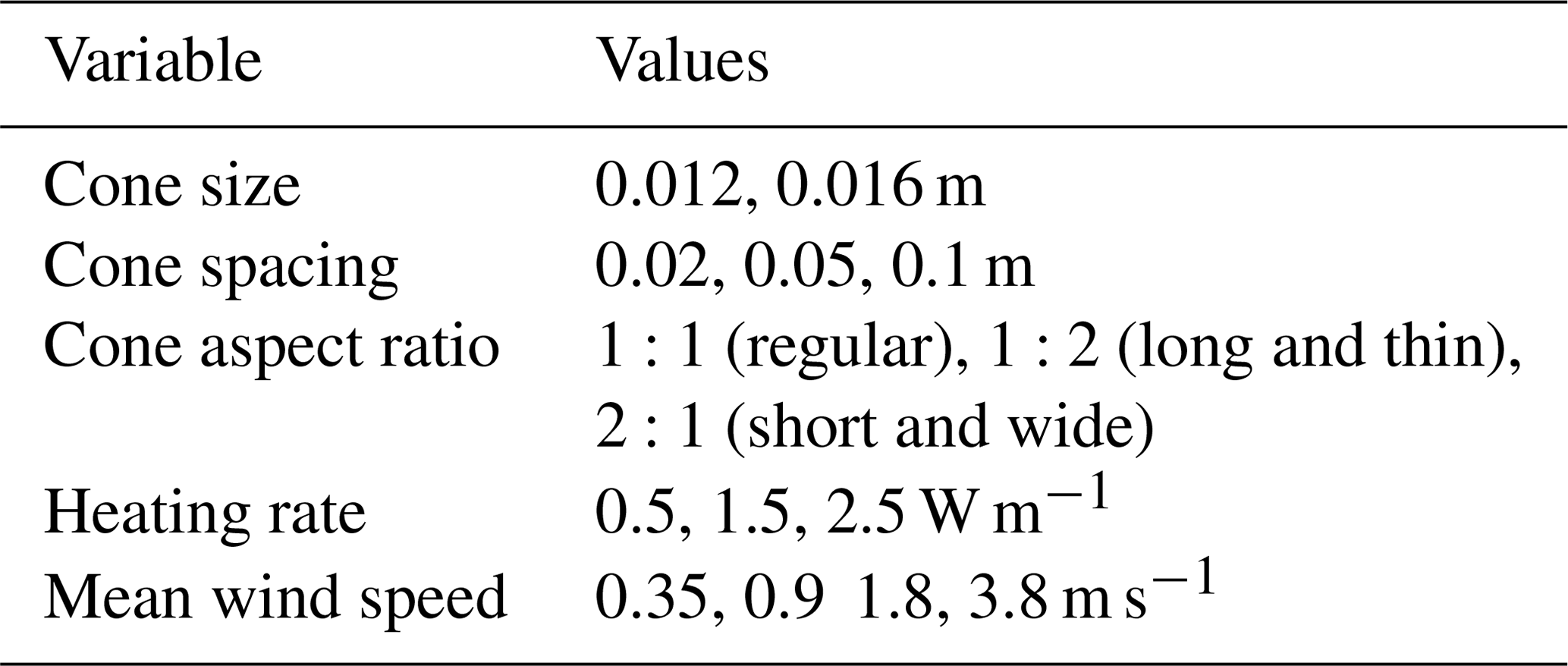
A sonic anemometer (Model CSAT3, Campbell Scientific Inc., Logan, UT, USA) was used to pre-characterize the flow by moving the instrument throughout the tunnel both in transects along the tunnel and in selected planes orthogonal to the along-tunnel dimension. The tunnel was controlled to yield consistent wind speeds for each test with along-flow velocities as given in Table 1. Each parameter was tested with 10 min of observations using a flow that did not vary in time. The center of the wind tunnel was free from the influence of a shallow wall boundary layer. At the back of the tunnel there was some enhancement of turbulent mixing due to deflection towards the fans, which was excluded from further analysis. Horizontal turbulent intensity, the ratio of the standard deviation of the horizontal wind components to the mean velocity, varied between 0.005 and 0.01 for the lowest to highest wind tunnel velocities. The friction velocity along the central axis of the wind tunnel ranged from 0.0025 m s⁻¹ for the lowest wind speeds to 0.02 m s⁻¹ for the highest wind speeds. The turbulence within the tunnel was substantially lower compared to atmospheric flows (e.g., Friedrich et al., 2012) and may impact direct transfer of wind tunnel results to field conditions.

Table 1Tested parameters values.

Download Print Version | Download XLSX

The time-averaged wind speed during the 10 min tests with the FOC was monitored using a one-dimensional hot-wire anemometer (Model, TA300, Trotec, Heinsberg, Germany) with a precision of ±0.2 m s⁻¹. To provide an independent measurement of the fiber temperatures, a high-resolution thermal infrared camera was used to record its brightness temperature (Model PI640, Optris, Berlin, Germany). The camera observes the wavelengths of 7.5 to 13 µm with a pixel resolution of 640×480 and an accuracy of ±2 ^∘C. The camera was placed on the floor of the wind tunnel looking up at the FOCs such that the pixel resolution was 0.00025 m. Pictures of the fiber and microstructure brightness temperatures were acquired at 1 Hz and averaged over 10 s. In order to avoid angular effects of the emitted thermal radiation, the cones and fiber were coated with infrared paint (Washable thermographic paint for special applications, LabIR, Pilsen, Czech Republic) that has a known emissivity of 0.94 to 0.97 for viewing angles 60 to 5^∘, respectively.

2.3 Fiber-optic array

One continuous FOC was deployed in the test section, parallel to the flow within the wind tunnel (Fig. 1). The cable was mounted within the tunnel using square aluminum crosses with a width of 7.5 cm and was gently looped around the back of the crosses to avoid sharp bends which cause a signal loss (Selker et al., 2006). The FOC had a 0.82 mm stainless steel sheath with a 0.15 mm PVC coating, yielding a total outer diameter of 1.12 mm and the actual fiber-optic cable was loosely buffered and gel-filled (Model C-Tube, Brugg, Brugg, Switzerland). The cable was heated electrically by applying a current to the high-resistance (2.3 Ω m⁻¹) stainless steel sheath. Microstructures were mounted in opposing directions on the looped cable (zoomed in region Fig. 1).

Fiber temperature was observed using a high-resolution DTS instrument (Model 5 km Ultima, Silixa, London, UK). This DTS device is capable of fine-scale distributed temperature observations with a sampling resolution of 0.127 m with a temporal resolution of ≈1 s. The implications of instrument noise on the wind direction approach is discussed in Sect. 3.3.

The intensity of the back-scattered light was converted to a temperature using calibrated parameters that vary with instrument temperature and fiber properties. We explicitly calculate these parameters through a matrix inversion of the back-scatter equation using three reference sections with a single-ended approach (Hausner et al., 2011). This calibration technique eliminates effects from differential attenuation and instrument properties that can vary with time.

The reference sections are composed of warm and cold calibration baths. The cables were deployed in the calibration baths both prior to entering the wind tunnel and after the fiber exits the tunnel, yielding two temperatures at four locations along the fiber. Three of these calibration sections were used to solve for the calibrated parameters with the fourth withheld for characterizing the instrument uncertainty. Each reference bath was well-mixed using aquarium pumps to avoid stratification. The fiber was loosely coiled within the baths such that they did not contact the bath walls. Two class-A PT100s, with an accuracy of 0.15 ^∘C, were deployed in each calibration bath. After calibration, the DTS had a root mean square error of 0.61 ^∘C (n=4 300 000) when evaluated against the temperature of the reference bath, in line with the published accuracy from the manufacturer. We used this error as an estimate of the instrument uncertainty (Sect. 3.3).

2.4 Numerical simulations

Computational fluid dynamics (CFD) simulations were completed to inform the initial design decisions of the microstructures and to verify the observed heat transfer mechanism (Sect. 3.4). We used the OpenFOAM computational fluid dynamics software (https://www.openfoam.com, last access: 30 March 2020) with the simpleFoam solver and the standard k–ϵ turbulence model for doing a 3-D simulation of the flow along a fiber with microstructures. The simulations were done using a long enough piece of fiber such that the flow could adjust to the microstructures. We tested the heating rate, microstructure size, aspect ratio, and spacing each at a variety of wind speeds. The initial CFD simulations allowed the targeting of a specific range of variables. This CFD approach does not simulate heat transfer, so effects like buoyancy are neglected, which is a reasonable assumption for such small temperature perturbations (Zeitoun et al., 2011).

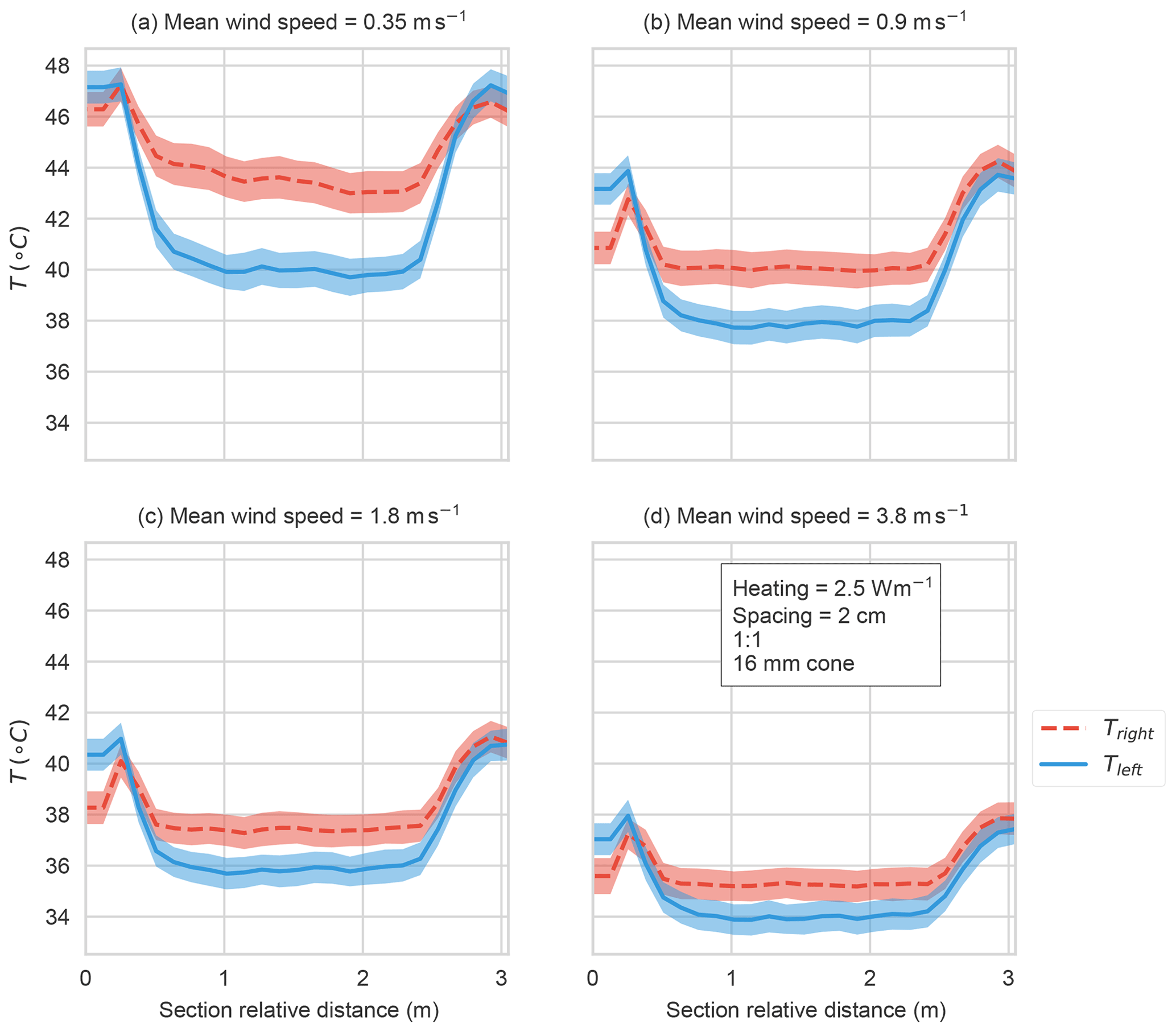
Figure 2Time-averaged temperature (10 min) along the test section in the wind tunnel for a horizontal wind speed of (a) 0.35, (b) 0.9, (c) 1.8, and (d) 3.8 m s⁻¹ for the parameters listed. The standard deviation of temperature in time for each point along the FOC is shown in the filled colors. The cones are only present between 0.75 m and 2.25 of the tunnel section. The mean wind direction is in the positive x direction.

Download

3.1 Temperature differences

The results confirmed our initial assumption of directionally sensitive heat loss, and thus cable temperatures, from the cones pointing in different directions (see Fig. 2 for an example for a single test of cone spacing, size, aspect ratio, and heating rate as a function of wind speed). The largest temperature difference between cables coincides with the location of the microstructures (between 0.75 and 2.25 m). At the beginning (x=0 m) and end (x=3 m) of the test section, the cable temperature exhibits artifacts caused by the support crosses that are used to mount the fiber in the tunnel. The microstructure fibers exhibit a uniform temperature within the test section except at the lowest wind speed, in which a decrease in temperature is observed with length along the tunnel, perhaps as a result of unorganized turbulence within the tunnel at these low wind speeds. The heated fibers cool as the wind speed is increased, as expected.

At all wind speeds in the region with cones, the fiber with cones pointing left (Fig. 1) has a lower temperature than the fiber with cones pointing right. ΔT is the largest at the lowest wind speeds and becomes small enough at the highest wind speed that the fiber temperatures overlap (shaded regions in Fig. 2d). The effect of the uncertainty in the ΔT signal is discussed further in Sect. 3.3. The reduction in the ΔT signal with higher wind speeds may be caused by the enhanced roughness from both microstructure orientations being unable to increase the sensible heat flux beyond some maximum value.

When determining the temperature difference, we examine the test section in which the cone signal is not affected by edge effects (0.75 to 2.25 m along the tunnel). The temperature signal for both fibers is linearly interpolated to a common x coordinate along the tunnel.

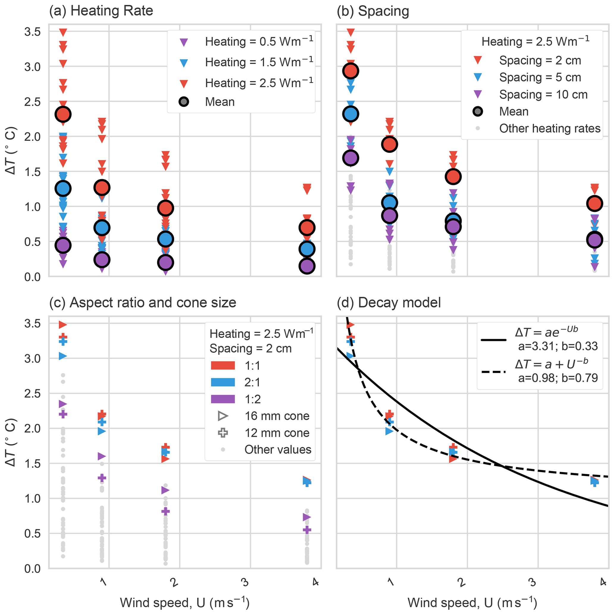
Figure 3The ΔT for all combinations of cones and heating rates (see Table 1). The data are stratified using the variable with the largest impact, i.e., temperature difference between coned cable sections pointing in different directions. (a) All temperature differences as a function of wind speed classified by heating rate. (b) The highest heating rate is selected (red points in a) and data are classified according to the spacing between cones. Data with lower heating rates are shown in grey. (c) The 2 cm spacing and highest heating rates (red points in a and b) are selected and then classified according to the cone aspect ratio. The 12 mm cones are marked with pluses, and the 16 mm cones are marked with right-pointing triangles. All other heating rates and cone spacings are shown in grey. (d) The best performing parameters are fit with an exponential and power law model (see Sect. 2.1 for details).

Download

3.2 Optimizing the microstructure configuration

The temperature signal is defined as the mean difference, in both time and space, according to Eq. (4). A positive ΔT is expected, as the fiber with left-pointing cones should be warmer than the fiber with the right-pointing cones. The tested parameters were stratified from the most influential (Fig. 3a) to least influential (Fig. 3c) factors. A hyperbolic and an exponential model were fit to the set of best performing parameters (Fig. 3d).

The most influential parameter was the cable heating rate. A heating rate between 1.5 and 2.5 W m⁻¹ yields the largest ΔT with a mean difference of approximately equal to 1.0 K at the lowest wind speed and 0.3 K at the highest wind speed (Fig. 3a). Certain combinations of microstructure properties with higher heating rates have a smaller ΔT than different combinations of microstructure properties with a lower heating rate. However, a larger heating rate leads to a larger ΔT for a fixed combination of cone size, spacing, and aspect ratio.

The cone spacing was the second most influential factor, largely due to the smallest cone spacing of 0.02 m (Fig. 3b). The mean ΔT values for the 0.05 and 0.1 m spacing were indistinguishable at higher wind speeds, while the 0.02 m spacing resulted in the highest ΔT. The other parameter values tested, such as cone aspect ratio and size, had a limited effect (Fig. 3c). The exception was the aspect ratio, width : height, of 1:2, which led to the smallest ΔT as the other two aspect ratios converged to the same ΔT for higher wind speeds. At lower wind speeds, the effect of cone size and aspect had an inconsistent effect. For instance, the 0.016 m cones had the largest temperature difference for the 1:1 cones and the smallest difference for the 2:1 cones. This ordering reversed itself at higher wind speeds (Fig. 3c). However, these differences were well within the observational uncertainty for the DTS device and should not be interpreted. From this we conclude that any combination of the 0.012 and 0.016 m cone sizes and the 1:1 and 2:1 aspect ratios was appropriate for developing the distributed wind direction observation system.

We further evaluated whether ΔT is well-described by a power law or exponential decay relationship with wind speed. The power law function outperformed the exponential decay as it has smaller residuals and a lower uncertainty in the fit parameters. Additionally, it was able to describe all sets of tested parameters as a function of wind speed, albeit with different parameter values, while the exponential fit cannot (not shown). The results here suggest that the basic relationship shown in Eq. (6) is applicable. It should be noted that both functions have problematic limiting behavior as the wind speed approaches zero. Further work will be necessary to identify a minimum wind speed threshold at which ΔT becomes significantly nonzero.

3.3 Certainty in estimating the wind direction signal

The wind direction signal, ΔT is subject to a non-negligible uncertainty from the DTS device. The uncertainty for ΔT is formulated as

where δ_T is the uncertainty in the ΔT signal and σ_DTS is the mean standard error derived from the DTS reference thermometers immersed in the calibration baths of uniform temperature. For the DTS device used in this study, the mean standard error is 0.61 ^∘C (Sect. 2.3) yielding an uncertainty δ_T=0.81 ^∘C. From this it follows that any ΔT≤δ_T cannot be distinguished from noise.

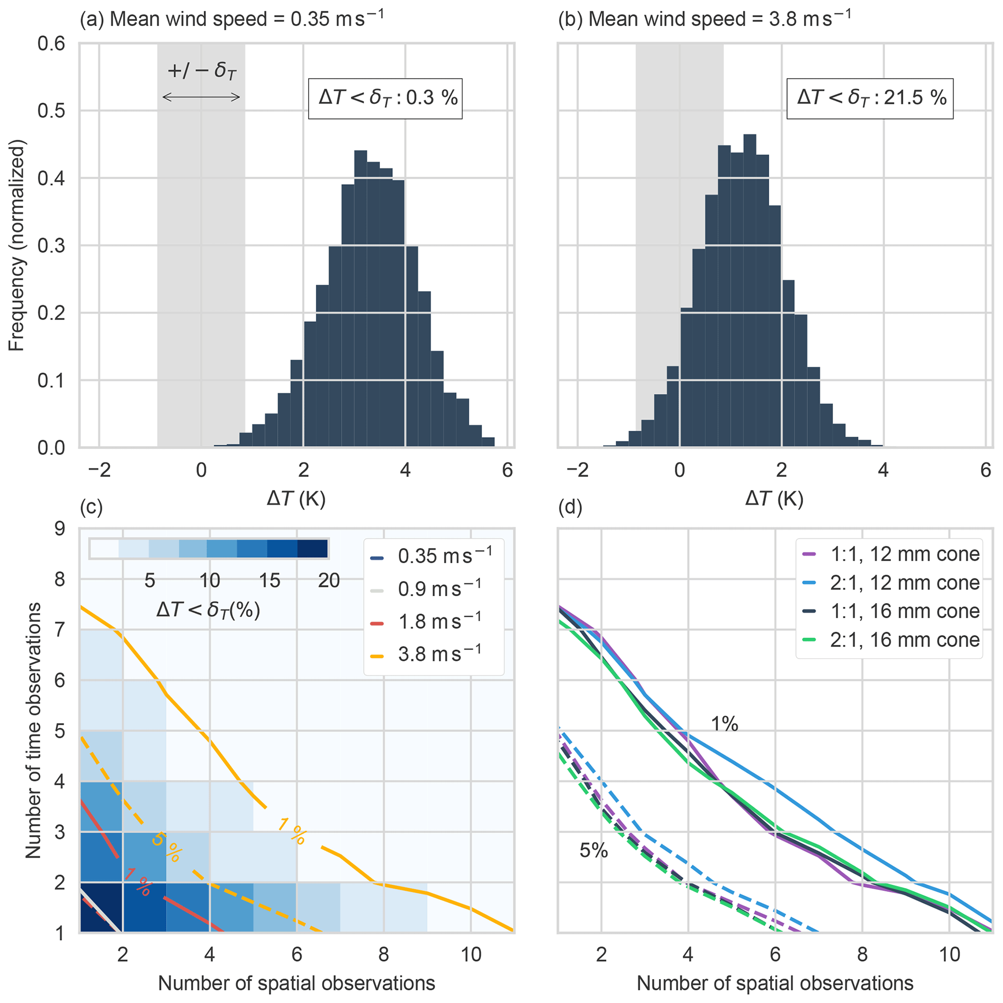
Figure 4The distribution of temperature differences between cables with opposing cone orientations for the 16 mm, 1:1 cones with 2 cm spacing and a heating rate of 2.5 W m⁻¹ for (a) a wind speed of 0.35 m s⁻¹ and (b) a wind speed of 3.8 m s⁻¹. The grey region indicates the uncertainty, δ_T. The percentage of observations with ΔT<δ_T is indicated. (c) A 2-D histogram of the percentage of ΔT<δ_T as a function of averaging interval in time and space for the highest wind speed (same data as in b). The contours for the 1 % and 5 % thresholds are indicated for each wind speed. Note that the 0.35 m s⁻¹ wind speed is always below the 1 % threshold. (d) The 1 % and 5 % contours for the acceptable cone aspect ratios and sizes at the highest wind speed.

Download

The distribution of ΔT in both time and space (n=20 700) for a given experiment was normally distributed around the mean difference (Fig. 4a, b). The strength of the wind direction signal was inversely related to wind speed (Fig. 2) and as a consequence the fraction of ΔT≤δ increased with the wind speed. At the highest wind speed tested, some ΔT values even changed sign, which would result in an incorrect wind direction estimation (Fig. 4b).

One strategy for improving the accuracy of the wind direction signal is to average the temperature signal from both cables in time and space prior to computing ΔT. A running average of temperature was calculated using a variable number of time (1 s) and/or space (0.127 m) observations (Fig. 4c, d). Averaging the temperature signals over longer temporal and spatial intervals than the native resolution of the DTS device reduced the fraction of ΔT signal below the instrument accuracy and hence increased the fraction of observations suitable for wind direction determination (Fig. 4c). For a given set of microstructure parameters, all wind speeds benefit from averaging the FODS signals. The exception is the lowest wind speed of 0.35 m s⁻¹, which effectively always yielded a ΔT larger than δ_T (Fig. 4c). In this case, the averaging reduces the temporal resolution of the wind detection calculations. All acceptable cone size and aspect ratios found in Sect. 3.2 had similar responses to averaging the FODS signal except the 0.012 m cones with a 2:1 aspect ratio yielded slightly greater uncertainty than other combinations (Fig. 4d).

Any averaging reduces the resolution of the method. Fewer time intervals are necessary for improving the certainty in the ΔT signal compared to spatial averages for all wind speeds (Fig. 4c). However, an interpretation solely based upon number of averaging intervals may be misleading as the wind direction method is aimed at observing atmospheric turbulence, especially for the weak-wind boundary layer featuring short-lived and small-scale motions. Instead, we seek to find spatial and temporal averages that facilitate the observation of mean direction for a typical eddy length scale during those conditions. Taylor's hypothesis (Taylor, 1938) is commonly employed for estimating the eddy scale that can be resolved with a particular instrument resolution. With Taylor's hypothesis timescales can be converted into spatial scales by assuming a relationship between temporal and spatial gradients through

where U is the mean wind speed, ℓ is the spatial scale of a turbulent eddy, and τ is the timescale. At a wind speed of 4 m s⁻¹, a 4 s average results in observing eddies of length scale of ≈16 m. This eddy length scale is larger than those commonly found in the weak-wind boundary layer, whereas a spatial average with n=10 observations equates to an observation every 1.27 m. Using the DTS temporal resolution, for the same 4 m s⁻¹ wind speed, an eddy of length scale ≈4 m can be observed. For this reason, improving the certainty in ΔT at higher wind speeds through spatial averaging is recommended.

Figure 5The brightness temperature of the fiber-optic cables with (a) left- and (b) right-pointing cones for the 12 mm, 1:1 cones with 2 cm spacing and a heating rate of 2.5 W m⁻¹ for a wind speed of 0.9 m s⁻¹. (c) The average of the three warmest pixels in each horizontal row is provided to better demonstrate the spatial pattern of temperatures along the fiber. The grey shading is to visually line up the cones in (a)–(c). (d, e) Turbulence kinetic energy (TKE) computed from the CFD simulations for the same experiment as in (a) and (b) with (f) the difference in TKE between the two orientations. The difference in TKE was not physically meaningful in the region with a cone in either (d) or (e) and is excluded in (f). The subset arrows indicate the direction of the mean flow.

Download

3.4 Explaining the physical mechanism for directional heat loss

To provide an independent verification of the FODS signals and investigate the mechanism behind the observational principle, a thermal infrared camera was employed to observe the fiber and cone brightness temperatures (Fig. 5a–c). The use of a paint with a relatively constant emissivity with viewing angle allows a comparison of brightness temperature between different parts of the microstructure fiber-optic cable setup. The brightness temperature revealed the fine spatial structure of temperatures across the microstructure-cable, from which we inferred differences in the convective heat loss. The brightness temperatures for both the left- and right-pointing cones were cropped from the larger image (Fig. 5a, b) using a threshold value. The differences in temperature between the left- and right-pointing fibers were driven by differences in temperature in two locations. The base of the cones was the coolest part of the cable–cone system with the base of the left-pointing cones being ≈2 ^∘C cooler than the base of the right-pointing cones (Fig. 5c). The cable immediately behind the right-pointing cones, in the lee of the flow, was the warmest point along the fiber and was warmer than the equivalent segment on the left-pointing cones by >2.5 ^∘C. This difference in temperature decreased with length along the cable towards the next pair of cones.

The brightness temperatures suggested that two factors explain the directional sensitivity of the heat loss to the microstructures. First, the low temperatures on the base of the left-pointing cones imply an enhancement of turbulent exchange at the base of the cone relative to the right-pointing cones. Secondly, the high fiber temperatures behind the right-pointing cones imply that the right-pointing cones are sheltering the cable in their lee, reducing the cooling by limiting the convective heat flux. The sheltering effect may partially explain why our findings for the cone spacings of 0.05 and 0.1 m were indistinguishable (Fig. 3b), as the sheltering occurs over a distance of approximately 0.01–0.02 m. As the spacing increases past the range in which the sheltering occurs, the fibers with right- and left-pointing cones converge to the same temperature (not shown).

The two turbulence features suggested in the brightness temperatures are further demonstrated using CFD simulations for the same fiber setup shown in Fig. 5a and b. The simulated turbulence kinetic energy (TKE) is used as a proxy for the convective heat exchange. TKE is defined as

where u, v, and w are the three orthogonal wind velocity components and the ^′ denotes the temporal perturbation from Reynold's averaging. The differences in TKE corresponded to the features found in the brightness temperature. The left-pointing cones substantially enhanced the turbulent exchange at the base of the cones compared to the right-pointing cones (Fig. 5f). Additionally, the right cones strongly reduced TKE in the lee of the cones (Fig. 5f). Both effects caused the left-pointing cones to be subject to enhanced convective heat exchange relative to the right-pointing cones. The right-pointing cones did provide a small enhancement of turbulent exchange further along the fiber, past the region in the lee of the cone (blue colors in Fig. 5f). This enhanced turbulent exchange was also apparent as the brightness temperature of the right-pointing cones decreased from the base of one cone to the tip of the next one (Fig. 5c). However, this small increase in turbulent exchange was not large enough to overcome the reduction in turbulent exchange directly in the lee of the cones. Both the CFD modeling approach and the independent experimental brightness temperatures confirmed that the wind direction signal from the oriented microstructures results from differences in the convective heat exchange generated by the microstructures.

3.5 Remaining questions and future work

This study only demonstrated the ability to observe wind direction within one dimension. Convolving the FODS wind direction observations along orthogonal directions into a fully three-dimensional wind field is a substantial challenge and beyond the scope of this proof-of-concept study. The angle of attack of the mean wind direction along the fiber will influence of the wind direction signal, similar to issues with observing wind speed with FODS (Sayde et al., 2015; Pfister et al., 2019; Ramshorst et al., 2019). Exploring the effect of wind attack angle was not possible given the size and aspect ratio of the wind tunnel used in this study. The ability to detect mean wind direction is useful, but developing a flow sensor for studies of atmospheric turbulence also requires the ability to detect rapidly changing wind vectors. The cone/cable system has some thermal inertia that creates a lag in reaching an equilibrium ΔT. This study only highlights the ability to measure time- and space-averaged flow, which may not be sufficient to resolve the energy-containing eddies for weak-wind boundary layers. Additional work is necessary for determining the time response of the wind direction signal. Finally, the flow explored in this proof-of-concept study has a lower turbulence intensity than atmospheric flows. Deployments in real atmospheric flows may require a larger heating rate or further averaging in order to observe a meaningful ΔT. These considerations need to guide future work to enable true three-dimensional observations of wind speed and direction. The method for detecting wind direction depends on the temperature difference between two cables that are identical besides the cone orientation. A number of factors, for instance cable type, size, and the number of optical cores, may cause this temperature difference to vary. Understanding these factors will be critical to developing a robust, empirical relationship between the directionally sensitive temperature signals and wind direction.