2.1 CFD study

CFD simulations were used to develop a quantitative understanding of fluid flow around the vehicle and to evaluate flow under a wider range of conditions than is feasible in a field study. These data were used to investigate how the shape of the vehicle impacted measurement accuracy when the vehicle was travelling in the upwind and crosswind directions. We defined measurement bias as the difference between the inlet velocity and the velocity magnitude at the anemometer location. We created two sets of simulations in ANSYS Fluent, the first of which was designed to evaluate the flow field under varying vehicle speed and the second to explore the flow field under varying wind yaw angles.

Figure 1Truck model geometry replicating a 2016 Toyota Tacoma field vehicle.

Download

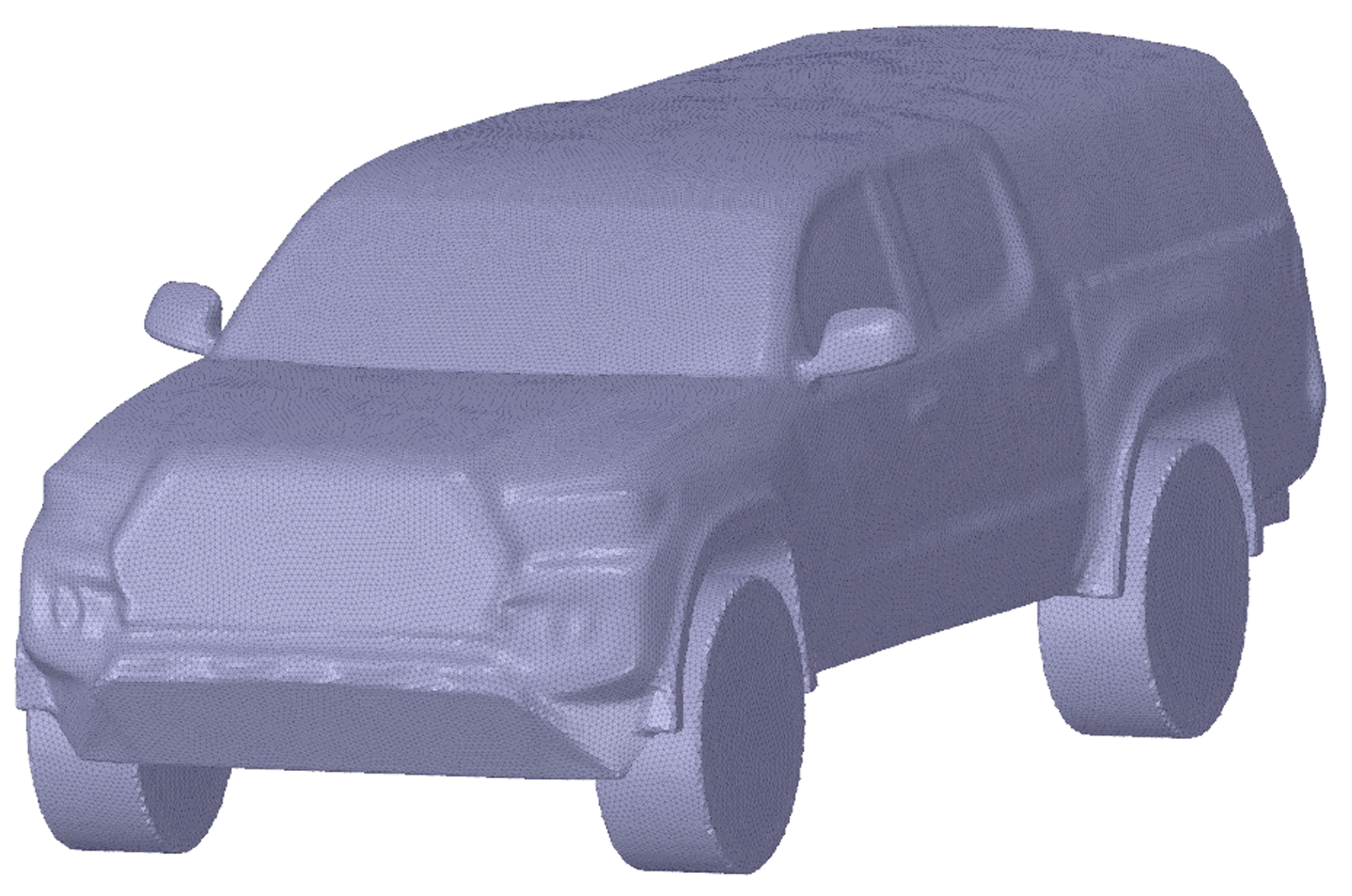
The vehicle geometry was that of a 2016 Toyota Tacoma model equipped with a bed cap cover, similar to that used in Atherton et al. (2017), and modified to have a smooth underbody with simplified tires. The vehicle model (Fig. 1) was enclosed in a virtual wind tunnel extending 25.4 m above, ahead, behind, left, and right of the truck model. The computational domain of the wind tunnel was 56.2 m in length, 53.0 m in width, and 28.2 m in height, with just under 84 000 m³ of air volume. The wind tunnel was designed to have a large width so that the vehicle speed and yaw angle could be evaluated in a consistent manner across simulations. A fine-resolution tetrahedron assembly mesh was generated in the ANSYS workbench package with 4.6 million cells, ranging from a fine scale adjacent to the surface of the truck to coarse farther away. The computational wind tunnel was defined to have a velocity-based inlet (1 % turbulence intensity) and a pressure-based outlet. We modelled the road and truck surfaces as stationary walls with no slip condition, as well as the top and sides of the tunnel with symmetry boundary conditions.

A drag coefficient comparison with the manufacturer's specification was used to compare the performance of three turbulence models. We calculated the drag coefficient of the truck model using a realizable two-equation k-ε model with non-equilibrium wall functions, a two-equation k-ω shear stress transport (SST) model, and a four-equation transition SST model. All turbulence models are built into the ANSYS software and based on the steady-state formulation, Reynolds-averaged Navier–Stokes (RANS) equations. In simulations comparing the turbulence models, the drag coefficient was calculated using an inlet velocity of 22.2 m s⁻¹ (80 km h⁻¹) and the vehicle's projected frontal area of 2.819 m². The drag coefficient was determined when the change in C_D was less than 0.001. The ΔC_D column was determined by comparing the calculated drag with the 2016 4×4 double-cab Toyota Tacoma specification value for C_D of 0.386 (Toyota USA, 2016). The results of the C_D comparison are displayed in Table 1. All turbulence models produced drag coefficients greater than the manufacturer's reported value. The addition of the cap on the truck model may have increased the frontal area, resulting in this slightly larger drag coefficient. The k-ε model provided a C_D value within 6 % of Toyota's specification value and was chosen as the most suitable model for our computational mesh.

Previous studies (Holloway et al., 2009; Roy and Srinivasan, 2000; Yang and Khalighi, 2005) have used k-ε models for the purpose of external vehicle aerodynamics. The k-ε models use two additional equations to solve the RANS equations, one for turbulent kinetic energy (k) and one for the turbulent kinetic energy dissipation rate (ε) (Roy and Srinivasan, 2000). The realizable k-ε model with non-equilibrium wall functions was advantageous for this study. Non-equilibrium wall functions are sensitized to adverse pressure gradients and predict flow behaviour in turbulent boundary layers better than the traditional k-ε model, which is limited in cases of larger adverse pressure gradients (Parab et al., 2014). The k-ε model has been previously used to study external vehicle aerodynamics. Holloway et al. (2009) compared a steady k-ε model with two transient turbulence models, concluding that all of the models capture the general trends in the flow field aft of the cab of a pickup truck. In a study comparing CFD and experimental data, similar flow structures were observed from a steady k-ε CFD model and time-averaged wind tunnel test experiments when comparing velocity planes parallel to the ground (Yang and Khalighi, 2005). The pickup truck models in both these studies had an open bed. In our study, the model we were exploring has a cap on the bed. The flow field around a pickup truck is more complex than the flow around an SUV or sedan because of wake interactions (Yang and Khalighi, 2005). The cap on the truck bed eliminates the pressure drop that occurs on pickup trucks when the air flows over the cabin and into the bed. Our motivation for placing an anemometer atop a pickup is to assist vehicle-based gas monitoring systems (Atherton et al., 2017; Baillie et al., 2019; O'Connell et al., 2019) measuring gas emissions to achieve practical placement and further calibration practices. In these studies, the anemometer was mounted above a truck cap. Because of the differing vehicle shape from an open bed pickup truck, k-ε performance in the drag comparison, and performance in other studies, we have selected the k-ε turbulence model as appropriate for our analysis in the velocity field above a capped pickup truck.

Table 1Drag comparison of three turbulence models with an inlet velocity of 22.2 m s⁻¹. The drag coefficient (C_D) for each turbulence model is reported with the number of iterations required to achieve a solution and the percent difference (ΔC_D) from the manufacturer's reported value (C_D) of the vehicle model.

Download Print Version | Download XLSX

In the first set of simulations, the above model was used to investigate the flow over the vehicle at speeds ranging from 40 to 100 km h⁻¹ in 5 km h⁻¹ increments. All simulations were performed in ANSYS Fluent 17.2 and were run in parallel using 32 cores dispersed over two nodes using 2.2 GHz Opteron or Intel Xeon 2.7 GHz clusters made available by Compute Canada.

In the second set of simulations, eight additional computational domains were created to explore the effects of wind yaw angle, each representing a different wind yaw angle for the truck. In each case, the truck's longitudinal axis was rotated so that the inlet was perpendicular to the yaw angle direction of flow. The computational domain was to made to extend the same 25.4 m in each direction as the original tunnel. The truck was rotated counterclockwise in 5^∘ increments to provide models between 5 and 40^∘ inclusive. The symmetry plane of the truck was used to simulate the corresponding yaw angles of 320 to 355^∘ inclusive. We assumed that the wind atop the truck on the passenger side at 5^∘ will represent the same wind that the driver side of the truck experiences if the truck was rotated 355^∘. We used the additional computational domains to test all combinations of yaw under inlet speeds ranging from 40 to 100 km h⁻¹ in 5 km h⁻¹ increments.

2.2 Field measurements

The field experiments were designed to validate the CFD results, using stationary anemometer measurements as a control comparison for truck-based anemometer measurements. For comparison with CFD, it was necessary to obtain truck-based wind measurements from a range of yaw angles. Field tests were carried out using a 3.2 km by 3.2 km driving route, with a stationary anemometer positioned near each corner in order to compare truck-based anemometer measurements under headwind, tailwind, and side wind conditions with those acquired by the stationary anemometers. The stationary anemometers were placed on the corners to provide opportunity for comparison with both legs of the straightaway. This ensured that we would have data for comparison with each leg should an anemometer malfunction. The square route also provided vehicle-based measurements for tailwind conditions, where stationary anemometers recorded wind direction opposing the vehicle path. The terrain was flat, treeless, and nearly devoid of infrastructure, and we experienced minimal traffic.

In summer 2017, we drove the route at speeds of 40, 50, 60, 70, and 80 km h⁻¹. Our hardware consisted of an RM Young 86004 ultrasonic anemometer mounted on a 1.2 m tall mast above the cap of a 2016 Toyota Tacoma, with a total height of 3 m above the surface. The anemometer was positioned 0.5 m from the longitudinal axis of the truck on the driver's side and 0.3 m behind the start of the truck's cap, in the location of the roof racks. A Campbell Scientific CR1000x data logger recorded time, wind speed, wind direction, and instantaneous geolocation from a Garmin GPS 18X, at 1 Hz. Four stationary tripod-mounted Decagon Device DS-2 sonic anemometers measured wind speed and wind direction at a height of 3 m above the ground. The tripods were located approximately 300 m clockwise from each corner to allow for the truck to be travelling at a constant speed when passing the stationary instrument. Measurements of time, wind speed, maximum gust, and direction were recorded with a Decagon Device Em50 data logger in 1 min intervals at the same time we were driving the route. The Decagon anemometer model was selected based on cost effectiveness, and the RM Young model was selected for its ability to measure high wind speeds, which are necessary for the mobile wind measurements. A schematic describing the field experiment is displayed in Fig. 2. The calculated vehicle bearing measurements showed that the roads used in the square route were within 2^∘ of the north, south, east, and west directions.

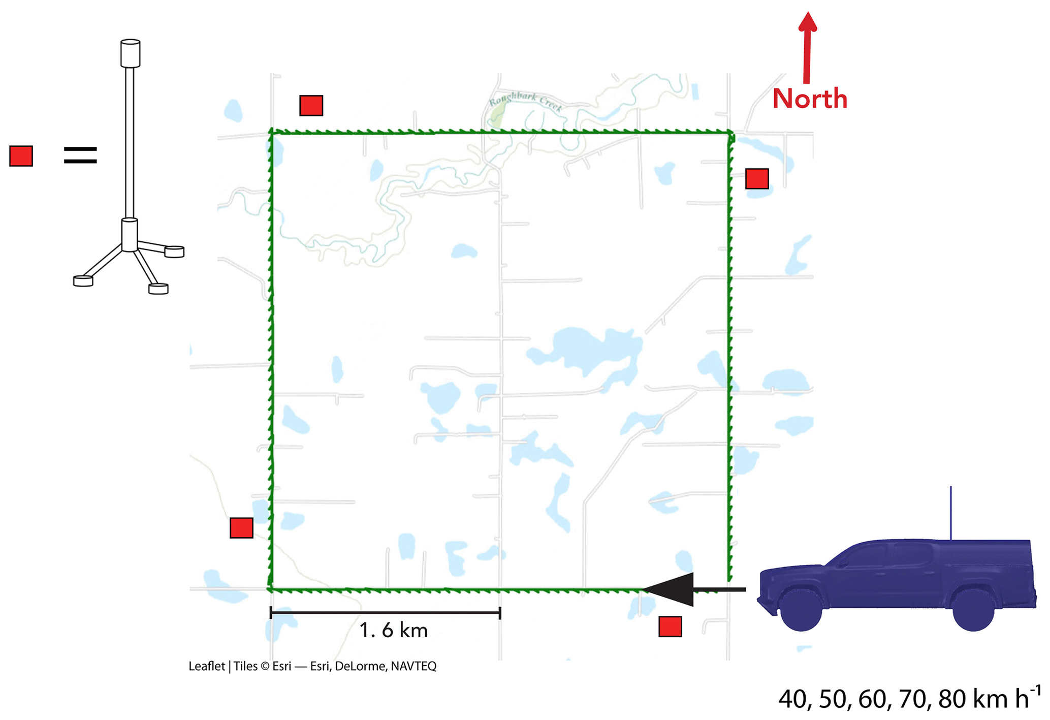
Figure 2Field schematic displaying the location of stationary anemometers, the site and the vehicle path. The vehicle path was driven clockwise and repeated at speeds of 40, 50, 60, 70, and 80 km h⁻¹. Map data: ©Esri – Esri, DeLorme, NAVTEQ.

To explore the effects of the anemometer height above the truck, we repeated tests with the addition of a secondary anemometer at a lower position of 0.3 m above the truck (2.1 m above the ground) and 0.4 m from the longitudinal axis of the truck on the driver's side.

The vehicle speed and bearing measurements were computed from recorded 1 Hz geolocation measurements. The field measurements that corresponded to geolocation measurements calculating vehicle speeds that deviated more than 2.5 km h⁻¹ from the implemented cruise control speed or 5^∘ from the designated vehicle course were removed. The vehicle anemometer measurements from each field test were corrected to remove the vector of the vehicle's motion. To correctly compute true winds, vehicle-based wind must be corrected for the vehicle's motion over the fixed earth. The vehicle vector has a direction equivalent to the vehicle's course over the ground and a magnitude equivalent to the vehicle's speed over the ground (Smith et al., 1999). The 1 Hz wind direction and wind speed measurements from the truck anemometer were each used to create the real and imaginary components for the wind vector, with the coordinate system aligned so that the front of the truck was 0^∘. The wind vector was translated to match the truck's coordinate system, with north as 0^∘. We calculated the vehicle's course over the ground using the 1 Hz GPS coordinates to obtain a vector of equal magnitude and opposite direction to the frontal wind induced by the vehicle's motion (F). We compute the meteorological wind vector (W) by subtracting the frontal wind induced by the vehicle's motion (F) from the raw anemometer-measured wind vector (A). The calculation is presented in Eq. (1). The computation comes from the method calculating the meteorological true wind from a moving vessel presented by Smith et al. (1999).

3.1 CFD results

The CFD simulations provided a quantitative description of the airflow surrounding the vehicle. Velocity fields were the interest of this study, and we observed that wind yaw angle has a more pronounced effect on the wind speed bias than the vehicle speed does. This result was expected as vehicles are designed to be aerodynamic in the forward direction of motion.

The first set of simulations was evaluated to explore the effect of vehicle speed on wind measurement bias. In each computational domain, we found that the wind bias scaled with vehicle speed and the amount of bias (slope) differed with the location above the vehicle. Similarly, Houston et al. (2016) found that CFD calculated velocities for sensors positioned atop a van scaled linearly with along-axis speed. Our location of interest for placing anemometers was on the truck's bed cap. Velocity contours were computed for the longitudinal axis of the truck and for the lateral plane on the truck located 30 cm from the end of the cab, which was the location of the roof racks on which the anemometers were mounted in the field test.

Figure 3 displays a velocity contour for the overestimation of the speed along the longitudinal axis of the truck. In this plane, we found that the velocity flowing over the truck was less than the inlet speed at small heights above the truck cabin and cap. In the location of the roof racks, the flow velocity was less than the inlet speed at heights lower than 17 cm above the truck. At 17 cm, the velocity flow transitioned to become larger than the inlet speed. The velocity gradient with respect to height was largest in the region where the flow transitioned to becoming larger than the normalized wind speed, and it decreased with increasing height. The magnitude of flow acceleration was greatest immediately above 17 cm and decreased with increasing height above the truck. This observation is similar to a conclusion by Moat et al. (2005), stating that shipboard anemometers should not be placed close to the line of equality (where measured wind speed equals true wind speed) as large pressure gradients are present in this region. The line of equality would be expected to move vertically to some degree, according to the ground speed and/or wind speed.

The second set of simulations in this study are of particular interest because they evaluate the flow field under crosswind conditions. Many previous CFD and wind tunnel studies (Holloway et al., 2009; Yang and Khalighi, 2005) examine the flow field resulting from inlets which direct the airflow along the longitudinal axis of the vehicle. Aside from Houston et al. (2016), we have not found studies using CFD to conduct crosswind experiments to study the flow field around a vehicle. In performing this analysis, we observed that the change in wind speed magnitude from the inlet increased along with the wind yaw angle between the inlet and the vehicle's longitudinal axis. The flow above the truck displayed a profile where decelerating flow was found below a region of accelerating flow before reaching the undisturbed velocity flow. The maximum magnitude of flow acceleration that occurs above the deceleration region increased with increasing yaw angle. Figure 4 shows the profile of velocity contours in the lateral plane of the truck along the location of the roof racks on the truck when the truck is exposed to frontal, 15^∘ passenger, and 30^∘ passenger wind. When exposed to large yaw angles, the wind bias over the truck at low heights can be 20 %, and even at a height of 1.7 m above the vehicle, a bias of greater than 5 % is present.

Anemometers must be placed away from the region of sharp velocity gradients to avoid wind bias. The height of this region changes based on the angle at which the wind is flowing over the truck. From the velocity profiles, we conclude that anemometers measuring wind speed and direction must be mounted at a significant height above the vehicle. For the velocity profile of the longitudinal axis of the truck, we found that the flow differential dropped below 2 % at a height of 2.59 m above the truck and below 1 % of the inlet speed at a height of 4.36 m above the truck. These heights are displayed in Fig. 3. Looking at the longitudinal velocity profile located 50 cm left of the truck's axis, we found that the flow acceleration dropped below 2 % of the inlet speed at a height of 2.61 m above the truck and below 1 % of the inlet speed at a height of 4.47 m above the truck. From this, we can conclude that an anemometer mounted off the centre line must be positioned higher than one mounted in the centre of the truck. Furthermore, we found that the wind yaw angle was critical for determining the height at which to mount a sensor atop a vehicle. Table 2 shows the minimum height required to mount a sensor where the flow acceleration is less than 2 % for an anemometer mounted on the longitudinal axis of the truck, 0.3 m behind the truck cab. It is expected that the bias of less than 2 % would fall within sensor accuracy. The RM Young anemometer used in our field experiment had an accuracy of 2 % for speeds of less than 30 m s⁻¹ and 3 % for speeds between 30 and 70 m s⁻¹.

Anemometer placement should not be determined from wind tunnel tests with directly frontal flow. Table 2 shows that the height required for an anemometer to experience bias below 2 % increases with increasing yaw angle. Anemometer heights selected through frontal wind tunnel tests would still experience bias under crosswind conditions. It is expected that vehicle-mounted anemometers would be subject to yaw angles between 0 and 40^∘. For perspective, if a vehicle was driving at 80 km h⁻¹ perpendicular to a wind of 22 km h⁻¹, the apparent yaw is expected to be 15^∘. In days with high winds and low driving speeds, it is possible to experience a yaw angle of 40^∘. The bias experienced at the anemometer height in our field tests is greater than the instrument accuracy; therefore, we must correct anemometer measurements for flow distortion.

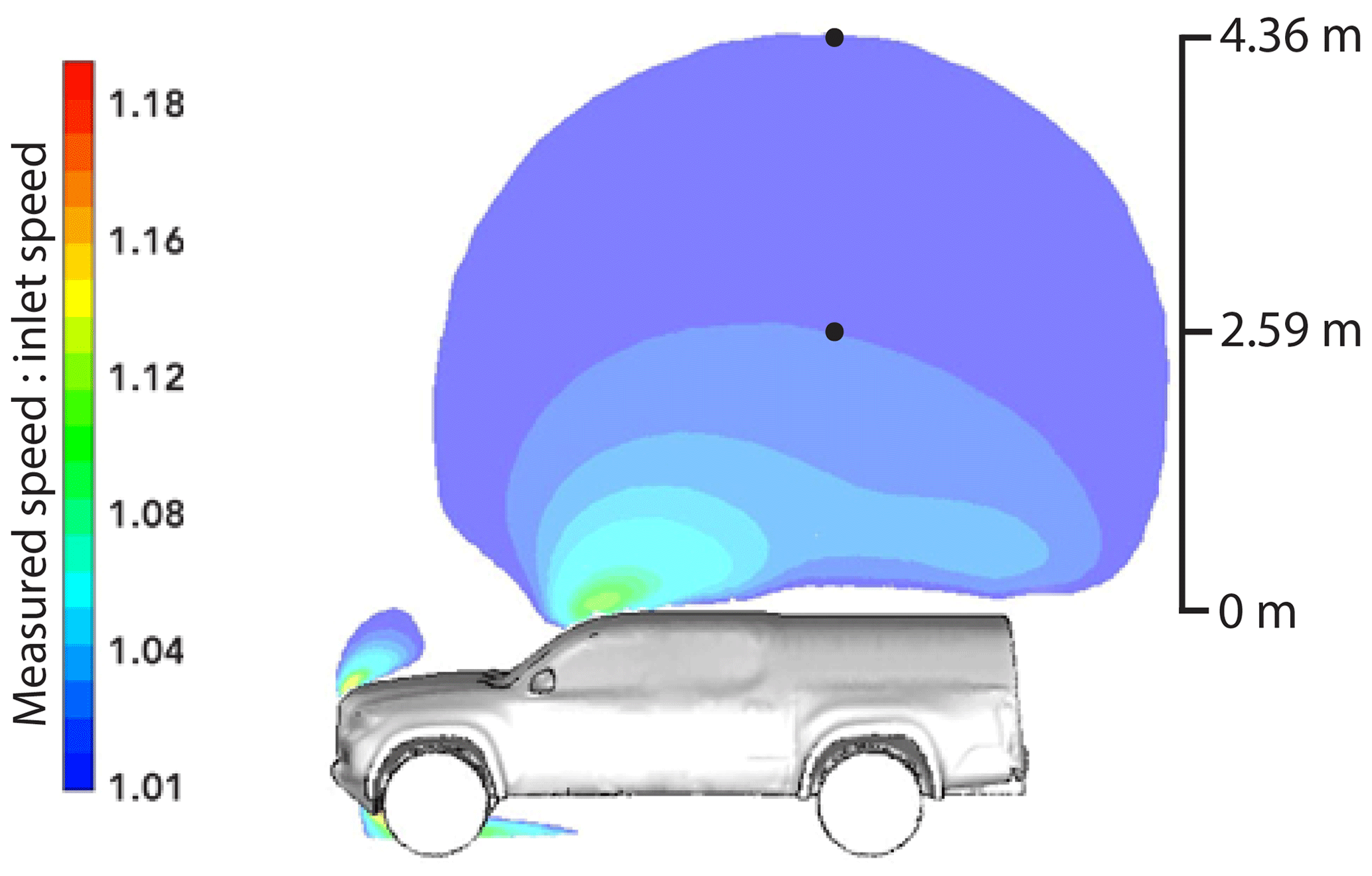
Figure 3Frontal wind velocity contour of the truck's longitudinal axis. The black dot at 2.59 m represents the anemometer height required to be subject to less than 2 % bias, and the black dot at 4.36 m represents the anemometer height required to be subject to less than 1 % bias, if mounted 30 cm behind the truck cab.

Download

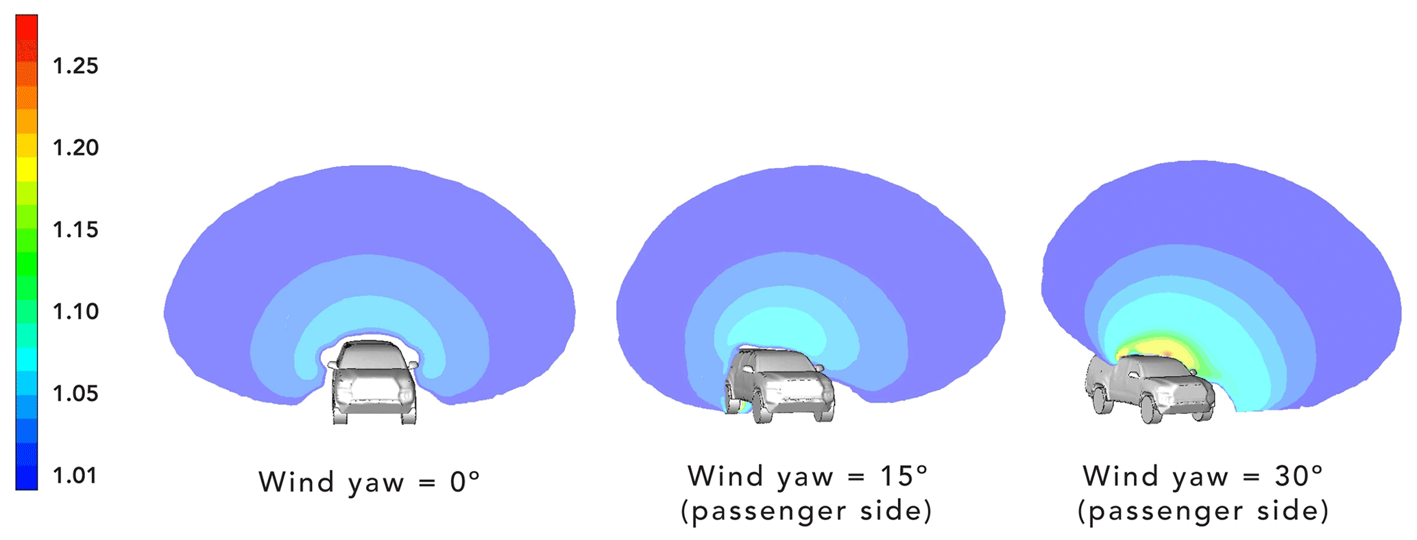
Figure 4Velocity contours of the lateral plane of the truck along the roof racks for yaw angles of 0, 15, and 30^∘. Yellow regions indicate that the wind is accelerated by 18 %.

Download

Table 2Required anemometer height for a centrally mounted anemometer to experience negligible bias.

Download Print Version | Download XLSX

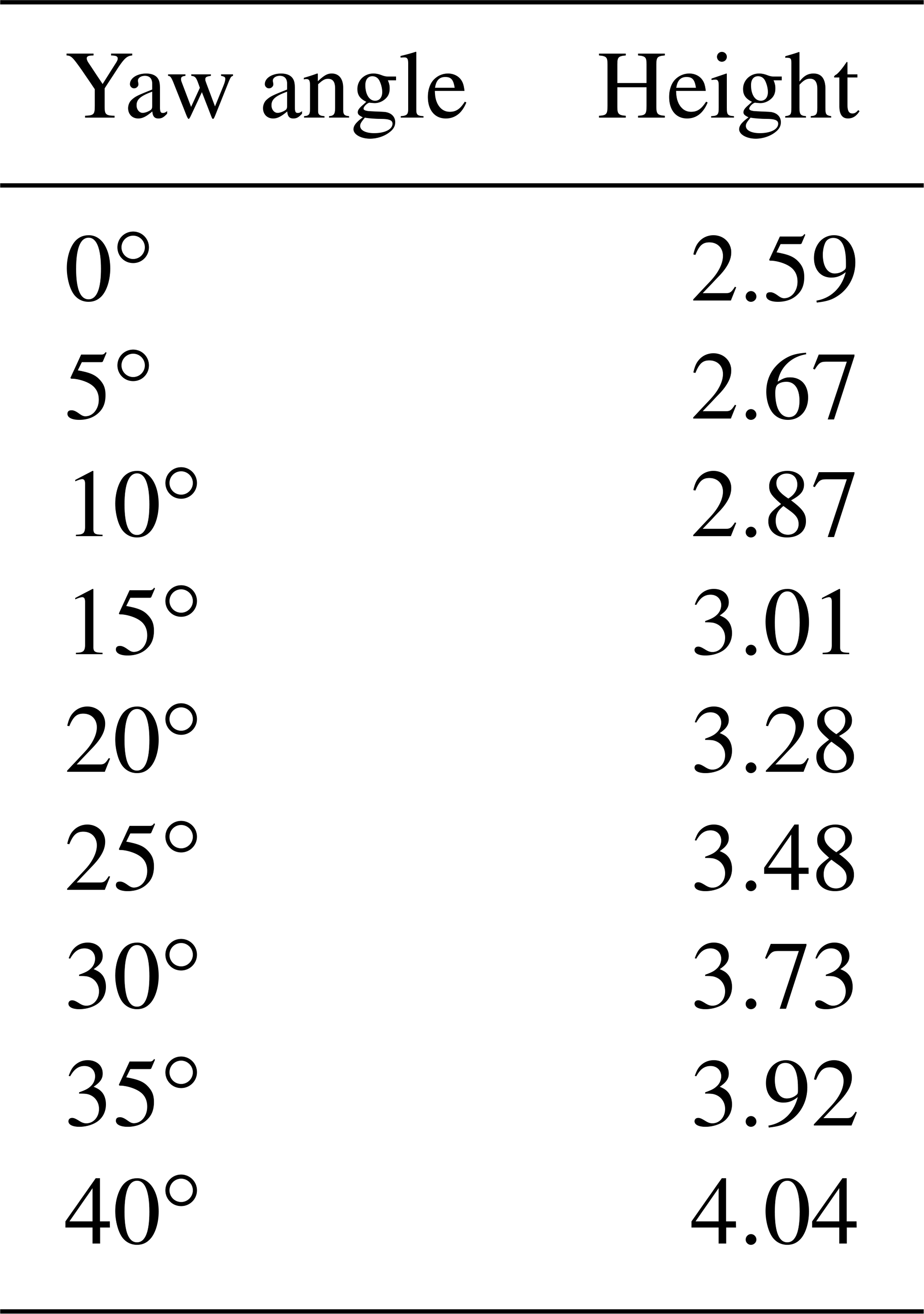
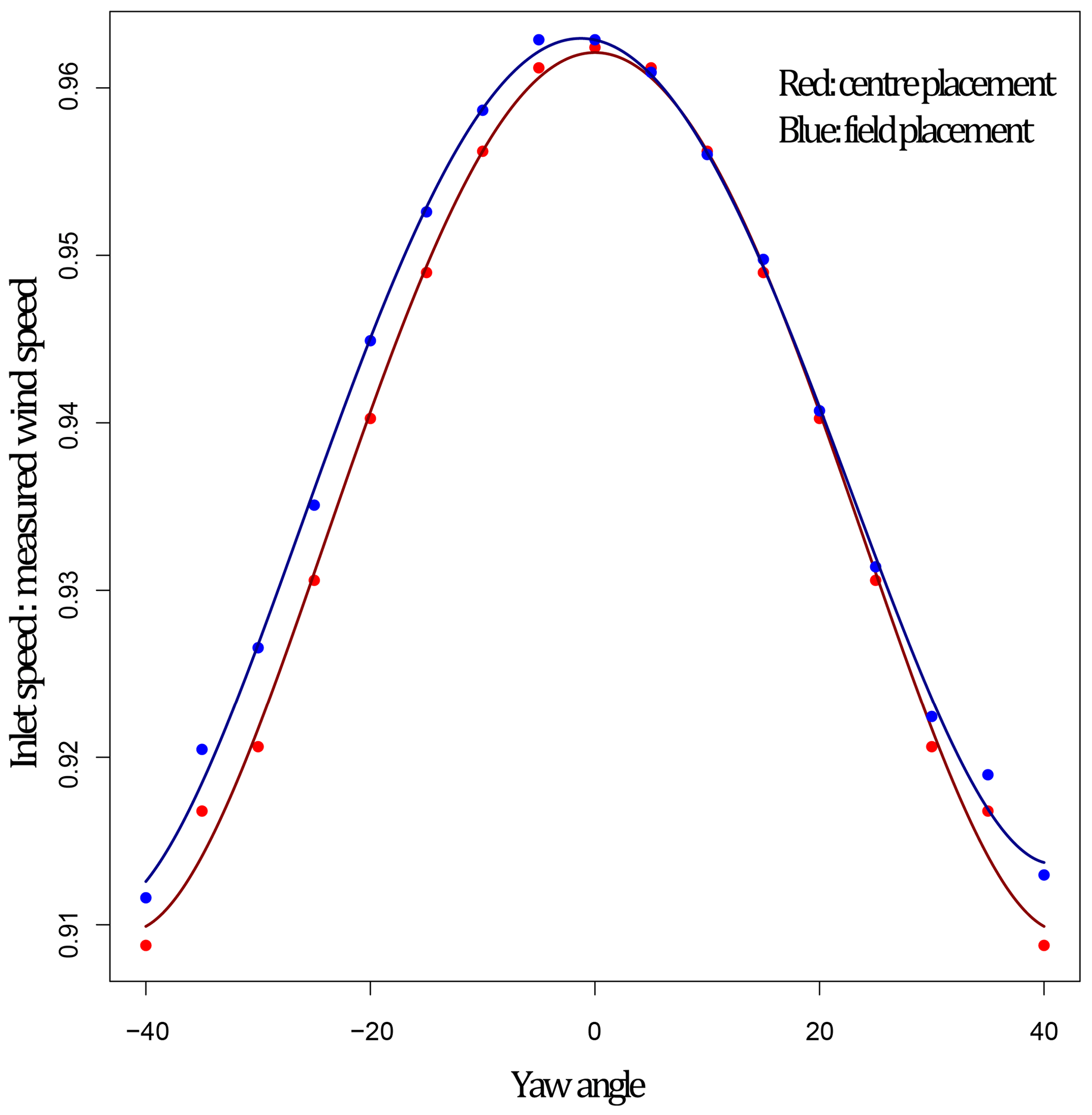
Figure 5Empirical correction factors for field placement (blue) and centred placement (red) fitted with a weighted polynomial regression.

Download

We derived aerodynamic-based correction factors to be applied to vehicle-based wind measurements from the simulation datasets. The normalized wind speed $\left(\frac{\text{measured wind speed}}{\text{inlet speed}}\right)$ at the location of an anemometer mounted in the same location as the field test was computed for each yaw angle simulation. The empirical correction factor for each yaw angle is the reciprocal of the normalized wind speed. Empirical correction factors were computed for the anemometer placement in the field trials and for an anemometer placement in the centre of the truck, above the roof racks. The correction factors for both anemometer placements were fitted with weighted polynomial regressions. Figure 5 shows the function for both placements. The centred placement provides a symmetrical function, whereas the side-mounted anemometer measures lower wind speed coming from the driver side than the passenger side. The wind coming from yaw angles over the passenger side experiences similar bias in both placements. We conclude that, by moving the anemometer to the side of the truck, we reduce the bias from wind yaw angles experienced on the driver side. Figure 5 shows that it is important that the anemometer correction function is calibrated for the anemometer placement. The polynomial pictured in Fig. 5 is multiplied by the Anemometer wind speed (A_WS) to give the corrected wind speed (WS). Equation (2) gives the side-mounted anemometer's correction function for wind direction (WD) measurements ranging $-\mathrm{40}{}^{\circ }<\mathrm{WD}<\mathrm{40}{}^{\circ }$, where the wind direction measurement is measured in the truck's coordinate system with 0^∘ facing the front of the truck. Wind speed units are in kilometres per hour (km h⁻¹) and wind direction units are in degrees.

The side-mounted anemometer placement was used in our field tests. For our field analysis, we will use Eq. (2) as an empirical correction function calibrated for anemometer placement and wind yaw angle. The empirical calibration must be applied to remove the bias of the vehicle's shape on anemometer measurements prior to correcting for the vehicle motion.

3.2 Field results

The field results provided measurements of the flow field at two locations above the truck. While the spatial resolution of the flow field was limited, the measurements were able to provide data true to the application. Vehicle-based wind measurements were acquired on separate days in predominantly north, east, south, and west winds, and with the average wind speed of the field tests ranging from 13.5 to 27.1 km h⁻¹.

Figure 6Comparison of short and tall anemometer measurements in crosswind.

Download

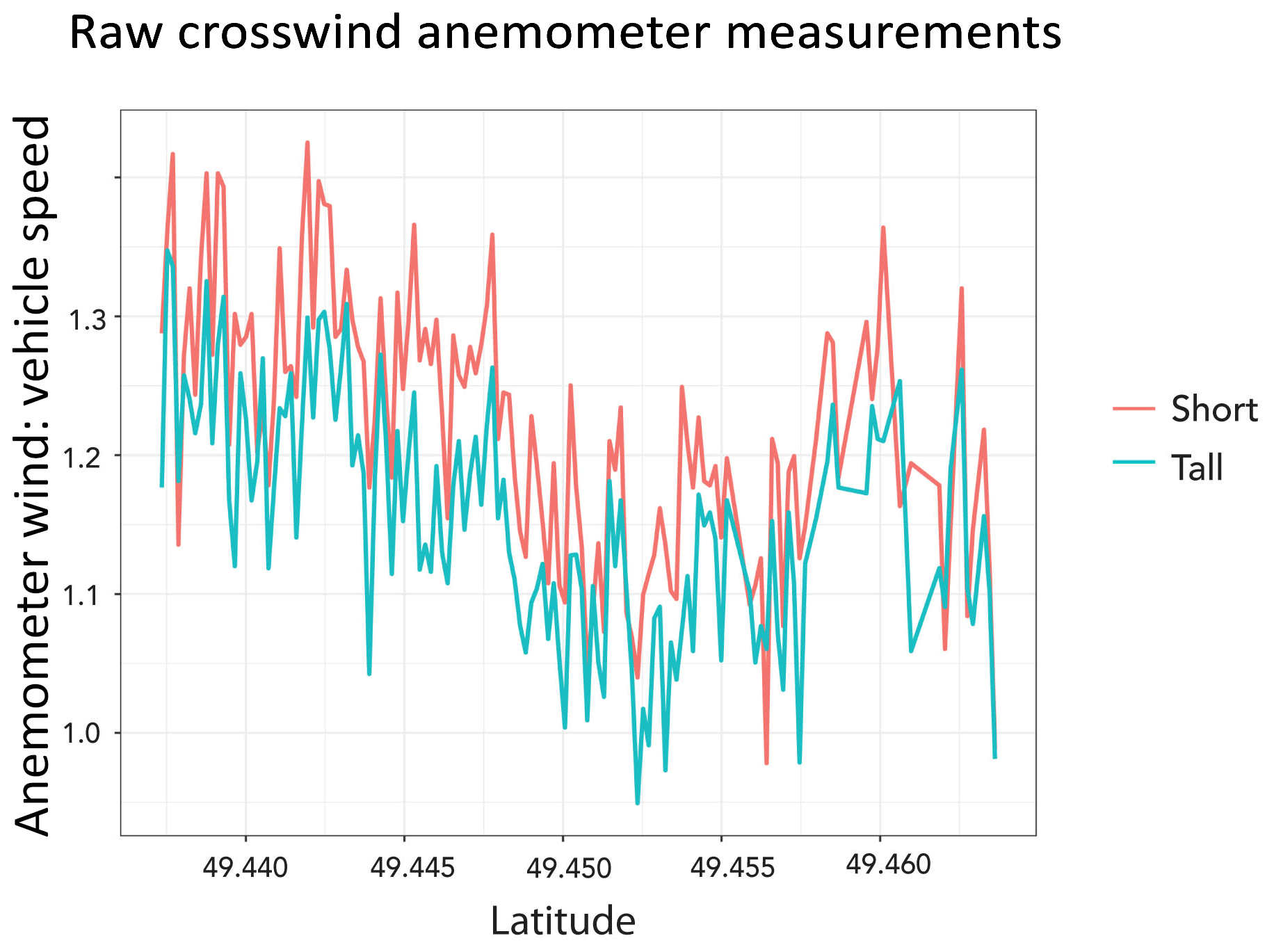
To evaluate the vertical velocity profile, we compared the measurements from the two anemometer tests. The short anemometer measured larger mean wind speeds in the head-, cross-, and tailwind directions, demonstrating that vehicle speed had a greater impact on the wind speed measurements of the short anemometer. Figure 6 shows the magnitude of the tall and short anemometer measurements when normalized by the vehicle speed. We concluded that vehicle speed had a larger effect on the short anemometer placement.

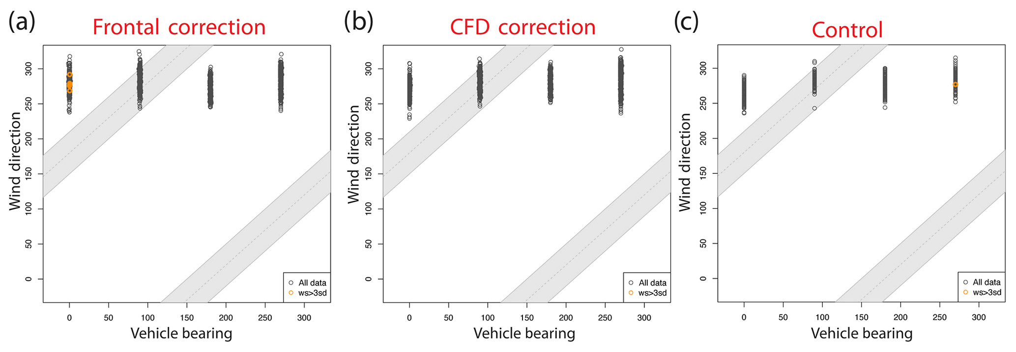
Figure 7Distribution of wind measurements across vehicle bearing with (a) frontal correction applied to mobile measurements, (b) empirical correction and frontal correction applied to mobile measurements, and (c) stationary measurements. The shaded grey bars represent measurements acquired when the vehicle was driving in tailwind conditions. The yellow circles represent wind speed measurements that are greater than 3 standard deviations away from the mean wind speed of the wind speed measurements calculated with the (a) frontal correction applied and (b) empirical correction and frontal correction applied and that are (c) specific to the stationary anemometer at each bearing.

Download

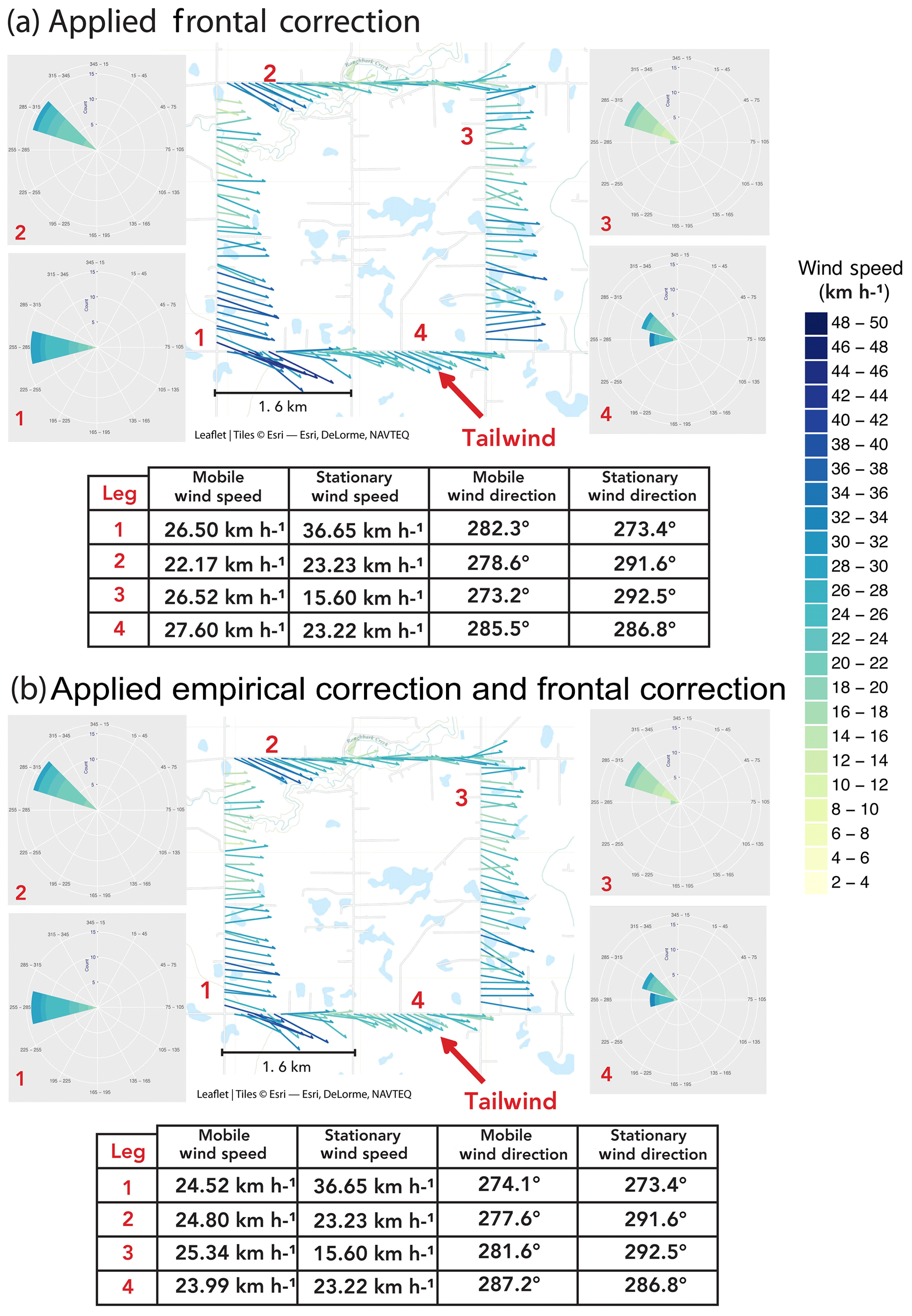
Figure 8Mobile wind vectors displayed with adjacent stationary wind roses with (a) frontal correction applied to mobile measurements, and (b) empirical correction and frontal correction applied to mobile measurements. The vehicle travelled this route in a clockwise direction. The wind roses show the direction from which the wind is blowing, and the mapped vectors indicate the direction to which the wind is blowing. The table below each plot indicates the averaged stationary and mobile wind speed and wind direction for each leg. Map data: ©Esri – Esri, DeLorme, NAVTEQ.

The field data were compared with the stationary anemometers. For our results, we present the corrected field data in two ways: (1) with the frontal wind correction, and (2) with the applied CFD empirical correction and then the frontal wind correction. We found that the application of the frontal wind correction overestimates wind speed in headwind, underestimates in tailwind, and differs in passenger side and driver side wind. Applying the CFD empirical correction reduces the overestimation in headwind and the underestimation in tailwind. It also improves the wind speed in passenger and driver side wind.

We found that applying the empirical correction reduces the wind speed measurement outliers and reduces the standard deviation of the wind direction measurements. Figure 7 shows the distribution of wind measurements across vehicle bearing. Figure 7 displays field test data with the frontal wind correction (Fig. 7a); the field data with the empirical correction applied, followed by the frontal correction (Fig. 7b); and the stationary measurements, with the vehicle bearing being that which the vehicle was driving when adjacent to that anemometer (Fig. 7c). Applying the empirical correction reduces the difference in the mean of the wind direction measurements across the four vehicle bearings. The plots outline the areas the vehicle was driving in tailwind, as we had expected more outliers to occur when driving in tailwind. The control plot shows that outliers can be expected due to the natural variability of the wind.

Figure 8 shows mapped vehicle wind vectors under the frontal (Fig. 8a) and empirical and frontal (Fig. 8b) corrections. Wind roses from the stationary anemometers on each leg are located in the corners. The measurements in the wind roses are the wind gust and average wind direction measurements reported each minute of the 14 min 60 km h⁻¹ speed test.

The mobile wind vector measurements in these plots are not averaged, and they were all taken when the vehicle was travelling within 2.5 km h⁻¹ of 60 km h⁻¹. Both plots look similar, with the largest change being the reduction of the speed of the arrows in the empirical correction plot. Figure 8 shows that applying the CFD calibration improves the agreement of the average mobile wind speed and direction measurements with the average stationary measurements in three of the four legs of the route. Observations of wind speed as measured (uncorrected for flow) show that when the truck was moving faster than 40 km h⁻¹, 72 % of raw wind direction measurements fell between −40 and 40^∘ of the front of the truck, the same as the yaw angles simulated in CFD. Field measurements were the only method of obtaining data under tailwind conditions in our study. Our CFD model was limited to a single inlet and did not have the capability to simultaneously model oncoming air from the vehicle's motion and wind blowing from behind the truck. Empirical correction factors could be derived from field experiments to provide better data for tailwind conditions. Our square experiment provided successful data for validation. The experiment could be expanded to include repetitive routes of each vehicle speed over a larger range of field days for exposure to more wind speeds. It would also be important to test on a day with little wind to identify a minimum-wind-speed-to-driving-speed ratio for field practice. The resulting vehicle anemometer dataset with corresponding stationary measurements could be used to derive empirical correction factors. The data in our study only provided one square test per speed each day, which was unable to provide data at the range of yaw angles in which CFD was successful. However, square-route driving experiments would still be a good way to obtain a field-based empirical correction function, at least for the range of wind speed and wind yaw angle conditions experienced during the test.

We found that applying the CFD empirical correction function, followed by the frontal wind correction, reduced the number of wind speed outliers found on the square route. The plotted wind vectors in Fig. 8 show that the 1 Hz mobile wind measurements experience the most variability in speed and direction when the vehicle is travelling in tailwind conditions. The empirically corrected tailwind direction measurements were in reasonable (within $\sim \mathrm{30}{}^{\circ }$) agreement with stationary direction measurements on field days with winds greater than 25 km h⁻¹ but deviated on days with lower wind speeds. When the vehicle speed is much larger than the wind speed, the vehicle creates a continuous flow field that can obstruct natural winds. The anemometer detects continuous frontal wind from the vehicle and becomes less sensitive to components of the wind coming from behind the vehicle. It is likely that a wind speed threshold for the magnitude of tailwind is detected by the mobile anemometer and that this threshold varies with vehicle speed. Additional field testing on field days with low winds is recommended to evaluate the quality of tailwind measurements, identify wind speed thresholds, and develop quality control criteria for tailwind measurements. As CFD is limited in developing an empirical correction for tailwind, additional field data are recommended to develop a correction for tailwind measurements.

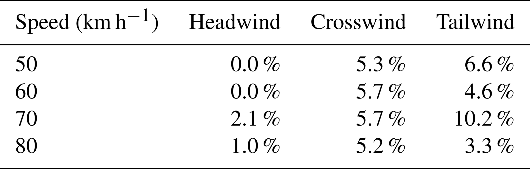
We applied the frontal wind correction to both mobile anemometers and explored the difference in the mean wind speed at each vehicle speed in head-, cross-, and tailwinds. The results are displayed in Table 3. The crosswind measurements used in this test were from the passenger side of the truck, as the post of the tall anemometer may have impacted the short anemometer measurements when the wind was coming from the driver side. The percent difference scales well across vehicle speed in head- and crosswinds. The agreement of the field measurements across vehicle speed shows that the wind speed scales linearly with vehicle speed and validates the trend in our CFD model. The measurements deviate in tailwind.

Table 3Percent difference between mean short and tall anemometer measurements across vehicle speed.

Download Print Version | Download XLSX