the Creative Commons Attribution 4.0 License.
the Creative Commons Attribution 4.0 License.
 | 20 Jan 2020
Potential for the measurement of mesosphere and lower thermosphere (MLT) wind, temperature, density and geomagnetic field with Superconducting Submillimeter-Wave Limb-Emission Sounder 2 (SMILES-2)
Satoshi Ochiai
Eric Dupuy
Richard Larsson
Huixin Liu
Naohiro Manago
Donal Murtagh
Shin-ichiro Oyama
Hideo Sagawa
Akinori Saito
Takatoshi Sakazaki
Masato Shiotani
Makoto Suzuki
Submillimeter-Wave Limb-Emission Sounder 2 (SMILES-2) is a satellite mission proposed in Japan to probe the middle and upper atmosphere (20–160 km). The main instrument is composed of 4 K cooled radiometers operating near 0.7 and 2 THz. It could measure the diurnal changes of the horizontal wind above 30 km, temperature above 20 km, ground-state atomic oxygen above 90 km and atmospheric density near the mesopause, as well as abundance of about 15 chemical species. In this study we have conducted simulations to assess the wind, temperature and density retrieval performance in the mesosphere and lower thermosphere (60–110 km) using the radiometer at 760 GHz. It contains lines of water vapor (H2O), molecular oxygen (O2) and nitric oxide (NO) that are the strongest signals measured with SMILES-2 at these altitudes. The Zeeman effect on the O2 line due to the geomagnetic field (B) is considered; otherwise, the retrieval errors would be underestimated by a factor of 2 above 90 km. The optimal configuration for the radiometer’s polarization is found to be vertical linear. Considering a retrieval vertical resolution of 2.5 km, the line-of-sight wind is retrieved with a precision of 2–5 m s−1 up to 90 km and 30 m s−1 at 110 km. Temperature and atmospheric density are retrieved with a precision better than 5 K and 7 % up to 90 km (30 K and 20 % at 110 km). Errors induced by uncertainties on the vector B are mitigated by retrieving it. The retrieval of B is described as a side-product of the mission. At high latitudes, precisions of 30–100 nT on the vertical component and 100–300 nT on the horizontal one could be obtained at 85 and 105 km (vertical resolution of 20 km). SMILES-2 could therefore provide the first measurements of B close to the electrojets' altitude, and the precision is enough to measure variations induced by solar storms in the auroral regions.


The mesosphere and lower thermosphere (MLT) is a transitional region (60–110 km) between atmospheric layers with very different characteristics, namely the stratosphere (15–60 km) and the thermosphere (90–400 km) (Smith, 2012; Shiotani et al., 2019). In the stratosphere, O3 controls the chemical and radiative processes; hence, it also regulates the temperature and the dynamics. In the thermosphere, the chemistry and the radiative balance are mainly controlled by the oxygen atoms. In this region, wind and temperature exhibit large diurnal variations and are strongly influenced by tides generated in the lower atmosphere. The thermosphere is also the region of interactions between the ionized (plasma) and neutral atmosphere.
The mean physical characteristics of the MLT (wind, temperature and density) are primarily established by energy transferred from the troposphere via small-scale gravity waves (GWs) (Fritts and Alexander, 2003; Tsuda, 2014). Hence, the MLT state deviates significantly from the radiative equilibrium, as illustrated by the occurrence of the coldest point of the Earth system (≈150 K) in the summer polar mesopause. Waves with planetary scales also contribute to the upper atmosphere climate (general circulation) through their momentum and energy transport/deposition (Forbes et al., 2006; Pancheva and Mukhtarov, 2011). In particular, tides that are mainly driven by diurnally varying diabatic heating in the troposphere and the stratosphere propagate upward, with their amplitude reaching a maximum in the MLT (Chapman and Lindzen, 1970; Sakazaki et al., 2015). Hence, the MLT plays a key role in connecting the lower and upper atmosphere and also in linking both hemispheres (Xu et al., 2009; Karlsson and Becker, 2016). Furthermore, the increase in anthropogenic CO2 is responsible for a cooling of 1–3 K decade−1 in the MLT that has been measured since the early 1990s (Beig, 2011).
The processes behind these phenomena are still not well quantified. The difficulty arises from the nonlinear interactions between the GWs, tides, planetary waves, the background wind and the electromagnetic field (Sato et al., 2018; Immel et al., 2006). The system is further complicated by the interconnections between the dynamics and highly variable chemical species, as well as the very different temporal and spatial scales of these processes. Observations of the MLT, in particular of wind, temperature and density, are therefore essential to further our understanding of this region (Smith, 2012).
Continuous measurements of temperature and wind are performed from ground-based stations using lidars (Steinbrecht et al., 2009; Baumgarten, 2010), radars (Jacobi et al., 2015; Tsutsumi et al., 2017) and, up to 70 km, millimeter radiometers (Rüfenacht et al., 2014). Density was recently monitored using meteor radars (Yi et al., 2019), but measurements remain scarce. Satellite observations of the MLT have also been performed for several decades. The missions currently in operation and capable of measuring at these altitudes are listed in Table 1. Temperature is measured with various techniques and spectral domains (Schwartz et al., 2006; Sica et al., 2008; Sheese et al., 2010; Christensen et al., 2015; Eastes et al., 2017; Englert et al., 2017), but discrepancies larger than 10 K can be found between these measurements above 80 km (García-Comas et al., 2014). Baron et al. (2013) and Shepherd (2015) described the past and current wind measurements from space. Currently only TIDI and MLS (and soon MIGHTI) are capable of measuring MLT winds but with a poor sensitivity below 80 km (Niciejewski et al., 2006; Wu et al., 2008; Englert et al., 2017), and MLS, which is equipped with a single antenna, can only measure one component of the wind vector (it was not designed for wind measurement).
Table 1Current and future satellites and instruments capable of measuring the MLT (60–110 km).
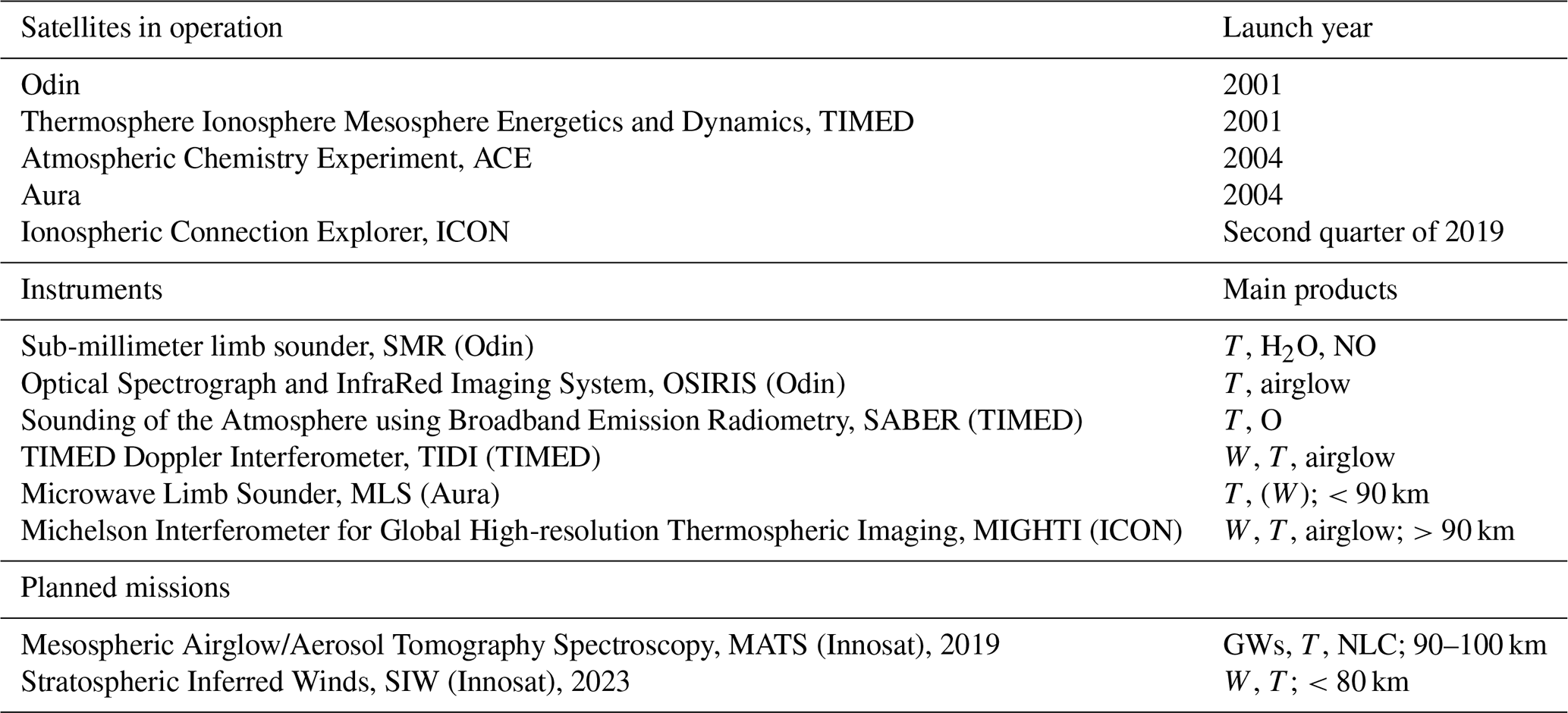
W, T and NLC denote wind, temperature and noctilucent cloud.
In the future, we clearly risk a lack of satellite observations since all the current missions (except ICON) have already exceeded their theoretical lifetime. Sweden is preparing two Innosat-based missions that are of interest for the study of the MLT (Table 1). The MATS mission aims at characterizing the 3-D structure of the GWs near 90–100 km using the oxygen A-band emission and the ultraviolet light scattered by noctilucent clouds (Gumbel et al., 2018). Information on temperature will also be retrieved. The other mission is SIW, a sub-millimeter limb sounder that will measure horizontal wind, temperature and trace gases up to about 80 km (Baron et al., 2018). The MATS and SIW missions will be operational for 2 years between 2019 and 2021 and between 2023 and 2025, respectively. Other projects have not been selected yet and remain uncertain. For example, Wu et al. (2016) proposed a THz limb sounder (TLS) to measure the atomic oxygen line at 2 THz. Such an instrument could fly together with a new version of SABER (Mlynczak and Yee, 2017). The European Space Agency (ESA) is studying a limb sounder operating between 0.8 and 4 THz for the retrieval of the abundance of chemical species such as atomic oxygen (O) or the hydroxyl radical (OH) (Gerber et al., 2013). TALIS, a limb sounder using similar spectral bands to Aura MLS, is being studied in China (Wang et al., 2019). Kaufmann et al. (2018) described a concept for a limb sounder on board a CubeSat to measure temperature with high horizontal resolution using the molecular oxygen (O2) A-band infra-red emission.
Superconducting Submillimeter-Wave Limb-Emission Sounder 2 (SMILES-2) is a middle and upper atmospheric satellite mission proposed to the Japan Aerospace Exploration Agency (JAXA) (Ochiai et al., 2017, 2019; Shiotani et al., 2019). If selected, it will be launched around 2026 on a JAXA M-class satellite. The objectives are to provide geophysical information with unprecedented precision and altitude coverage such as the temperature between 15 and 160 km, horizontal wind between 30 and 160 km, atmospheric density up to 110 km, ground state of atomic oxygen between 90 and 160 km, and more than 15 trace gases' abundance (Baron et al., 2019a, b). The proposed satellite will be equipped with two antennas for the limb measurement of horizontal winds, and three radiometers near 0.7 and 2 THz cooled at 4 K, a technology successfully tested with JEM/SMILES (Kikuchi et al., 2010). With a precessing orbit and the high receiver precision, it will be possible to retrieve diurnal variations of very weak signals, as demonstrated with JEM/SMILES (Sakazaki et al., 2013; Khosravi et al., 2013).
In this study we discuss the potential for SMILES-2 to measure the main characteristics of the neutral MLT, namely wind, temperature and atmospheric density. An essential source of information is the O2 transition at 773.8 GHz. As a magnetic dipole, O2 is subject to the Zeeman effect induced by the Earth's magnetic field (B). Special care is taken to properly include this effect in the simulations in order to correctly assess the measurement performance. Retrieval errors induced by uncertainties on B are mitigated by retrieving its three components simultaneously with other atmospheric parameters. The scientific interest of the retrieval of B is also discussed. In Sect. 2, the characteristics and principle of the observations are presented in details. Sections 3 and 4 describe the Zeeman model and the retrieval setting, respectively. The retrieval errors are discussed in Sect. 5. Finally, we summarize the results and discuss future analysis for SMILES-2.
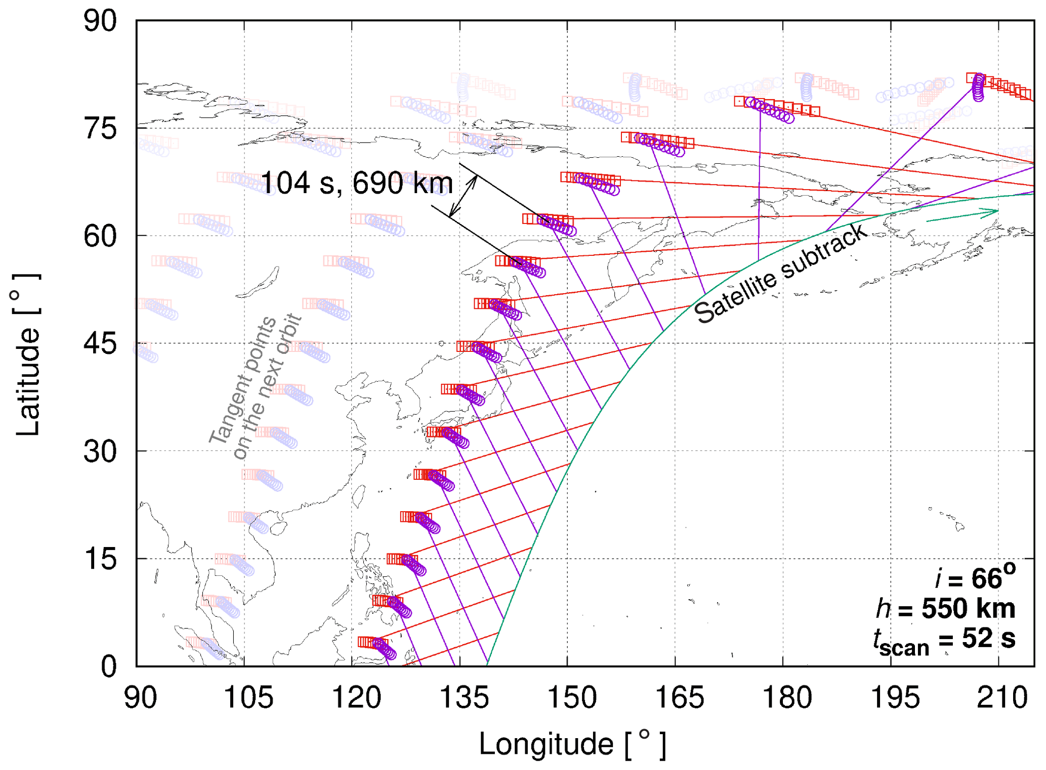
Figure 1SMILES-2 orbit over the Northern Hemisphere. The red and purple lines show the forward and aftward lines of sight (LOSs). The circles show the tangent-point footprints (Ochiai et al., 2017).
2.1 Observation method
The observation characteristics are summarized in Table 2. The atmospheric limb is scanned from about 20 to 180 km. Scans are performed alternatively with two antennas looking at perpendicular directions to each other. Both antennas can probe the same atmospheric column with a 7 min delay (Fig. 1), allowing us to derive the 2-D horizontal winds. The same method will be used for SIW and more information is given in Baron et al. (2018). The limb geometry provides a high vertical resolution of 2–3 km, and the zonal and meridional samplings at the Equator are about 20∘ (2200 km) and 6∘ (650 km), respectively.
The orbit precesses with a period of about 3 months. The satellite orientation is reversed after every half precession cycle in order to keep the solar panels properly illuminated and the radiative-cooling panels in the shadow side. The latitude coverage is between 50∘ S and 80∘ N or 80∘ S and 50∘ N depending on the satellite orientation. At low and middle latitudes, the same latitude is observed twice per orbit, with LT differences close to 12 h. Hence, gathering the observations between each maneuver allows us to piece together the complete diurnal cycle of the retrieved parameters.
Table 2SMILES2 observation characteristics.

a Calibration measurements will be performed over the upper range. b Tangent point vertical displacement during the integration time.
2.2 Spectral bands
Three spectral bands near 638, 763 GHz and 2 THz are measured simultaneously (Ochiai et al., 2018). The band at 638 GHz contains a strong stratospheric and lower mesospheric signal from ozone (O3). This band is the same as that selected for SIW and its main characteristics are described in Baron et al. (2018). Two THz bands are measured alternatively: one contains OH lines and the second one an O line (Ochiai et al., 2017; Baron et al., 2019a). The O line is used to retrieve between 90 and 160 km, the abundance of O in its ground state, wind and temperature (Baron et al., 2015, 2019b).
Table 3The 763 GHz spectral band.
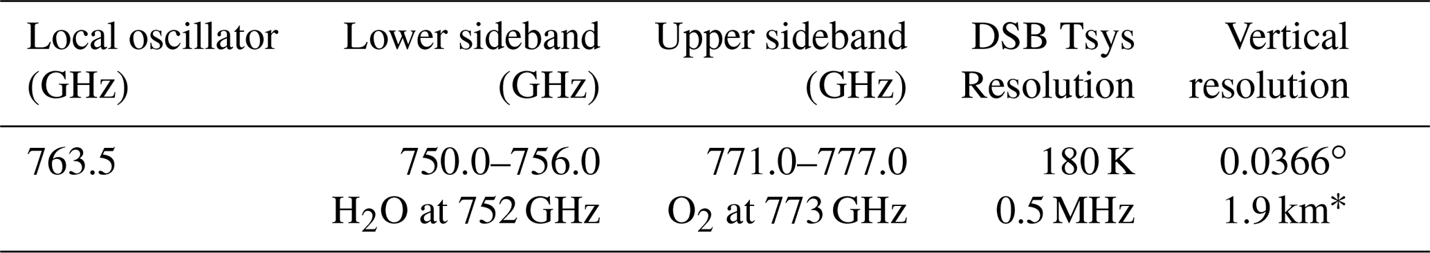
∗ Estimated for a tangent height of 80 km including the antenna field of view and the scan velocity.
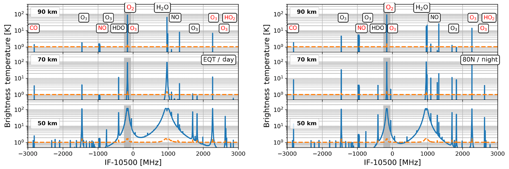
Figure 2(a) Spectra at the Equator in daytime for tangent heights of 50, 70 and 90 km. The x coordinates are the intermediate frequency (IF). The yellow dashed lines indicate the noise standard deviation (2σ). The grey area shows the frequency range of 200 MHz in which the Zeeman radiative transfer model is used (only for the upper-side band). (b) Same as (a) but for 80∘ N and nighttime winter conditions. The red labels indicate molecular lines in the upper-side band. The LO frequency is 763.5 GHz.
The 763 GHz band (Table 3) is the band considered in this study. It contains lines of water vapor (H2O) at 752.03 GHz and O2 at 773.84 GHz (Fig. 2) that provide a strong signal in the MLT. It also contains other molecular lines, weaker but still suitable for our study: nitric oxide (NO, 751.67–752.00 and 773.02–773.05 GHz), O3 (754.46 and 776.66 GHz) and carbon monoxide isotopologue (13CO) at 771.183 GHz. The bands have changed compared to those originally described by Ochiai et al. (2017), a change motivated to reduce the power consumption. In the new setting, the CO line is about 50 times weaker than that previously selected.
2.3 Qualitative description of the information content
Most of the lines in the spectral bands are emitted by chemical species in their ground state under local thermodynamic equilibrium. The molecular abundance and the temperature are retrieved from the amplitude of the lines. Their Doppler shift (2.5 kHz for 1 m s−1) is used to retrieve the line-of-sight (LOS) wind. The atmospheric density is derived from the O2 abundance considering that the volume mixing ratio of O2 is well known below 110 km (Schwartz et al., 2006).
Above about 70 km, the lines are broadened by the random molecular motions, i.e., Doppler broadening, and they do not carry direct information on the pressure (Appendix A). Consequently, the density of the molecule can be retrieved and not the volume-mixing ratio (VMR) as in the lower altitudes.
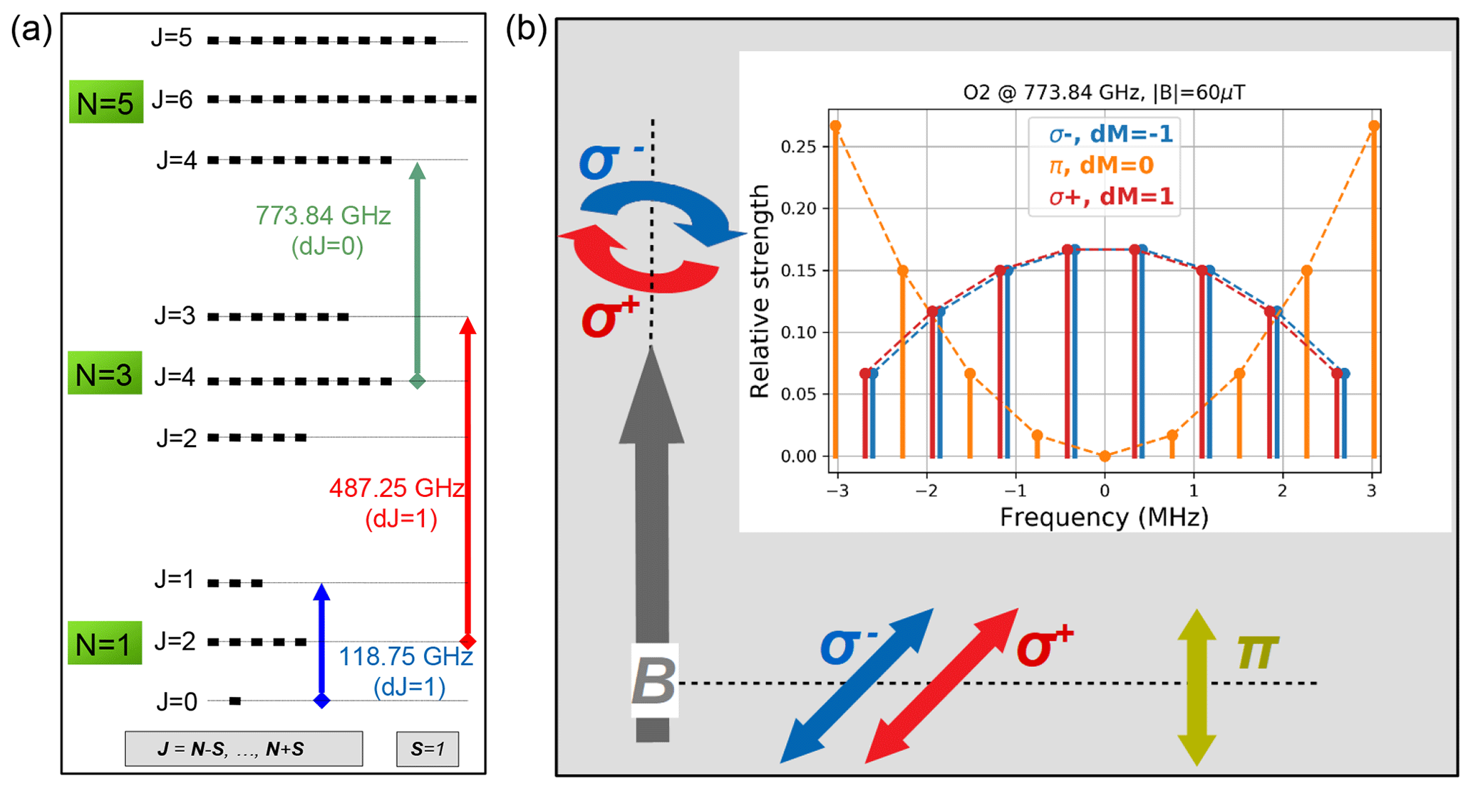
Figure 3(a) Energy levels of the O2 transitions measured with MLS at 119 GHz (Schwartz et al., 2006), SMR at 487 GHz (Larsson et al., 2014) and SMILES-2. The degenerated energy levels () are indicated with black horizontal strokes. (b) Strength and polarization of the Zeeman components of the line chosen for SMILES-2. The components' frequency is computed for a magnetic field of 60 µT (0.6 Gs). The representation of the polarization states is adapted from Fig. 3.1 in Landi Degl'Innocenti and Landolfi (2004). The dashed lines represent perpendicular and parallel LOSs with respect to B (grey thick arrow).
Molecular oxygen is a magnetic dipole that interacts with B. It is subject to the Zeeman effect (Lenoir, 1968) and the selected spectroscopic transition is split into σ± and π components with different polarization states depending on the LOS orientation (Fig. 3). The frequency separation of the spectral components is proportional to the amplitude of B.
2.4 LOS altitude
In this study, we consider LOS tangent heights between 60 and 110 km. They are provided as input for the inversion algorithm; therefore they must be known before inverting the spectra. Height registration for a complete scan is calculated differently in the lower part of the scan and in the range of interest (between ∼20 and 60 and between 60 and 110 km, respectively).
Between 20 and 60 km, an approach similar to that used for Aura MLS (Schwartz et al., 2006) can be used. The LOS tangent pressure and atmospheric temperature would be retrieved simultaneously from the O2 line near 763 GHz and from O3 lines in the 638 GHz band. The height of the pressure levels would then be derived from the hydrostatic equilibrium equation. The resulting precisions are estimated to be better than 1 % and 75 m for the LOS tangent pressure and height, respectively (Baron et al., 2019b).
In the altitude range of interest (>60 km), the LOS tangent heights are inferred from the extrapolation of those calculated previously for the lower altitudes and attitude data from the star-trackers and GPS on board the satellite. Based on JEM/SMILES results, the expected precision on the retrieved LOS tangent heights will be 100 m or better (Ochiai et al., 2013).
The Zeeman effect on atmospheric molecular-oxygen lines has been extensively studied (Lenoir, 1968; Pardo et al., 1995; Schwartz et al., 2006; Larsson et al., 2014; Navas-Guzmán et al., 2015). In this study, we describe the polarized radiance with Stokes vectors as in Landi Degl'Innocenti and Landolfi (2004) (e.g., Eq. 1.32), Larsson et al. (2014) and Steiner et al. (2016). The magnetic field characteristics (amplitude and orientation angles with respect to the LOS) are defined at the LOS tangent height (Fig. 4) and are assumed to be constant over the LOS. This approximation is the same as that used by Yee et al. (2017), and it is justified since most of the retrieved information comes from a thin altitude range around the tangent point.
3.1 Absorption matrix
The interaction between the radiation and the atmosphere are described by the 4×4 absorption matrix K:
where I is the identity matrix, ka is the scalar absorption coefficient and Ko is a matrix with off-diagonal components:
The scalar absorption coefficient is computed using a line-by-line model and the Zeeman effect is only applied on the O2 transition:
where ν is the frequency, z is the altitude, t denotes a spectroscopic transition of the species M that is not affected by the geomagnetic field, nM () is the number density of M (O2), St is the line strength, F is the Voigt function (Schreier et al., 2014; Larsson et al., 2014) and Γt,z represents the parameters related to the linewidth (Appendix A). The angle θ is the inclination angle of the magnetic field with respect to the LOS (Fig. 4a).
Table 4Zeeman transitions characteristics for the O2 line at 773.84 GHz ( and =1). The relative strengths are normalized such as (Table 3.1 in Landi Degl'Innocenti and Landolfi, 2004). The frequency shift factors βm are from Eq. (5).
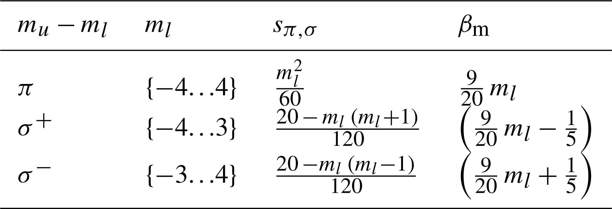
The frequencies νσ,π (Hz) are those of the Zeeman components (Fig. 3). They are dependent on the magnetic field (Larsson et al., 2014):
where gs=2.002064, μb is the Bohr magneton ( J T−1), hp is the Planck constant ( m2 kg s−1) and
Here, the lower scripts u and l denote the upper and lower levels of the transition, respectively, and N, J, S and m are quantum numbers associated with the angular momentum, the spin, the total momentum N+S and the projection of J on the B axis.
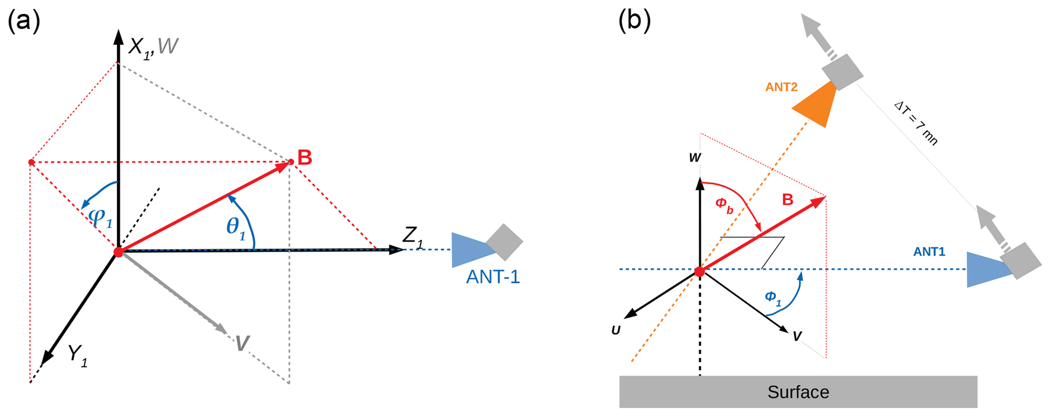
Figure 4(a) Cartesian and spherical frames used for the radiative transfer calculation. The x and z axes are along the vertical axis (W) and the LOS, respectively. (b) Frame for describing the observation of the same air mass from the forward (ANT1) and aftward (ANT2) antennas. The background geomagnetic field (B) is at first approximation in the meridional plane.
The coefficients of Ko are derived from Landi Degl'Innocenti and Landolfi (2004) (Eq. 5.36):
The parameters u′, v′ and q′ are computed by replacing the term F with F′, the dispersive part of the complex Voigt function (see Appendix A and Schreier et al., 2014).
3.2 Radiative transfer
The LOS is divided in narrow ranges of size ds (typically 5 km long) in which the atmospheric parameters are considered constant. The change of the polarized radiance passing through an homogeneous range is derived from a matrix equation which is similar to the scalar radiative transfer one used for a nonpolarized radiation (Semel and López, 1999):
where ba(s) is the Stokes vector at the position s on the LOS (the frequency dependence is omitted), “⋅” is the matrix multiplication operator, describes the nonpolarized source function between s and s+ds, P(s) is the Planck function, and is 4×4 evolution operator matrix defined as follows:
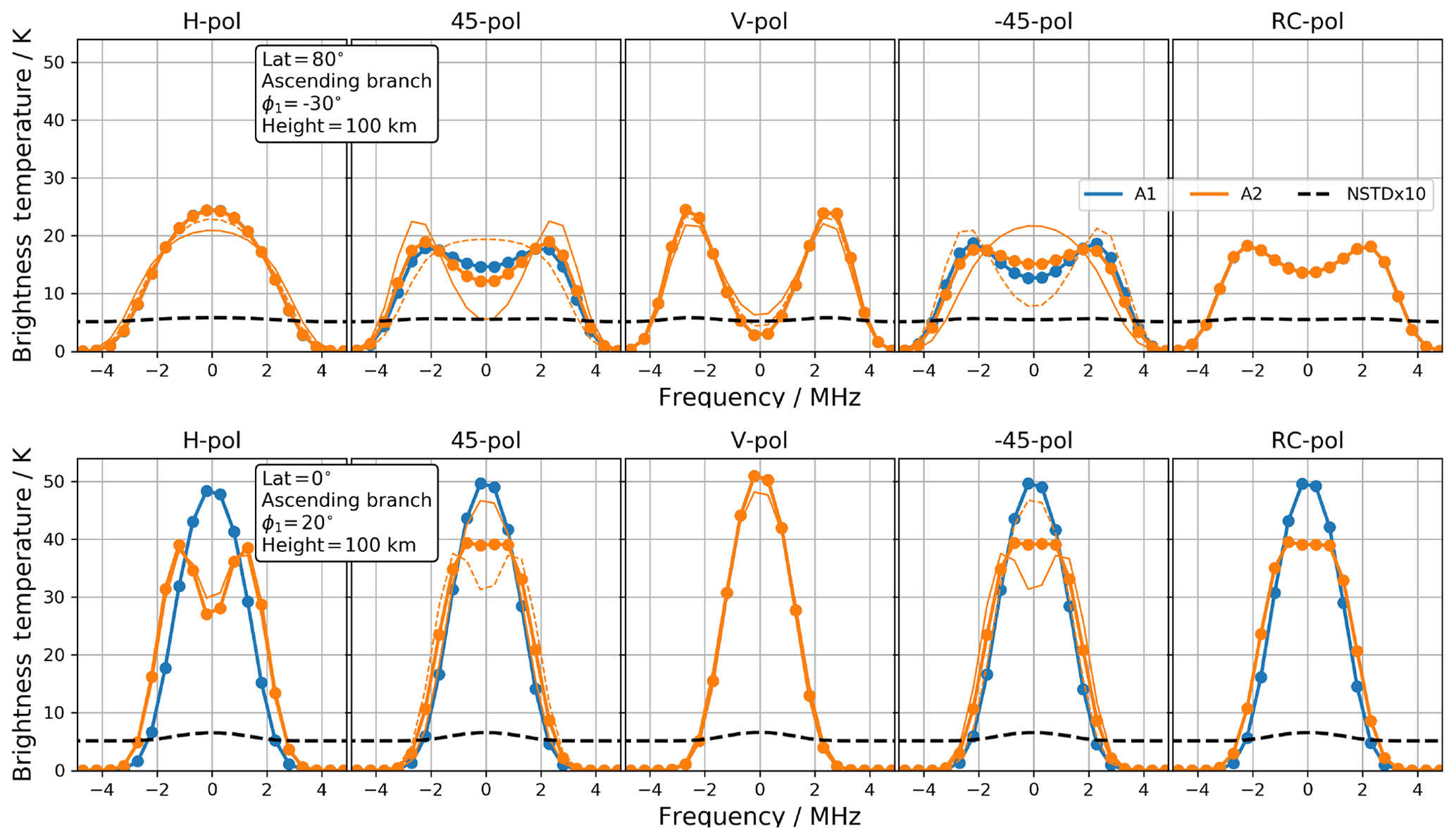
Figure 5Upper panels: O2 lines simulated for antenna-1 (blue) and antenna-2 (yellow) at 80∘ N over the ascending orbit. Panels from left to right show the results for a detector with horizontal, , vertical, and right-circular polarization. The dashed and full yellow thin lines are spectra calculated with an angular tilt of the antenna-2 detector of −20 and . The black dashed lines are the measurement noise STD × 10 for antenna-1. Lower panels: same as upper panels but for the Equator.
The integration over the LOS is performed by applying the scalar equation given by Urban et al. (2004) to Stokes parameters:
where ba(sat) is the Stokes vector representing the radiation state at the antenna position, i is the index of the level at si (i=0 for the tangent point) and N is the number of levels above the tangent point. The cosmic background radiation is neglected. We use the relationship with (the two matrices on the right-hand side of the equality do not commute).
4.1 Measured radiance
The measured radiance for antenna a (a=1 or 2) at the elevation angle θ and the IF ν is as follows:
where ya,u and ya,l are the atmospheric specific intensities in the upper and lower sidebands around the local oscillator frequency νLO, Rθ,ν represents the antenna and spectrometer functions, and ![]() is the convolution operator (Baron et al., 2018). A simple case with a constant upper and lower sideband ratio is considered.
The Zeeman model is only used within a
bandwidth of 200 MHz encompassing the O2 line (upper sideband). Outside this range, the nonpolarized radiative transfer model described in Baron et al. (2018) is used.
In order to transform the Stokes vector (Eq. 9) to the specific intensity associated with the radiometer's polarization, we first rotate the vector from the atmospheric frame to the detector frame as follows:
is the convolution operator (Baron et al., 2018). A simple case with a constant upper and lower sideband ratio is considered.
The Zeeman model is only used within a
bandwidth of 200 MHz encompassing the O2 line (upper sideband). Outside this range, the nonpolarized radiative transfer model described in Baron et al. (2018) is used.
In order to transform the Stokes vector (Eq. 9) to the specific intensity associated with the radiometer's polarization, we first rotate the vector from the atmospheric frame to the detector frame as follows:
where bd is the Stokes vector in the instrument frame and Mr(αd) is the Mueller matrix for a rotation αd:
The specific intensity y corresponding to the detector polarization is
where bd[n] is the nth component of the Stokes vector and (m,n) is , (1,1), , (1,2), and (1,3) for horizontal, vertical, +45, , right and left circular polarizations, respectively.
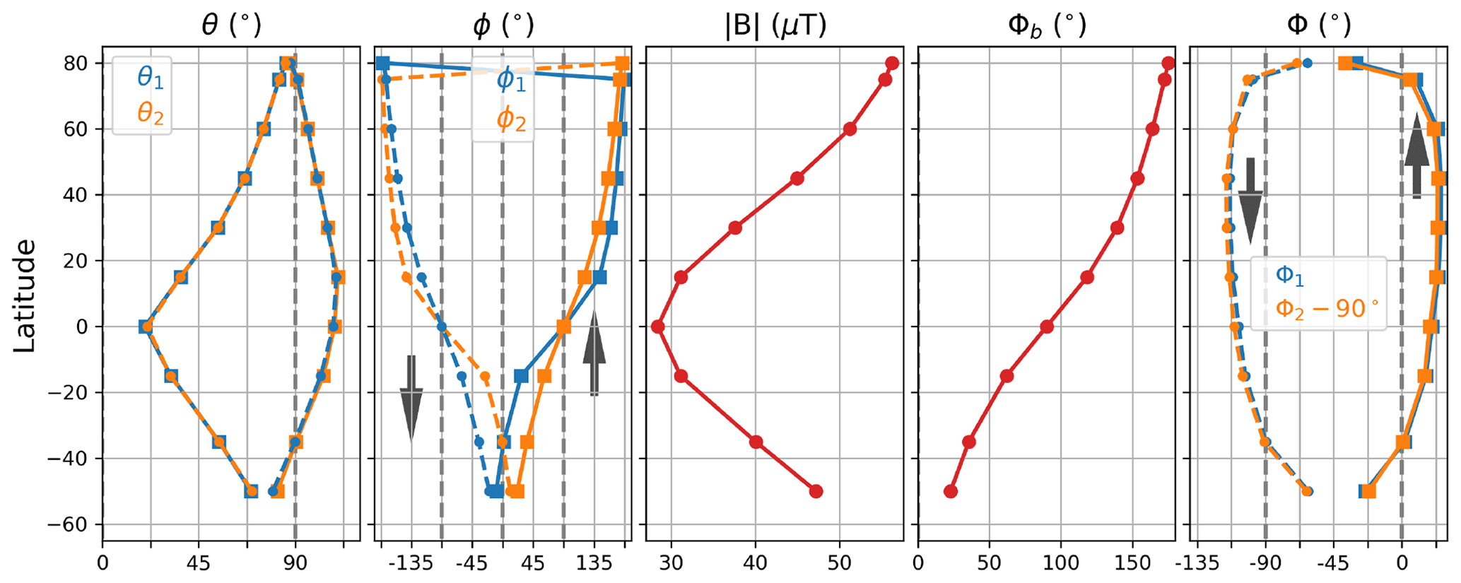
Figure 6Magnetic field (θ1,2, ϕ1,2, and Φb) and LOS (Φ1,2) parameters (Fig. 4) with respect to latitudes. The blue (yellow) lines are for ANT1 (ANT2) data. The circle–dashed (square–full) lines are data on the descending (ascending) orbit branch. The grey arrows in panels 2 and 5 indicate the direction of the satellite motion.
Figure 5 shows simulated spectra of the O2 line over the Equator and at 80∘ N when the satellite is moving toward north (ascending orbit branch). The tangent height is 100 km and the atmospheric conditions are representative of the Northern Hemisphere in wintertime (Baron et al., 2018). The magnetic field characteristics are zonal means inferred from a quiet solar day (Fig. 6). Spectra are shown for different radiometer's polarizations. Over the Equator, B is along the meridional direction and clear differences are seen between the radiances measured with both antennas, except if the detector has a vertical polarization. In that case, the radiometer detects only the σ± lines independently of the LOS orientation. The antenna-1 spectrum measured with a radiometer with a horizontal polarization is sensitive to the π components which gives the visible double line shape. A receiver with a right-circular polarization measures mainly the σ+ components since the antenna-1 is nearly aligned with the magnetic field ( in Fig. 6). The spectrum looks like a single line with a frequency shift of kHz (Eq. 4), equivalent to a LOS wind of 8 m s−1.
Over the polar region, the spectra measured by both antennas are very similar since the vector B is almost vertical and perpendicular to both LOSs (Fig. 6). Only the Zeeman components π are detected with the receiver with vertical polarization, while the horizontally polarized one detects σ± components (Fig. 3).
4.2 Retrieval setting
The geomagnetic field may exhibit rapid temporal and spatial variations that can be as large as hundreds of nanoteslas (Doumbia et al., 2007; Yee et al., 2017). Such variations will be difficult to take into account when processing the data and may lead to retrieval errors with the same magnitude as those induced by the measurement noise.
Such errors are mitigated by retrieving the three components of B simultaneously with other atmospheric parameters. It is done by using the scans of the same atmospheric column measured with the two antennas (Fig. 4). The measurement vector y is defined accordingly as follows:
where the superscripts a1 and a2 denote that the parameters are associated with the antennas 1 and 2, respectively. The vector x describing the retrieved parameters contains the profiles of the chemical species having the most significant features in the MLT spectra, namely O2, H2O, O3, NO and HDO (Fig. 2). It also includes the profiles of temperature T, LOS winds (LW) and the three components of B. It is defined as follows:
where xBw, xBu and xBv are the profiles of the vertical, zonal and meridional components of B. The abundance and temperature profiles are retrieved for each antenna in order to account for differences between both scan locations. This is a similar approach to that used by Hagen et al. (2018) for the measurement of winds with the ground-based radiometer WIRA.
The retrieval error induced by the measurement noise is (Rodgers, 2000)
where is the Jacobian matrix of the retrieved parameters x and U is a diagonal matrix to ensure a stable inversion but with values large enough to allow us to neglect its effects in the altitude range where the retrievals are relevant (Baron et al., 2018). The matrix Sy is the diagonal covariance matrix associated with the measurement noise:
and is the noise induced variance on the ith component of the measurement vector y, Tsys is the system temperature (Table 3), δν is the frequency resolution (0.5 MHz) and δt is the spectrum integration time (0.25 s).
The radiative transfer model computes the Jacobian with respect to antenna-i frame ( in Fig. 4a). The matrix KB is then computed in the atmospheric frame (Fig. 4):
where denote the atmospheric frame axes, and
where Φi is the angle between the antenna-i LOS and the meridional direction (Fig. 4a).
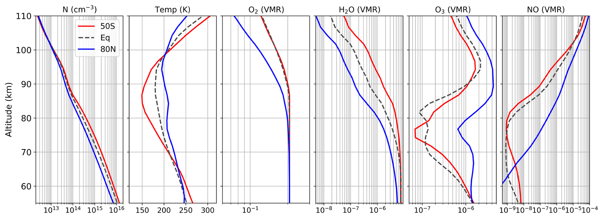
Figure 7Vertical profiles of atmospheric number density, temperature and VMRs of O2, H2O, O3 and NO. They are representative of a Northern Hemisphere winter period (DJF), during daytime at 50∘ S and the Equator (dashed-grey and red lines, respectively), and polar night at 80∘ N (blue lines).
Figure 8 shows the retrieval errors on the atmospheric density, temperature, LOS wind and the main chemical species at three latitudes (50∘ S, Equator, 80∘ N). For the instrumental setting, we considered a radiometer with a linear vertical polarization and the forward-looking antenna (antenna-1). The vertical resolution of the retrieved profiles is 2.5 km for the main parameters (temperature, LOS wind, H2O and O3), 5 km for NO and 20 km for the components of B. Errors are computed for the same winter (DJF) climatology described in the previous section. The corresponding atmospheric state includes a stable polar vortex and does not show any NO enhancement due to energetic particle precipitation. The results at the Equator and the Southern Hemisphere (SH) mid-latitudes (50∘ S) are for daytime conditions, while the Northern Hemisphere (NH) results at 80∘ N are representative of the polar night. We did not find significant differences between daytime and nighttime except for the relative error in O3 retrieval, which is photo-dissociated between 60 and 80 km.
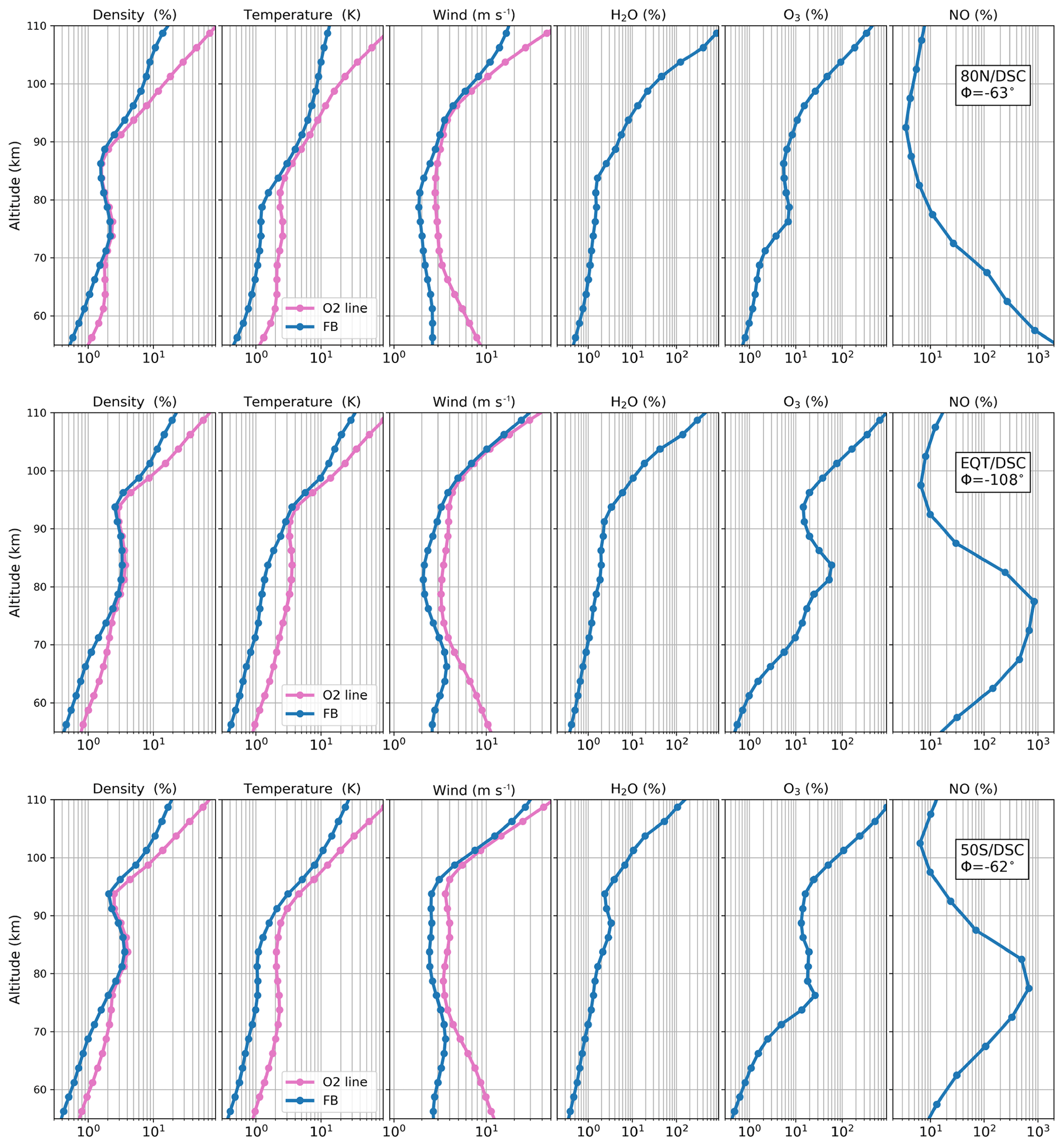
Figure 8Errors on atmospheric density, temperature, LOS wind, H2O, O3 and NO profiles. Only errors induced by the measurement noise are shown, for profiles retrieved from the antenna-1 signal using a radiometer with linear vertical polarization. The pink and blue curves show the results for the 200 MHz narrow band around the O2 line and for the full bandwidth, respectively. (a) Results at 80∘ N (polar night). (b, c) Results for daytime conditions at the Equator (b) and 50∘ S (c). The vertical resolution for the retrievals is set to 2.5 km for all profiles, except for NO, for which 5 km is used.
The results for the full band are compared with those computed for the inversion of a 200 MHz band containing only the O2 line. The purpose is to isolate and characterize the contribution of the H2O, O3 and NO spectral lines to the retrieval of MLT parameters, in terms of altitude range and impact on the retrieval errors. Latitudinal differences are induced by the mean meridional circulation (from the summer pole to the winter pole). In the winter hemisphere, it is responsible for an increase in NO and a decrease in H2O, especially over the polar region. The largest sensitivity to NO is found in the upper part of the MLT. The precision is better than 10 % above 95 km at 50∘ S and above 78 km over the winter polar region (NH in this study). A precision of 10 % or better is achieved above 95 km at 50∘ S and 78 km in the winter polar region. The sensitivity to H2O decreases with increasing altitude, more sharply above 90 km. The precision is better than 1 % up to 75 km in the SH and 65 km in the NH polar region.
The relative error in O3 retrieval is ∼1 % around 60 km and strongly increases with increasing altitude and outside of the polar night, because of the daytime photo-dissociation of O3.

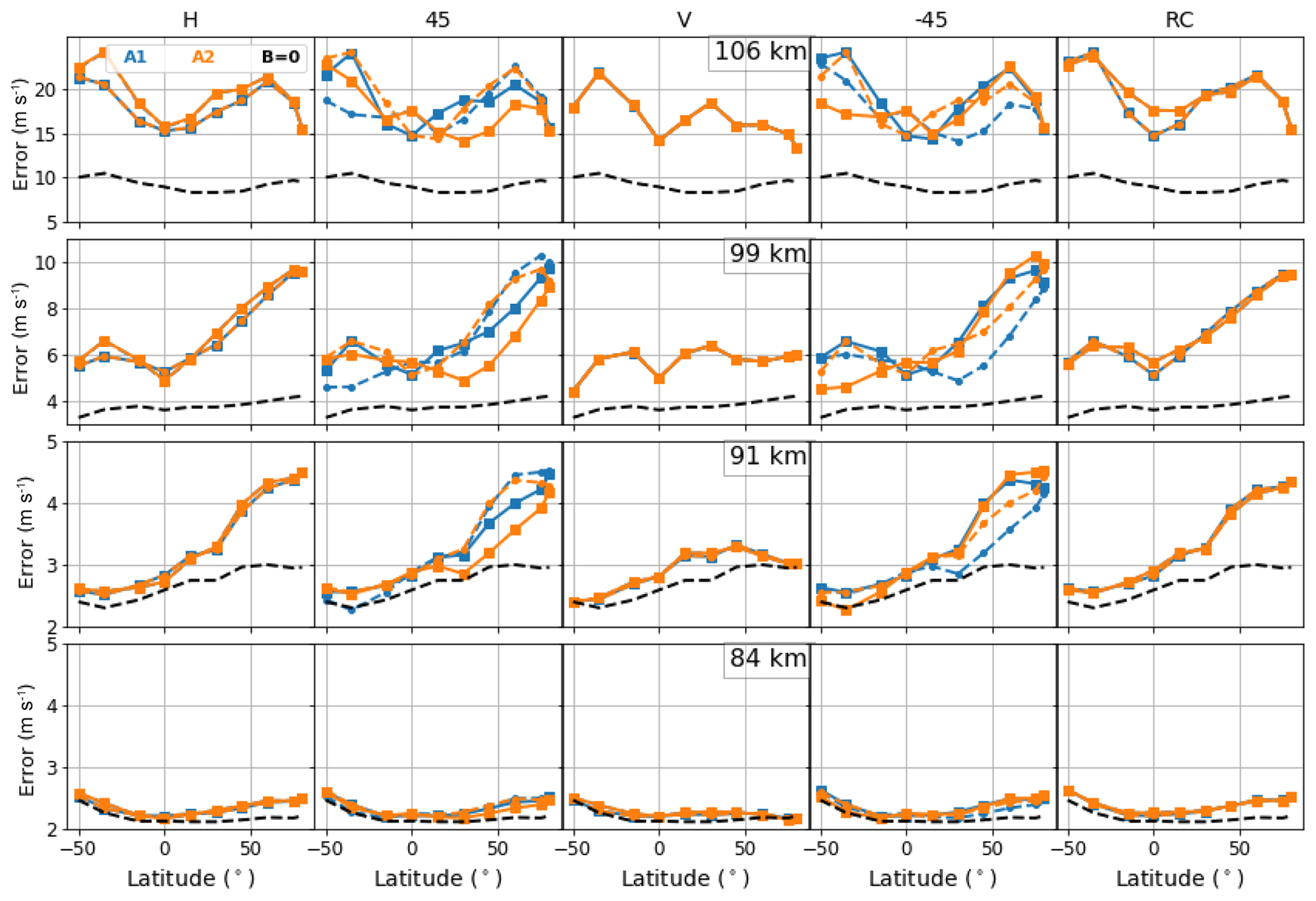
Figure 9Retrieval errors on the temperature profile induced by the measurement noise, for a radiometer with horizontal (H), 45∘ (45), vertical (V) and (−45) linear polarizations, and right circular (RC) polarization. The colored dashed lines are results for the descending orbit branch while the full lines ones are those for the ascending branch. The blue (yellow) lines show the results for antenna-1 (antenna-2). The black dashed lines show the errors that occur if the Zeeman effect is not considered. Vertical resolution of the retrieved profiles is 2.5 km.
5.1 Atmospheric density, temperature and LOS wind
The achieved precision of the atmospheric density (or O2) profile is better than 5 % up to about 95 km at all latitudes. Above 90 km, the signal intensity drops significantly and errors quickly increase, up to 20 % at 110 km. Outside of the 70–90 km range, there are significant differences between the error profiles calculated for the full- and narrow-band inversions. This shows that spectral lines from other molecular species also have an impact on the O2 retrievals. This impact probably occurs through the temperature retrieval. For instance, over the winter polar region, the strong NO signal significantly improves the temperature retrievals and thus indirectly improves the O2 abundance retrieval. Similarly, including H2O and O3 lines leads to an improvement of the O2 retrieval quality below 70 km.
For all latitudes, the temperature retrieval error is better than 5 K below 90 km and 30 K at 110 km. The O2 line is the main source of information on the temperature near 90 km.
The LOS wind, a key product for SMILES-2, is retrieved with a precision of 2–4 m s−1 up to 90 km. Above this altitude, the retrieval errors strongly increase, up to 20 m s−1 or more at 110 km. The O2 line is the main source of information on the LOS wind above 70 km. Over the polar region and above 100 km, spectral lines of NO contribute significantly to the LOS wind retrievals.
Figures 9 and 10 show the achieved retrieval precisions for temperature and LOS wind, at altitudes between 80 and 110 km and for different polarization settings. Results are shown within the latitude range 50∘ S–80∘ N, for both antennas and for both the ascending and descending orbit branches. The results obtained with B=0 are also presented.
For atmospheric temperature and below 90 km, the Zeeman effect has a negligible impact on the retrieval errors. Differences can be seen only at high latitudes, where the decrease in the H2O abundance explains the larger impact of the O2 line on the retrieval. In terms of LOS wind retrieval, the Zeeman effect is negligible below 80 km. Above 90 km, the approximation B=0 leads to a significant underestimation of the retrieval errors, with differences of up to a factor of 2. This clearly shows that the retrieval errors depend on the radiometer polarization, the LOS orientation and on the characteristics of the magnetic field.
The best overall precision is found for a radiometer with a linear vertical polarization. For instance, at NH high latitudes, the LOS wind retrieval error at 99 km is 6 m s−1 using a linear vertical polarization, but degrades to about 10 m s−1 for other polarization settings. Furthermore, using the linear vertical polarization yields homogeneous results for different observation geometries: we could not find significant differences between ascending and descending orbits or between the two antennas.
5.2 Geomagnetic field
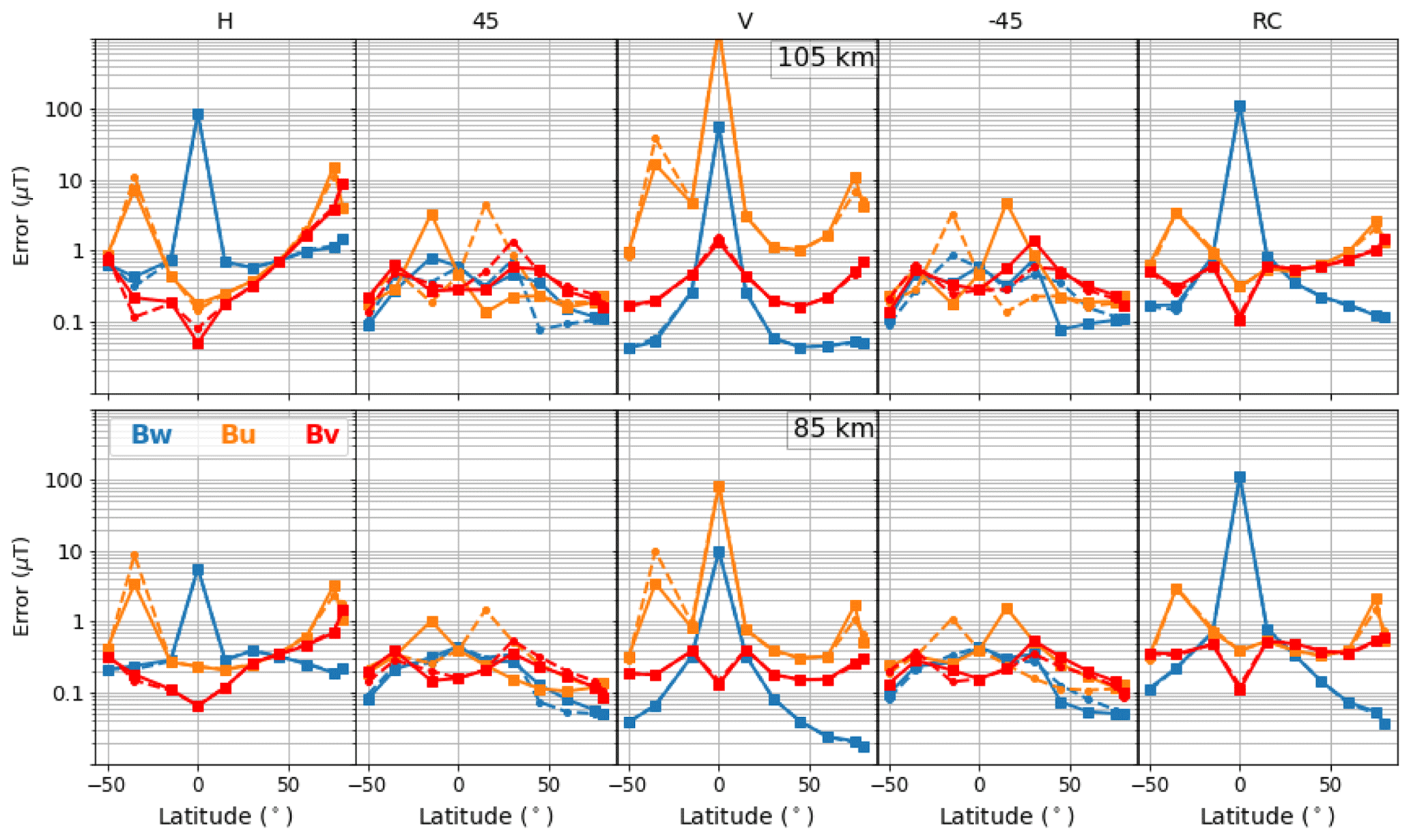
Figure 11 shows the retrieval errors on the three components of B at 85 km and 105 km (vertical resolution of 20 km). The results strongly depend on the radiometer's polarization. Best performance is achieved with a linear polarization. Errors are clearly smaller when the retrieved component is aligned with the background magnetic field: the error on Bv is smallest at the Equator where B is horizontal and in the meridional plane, and the error on Bw minimizes at high latitudes where B is nearly vertical. The best sensitivity is found at 85 km where the precision is better than 400 nT for all components and at all latitudes, except for the zonal component (Bu) in the tropics. At high latitudes, errors are between 50 and 100 nT for the vertical component (Bw) and between 100 and 200 nT for the horizontal ones (Bu and Bv). At 105 km, errors increase, for example to 80–500 nT outside the tropics.
Contrary to the results shown in Sect. 5.1 where it was the optimal configuration, the linear vertical polarization yields a worse retrieval performance for B. In this case, the retrieval errors on Bw and Bu over the tropics are much larger than those found with a slant polarization. Only the meridional component (Bv) can still be retrieved with a reasonable precision of 100–400 nT. At middle and high latitudes, best precision is found for Bw (30–50 nT at 85 km and 50–70 nT at 105 km). At 85 km, the error on Bv and Bu are between 200 and 300 and between 300 and 2000 nT, respectively. Large errors in Bu are found at 40∘S and 70∘ N where the LOS is aligned with the U and V axes (Φ1 or Φ2=0, Fig. 6).
Our results show that the sensitivity of the SMILES-2 instrument is high enough to potentially measure the electrojet-induced variations of B at high latitudes even under quiet sun conditions, provided that the data are properly averaged. Yee et al. (2017) used the Zeeman effect on the AURA/MLS O2 line to derive variations of 100–200 nT in the intensity of B. During solar storms, the amplitude of the perturbations in the auroral regions could be considerably larger (several hundreds of nanoteslas) (Yee et al., 2017; Yamazaki and Maute, 2017) and could be detected with single measurements along the vertical and at least one horizontal component of B. Hence, SMILES-2 could allow us to infer information on the 3-D variations of the auroral electrojet.
Perturbations of the geomagnetic field near the Equator (30 and 80 nT for the surface vertical and horizontal components of B) are much smaller than the retrieval precision (Doumbia et al., 2007). Therefore, extracting interesting information on the equatorial jet will be more challenging, and a receiver with a slant polarization could be necessary.
This analysis demonstrates the potential of SMILES-2 for the measurement of the temperature, atmospheric density and LOS wind in the MLT (60–110 km). The retrieval precision was assessed, focusing on the SMILES-2 band at 760 GHz, the most suitable for such measurements. Special care was taken to properly include the Zeeman effect on the O2 line. Our results showed that neglecting it could lead to underestimating the retrieval errors by a factor of up to 2 above 90 km. Because the O2 line is polarized, the radiometer's polarization configuration had to be investigated. We found that the optimal configuration was vertically linear. The LOS wind is retrieved with a precision of 2–5 m s−1 up to 90 km (30 m s−1 at 110 km) and a vertical resolution of 2.5 km. Temperature and atmospheric density are retrieved with a precision better than 5 K (30 K) and 7 % (20 %) up to 90 km (110 km), respectively. The achieved precision of the wind measurements, a key product for SMILES-2, is comparable to the requirements for the new ICON mission (Englert et al., 2017). However, unlike optical sensors, SMILES-2 can acquire high-precision measurements during day and night, and at all latitudes, even during auroral events. The low noise level achieved by the 4 K super-cooled radiometers is essential to achieve good performance above 90 km, where sensitivity becomes critical due to significantly weaker signals.
The retrieval of the geomagnetic field using the O2 line was also discussed. We showed that valuable information on the horizontal and vertical components of B could be determined directly near the E-region auroral electrojets. Yee et al. (2017) highlighted the need for such observations since, currently, only measurements from the ground or from low-orbit satellites near 400 km are available. Yee et al. (2017) proposed a CubeSat constellation, with the purpose of measuring the O2 line at 119 GHz to produce high spatial and temporal observations of B perturbations. It is worth mentioning that this methodology, based on O2 spectral lines, has also been proposed to measure the Martian residual magnetic field (Larsson et al., 2013). Further analyses should be conducted, to characterize more precisely the potential of SMILES-2 for the study of the 3-D ionospheric electrojets.
The final instrumental setup is still under discussion. In terms of possible instrumental developments, the spectral bandwidth of the 763 GHz band might be reduced in the definitive configuration of SMILES-2. Narrowing the bandwidth by a factor of 2 (while ensuring a correct adjustment of the LO frequency) would cause minimal degradation of the measurement performance, limited to altitudes below about 40 km.
Future work to improve MLT retrievals will include the two other SMILES-2 bands. Indeed, the atomic oxygen line at 2 THz contains temperature and wind information above 100 km. This line can help us to improve the wind retrieval precision to 10 m s−1 at 110 km (Baron et al., 2019b). In the 638 GHz band, a strong signal from O3 will be measured below about 70 km in daytime and 90 km in nighttime. Furthermore, new parameters for the Zeeman model became recently available (Larsson et al., 2019). Applying the updated parameters should induce a change of the O2 and O line intensities, of up to a few percent. The Zeeman effect on other spectral lines, OH, NO and ClO, should also be studied.
Table A1Parameters of O2 lines in the ground electronic and vibrational levels between 100 and 1000 GHz. Values are taken from the HITRAN 2008.
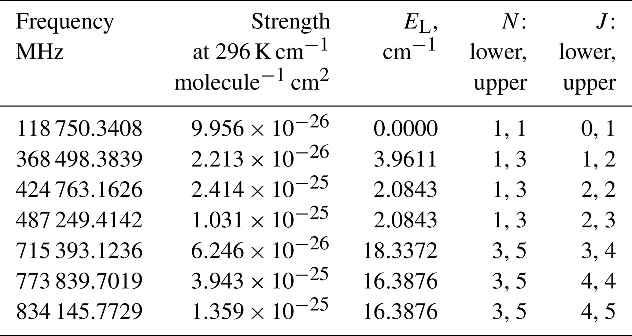
The spectroscopic parameters are taken from the HITRAN database (Rothman et al., 2009). The line strength at the temperature T is as follows:
where J K−1 is the Boltzmann constant, (cm−1) is the transition wavenumber, SH(T0) is the HITRAN line strength (cm−1 cm2 molecule−1), T0=296 K and EL (cm−1) is the lowest energy of the transition. The partition function Q is calculated from tabulated values between 120 and 500 K, a range that encompasses the temperatures found between 50 and 130 km (Q(296)=215.77). The constants CE=102 hp c and allow the conversion of the HITRAN units to the International System (SI) ones. The isotopic ratio riso is taken away from SH and added to the density profile instead. The Table A1 shows parameters of the main O2 millimeter lines.
Above the altitude of about 70 km, the real part of the Voigt function F (Eq. 3) is close to the Gauss function that describes lines broadened by random molecular velocities (Doppler broadening):
with
and Δνd is the Doppler broadening parameter (i.e., the half-width at half-maximum, HWHM) of F, ν0 is the frequency of the transition, m s−1 is the speed of light in vacuum, R=8.31446 J K−1 mol−1 is the gas constant and M is the molar mass (0.031980 kg mol−1 for O2). At 80 km, Δνd is about 0.6–0.7 MHz for the O2 line at 773 GHz, while the pressure broadening HWHM is only 0.01–0.02 MHz.
The dispersion profile used for the calculation of the coefficient q′, u′ and v′ (Eq. 2) is given by the following:
with and t the imaginary error function (Eq. 5.54 in Landi Degl'Innocenti and Landolfi, 2004).
The computation of the matrix exponential in Eq. (1) is the performance bottleneck in our implementation of the radiative transfer solver if we use a general algorithm. A significantly faster algorithm has been implemented using the symmetry in Ko (Eq. 2). The evolution operator Λ (Eq. 8) is written as with ka the scalar absorption coefficient (Eq. 3) and . The Cayley–Hamilton theorem is used to compute :
where is the identity matrix. The coefficient κk are derived using the four eigenvalues of :
where λ1,2 is positive real-valued numbers that determine the four eigenvalues ±λ1 and ±jλ2 of . This gives the following:
The eigenvalue parameters are and , where
and
Model is available upon request.
PB designed the study, performed the simulations and wrote the paper. All co-authors provided valuable information. MS is the PI of the mission proposal.
The authors declare that they have no conflict of interest.
Philippe Baron would like to thank Franz Schreier (German Aerospace Center, DLR) for providing the python implementation of the complex Voigt function used in GARLIC (see reference given for Eq. 3). We would like to thank Hugh C. Pumphrey and the two anonymous referees for their valuable comments that helped us to improve the paper.
SMILES-2 studies are supported by the strategic development research fund from the Institute of Space and Astronautical Science (ISAS)/JAXA. Huixin Liu acknowledges support by JSPS KAKENHI (grants no. 18H01270, 18H04446 and 17KK0095).
This paper was edited by Christian von Savigny and reviewed by Hugh C. Pumphrey and two anonymous referees.
Baron, P., Murtagh, D. P., Urban, J., Sagawa, H., Ochiai, S., Kasai, Y., Kikuchi, K., Khosrawi, F., Körnich, H., Mizobuchi, S., Sagi, K., and Yasui, M.: Observation of horizontal winds in the middle-atmosphere between 30∘ S and 55∘ N during the northern winter 2009–2010, Atmos. Chem. Phys., 13, 6049–6064, https://doi.org/10.5194/acp-13-6049-2013, 2013. a
Baron, P., Manago, N., Ozeki, H., Irimajiri, Y., Murtagh, D., Uzawa, Y., Ochiai, S., Shiotani, M., and Suzuki, M.: Measurement of stratospheric and mesospheric winds with a submillimeter wave limb sounder: Results from JEM/SMILES and simulation study for SMILES-2, in: Sensors, Systems, and Next-Generation Satellites XIX, edited by: Meynart, R., Neeck, S. P., and Shimoda, H., International Society for Optics and Photonics, SPIE, 9639, 140–159, https://doi.org/10.1117/12.2194741, 2015. a
Baron, P., Murtagh, D., Eriksson, P., Mendrok, J., Ochiai, S., Pérot, K., Sagawa, H., and Suzuki, M.: Simulation study for the Stratospheric Inferred Winds (SIW) sub-millimeter limb sounder, Atmos. Meas. Tech., 11, 4545–4566, https://doi.org/10.5194/amt-11-4545-2018, 2018. a, b, c, d, e, f, g
Baron, P., Manago, N., Ochiai, S., and Suzuki, M.: SMILES-2 band selection study for chemical species, IGARSS 2019–2019, Int. Geosci. Remote Se., 7698–7701, https://doi.org/10.1109/IGARSS.2019.8897703, 2019a. a, b
Baron, P., Ochiai, S., Murtagh, D., Sagawa, H., Saito, A., Shiotani, M., and Suzuki, M.: Performance assessment of Super conducting Submillimeter-Wave Limb-Emission Sounder-2 (SMILES-2), IGARSS 2019–2019, Int. Geosci. Remote Se., 7556–7559, https://doi.org/10.1109/IGARSS.2019.8898496, 2019b. a, b, c, d
Baumgarten, G.: Doppler Rayleigh/Mie/Raman lidar for wind and temperature measurements in the middle atmosphere up to 80 km, Atmos. Meas. Tech., 3, 1509–1518, https://doi.org/10.5194/amt-3-1509-2010, 2010. a
Beig, G.: Long-term trends in the temperature of the mesosphere/lower thermosphere region: 1. Anthropogenic influences, J. Geophys. Res.-Space, 116, A00H11, https://doi.org/10.1029/2011JA016646, 2011. a
Chapman, S. and Lindzen, R. S.: Atmospheric tides, D. Reidel Publishing Company and Dordrecht-Holland, Springer Netherlands, 200 pp., https://doi.org/10.1007/978-94-010-3399-2, 1970. a
Christensen, O. M., Eriksson, P., Urban, J., Murtagh, D., Hultgren, K., and Gumbel, J.: Tomographic retrieval of water vapour and temperature around polar mesospheric clouds using Odin-SMR, Atmos. Meas. Tech., 8, 1981–1999, https://doi.org/10.5194/amt-8-1981-2015, 2015. a
Doumbia, V., Maute, A., and Richmond, A. D.: Simulation of equatorial electrojet magnetic effects with the thermosphere-ionosphere-electrodynamics general circulation model, J. Geophys. Res.-Space, 112, A09309, https://doi.org/10.1029/2007JA012308, 2007. a, b
Eastes, R. W., McClintock, W. E., Burns, A. G., Anderson, D. N., Andersson, L., Codrescu, M., Correira, J. T., Daniell, R. E., England, S. L., Evans, J. S., Harvey, J., Krywonos, A., Lumpe, J. D., Richmond, A. D., Rusch, D. W., Siegmund, O., Solomon, S. C., Strickland, D. J., Woods, T. N., Aksnes, A., Budzien, S. A., Dymond, K. F., Eparvier, F. G., Martinis, C. R., and Oberheide, J.: The Global-Scale Observations of the Limb and Disk (GOLD) Mission, Space Sci. Rev., 212, 383–408, https://doi.org/10.1007/s11214-017-0392-2, 2017. a
Englert, C. R., Brown, C. M., Bach, B., Bach, E., Bach, K., Harlander, J. M., Seely, J. F., Marr, K. D., and Miller, I.: High-efficiency echelle gratings for MIGHTI, the spatial heterodyne interferometers for the ICON mission, Appl. Opt., 56, 2090–2098, https://doi.org/10.1364/AO.56.002090, 2017. a, b, c
Forbes, J. M., Russell, J., Miyahara, S., Zhang, X., Palo, S., Mlynczak, M., Mertens, C. J., and Hagan, M. E.: Troposphere-thermosphere tidal coupling as measured by the SABER instrument on TIMED during July–September 2002, J. Geophys. Res.-Space, 111, A10S06, https://doi.org/10.1029/2005JA011492, 2006. a
Fritts, D. C. and Alexander, M. J.: Gravity wave dynamics and effects in the middle atmosphere, Rev. Geophys., 41, 1003, https://doi.org/10.1029/2001RG000106, 2003. a
García-Comas, M., Funke, B., Gardini, A., López-Puertas, M., Jurado-Navarro, A., von Clarmann, T., Stiller, G., Kiefer, M., Boone, C. D., Leblanc, T., Marshall, B. T., Schwartz, M. J., and Sheese, P. E.: MIPAS temperature from the stratosphere to the lower thermosphere: Comparison of vM21 with ACE-FTS, MLS, OSIRIS, SABER, SOFIE and lidar measurements, Atmos. Meas. Tech., 7, 3633–3651, https://doi.org/10.5194/amt-7-3633-2014, 2014. a
Gerber, D., Swinyard, B. M., Ellison, B. N., Plane, J. M. C., Feng, W., Navarathinam, N., Eves, S. J., Bird, R., Linfield, E. H., Davies, A. G., and Parkes, S.: LOCUS: Low cost upper atmosphere sounder, Proc. SPIE, 8889, 88891I, https://doi.org/10.1117/12.2028675, 2013. a
Gumbel, J., Megner, L., Christensen, O. M., Chang, S., Dillner, J., Ekebrand, T., Giono, G., Hammar, A., Hedin, J., Ivchenko, N., Karlsson, B., Kruse, M., Li, A., McCallion, S., Murtagh, D. P., Olentšenko, G., Pak, S., Park, W., Rouse, J., Stegman, J., and Witt, G.: The MATS Satellite Mission – Gravity Waves Studies by Mesospheric Airglow/Aerosol Tomography and Spectroscopy, Atmos. Chem. Phys. Discuss., https://doi.org/10.5194/acp-2018-1162, in review, 2018. a
Hagen, J., Murk, A., Rüfenacht, R., Khaykin, S., Hauchecorne, A., and Kämpfer, N.: WIRA-C: a compact 142-GHz-radiometer for continuous middle-atmospheric wind measurements, Atmos. Meas. Tech., 11, 5007–5024, https://doi.org/10.5194/amt-11-5007-2018, 2018. a
Immel, T. J., Sagawa, E., England, S. L., Henderson, S. B., Hagan, M. E., Mende, S. B., Frey, H. U., Swenson, C. M., and Paxton, L. J.: Control of equatorial ionospheric morphology by atmospheric tides, Geophys. Res. Lett., 33, L15108, https://doi.org/10.1029/2006GL026161, 2006. a
Jacobi, C., Lilienthal, F., Geissler, C., and Krug, A.: Long-term variability of mid-latitude mesosphere-lower thermosphere winds over Collm (51∘ N, 13∘ E), J. Atmos. Sol.-Terr. Phy., 136, 174–186, https://doi.org/10.1016/j.jastp.2015.05.006, 2015. a
Karlsson, B. and Becker, E.: How Does Interhemispheric Coupling Contribute to Cool Down the Summer Polar Mesosphere?, J. Climate, 29, 8807–8821, https://doi.org/10.1175/JCLI-D-16-0231.1, 2016. a
Kaufmann, M., Olschewski, F., Mantel, K., Solheim, B., Shepherd, G., Deiml, M., Liu, J., Song, R., Chen, Q., Wroblowski, O., Wei, D., Zhu, Y., Wagner, F., Loosen, F., Froehlich, D., Neubert, T., Rongen, H., Knieling, P., Toumpas, P., Shan, J., Tang, G., Koppmann, R., and Riese, M.: A highly miniaturized satellite payload based on a spatial heterodyne spectrometer for atmospheric temperature measurements in the mesosphere and lower thermosphere, Atmos. Meas. Tech., 11, 3861–3870, https://doi.org/10.5194/amt-11-3861-2018, 2018. a
Khosravi, M., Baron, P., Urban, J., Froidevaux, L., Jonsson, A. I., Kasai, Y., Kuribayashi, K., Mitsuda, C., Murtagh, D. P., Sagawa, H., Santee, M. L., Sato, T. O., Shiotani, M., Suzuki, M., von Clarmann, T., Walker, K. A., and Wang, S.: Diurnal variation of stratospheric and lower mesospheric HOCl, ClO and HO2 at the equator: comparison of 1-D model calculations with measurements by satellite instruments, Atmos. Chem. Phys., 13, 7587–7606, https://doi.org/10.5194/acp-13-7587-2013, 2013. a
Kikuchi, K., Nishibori, T., Ochiai, S., Ozeki, H., Irimajiri, Y., Kasai, Y., Koike, M., Manabe, T., Mizukoshi, K., Murayama, Y., Nagahama, T., Sano, T., Sato, R., Seta, M., Takahashi, C., Takayanagi, M., Masuko, H., Inatani, J., Suzuki, M., and Shiotani, M.: Overview and early results of the Superconducting Submillimeter-Wave Limb-Emission Sounder (SMILES), J. Geophys. Res., 115, D23306, https://doi.org/10.1029/2010JD014379, 2010. a
Landi Degl'Innocenti, M. and Landolfi, M.: Polarization in Spectral Lines, Astrophysics and Space Science Library, Springer Netherlands, https://books.google.co.jp/books?id=8sl2CkmZNWIC, 2004. a, b, c, d, e
Larsson, R., Ramstad, R., Mendrok, J., Buehler, S. A., and Kasai, Y.: A method for remote sensing of weak planetary magnetic fields: Simulated application to Mars, Geophys. Res. Lett., 40, 5014–5018, https://doi.org/10.1002/grl.50964, 2013. a
Larsson, R., Buehler, S. A., Eriksson, P., and Mendrok, J.: A treatment of the Zeeman effect using Stokes formalism and its implementation in the Atmospheric Radiative Transfer Simulator (ARTS), J. Quant. Spectrosc. Ra., 133, 445–453, https://doi.org/10.1016/j.jqsrt.2013.09.006, 2014. a, b, c, d, e
Larsson, R., Lankhaar, B., and Eriksson, P.: Updated Zeeman effect splitting coefficients for molecular oxygen in planetary applications, J. Quant. Spectrosc. Ra., 224, 431–438, https://doi.org/10.1016/j.jqsrt.2018.12.004, 2019. a
Lenoir, W. B.: Microwave spectrum of molecular oxygen in the mesosphere, J. Geophys. Res., 73, 361–376, https://doi.org/10.1029/JA073i001p00361, 1968. a, b
Mlynczak, M. G. and Yee, J. H.: LATTICE: The Lower Atmosphere-Thermosphere-Ionosphere Coupling Experiment, AGU Fall Meeting Abstracts, 1, 2017. a
Navas-Guzmán, F., Kämpfer, N., Murk, A., Larsson, R., Buehler, S. A., and Eriksson, P.: Zeeman effect in atmospheric O2 measured by ground-based microwave radiometry, Atmos. Meas. Tech., 8, 1863–1874, https://doi.org/10.5194/amt-8-1863-2015, 2015. a
Niciejewski, R., Wu, Q., Skinner, W., Gell, D., Cooper, M., Marshall, A., Killeen, T., Solomon, S., and Ortland, D.: TIMED Doppler Interferometer on the Thermosphere Ionosphere Mesosphere Energetics and Dynamics Satellite: Data product overview, J. Geophys. Res.-Space, 111, A11S90, https://doi.org/10.1029/2005JA011513, 2006. a
Ochiai, S., Kikuchi, K., Nishibori, T., Manabe, T., Ozeki, H., Mizobuchi, S., and Irimajiri, Y.: Receiver Performance of the Superconducting Submillimeter-Wave Limb-Emission Sounder (SMILES) on the International Space Station, IEEE T. Geosci. Remote, 51, 3791–3802, https://doi.org/10.1109/TGRS.2012.2227758, 2013. a
Ochiai, S., Baron, P., Nishibori, T., Irimajiri, Y., Uzawa, Y., Manabe, T., Maezawa, H., Mizuno, A., Nagahama, T., Sagawa, H., Suzuki, M., and Shiotani, M.: SMILES-2 mission for temperature, wind, and composition in the whole atmosphere, SOLA, 13A, 13–18, https://doi.org/10.2151/sola.13A-003, 2017. a, b, c, d
Ochiai, S., Baron, P., Irimajiri, Y., Uzawa, Y., Nishibori, T., Akinori, S., Suzuki, M., and Shiotani, M.: Superconducting Submillimeter-Wave Limb-Emission Sounder, SMILES-2, for middle and upper atmospheric study, IGARSS 2018–2018, IEEE T. Geosci. Remote, 9153–9156, https://doi.org/10.1109/IGARSS.2018.8518300, 2018. a
Ochiai, S., Baron, P., Irimajiri, Y., Nishibori, T., Hasegawa, T., Uzawa, Y., Maezawa, H., Manabe, T., Mizuno, A., Nagahama, T., Kimura, K., Suzuki, M., Saito, A., and Shiotani, M.: Conceptual study of Superconducting Submillimeter-Wave Limb-Emission Sounder-2 (SMILES-2) receiver, IGARSS 2019–2019, IEEE T. Geosci. Remote, 8792–8795, https://doi.org/10.1109/IGARSS.2019.8898693, 2019. a
Pancheva, D. and Mukhtarov, P.: Atmospheric Tides and Planetary Waves: Recent Progress Based on SABER/TIMED Temperature Measurements (2002–2007), Springer Netherlands, Dordrecht, 19–56, https://doi.org/10.1007/978-94-007-0326-1_2, 2011. a
Pardo, J., Pagani, L., Gerin, M., and Prigent, C.: Evidence of the zeeman splitting in the rotational transition of the atmospheric 16O18O molecule from ground-based measurements, J. Quant. Spectrosc. Ra., 54, 931–943, https://doi.org/10.1016/0022-4073(95)00129-9, 1995. a
Rodgers, C. D.: Inverse Methods for Atmospheric Sounding: Theory and Practise, 2 of Series on Atmospheric, Oceanic and Planetary Physics, World Scientific, 256 pp., https://doi.org/10.1142/3171, 2000. a
Rothman, L., Gordon, I., Barbe, A., Benner, D., Bernath, P., Birk, M., Boudon, V., Brown, L., Campargue, A., Champion, J.-P., Chance, K., Coudert, L., Dana, V., Devi, V., Fally, S., Flaud, J.-M., Gamache, R., Goldman, A., Jacquemart, D., Kleiner, I., Lacome, N., Lafferty, W., Mandin, J.-Y., Massie, S., Mikhailenko, S., Miller, C., Moazzen-Ahmadi, N., Naumenko, O., Nikitin, A., Orphal, J., Perevalov, V., Perrin, A., Predoi-Cross, A., Rinsland, C., Rotger, M., Smith, M., Sung, K., Tashkun, S., Tennyson, J., Toth, R., Vandaele, A., and Auwera, J. V.: The HITRAN 2008 molecular spectroscopic database, J. Quant. Spectrosc. Ra., 110, 533–572, https://doi.org/10.1016/j.jqsrt.2009.02.013, 2009. a
Rüfenacht, R., Murk, A., Kämpfer, N., Eriksson, P., and Buehler, S. A.: Middle-atmospheric zonal and meridional wind profiles from polar, tropical and midlatitudes with the ground-based microwave Doppler wind radiometer WIRA, Atmos. Meas. Tech., 7, 4491–4505, https://doi.org/10.5194/amt-7-4491-2014, 2014. a
Sakazaki, T., Fujiwara, M., Mitsuda, C., Imai, K., Manago, N., Naito, Y., Nakamura, T., Akiyoshi, H., Kinnison, D., Sano, T., Suzuki, M., and Shiotani, M.: Diurnal ozone variations in the stratosphere revealed in observations from the Superconducting Submillimeter-Wave Limb-Emission Sounder (SMILES) on board the International Space Station (ISS), J. Geophys. Res.-Atmos., 118, 2991–3006, https://doi.org/10.1002/jgrd.50220, 2013. a
Sakazaki, T., Sato, K., Kawatani, Y., and Watanabe, S.: Three-dimensional structures of tropical nonmigrating tides in a high-vertical-resolution general circulation model, J. Geophys. Res.-Atmos., 120, 1759–1775, https://doi.org/10.1002/2014JD022464, 2015. a
Sato, K., Yasui, R., and Miyoshi, Y.: The Momentum Budget in the Stratosphere, Mesosphere, and Lower Thermosphere, Part I: Contributions of Different Wave Types and In Situ Generation of Rossby Waves, J. Atmos. Sci., 75, 3613–3633, https://doi.org/10.1175/JAS-D-17-0336.1, 2018. a
Schreier, F., Garcia, S. G., Hedelt, P., Hess, M., Mendrok, J., Vasquez, M., and Xu, J.: GARLIC – A general purpose atmospheric radiative transfer line-by-line infrared-microwave code: Implementation and evaluation, J. Quant. Spectrosc. Ra., 137, 29–50, https://doi.org/10.1016/j.jqsrt.2013.11.018, 2014. a, b
Schwartz, M. J., Read, W. G., and Snyder, W. V.: EOS MLS forward model polarized radiative transfer for Zeeman-split oxygen lines, IEEE T. Geosci. Remote, 44, 1182–1191, https://doi.org/10.1109/TGRS.2005.862267, 2006. a, b, c, d, e
Semel, M. and López, A.: Integration of the radiative transfer equation for polarized light: The exponential solution, A&A, 342, 201–211, 1999. a
Sheese, P. E., Llewellyn, E. J., Gattinger, R. L., Bourassa, A. E., Degenstein, D. A., Lloyd, N. D., and McDade, I. C.: Temperatures in the upper mesosphere and lower thermosphere from OSIRIS observations of O2 A-band emission spectra, Can. J. Phys., 88, 919–925, https://doi.org/10.1139/p10-093, 2010. a
Shepherd, G. G.: Development of wind measurement systems for future space missions, Acta Astronaut., 115, 206–217, https://doi.org/10.1016/j.actaastro.2015.05.015, 2015. a
Shiotani, M., Saito, A., Sakazaki, T., Ochiai, S., Baron, P., Nishibori, T., Suzuki, M., Abe, T., Maezawa, H., and Oyama, S.: A proposal for satellite observation of the whole atmosphere – Superconducting Submillimeter-Wave Limb-Emission Sounder-2 (SMILES-2), IGARSS 2019–2019, IEEE T. Geosci. Remote, 8788–8791, https://doi.org/10.1109/IGARSS.2019.8898423, 2019. a, b
Sica, R. J., Izawa, M. R. M., Walker, K. A., Boone, C., Petelina, S. V., Argall, P. S., Bernath, P., Burns, G. B., Catoire, V., Collins, R. L., Daffer, W. H., De Clercq, C., Fan, Z. Y., Firanski, B. J., French, W. J. R., Gerard, P., Gerding, M., Granville, J., Innis, J. L., Keckhut, P., Kerzenmacher, T., Klekociuk, A. R., Kyrö, E., Lambert, J. C., Llewellyn, E. J., Manney, G. L., McDermid, I. S., Mizutani, K., Murayama, Y., Piccolo, C., Raspollini, P., Ridolfi, M., Robert, C., Steinbrecht, W., Strawbridge, K. B., Strong, K., Stübi, R., and Thurairajah, B.: Validation of the Atmospheric Chemistry Experiment (ACE) version 2.2 temperature using ground-based and space-borne measurements, Atmos. Chem. Phys., 8, 35–62, https://doi.org/10.5194/acp-8-35-2008, 2008. a
Smith, A. K.: Global Dynamics of the MLT, Surv. Geophys., 33, 1177–1230, https://doi.org/10.1007/s10712-012-9196-9, 2012. a, b
Steinbrecht, W., McGee, T. J., Twigg, L. W., Claude, H., Schönenborn, F., Sumnicht, G. K., and Silbert, D.: Intercomparison of stratospheric ozone and temperature profiles during the October 2005 Hohenpeißenberg Ozone Profiling Experiment (HOPE), Atmos. Meas. Tech., 2, 125–145, https://doi.org/10.5194/amt-2-125-2009, 2009. a
Steiner, O., Züger, F., and Belluzzi, L.: Polarized radiative transfer in discontinuous media, A42, 586, 14 pp., https://doi.org/10.1051/0004-6361/201527158, 2016. a
Tsuda, T.: Characteristics of atmospheric gravity waves observed using the MU (Middle and Upper atmosphere) radar and GPS (Global Positioning System) radio occultation, P. Jpn. Acad., 90, 12–27, 2014. a
Tsutsumi, M., Sato, K., Sato, T., Kohma, M., Nakamura, T., Nishimura, K., and Tomikawa, Y.: Characteristics of Mesosphere Echoes over Antarctica Obtained Using PANSY and MF Radars, SOLA, 13A, 19–23, https://doi.org/10.2151/sola.13A-004, 2017. a
Urban, J., Baron, P., Lautié, N., Schneider, N., Dassas, K., Ricaud, P., and De La Noë, J.: MOLIERE (v5): a versatile forward- and inversion model for the millimeter and sub-millimeter wavelength range, J. Quant. Spectrosc. Ra. 83, 529–554, https://doi.org/10.1016/S0022-4073(03)001040-3, 2004. a
Wang, W., Wang, Z., and Duan, Y.: Performance evaluation of THz Atmospheric Limb Sounder (TALIS) of China, Atmos. Meas. Tech., 13, 13–38, https://doi.org/10.5194/amt-13-13-2020, 2020. a
Wu, D. L., Schwartz, M. J., Waters, J. W., Limpasuvan, V., Wu, Q. A., and Killeen, T. L.: Mesospheric doppler wind measurements from Aura Microwave Limb Sounder (MLS), Adv. Space Res., 42, 1246–1252, 2008. a
Wu, D. L., Yee, J.-H., Schlecht, E., Mehdi, I., Siles, J., and Drouin, B. J.: THz limb sounder (TLS) for lower thermospheric wind, oxygen density, and temperature, J. Geophys. Res.-Space, 121, 7301–7315, https://doi.org/10.1002/2015JA022314, 2016. a
Xu, X., Manson, A. H., Meek, C. E., Chshyolkova, T., Drummond, J. R., Hall, C. M., Riggin, D. M., and Hibbins, R. E.: Vertical and interhemispheric links in the stratosphere-mesosphere as revealed by the day-to-day variability of Aura-MLS temperature data, Ann. Geophys., 27, 3387–3409, https://doi.org/10.5194/angeo-27-3387-2009, 2009. a
Yamazaki, Y. and Maute, A.: Sq and EEJ – A Review on the Daily Variation of the Geomagnetic Field Caused by Ionospheric Dynamo Currents, Space Sci. Rev., 206, 299–405, https://doi.org/10.1007/s11214-016-0282-z, 2017. a
Yee, J. H., Gjerloev, J., Wu, D., and Schwartz, M. J.: First Application of the Zeeman Technique to Remotely Measure Auroral Electrojet Intensity From Space, Geophys. Res. Lett., 44, 10134–10139, https://doi.org/10.1002/2017GL074909, 2017. a, b, c, d, e, f
Yi, W., Xue, X., Reid, I. M., Murphy, D. J., Hall, C. M., Tsutsumi, M., Ning, B., Li, G., Vincent, R. A., Chen, J., Wu, J., Chen, T., and Dou, X.: Climatology of the mesopause relative density using a global distribution of meteor radars, Atmos. Chem. Phys., 19, 7567–7581, https://doi.org/10.5194/acp-19-7567-2019, 2019. a
- Abstract
- Introduction
- Measurement principle
- Zeeman effect modeling
- Measurement and retrieval setting
- Retrieval errors
- Conclusions
- Appendix A: Spectroscopic parameters
- Appendix B: Matrix exponential
- Code availability
- Author contributions
- Competing interests
- Acknowledgements
- Financial support
- Review statement
- References