2.1 Fundamentals of tuneable diode laser heterodyne spectroradiometry

The basic principles of the diode laser heterodyne spectroradiometry (TDLHS) have been presented in detail in previous works, e.g., in Rodin et al. (2014), Kurtz and O'Byrne (2016), and Zenevich et al. (2019). Here we briefly repeat the core information important for Doppler measurements. In contrast with conventional microwave heterodyne spectroradiometry, TDLHS operates with a tuneable local oscillator (LO) – a diode laser with distributed feedback (DFB), characterized by a bandwidth of about 2 MHz and capable of changing its radiation frequency in a broad spectral range. Typically, two parameters are employed to control DFB laser radiation frequency, namely its temperature and injection current. Temperature affects the resonant frequency through the period of an embedded Bragg grating, while pumping current impacts both grating period (through temperature variations according to absorbed power) and refractive index (through charge carrier density). Commercial DFB lasers are supplied with embedded Peltier coolers and thermal sensors, so both parameters could be precisely controlled by external electronics.

We apply the algorithm of LO sweeping with locking to reference the absorption line, as described in Rodin et al. (2014). According to this algorithm, the temperature controller is set at a constant value, while the pumping current is modulated by a piecewise linear saw-edged function. Both laser power and wavelength change accordingly. The signal acquired simultaneously in the heterodyne channel is characterized by linear growth of the received power according to changing LO intensity and by a random heterodyne component:

where D is the detector responsivity, g_LO and F_S are power spectral densities of the LO and solar light at LO frequency, while φ_LO and φ_S are their respective phases. The power spectrum of the beat signal is proportional to the convolution of power spectra related to the signal F_S and local oscillator S_LO, respectively:

As the analyzed solar radiation is not expected to reveal features narrower than the LO bandwidth, i.e., F_S may be assumed constant within the bandwidth B corresponding to the peak of S_LO. This may in turn be replaced by the delta function, and the convolution on the right-hand side of Eq. (2) could be reduced to a simple product. Due to the random phase factor within a narrow frequency range with respect to LO bandpass, Δω≤Δω_LO, the heterodyne signal reveals properties of a white noise with the dispersion proportional to the target spectral density F_S:

Therefore, to achieve heterodyning of the thermal non-coherent IR radiation, one needs, at first, to subtract a linear component from the signal associated with sweeping the LO power and then to obtain the dispersion by square detection. Finally, appropriate exposure and data collection provide target spectrum F_S(ω) with the required signal-to-noise ratio. Taking into account that the LO linewidth has an order of 2 MHz, the spectral resolution of heterodyne detection is sufficient to measure the Doppler shift of the absorption line in the atmosphere due to air mass motion with along line-of-sight velocities greater than 3 m s⁻¹ by providing high LO stability and sufficient accuracy of intermediate frequency (IF) signal analysis. Note that sweeping the LO frequency over a spectral range of interest and replacement IF spectral analysis by mere dispersion evaluation implies a much simpler instrument design compared to conventional heterodyne spectroradiometers, as complex back-end equipment is no longer necessary. Further details of data treatment depend on the optical scheme and should be discussed in the link with description of the experimental setup.

2.2 Experimental setup and observations

A detailed description of the experimental setup is presented in Zenevich et al. (2019). Here we briefly repeat the main information important for understanding. A sketch of the experimental laser heterodyne spectroradiometer (LHS) is presented in Fig. 1. Solar radiation passing through the atmosphere is focused to the edge of a single-mode silica optical fiber with core diameter ∼10 µm by a lens with focal length f=50 mm. A chopper installed in front of the fiber allows one to record the heterodyne signal with the Sun's radiation on and off. Thus the dark signal, dominated by the shot noise, and superposition of the heterodyne and dark signals are measured separately. This technique provides accurate subtraction of the shot noise unaffected by possible system drifts of the instrument. Sunlight entering the fiber has been combined with an LO radiation in a single-mode silica coupler with a 5:95 coupling ratio. According to the antenna theorem (Siegman, 1966), the single-mode fiber geometric aperture factor is $\sim \mathrm{2.6}\times {\mathrm{10}}^{-\mathrm{8}}$ cm², which corresponds to field of view ∼0.006^∘. This is close to the maximum available for heterodyne detection and therefore does not limit the instrument sensitivity (Rodin et al., 2014). An automated Sky-Watcher EQ6 PRO SynScan equatorial mount equipped with a QHY5-II guide camera was used to track the Sun during observations.

Figure 1The sketch of a laser heterodyne spectrometer used for wind profiling.

Download

The radiation of the NEL DFB laser serving as an LO is split into 50:50 proportion, with one portion being coupled with solar radiation in the heterodyne channel and another portion being put into the reference cell. All fiber optical connections in both the heterodyne and the reference channels are made by welding, with the exception of two FC/APC angled connectors to the LO and to the telescope, to avoid undesired reflection, which may otherwise significantly contaminate the signal with parasite interference pattern. Frequency ramping in the range 6230.2±0.35 cm⁻¹ was provided due to modulation of the pumping current by a chain of pulses, with a pulse length of 39.4 ms, a dead time of 10.6 ms, and a stepwise current growth within a pulse with a step length of 200 µs. The cell filled with CO₂ at a pressure of 13 Torr is an off-axis resonator with the input and output mirrors reflectivity R_in=0.9998 and R_out=0.98, respectively, which provides the effective optical path length ∼30 m. This path allows for a reliable measurement of the Doppler-broadened contour of the weak absorption line in the 1.605 µm band by means of the integrated cavity output spectroscopy (ICOS) technique (Moyer et al., 2008). Negative feedback between the detected line position in the reference cell and diode laser crystal temperature has been organized in order to stabilize the LO frequency ramping and to avoid drifts, with the crystal temperature correction accuracy of 10⁻⁴ K. Although line shape in the ICOS cell is different from the Voigt profile, it does not affect the LO stabilization procedure, as the only information used in the feedback concerns the peak position. After coupling solar radiation with the LO, a single-mode fiber transmits the signal into a Hamamatsu InGaAs PIN photodiode serving as a heterodyne mixer. Then the beat signal is analyzed with back-end electronics.

After the transimpedance preamplifier, the signal is passed through a consecutive low-pass filter, another amplifier, and high-pass filter that limits its bandwidth to 0.2 to 3 MHz. The preamplifier circuit is connected to a Rohde & Schwarz RTO 1012 digital oscilloscope at two points as follows: after the IF receiver and just after the transimpedance preamplifier. The latter signal repeats the LO pumping current pulse shape and is utilized for oscilloscope synchronization with the LO ramping cycle. The first is used for dispersion evaluation and data collection. The oscilloscope translates the signal into a digital sequence with the rate of 20 000 points per second, then calculates the dispersion, and averages data in a similar way as it has been previously done by Wilson et al. (2014) and Kurtz and O'Byrne (2016). The oscilloscope communicates with the PC by Ethernet channel, while the other parts of the setup, including the LO control system and Sun tracker, are connected by USB. Instrument control and data transfer are implemented based on the LabVIEW platform.

As the correct frequency calibration over the whole range of LO ramping is crucial for Doppler analysis of the atmospheric absorption, we employed another reference channel based on a Fabry–Pérot etalon. Frequency calibrations were done offline, as described in Rodin et al. (2014), and utilized for processing and interpretation of atmospheric absorption measurements. In order to estimate the accuracy of frequency absolute stabilization by the reference cell and relative calibration by a Fabry–Pérot etalon, deviations in LO frequency ramping from the prescribed sequence were tracked along several hours. These tests have shown a root mean square deviation of 1.5 MHz in the vicinity of the reference CO₂ line and 6 MHz in the rest of the LO ramping range.

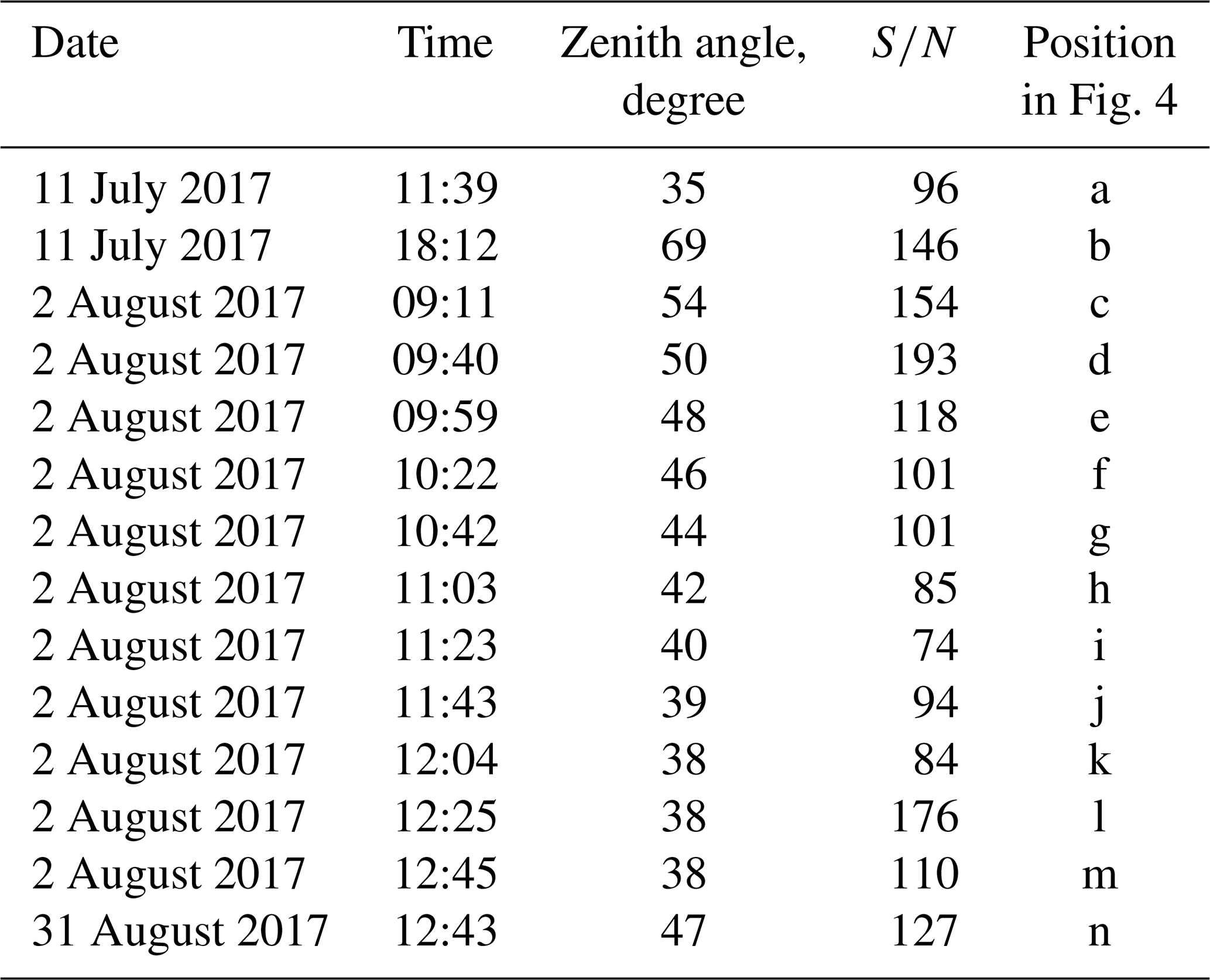
Several observation sessions were carried out during the summer of 2018 under clear sky conditions. The instrument was installed at the top of one of the buildings at the MIPT campus in the north of Moscow, with coordinates 55.929036^∘ N, 37.521506^∘ E, about 50 m above sea level. Data were collected for ∼10 min, to reach a signal-to-noise level of 100. The details of observations and some key characteristics of the retrieved spectra are presented in Table 1.

Table 1Observations of CO₂ absorption line profile.

Download Print Version | Download XLSX

3.1 Raw data treatment

Once the heterodyne signal is obtained, one needs to subtract the corresponding dark signal with the solar channel being closed by a chopper. The next step is to eliminate the baseline slope caused by the modulation of the LO power. Since the heterodyne signal and shot noise have the same statistical nature which is proportional to the power absorbed by a photomixer, this slope cannot be eliminated by dark signal subtraction and requires model approximation of the spectral continuum outside the observed absorption line. After subtraction of the dark signal, the heterodyne signal should be normalized by assumed spectral continuum (baseline) approximated by square polynomial to obtain the final transmission spectrum of the atmosphere. Consecutive steps of raw data treatment are presented in Fig. 2a–c. In Fig. 2a one could notice a baseline distortion in the reference channel caused by the residual interference in the ICOS multipass cell. This distortion may be eliminated by a precise adjustment of the entrance beam. However, this channel is only used for the determination of the line peak position, which is not sensitive to the baseline variations.

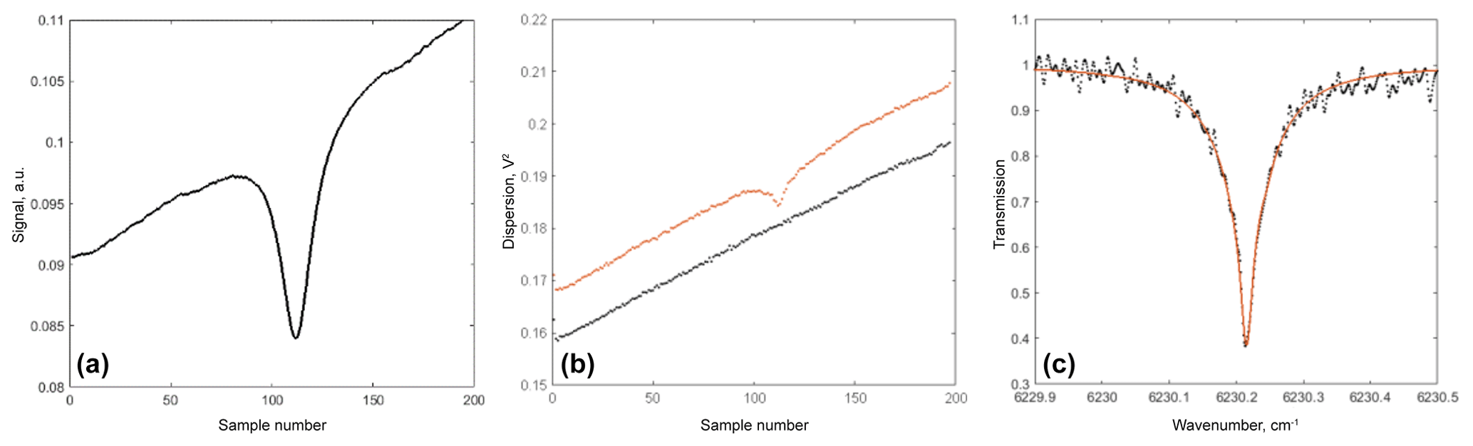
Figure 2Heterodyne signal treatment in the LHS: (a) signal in the reference channel during one cycle of laser pumping current ramping; (b) noise dispersion in the heterodyne channel during one cycle of laser pumping current ramping; blue dots – with the Sun off, red dots – with the Sun on; (c) atmospheric transmission spectrum obtained after removing dark signal, normalization to suggested continuum (baseline), and frequency calibration. Black dots – experiment, red curve – model fit.

Download

Further treatment of the LHS data implies a comparison with a synthetic spectrum of the atmospheric transmission. Since in the narrow field of view of the LHS the scattered component is negligible compared to direct solar radiation, the simulation of atmospheric spectra is straightforward. In addition to the target CO₂ line R2 14⁰1←00⁰0 at 6230.22 cm⁻¹, other CO₂ lines at 6230.25, 6230.02, and 6229.98 cm⁻¹ have also been included in the calculations. Other atmospheric species, including water vapor, do not affect this spectral range with features that could be distinguished from the spectral continuum. Based on HITRAN2016 data (Gordon et al., 2017), a model of the atmospheric transmission spectrum has been constructed. In the calculations we used the Voight line shape and neglected line mixing and other fine effects that may affect line shape in its far wings (Armstrong, 1982; Bulanin et al., 1984; Boone et al., 2011). Although such a simplistic approach may appear insufficient for the analysis of a fully resolved line profile, the experiments presented below show that the model fits observations within data errors. Peculiar exceptions, including poor fitting to the Doppler-broadened line core described below, do not affect wind retrievals as the contribution of this narrow spectral range to the retrieval procedure is negligible.

The modeled atmosphere includes 100 uniform layers with constant gas composition, pressure, temperature, and wind. The upper boundary of the modeled atmosphere is determined by the condition that maximal absorption in the uppermost layer did not exceed 0.1 % of the total absorption. The model only included gas absorption in the lines mentioned above, whereas scattering processes have been neglected. Minor effects of the second order in terms of line-of-sight curve, such as atmospheric refraction and sphericity of the atmosphere, have been neglected as well. The model does not pretend to provide a precise calculation of the net absorption, as would be required for CO₂ column amounts retrievals, because it is line shape rather than line depth that contains information about the line-of-sight wind component. An example of line shape fit by radiative transfer model involving Doppler line distortion is presented in Fig. 2c by the red curve. It is evident that the line shape in the atmospheric column shown in Fig. 2c is different from that detected in the reference cell (Fig. 2a). The atmospheric line reveals a sharper tip and broader wings due to the superposition of absorption characterized by different broadening at different altitudes. Broader wings dominated by a collisional Lorentzian broadening profile are formed in the troposphere, whereas a narrow, Doppler-broadened tip is formed in the stratosphere and mesosphere. It is this line shape, which provides information about vertical variations of atmospheric conditions, that provides a clue to wind profile retrievals from LHS data.

Wind affects the model spectrum by Doppler shift of the line at each particular model layer, with the transmittance spectrum line shape and absorption value corresponding to the local pressure, temperature, and CO₂ concentration. Indeed, lower atmospheric layers contribute more effectively to the wings of the line profile, whereas a line peak dominated by Doppler thermal broadening is formed at higher altitudes. Therefore, by providing a nonuniform profile of wind projection on the line of sight, the observed line profile is distorted rather than shifted in the frequency scale. This fact gives an opportunity for the line-of-sight component of the wind profile retrieval based on analysis of the resolved line shape.

3.2 Solution to the inverse problem of wind profiling based on the high-resolution NIR absorption spectrum

The inverse problems of radiative transfer are similar to those stated above; i.e., the wind projection profile retrievals from the absorption line shape that are observed through the atmospheric column suffer from mathematical ill-posedness. This means that a solution is not unique and/or reveals instability when compared to small variations of data; thus, in this case a solution is based on Hadamard (1902). Since TDLHS introduces a certain noise level to data by nature, noisy data force the instability of a solution unless special measures for solution regularization are taken. In this work we consider the generalized residual method of regularization (GRM), similar in many aspects to Tikhonov regularization, yet highly efficient in cases when some a priori assumption on solution properties could be made (Tikhonov, 1998).

Let us consider a radiative transfer model, taking into account Doppler distortion of the absorption spectrum:

where $\mathit{\tau }\left(\mathit{\vartheta }\right)=-\ln \left(T\left(\mathit{\vartheta }\right)\cos \left(\mathit{\theta }\right)\right)$ is optical depth normalized for vertical path at wavenumber ϑ, T(ϑ) is observed atmospheric transmission, θ is the Sun zenith angle, ρ(z) is assumed number density of CO₂ molecules, U(z) is assumed vertical profile of wind projection on the line of sight, c is the speed of light, ϑ₀ is a wavenumber of the line center, and the function σ(ϑ,z) is a model absorption cross section at wavenumber ϑ and altitude z per molecule calculated according to the algorithm described above. Equation (4) may be rewritten in the operator form:

or, assuming a nearly uniform vertical distribution of carbon dioxide in the atmospheric column and replacing vector $\stackrel{\mathrm{‾}}{\mathit{\rho }}$ with a scalar parameter ρ,

It was first noticed by Tikhonov (1943) that a solution $\stackrel{\mathrm{‾}}{\mathit{U}}$ to Eq. (6) reveals stability in RHS provided it is searched for on a compact set $M{W}_{\mathrm{2}}^{\mathrm{1}}$. The GRM implies the introduction of a stabilizing functional Ω(U,ρ) which is physically sensible and obeys special properties, e.g., is concave and semicontinuous, to provide method convergence (Amato and Hughes, 1991). Such a functional may be constructed according to the maximum entropy method:

Function g(U) is introduced to provide convexity of the functional Ω_ε(U), g(U) and is a smooth function taken in the form $g\left(U\right)=\sqrt{U^{\mathrm{2}}+\mathit{\epsilon }}$ with a small epsilon ε=0.001, and the approximation property $\left|{\mathrm{\Omega }}_{\mathit{\epsilon }}\left(U\right)-\mathrm{\Omega }\left(U\right)\right|<\mathit{\epsilon }k$ (k is a constant) so that the solution should be searched for on the compact set $M=\left\{\mathrm{\Omega }\left(\stackrel{\mathrm{‾}}{\mathit{U}},\stackrel{\mathrm{‾}}{\mathit{\rho }}\right)\le {\mathrm{\Omega }}_{\mathit{\delta }}\right\}$. As a result, the solution is obtained by constrained minimization of the stabilizing functional provided that model deviation from the data set does not exceed expected measurement error:

The choice of maximal entropy as a solution regularization criterion is closely related to the nature of its uncertainty. Indeed, the vertical wind profile from the ground to mesosphere is determined by a number of factors and is therefore not expected to obey any special properties but smoothness caused by averaging over kernels shown in Fig. 3. However, it is known a priori that the retrievals are based on observed line shapes (see Fig. 2b) and may not contain information exceeding the limited amounts delivered by those data. Any extra information added during the data treatment process may only decrease the quality of the retrievals. Therefore, among solutions compatible with observations, those obeying minimal information would be considered the best. Since information is by definition equivalent to entropy up to a sign, the smoothing functional (Eq. 7) reflecting the maximal entropy principle selects the best solution to the inverse problem (Eq. 6). Once the regularization criterion is selected, the problem (Eq. 8) could be efficiently solved by sequential quadratic programming methods (Spellucci, 1998), resulting in a vertical profile of wind projection on the line of sight of Sun observation.

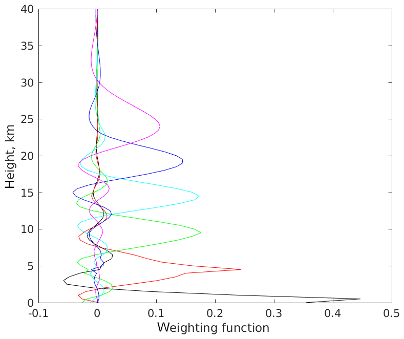
Figure 3Weighting kernels of wind retrievals according to Eq. (10) as functions of altitude. Kernels corresponding to reference heights of 0, 5, 10, 15, 20, and 25 km are presented.

Download

In order to estimate potential uncertainties introduced by the retrievals, it is instructive to linearize the problem (Eq. 6) in the proximity of some assumed solution $\stackrel{\mathrm{‾}}{{\mathit{U}}_{\mathbf{0}}}$:

where ${\widehat{A}}^{\prime }$ is an operator of the initial radiative transfer problem (Eq. 6) linearized in wind velocity projection $\stackrel{\mathrm{‾}}{\mathit{U}}$. It is convenient to use the classical Tikhonov functional which is the non-constrained analog of the GRM method with the Lagrange additional parameter α:

Then the Jacobian of the regularized inverse operator may be written in a matrix form, where I is a Jacobian matrix of the sub-integral function in Eq. (7):

where α is a regularization parameter which can be determined according to the residual principle (Tikhonov, 1998). Here the function ρ(α) is monotonically increasing according to the α parameter $\mathit{\rho }\left(\mathit{\alpha }\right)={∥\mathbf{A}\mathit{U}-\mathit{\tau }∥}^{\mathrm{2}}={\mathit{\delta }}^{\mathrm{2}}$, and in our case we have $\mathit{\alpha }=\mathrm{2.43}\times {\mathrm{10}}^{-\mathrm{5}}$. The linearized solution will take the form $\stackrel{\mathrm{‾}}{\mathit{U}}{}^{\prime }={\mathit{\rho }}^{-\mathrm{1}}\widehat{\mathbf{K}}\left(\stackrel{\mathrm{‾}}{\mathit{\tau }}-\stackrel{\mathrm{‾}}{{\mathit{\tau }}_{\mathbf{0}}}\right)+\stackrel{\mathrm{‾}}{{\mathit{U}}_{\mathbf{0}}}$ or $\stackrel{\mathrm{‾}}{\mathit{U}}={\mathit{\rho }}^{-\mathrm{1}}\widehat{\mathbf{K}}\mathit{d}\stackrel{\mathrm{‾}}{\mathit{\tau }}$. The averaging kernel which characterizes the sensitivity of a regularized solution $\stackrel{\mathrm{‾}}{\mathit{U}}{}^{\prime }$ to exactly one $\stackrel{\mathrm{‾}}{\mathit{U}}$ is defined as follows (see Rodgers, 2000):

Examples of averaging kernels are presented in Fig. 4, depending on altitude. Each curve corresponds to that particular altitude at which the exact solution is defined so that one may consider it as a point spread function associated with the regularization procedure. Therefore, the characteristic width of the main peak of the averaging kernel is a measure of the effective vertical resolution of the method. It is seen from Fig. 4 that the resolution is higher in the lower part of the profile and reaches a few kilometers near the ground, whereas in higher altitudes it is comparable with one scale height. Another important feature of the kernel is the presence of negative secondary peaks which may, for some particular wind profiles, generate unrealistic oscillations in retrievals. Nevertheless, the shape of averaging kernels that demonstrates sharp main peaks and regular structure provides an opportunity for sensible recovery of wind projection profiles from the lower troposphere to mesosphere, with the vertical resolution better than one scale height. Note that average kernels and, hence, vertical resolution of wind retrievals are determined by collisional linewidth and signal-to-noise ratio rather than on the spectral resolution of the instrument, which is excessively high for such retrievals.

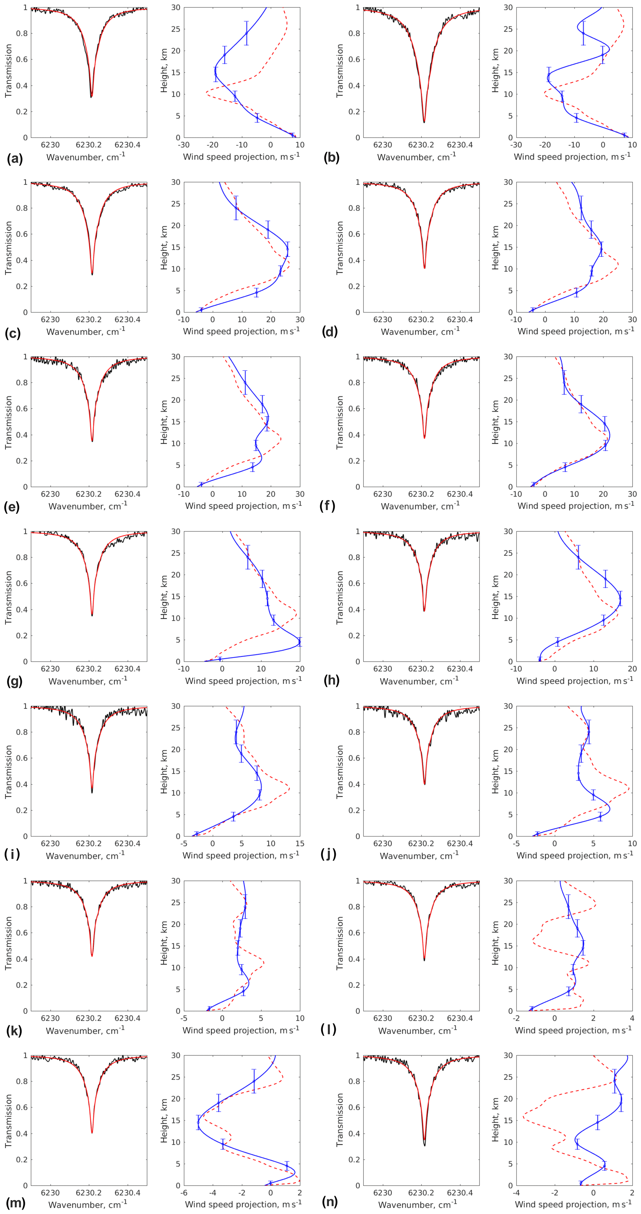
Figure 4Comparison of retrieved wind projection on the line of sight (right panels, blue curve) with reanalysis data (red dashed curve). Vertical error bars correspond to FWHM of a retrieval averaging kernel presented in Fig. 3. Left panels show atmospheric transmission spectrum measured by means of heterodyne technique (black curve) and the corresponding best-fit model spectrum (red curve). Date and local time of each observation are presented in Table 1.

Download

3.3 Results

The analysis of data received during three observation sessions in summer 2018 is presented below. Retrievals according to the algorithm described in the previous section have been compared with the atmospheric circulation model reanalysis data available in the NCEP/NCAR database (Kalnay et al., 1996). Thermal profiles based on the NCEP/NCAR reanalysis were adopted for the radiative transfer calculations as well. Reanalysis data with a horizontal resolution of 1 km and 37 layers in the vertical were interpolated to the location of the instrument seen above, while their lateral variations along the line of sight during Sun observations were neglected.

Wind projection profiles on the Sun observation line of sight are presented in Fig. 4 versus reanalysis data. Measured transmission spectra with best-fit radiative transfer simulations are shown in the left panels on the same figure as well. It is evident that in the case of relatively smooth wind profiles (panels a–f) the retrievals demonstrate remarkable coincidence with reanalysis data in the troposphere and reasonable agreement at higher altitudes. Although the maximal disagreement between two profiles may reach 10 m s⁻¹, as seen, for instance, in Fig. 4a, b, the altitudes at which the wind projection slews into the opposite direction are reproduced in most observations, with the exception of few cases (Fig. 4g, j). The sensitivity of the proposed technique is evidently insufficient to detect wind variations less than 3 m s⁻¹, which is particularly evident in the profiles corresponding to low wind speeds (Fig. 4l, n). This sensitivity limit is consistent with the estimated stability of the local oscillator at the level of 1 MHz (Rodin et al., 2014) and exceeds the estimate based on spectral resolution of 10 MHz. It is worth noticing that variations in the absorption spectrum associated with 1 MHz Doppler shift are 2 orders of magnitude smaller than the width of the Doppler-broadened line tip and cannot be distinguished in the graph by the naked eye. In some spectra, characterized by remarkable difference between measured and model data (e.g., Fig. 4g, j), the retrievals reveal substantial deviation from reanalysis as well. We hypothesize that in these cases the measurements are contaminated by instrumental errors possibly caused by the electromagnetic influence of the electronic equipment so that the retrieval algorithm failed to reproduce those data with any reasonable wind profile. In one particular case represented in Fig. 4n, the model fails to reproduce the very tip of the CO₂ absorption line, with the residual being far beyond noise level. The reason for such a deviation is not clear; perhaps it is concerned with the relatively high zenith angle and, hence, air mass factor so that the approximation of plane-parallel atmosphere in the model calculation is no longer applicable.

Interpretation of the obtained wind projection profiles is beyond the topic of this paper. We also do not analyze retrieved amounts of carbon dioxide in the atmosphere, i.e., both column abundance and vertical distribution, which may also be inferred from the high-resolution NIR spectroradiometry data. These topics will be considered elsewhere. Here we only consider a potential possibility of remote wind sounding by means of a simple, portable, and easy-to-use instrument.