the Creative Commons Attribution 4.0 License.
the Creative Commons Attribution 4.0 License.
 | 26 May 2020
Update of Infrared Atmospheric Sounding Interferometer (IASI) channel selection with correlated observation errors for numerical weather prediction (NWP)
Olivier Coopmann
Nadia Fourrié
Béatrice Josse
Virginie Marécal
The Infrared Atmospheric Sounding Interferometer (IASI) is an essential instrument for numerical weather prediction (NWP). It measures radiances at the top of the atmosphere using 8461 channels. The huge amount of observations provided by IASI has led the community to develop techniques to reduce observations while conserving as much information as possible. Thus, a selection of the 300 most informative channels was made for NWP based on the concept of information theory. One of the main limitations of this method was to neglect the covariances between the observation errors of the different channels. However, many centres have shown a significant benefit for weather forecasting to use them. Currently, the observation-error covariances are only estimated on the current IASI channel selection, but no studies to make a new selection of IASI channels taking into account the observation-error covariances have yet been carried out.
The objective of this paper was therefore to perform a new selection of IASI channels by taking into account the observation-error covariances. The results show that with an equivalent number of channels, accounting for the observation-error covariances, a new selection of IASI channels can reduce the analysis error on average in temperature by 3 %, humidity by 1.8 % and ozone by 0.9 % compared to the current selection. Finally, we go one step further by proposing a robust new selection of 400 IASI channels to further reduce the analysis error for NWP.


The use of satellite observations in data assimilation systems has greatly advanced numerical weather prediction (NWP) models. In particular, observations from infrared sounders have significantly improved the quality of weather forecasts (e.g. Hilton et al., 2012; Guidard et al., 2011; Collard and McNally, 2009). The Infrared Atmospheric Sounding Interferometer (IASI) is one of the most important satellite instruments supporting NWP centres. This sounder was jointly developed by the Centre National d'Études Spatiales (CNES) and the European Organisation for the Exploitation of Meteorological Satellites (EUMETSAT). The IASI spectrum ranges from 645 to 2760 cm−1 with a spectral sampling of 0.25 cm−1, leading to a set of 8461 radiance measurements with a spectral resolution of 0.5 cm−1 after Gaussian apodization.
The high volume of data resulting from hyperspectral infrared sounders such as IASI presents many challenges, particularly in the areas of data storage, computational cost, information redundancy and information content, for example. The methods for reducing the data volume are channel selection, spatial sampling or principle component analysis. Channel selection is an effective approach to reduce the amount of observations to be assimilated. One of the most widely used methods is derived from the theory by Rodgers (1996, 2000), which describes an iterative method to determine an optimal set of channels based on their information content. A study by Rabier et al. (2002) has highlighted an iterative method that sequentially selects the channels with the highest information content. The Rodgers' method was then used to select the most informative channels of infrared sounders such as the Atmospheric Infrared Sounder (AIRS) (Fourrié and Thépaut, 2003) and IASI (Collard, 2007).
A selection of 300 IASI channels was performed by Collard (2007) for NWP purposes. Channels were mainly selected in the CO2 long-wave (LW) band (for temperature sounding), in the atmospheric window regions (for surface properties and clouds), in the water vapour (H2O) band (for humidity sounding) and in O3 long-wave band (for ozone). CNES added 14 other channels for instrument health monitoring purposes. Currently at Météo-France, the three IASI sounders on board the Metop-A, Metop-B and Metop-C polar satellites are used in the four-dimensional variational (4D-Var) data assimilation system (Rabier et al., 2000) for the Action de Recherche Petite Échelle Grande Échelle (ARPEGE) global model (Courtier et al., 1991). The 4D-Var method consists of correcting a background from a short-range forecast (Lorenc, 1986; Courtier et al., 1994) by observations along an assimilation window, allowing users to estimate the atmospheric state. This “analysis” state is thus used as initial condition in the NWP models. Assimilated radiances from IASI (a subset of 124 channels from Collard's selection) represent more than 60 % of all assimilated observations (conventional and satellite) in the 4D-Var data assimilation process.
The contribution of an observation to the variational data assimilation system is strongly influenced by the observation error. So far, observation errors have usually been assumed to be uncorrelated horizontally (thinning) and spectrally. Observation errors occur mainly as a consequence of errors in measurement, representativity, spectroscopy and radiative transfer modelling. These errors for infrared sounders are likely to be correlated between channels. Thus, the work of Stewart et al. (2008), Collard (2004), and Liu and Rabier (2003) for the use of hyperspectral sounders has shown that considering the observation errors as uncorrelated is damaging to the accuracy of the analysis. Fortunately, the growing computational capacity now allows weather centres to use the observation-error covariances. Many studies have shown the benefit of taking into account inter-channel correlations with significant improvements in the use of IASI data and short- and medium-range forecasts in some cases (e.g. Bormann et al., 2016; Migliorini, 2015; Stewart et al., 2014; Ventress and Dudhia, 2014).
Currently, cross-channel observation error correlations are estimated for infrared sounders whose channel selections have already been made. However, the different channel selections for the infrared sounders, AIRS and IASI, were made on the assumption that the errors between channels are not correlated with each other and thus taking into account only the observation-error variances. In addition, in order to reduce the impact of spectrally correlated errors, the selection was made by excluding adjacent channels, which removes more than half of all IASI channels.
The objective of this paper is to perform a new selection of IASI channels by taking into account the observation-error covariances in order to extract a maximum amount of information in a limited number of channels. In order to ensure a robust selection for NWP, specific attention has been paid to the estimation of the observation- and background-error covariance matrices and to the consideration of various atmospheric scenarios. These selections were evaluated in one-dimensional variational (1D-Var) data assimilation experiments.
Section 1 describes the methodology for this study, including information on the data, the models used and some theoretical reminders; Sect. 2 presents the preliminary and main results for the selection of channels (observation-, background-error covariance and Jacobian matrices); then Sect. 3 proposes a new selection of IASI channels and finally conclusions and perspectives are provided in Sect. 4.
In this paper, the notation for data assimilation and information content theory will be expressed as in Ide et al. (1997).
2.1 Description of the experimental setup
In order to achieve optimal channel selection, we used an experimental configuration of the ARPEGE NWP system. This experiment provides access, in addition to other meteorological fields, to variable ozone fields at the horizontal and vertical resolution of the global ARPEGE model. Ozone is not yet a prognostic variable of the model, so the ozone background comes from the chemistry transport model (CTM) MOdèle de Chimie Atmosphérique à Grande Échelle (MOCAGE). The MOCAGE ozone background fields are provided at the beginning of each 6 h assimilation window, unlike the other meteorological variables for which the backgrounds are provided by ARPEGE 3 h forecast run. The fields from MOCAGE were interpolated onto the geometry of the ARPEGE model both horizontally on a varying mesh (from about 7.5 km over France to 36 km at the antipodes) and vertically on 105 hybrid vertical levels from the surface (10 m) to 0.1 hPa.
Then, from this setup, we selected 6123 IASI pixels at near-nadir views (Metop-A and -B), in clear sky conditions (daytime and night-time) on land, sea and sea ice, over the entire globe on 14 and 15 August and November 2016. The IASI instrument also includes an integrated imaging subsystem (IIS) that allows users to co-register interferometric measurements with the high-resolution imager AVHRR (Advanced Very High Resolution Radiometer) (Saunders and Kriebel, 1988). AVHRR provides cloud and heterogeneity information in each IASI pixel. Therefore, to ensure that our pixels are clear, we have eliminated all pixels with an AVHRR cloud cover value greater than 0 %.
Atmospheric background profiles (temperature, humidity and ozone) and surface parameters were extracted at the same coordinates and times as the IASI pixels (also 6123 atmospheric profiles). Noteworthy in this study is that a realistic temperature for all surfaces considered was used. Thus, the skin temperature was retrieved for each atmospheric profile (and pixels) from the inversion of the radiative transfer equation (Vincensini, 2013) using the IASI window channel 1194 (943.25 cm−1) (Boukachaba, 2017) from the radiative transfer model (RTM) RTTOV version 12 (Saunders et al., 2018). This retrieval relies on the specification of emissivity values over land from the Combined ASTER MODIS Emissivity over Land (CAMEL) (Borbas et al., 2018) and from a surface emissivity model (IREMIS) (Saunders et al., 2017) over the open sea and sea ice. The IASI 1194 channel will therefore be fixed in the remainder of the study and will not be used for channel selection or assimilated in the evaluation.
In summary, the 6123 profiles are used in the following study for the estimation of the observation-error covariance matrix and at the end to evaluate the channel selections in the 1D-Var data assimilation system. Channel selection was performed from a subset of 60 profiles (and pixels) empirically selected from the 6123 profiles. These 60 profiles were chosen to have a variability close to the set of 6123 profiles. The location of these profiles is shown in Fig. 1.
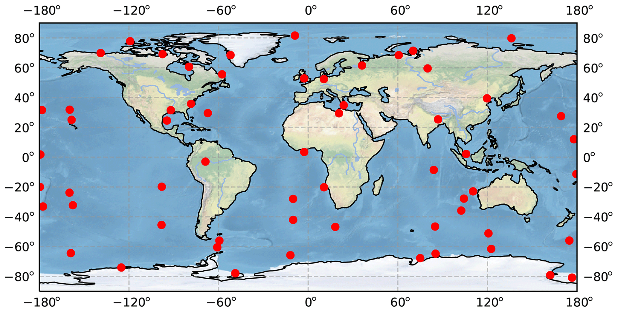
Figure 1Locations of 60 atmospheric profiles with different scenarios.
To ensure sufficient variability in our set of 60 profiles, we have calculated, and illustrated in Fig. 2, the mean (black solid line) plus and minus standard deviation (shaded area) and the minimum and maximum values (black dashed line) of the temperature (a), humidity (b) and ozone (c) profiles. There is significant variability that is similar to that obtained with the profiles in the database available in the RTTOV RTM (Chevallier et al., 2006).
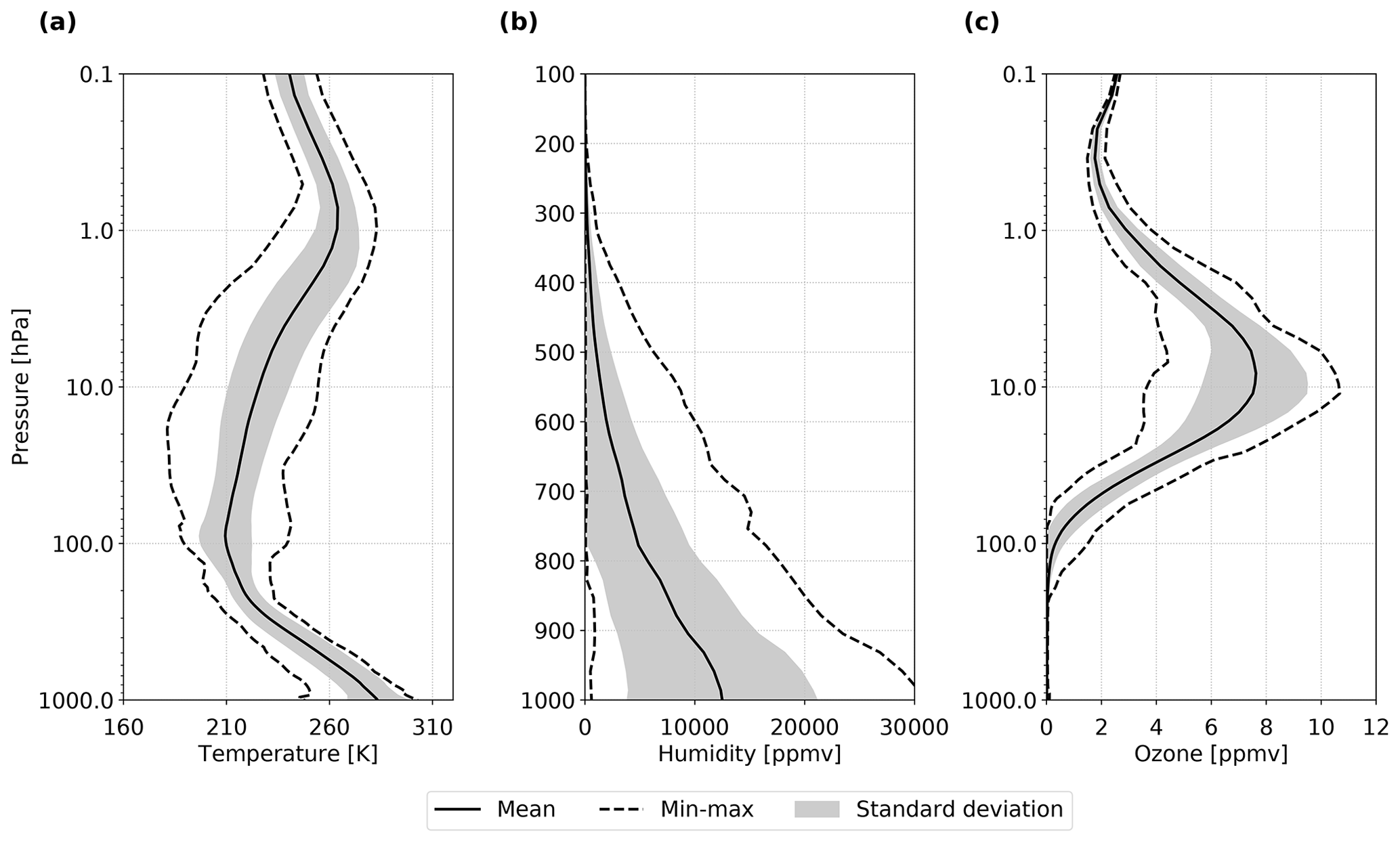
Figure 2Mean ± standard deviation and min–max values of temperature (a), humidity (b) and ozone (c) profile with respect to pressure over the subset of the 60 atmospheric profiles. Note that humidity statistics are shown between 1000 and 100 hPa.
2.2 Channel selection method
The selection of IASI channels made in this study is intended to benefit NWP. Thus, we aim to extract from this selection a maximum amount of information in temperature, humidity, ozone and surface temperature. In order to evaluate the ability of the IASI channels to provide information on these parameters, we have chosen the selection method from the degrees of freedom for signal (DFS), which is used to select a set of optimal channels having the largest information content for each atmospheric profile as described by Rodgers (1996, 2000). The DFS is based on information theory and provides a measure of the gain in information gathered by the observations according to the following formula:
where Tr denotes the trace, I the identity matrix, B∈ℝnxn (n parameters to be retrieved) is the background-error covariance matrix and A∈ℝnxn is the analysis-error covariance matrix which is calculated as follow:
where R∈ℝmxm (m channels considered) is the observation-error covariance matrix and H∈ℝmxn (the derivatives of each channel with respect to each parameter) represents the Jacobian matrix for all IASI channels.
In contrast to the channel selection made by Collard (2007), we have chosen not to separate the selection by variables. Thus, in this study, all the channels considered have the ability to provide information on temperature, humidity, ozone and surface temperature at each step of the selection process. Indeed, unlike the selection method chosen by Collard, the use of an R matrix accounting for inter-channel error correlations allows us to consider all the channels sensitive to several variables (temperature from the CO2 band and water vapour, ozone and skin temperature in the atmospheric window). Note that the IASI spectrum is also sensitive to the main absorbing gases (CH4, CO and N2O) and weaker absorbers (CCl4, CFC-11, CFC-12, CFC-14, HNO3, NO2, OCS, NO and SO2). The total DFS taking into account all the information content for these parameters is used as a figure of merit such as
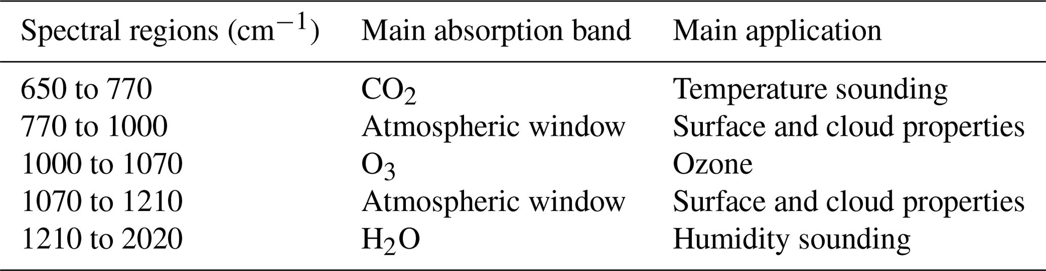
Then, only the first 5499 IASI channels (whose specifications are listed in Table 1) included in band 1 (645 to 1210 cm−1) and 2 (1210 to 2019.75 cm−1) were retained for selection (5500 minus channel 1194 used to retrieve skin temperature). Thus, the channels in band 3 (2020 to 2760 cm−1), influenced by the non-LTE (local thermodynamic equilibrium) effects and the solar irradiance, were not considered. Inter-channel error correlations are considered in this study using a diagnosed observation-error covariance matrix from the 5499 channels of IASI. Finally, in order to ensure the robustness of the channel selection, we considered different scenarios simultaneously by performing the selection on a sample of 60 previously chosen atmospheric profiles.
Table 1Table of IASI spectrum specifications for bands 1 (645 to 1210 cm−1) and 2 (1210 to 2019.75 cm−1).
For each atmospheric profile, the selection begins by selecting the most informative of the 5499 channels using the total DFS with a matrix R of dimension 1×1. Then the first selected channel is fixed and the combination of the two most informative channels is searched for among the (5499−1) channels with a matrix R of dimension 2×2. This operation is repeated iteratively until the required number of channels, or the target value of the total DFS, is reached. Here, the channel selection process is stopped when the improvement resulting from the addition of new channels is relatively small. This choice is subjective.
3.1 Radiative transfer model experiments
In order to calculate the Jacobians and to simulate IASI radiances, we used the RTM RTTOV version 12. RTTOV is developed and maintained by the Satellite Application Facility on Numerical Weather Prediction (NWP SAF) of EUMETSAT. In the RTTOV algorithm, the input atmospheric profiles (temperature, humidity and ozone) are variable and provided by the users, the other constituents, such as CO2, CH4, CO, N2O, etc., can also be provided, but in this case, as in operational NWP, they are assumed to be constant profiles in time and space (depending on the version of the coefficients).
3.1.1 Jacobians calculation
The Jacobian is used to evaluate the sensitivity of a radiance to a physico-chemical parameter. For a specified wavenumber (ν), it represents the sensitivity of the brightness temperature (BT) with respect to a change in a geophysical parameter (X) such as temperature, humidity or ozone in our case. It is expressed by the following relation:
The Jacobian shows to which levels in the atmosphere the BT at a given wavenumber is sensitive, with respect to temperature, humidity or concentrations of the different gases present in our case. To take into account the variability that the sensitivity of the IASI channels can have depending on the atmospheric state, the Jacobians of the 5499 channels were calculated on the 60 atmospheric profiles.

Figure 3Mean of temperature (a), water vapour (b), ozone (c) and skin temperature (d) Jacobians of the first 5499 IASI channels (bands 1 and 2) with respect to pressure over the subset of 60 atmospheric profiles (calculated with RTTOV RTM).
Figure 3 shows the Jacobians sensitive to the averages of temperature (a), water vapour (b), ozone (c) and skin temperature (d) of the 5499 IASI channels with respect to atmospheric pressure. We notice that between 645 and 720 cm−1, IASI channels are mainly sensitive to the temperature from the top of the atmosphere to the lower troposphere. Hence, their usefulness is in atmospheric temperature sounding. There is a slight sensitivity of these channels to ozone in the stratosphere. From 720 to 770 cm−1, the channels are not only sensitive to temperature but also to water vapour in the troposphere. The channels in the atmospheric window between 770 and 1000 cm−1 are, as expected, very sensitive to skin temperature and also sensitive for some of them to temperature and water vapour in the lower troposphere. Then the channels in the ozone absorption band between 1000 and 1070 cm−1 have ozone sensitivities over a large part of the atmosphere with maximum sensitivity in the stratosphere between 100 and 10 hPa. There is a slight sensitivity of these channels to temperature in the stratosphere and lower troposphere, to water vapour in the lower troposphere and to skin temperature for some of them. Then the channels located between 1070 and 1210 cm−1 are mainly sensitive to skin temperature with slight sensitivities to temperature and water vapour in the lower troposphere. Finally, the channels in the absorption band of H2O are mainly sensitive to water vapour and temperature over a large part of the troposphere.
We observe that many channels contain information on several variables. This is particularly true for channels located in the two atmospheric windows, some of which have significant temperature and water vapour sensitivities. The selection of these poly-sensitive channels could be beneficial to NWP by allowing information on temperature, humidity and surface temperature to be extracted within the same channel. However, this assumes that the correlations of inter-channel observation error and background error are correctly taken into account.
3.1.2 Simulated IASI radiances
The first step in calculating the observation error covariance matrix is the estimation of the standard deviations of observation error. These can be deduced from the calculation of first-guess (FG) departure standard deviations, i.e. statistics of the differences between the IASI observations measured and simulated using the RTTOV RTM such as
where y is the observation, xb is the background and ℋ is the observation operator. In order to have a robust statistical representation and to take into account the natural variability, we have simulated, for each of the 6123 profiles, the 5499 channels of IASI.
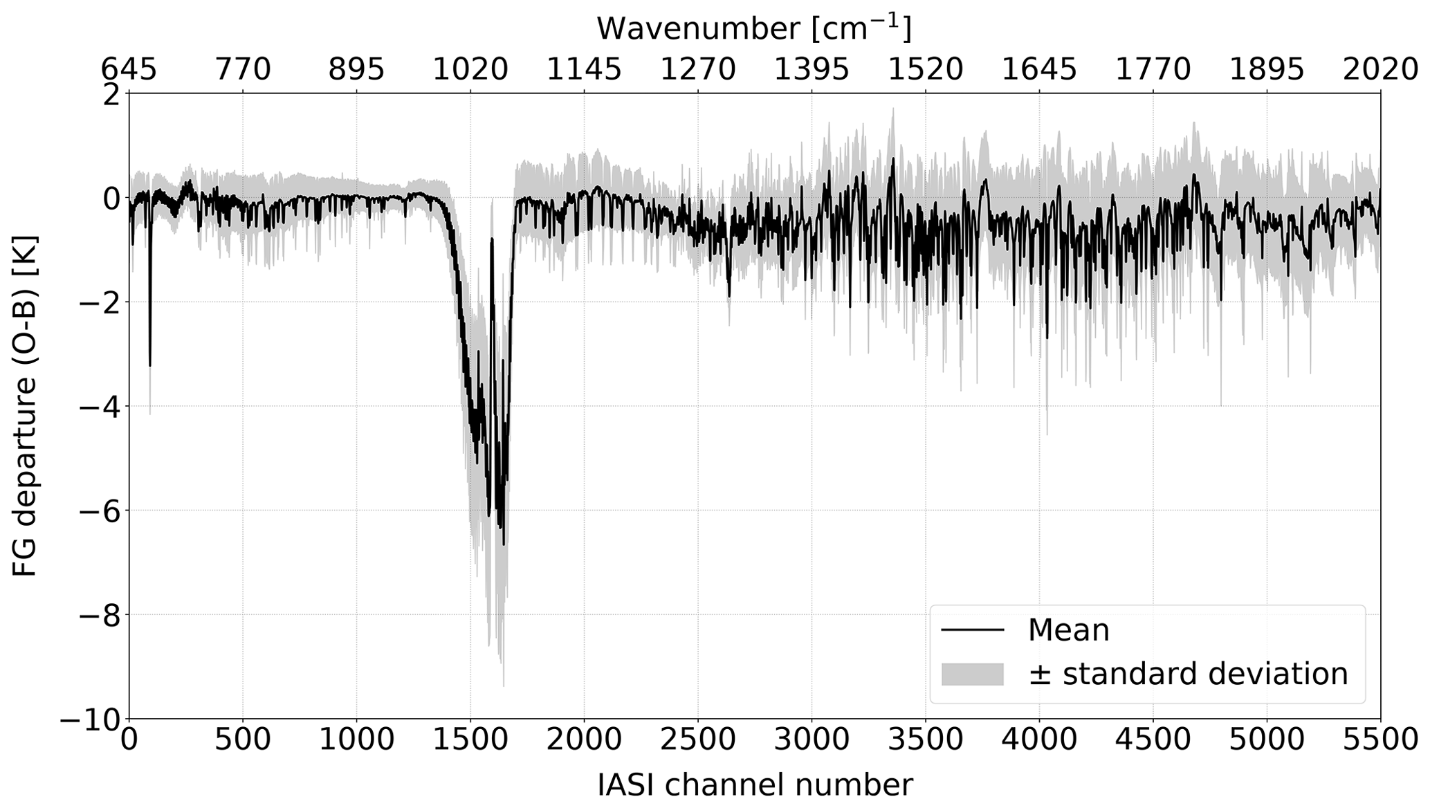
Figure 4Mean ± standard deviation of FG departures with respect to 5499 IASI channel number and wavenumber (cm−1) (bands 1 and 2 without channel 1194) over the set of 6123 atmospheric profiles.
Figure 4 shows the mean (black line) ± standard deviation (shaded) of the innovations with respect to the 5499 IASI channels calculated from the 6123 atmospheric profiles. Note that channel biases between 645 and 770 cm−1 are less than 0.5 K with standard deviations between 0.3 and 0.6 K. The channels of the atmospheric window between 770 and 1000 cm−1 have approximately the same bias values, with biases less than 0.5 K and standard deviations between 0.2 and 0.7 K. The largest values are obtained with the channels in the ozone absorption band between 1000 and 1070 cm−1 with biases between 1.0 and 6.0 K and standard deviations between 0.5 and 2.0 K. These high values are mainly due to the ozone biases found in the MOCAGE CTM. It is able to model the ozone variability correctly but tends to overestimate the ozone concentration (up to 0.75 ppmv) between 300 and 40 hPa and underestimate it (up to 2.5 ppmv) between 30 and 0.1 hPa (Coopmann et al., 2018). These errors in ozone concentrations therefore have a direct impact on the modelling of radiative transfer and on the simulation of IASI channels sensitive to this species. Data assimilation would allow us to correct these biases in ozone; this is currently investigated for the ARPEGE and MOCAGE models. Then, the channels present in the second atmospheric window between 1070 and 1210 cm−1 have biases lower than 0.9 K with standard deviations between 0.5 and 0.8 K. Finally, the channels in the water vapour absorption band have biases of less than 2.0 K and standard deviations between 0.3 and 1.5 K. The higher values of these channels are also due to errors in humidity modelling in the global ARPEGE model. In addition, these abrupt changes from slight to large values are the result of differences in the level of atmospheric sensitivity that may exist between two channels, even if they are spectrally close to each other, which may also lead to differences in the representativeness error.
3.2 Assimilation system
The NWP SAF one-dimensional variational (1D-Var) data assimilation algorithm (Smith, 2016) is based on the optimal estimation method (OEM) (Rodgers, 2000). The unidimensionality makes this algorithm fast, flexible and suitable for research purposes close to NWP operational frameworks. Similar to other variational data assimilation algorithms (e.g. 3D-VAR and 4D-Var), the objective of the 1D-Var is to minimize both the observational and background deviation by minimizing a cost function 𝒥. Assuming that the background error is not correlated to the observation error and the errors have a Gaussian distribution, we retrieve state x by minimizing the cost function such as
where xb is the background profiles, y is the IASI observations, ℋ(x) represents the BTs which are simulated by RTTOV, and B and R are the background- and observation-error covariance matrices, respectively. The retrieved state is called analysis and denoted xa.
In this paper, the 1D-Var algorithm was also used to compute the observation-error covariance matrix from the Desroziers et al. (2005) diagnostic and to evaluate the different channel selections. We modified the code to jointly retrieve temperature, humidity, ozone and surface parameters. The profiles are available on 54 pressure levels from 1050 to 0.005 hPa.
3.3 T, q and O3 background errors
In the same way as the observation-error covariance matrix, it is necessary to estimate accurately the background-error covariance matrix B. Since the ozone background errors are not yet available in the ARPEGE NWP model and the temperature and humidity fields forcing the MOCAGE CTM come from ARPEGE, we have chosen to estimate the background errors of temperature, humidity and ozone together using a statistical method with the MOCAGE model.
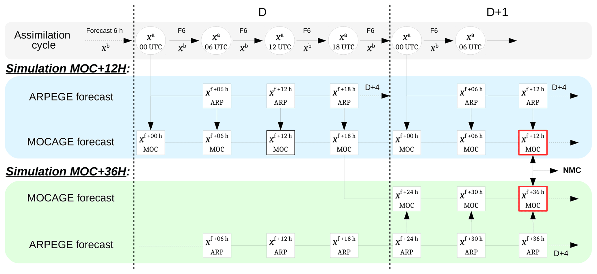
Figure 5 Schematic illustration of the NMC method using MOCAGE CTM, where is the forecast from simulation MOC+12H that is valid at time D. Similarly, is the forecast from simulation MOC+36H that is valid at time D+1.
The National Meteorological Center (NMC) method by Parrish and Derber (1992) is a technique that defines background errors from the difference between NWP forecasts of various ranges valid at the same time. This method is here applied to ozone forecasts. We consider differences from between 36 and 12 h forecast ranges. The background error covariance matrix B is then constructed using long-term modelling results. Two twin simulations were performed. For each one, the configuration uses 60 hybrid levels, from the ground up to 0.1 hPa, and a global domain with a 1∘ horizontal resolution, and the ARPEGE meteorological fields are provided to MOCAGE every 3 h. The model was run from September 2016 to April 2018, with the first 6 months considered spin-up. The various forecasts used in our application of the NMC method are illustrated in Fig. 5:
-
The first simulation uses the operational setup (named here MOC+12H); i.e. every day an ozone forecast up to 24 h is produced by MOCAGE. The initial ozone state of this forecast is the 24 h forecast of the previous day. The meteorological fields used for the forcing of this ozone forecast come from the ARPEGE forecast beginning at the same moment (ARPEGE analysis for 00:00 UTC, then ARPEGE forecasts every 3 h). A 1.5-year simulation has been produced with this cycling mode.
-
In the second simulation (named here MOC+36H), an ozone forecast up to 36 h range is produced. Each day, the ozone forecast is initialized from the MOC+12H ozone initial field valid at the same date. Meteorological forcings are ARPEGE forecasts starting the same day at 00:00 UTC and ranging up to 36 h.
Finally, the B matrix with temperature, humidity and ozone background errors is computed statistically from MOC+12H and MOC+36H forecast differences, valid at the same time, over a 1-year period (March 2017 to March 2018). It should be noted that the ozone background errors estimated here are the result of differences in meteorological forcing from ARPEGE and not chemical differences. Nevertheless, this is a reasonable approximation since the photochemical lifetime of ozone in the upper troposphere and lower stratosphere (UTLS) region is relatively long (Semane et al., 2009). In order to be used in the 1D-Var algorithm, the MOCAGE fields were interpolated on 54 levels from 1050 to 0.005 hPa before calculating the B matrix. As the MOCAGE fields are provided up to 0.1 hPa, the interpolated fields have four levels above 0.1 hPa with similar values. Thus, we have chosen not to use the levels above 0.1 hPa for temperature and ozone background errors. In the same manner, the interpolated fields go up to 1050 hPa, which is in fact rarely reached. We have therefore chosen not to use the first two levels. Finally, as for the B matrix provided by the 1D-Var, we have chosen not to use the levels located in the stratosphere for the humidity background errors.
In conclusion, the 1D-Var experiments and the channel selections will use the temperature (K) and ozone (ppmv) background errors in over 48 levels from 1013 to 0.1 hPa and the humidity background errors (log(kg kg−1)) in over 27 levels from 1013 to 100 hPa. The B matrix was calculated in a multivariate approach, but here we chose to use a univariate B matrix, which means that cross-correlation between temperature, humidity and ozone variables are not taken into account. This assumption prevents feedback effects of ozone on temperature and humidity (Dethof and Holm, 2004).
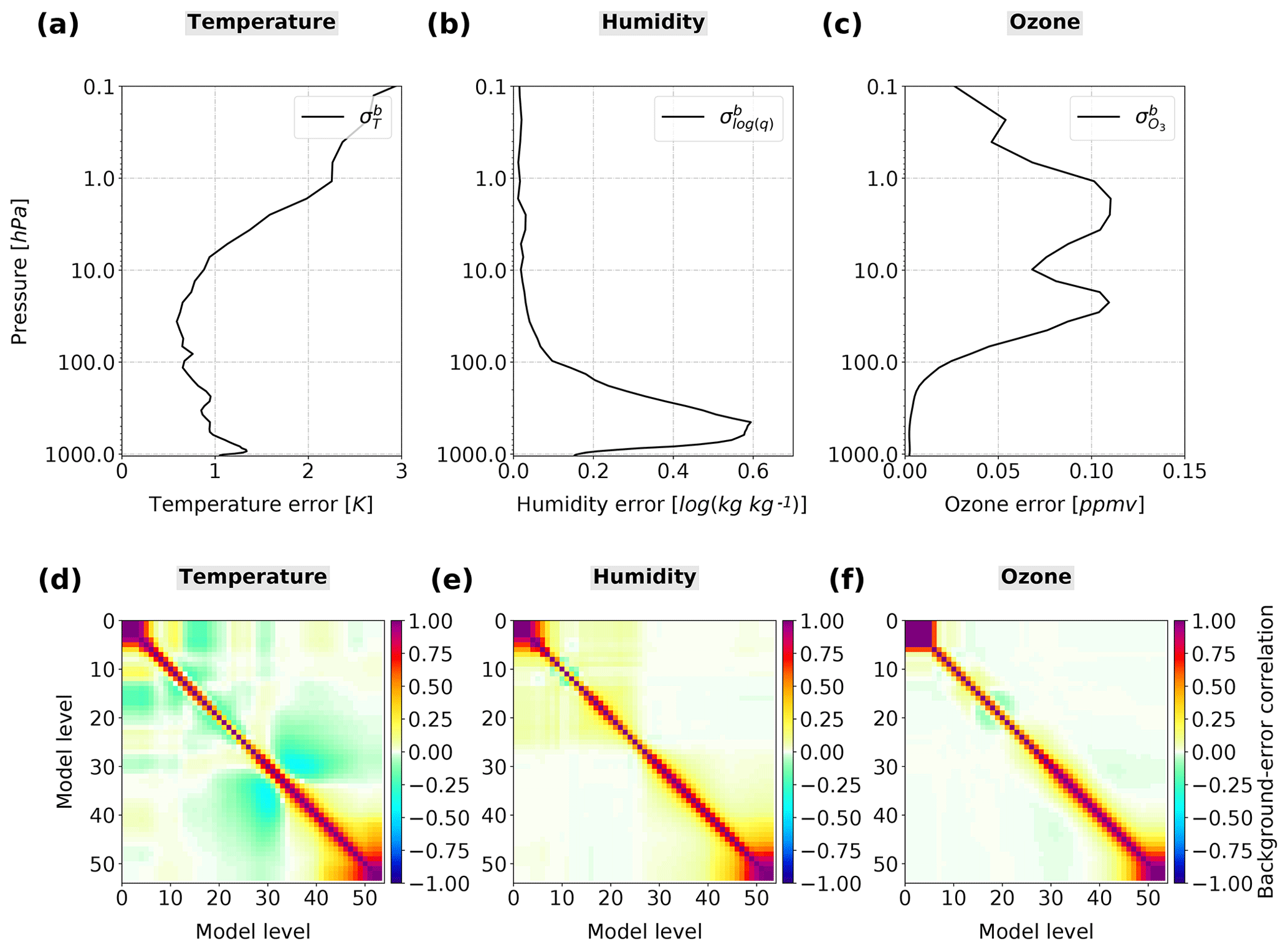
Figure 6Background-error standard deviation of temperature (K) (a), humidity (log(kg kg−1)) (b) and ozone (ppmv) (c) with respect to pressure. Background-error vertical correlation of temperature (d), humidity (e) and ozone (f) with respect to model levels. Note that level 0 is the top model level at 0.005 hPa and level 54 is the lowest model level at 1050 hPa.
We show in Fig. 6 the temperature (Fig. 6a), humidity (Fig. 6b) and ozone (Fig. 6c) background-error standard deviations with respect to pressure, and the temperature (Fig. 6d), humidity (Fig. 6e) and ozone (Fig. 6f) background-error vertical correlations with respect to model levels are also shown. We notice that the correlations for the three variables have higher values in the troposphere between 1013 and 100 hPa (model levels 54 and 25, respectively). Correlations are weaker in the stratosphere and increase in the upper stratosphere, probably due to interpolation as mentioned above. These results for temperature and humidity are consistent with the study carried out by Berre (2000) and Hólm and Kral (2012). Finally, ozone background errors have values up to 0.11 ppmv. This maximum is consistent with values obtained in other studies, e.g. the work by Dragani (2016) and Dragani and McNally (2013), which were carried out using ozone background-error standard deviations with maximum values up to 0.10 ppmv. In addition, the Inness et al. (2015) study for the assimilation of ozone satellite data product (Level 2) into the Composition Integrated Forecasting System (C-IFS) model as part of the Copernicus Atmospheric Monitoring Service (CAMS) programme, used ozone background-error standard deviations with maximum values between 1.4 and 1.6 kg kg−1 or about 0.08 and 0.10 ppmv, respectively. The background errors of skin temperature, surface temperature and surface humidity used in this study are derived from the values available in the reference B matrix of the 1D-Var. The background-error standard deviation value for skin temperature is 2.0 K.
3.4 IASI observation errors
A correct estimation of observation errors is essential in the data assimilation process. Until a few years ago, only the variances of these errors were taken into account (diagonal R matrix). Then innovative techniques to determine these errors and their correlations more accurately by deriving estimates of the real observation error from the departure statistics from assimilation systems emerged to be used for operational NWP (e.g. Hollingsworth and Lönnberg, 1986; Desroziers et al., 2005). Several research works have successfully applied these methods to infrared hyperspectral instruments in order to estimate their total observation errors (instrumental noise, spatial representativeness error, error in the calculation of radiative transfer, etc.). For IASI, many NWP centres are starting to use R matrices that take into account cross-channel error correlations with significant benefits in terms of forecast impact. This is the case at the Met Office (Stewart et al., 2014; Weston et al., 2014), the Environment and Climate Change Canada (Heilliette and Garand, 2015), Météo-France (Vincent Guidard, personal communication, 2019) and the European Centre for Medium-Range Weather Forecasts (ECMWF) (Bormann et al., 2016).
However, these observation errors have been estimated for already selected IASI channels. Considering the significance that inter-channel error correlations can have in the data assimilation process, they should also have a particular influence on the selection of the most informative channels. Some works have consequently carried out new selections of IASI channels using R matrices that take into account inter-channel observation-error correlations (e.g. Migliorini, 2015; Ventress and Dudhia, 2014). They constructed their total R matrix using a “bottom-up” approach (Walker et al., 2011) by estimating separate sources of forward model uncertainty, as opposed to the top-down approach we have chosen to use in this study.
To determine the total R matrix of the 5499 IASI channels for channel selection, we used the following method:
-
First, we constructed a diagonal R matrix with observation-error variances (σo)2 derived from the standard deviations of the innovations previously computed from the simulated observations in RTTOV.
-
Second, we diagnosed the R matrix using the Desroziers et al. (2005) method showing that it is possible to estimate, in observation space, the matrices of background- and observation-error covariances with the deviations of the observations from the background and analysis as
where is the analysis departure and is the first-guess departure. The diagnostic of the R matrix is statistically computed by performing 1D-Var data assimilations on the 6123 profiles.
-
Finally, diagnosing high-dimensional error covariance matrices can lead to estimates that are often degenerate or ill conditioned, making it impossible to invert the matrix. This is precisely the case in this study where the matrix R is diagnosed on 5499 channels and will have to be inverted for channel selection as shown in Eq. (2). Here we have chosen to apply the minimum eigenvalue method to recondition the R matrix. This method has shown its robustness in work by Weston et al. (2014), and Tabeart et al. (2020) concluded that it leads to small overall changes in the correlation matrix, but that it can increase off-diagonal correlations. The consideration of over 6000 profiles for the diagnostic of the R matrix allowed us to recondition the matrix only slightly with very minor changes in the variances and correlations.
Figure 7 shows the observation-error standard deviation from FG departures standard deviation with a red line, diagnosed observation errors with a blue line and instrumental noise of IASI at 280 K with a grey with respect to 5499 IASI channel number (a) and the diagnostic IASI observation error correlation for the same channels (b). The diagnosed observation-error standard deviations are above instrumental noise but below the standard deviations of FG departure. Furthermore, our diagnosed standard deviations of observational error are consistent with those obtained by Bormann et al. (2016) for a subset of channels, except for the ozone-sensitive channels where the ozone background differed from ours. The higher values observed in the ozone and water vapour band for observation-error standard deviations are probably due to errors in the radiative transfer modelling because of larger biases for these variables. Indeed, the ozone profiles from MOCAGE used as an input variable to RTTOV are more realistic than the single profile, but they have biases that can affect the quality of the simulations. Similarly, the humidity profiles from ARPEGE are more realistic in the troposphere than in the stratosphere, which can lead to poor simulations of sensitive water vapour channels in the stratosphere. Hence, this results in these high and low standard deviations in the water vapour band. The values of the observation-error correlations are also consistent with values obtained in other similar studies (Bormann et al., 2016; Migliorini, 2015; Stewart et al., 2014; Weston et al., 2014).

Figure 7Observation-error standard deviation from FG departures standard deviation with a red line, diagnosed observation errors from Desroziers' method using 1D-Var data assimilation system with a blue line and instrumental noise at 280 K in grey with respect to 5499 IASI channel number and wavenumber (cm−1) (bands 1 and 2 without channel 1194) over the set of 6123 atmospheric profiles (a). Diagnostic IASI observation-error correlation with respect to the same channels as before (b).
4.1 Channel selection
Once the matrices R, B and H were determined, we carried out the selection of the most informative channels by solving Eqs. (1) with (3) as the figure of merit. As described in Sect. 2.2, for each of the 60 profiles, we looked for the channel with the highest DFS value, then the channel pair with the highest DFS value, and so on. The selection threshold is achieved when the difference in total DFS between the last selected channel and the previous one is less than 0.005, which corresponds to the 397th selected channel on average over the 60 profiles. We decided to stop our selection at 400 channels for each of the 60 profiles. In Fig. 8, we plotted the evolution of the DFS mean plus and minus standard deviations in temperature (a), humidity (b), ozone (c), skin temperature (d) and total (e) during the IASI channel selection on the subset of 60 atmospheric profiles. A large part of the possible maximum total DFS is reached quickly since 90 % of the maximum total DFS over the 400 channels is achieved with only 172 channels. The maximum skin temperature DFS is obtained very quickly as only three channels are sufficient to provide more than 90 % of the maximum skin temperature DFS over the 400 selected channels. The humidity DFS also increases very quickly. Finally the total DFS with 400 selected channels consists of 50.3 % temperature DFS (7.6), 33.1 % humidity DFS (5.0), 10.1 % ozone DFS (1.5) and 6.5 % skin temperature DFS (1.0).
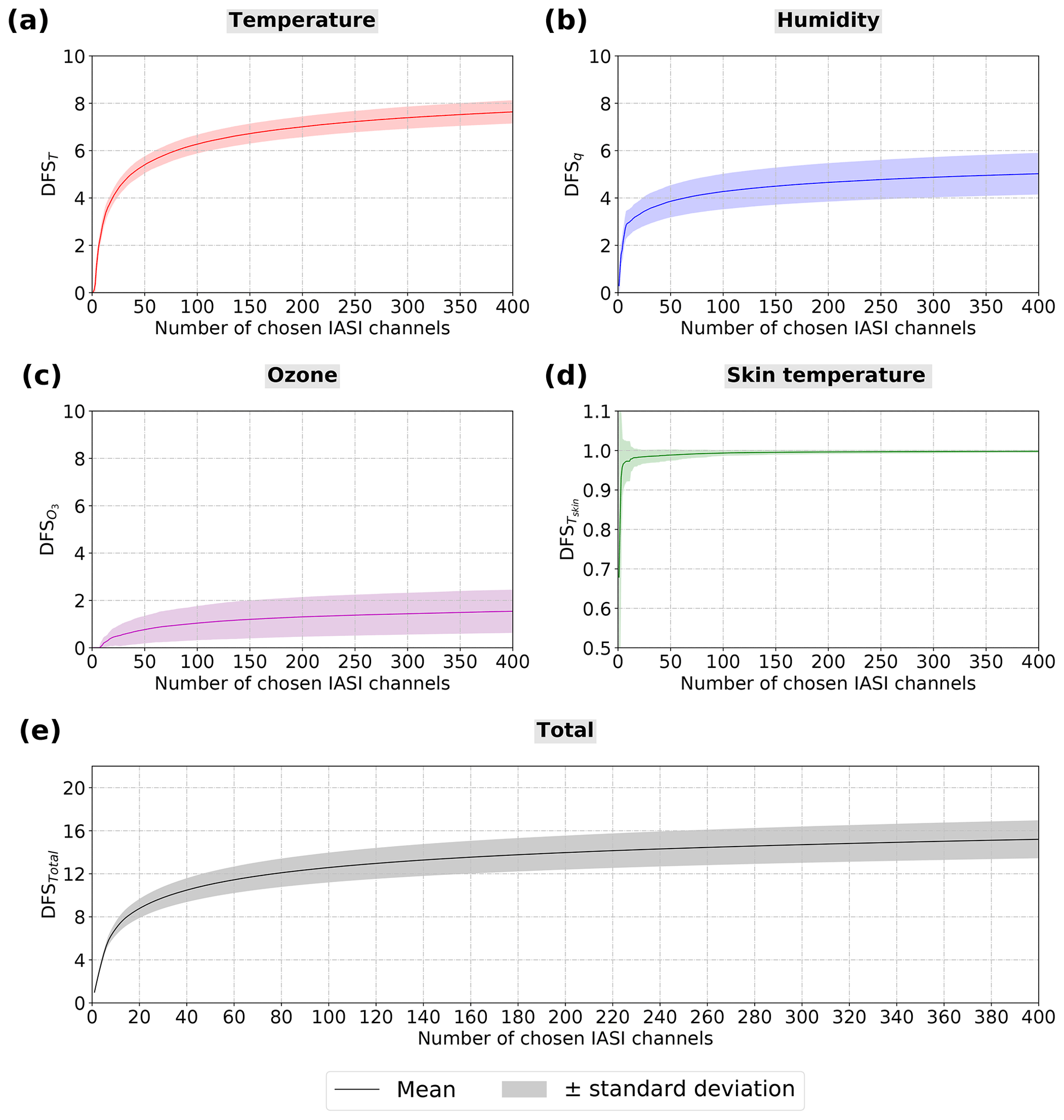
Figure 8Evolution of the mean DFS plus and minus standard deviation for temperature (a), humidity (b), ozone (c), skin temperature (d) and total (e) during the channel selection over the subset of 60 atmospheric profiles.
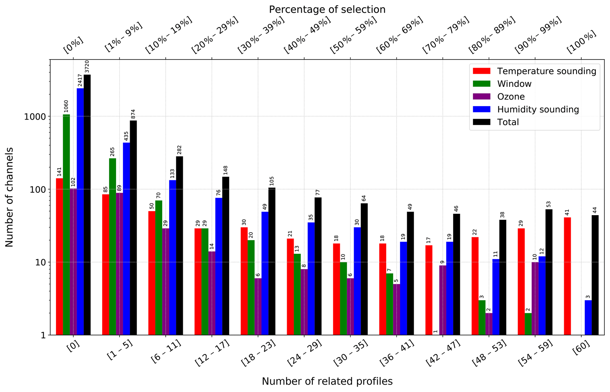
Figure 9Percentage of the number of channels selected (up to 400 channels) on the subset of 60 atmospheric profiles divided by spectral group to temperature sounding (in red), window (in green), ozone (in purple), humidity sounding (in blue) and total (in black).
In order to characterize the channel selection process, a histogram of the percentage of the selected number of channels (up to 400 channels) on the subset of the 60 atmospheric profiles is shown in Fig. 9. These percentages are separated by the main spectral bands to temperature sounding (in red), atmospheric window (in green), ozone (in purple), humidity sounding (in blue) and total (in black). This means that if a channel is selected for all profiles, it achieves 100 % selection. Conversely, a channel never selected among the 60 profiles reaches 0 % selection. In this selection, out of the 5499 available channels only 44 channels are always selected (41 for the temperature sounding and 3 for the humidity sounding) and 3720 channels are never selected, mainly humidity-sounding channels (2417) and channels of the atmospheric window (1060). The channels which are selected more often (>80 %) are mainly temperature-sounding channels. Then humidity-sounding channels are more diversely selected until the end of the process. From these results we can sort the channels selected at least once (1779) according to their selection frequency. Thus the n most frequently selected channels will form a new selection of n channels.
4.2 Comparison
The objective here is to demonstrate that the use of an R matrix accounting for the inter-channel observation errors during the channel selection process allows for more effective identification of the most informative channels compared to a selection using a diagonal R matrix. Therefore, we compared our selection to the channel selection made by Collard (2007) by applying the inter-channel observation errors to it. In this study, we chose not to use the IASI channels in band 3; Collard's selection counts 24 of them. Channel 1194 is excluded for the selection, as it is used for skin temperature retrieval. Which leaves us with 275 channels from the Collard's selection, hereafter named CS275. We have taken the first 275 channels in our new selection, hereafter named NS275.
The first difference between the two selections is that there are less than 30 % of channels in common. Only 60 channels are common in the temperature-sounding spectral group, one in the atmospheric window, 4 in the ozone band and 13 in the humidity-sounding spectral group. This represents a total of 28 % of common channels between CS275 and NS275. It can also be noticed in Table 2 that our selection has more channels in the temperature-sounding and ozone spectral groups and less in the atmospheric window and humidity-sounding spectral groups.
Table 2Spectral band comparison between Collard's and the new channel selection.
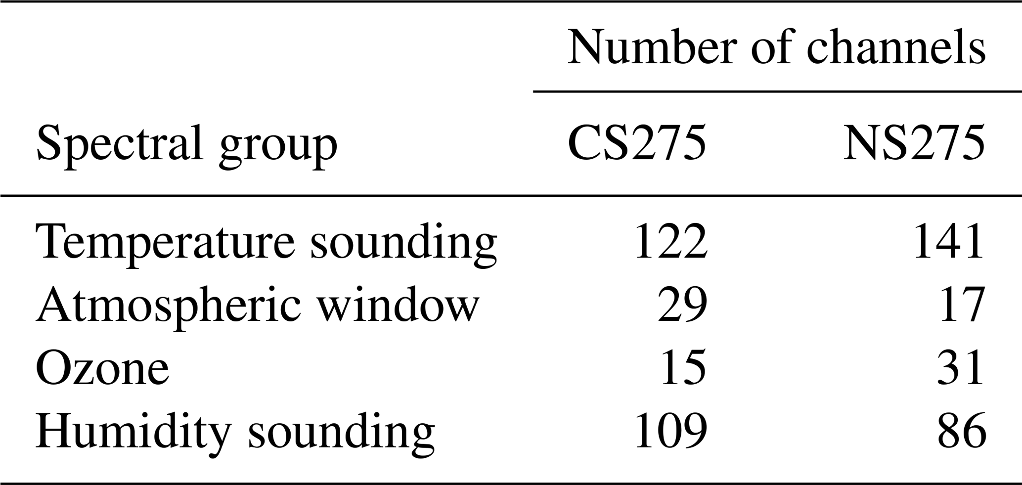
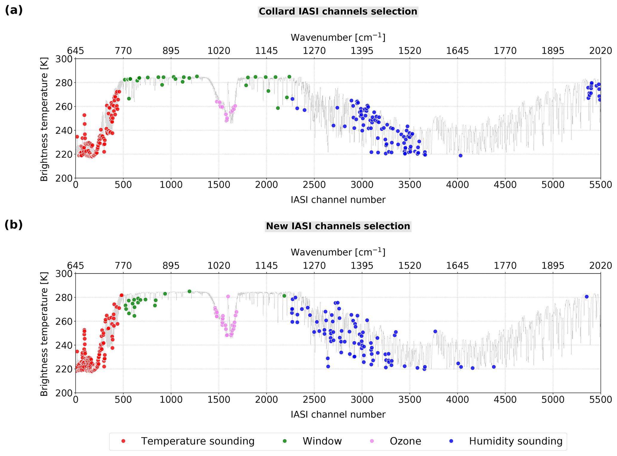
Figure 10Comparison between the 275 channels selected by Collard (a) and the 275 new channels selected (b) on a typical IASI spectrum in brightness temperature on bands 1 and 2. The red, green, purple and blue circles represent the channels of temperature-sounding, window, ozone and humidity-sounding spectral groups, respectively.
The two selections can also be compared in terms of location on the IASI spectrum. In Fig. 10, we have located the selected channels on a typical IASI spectrum in brightness temperature. The red, green, purple and blue circles represent the channels of the temperature-sounding, atmospheric window, ozone and humidity-sounding spectral groups, respectively. Note that NS275 mainly selects channels at the beginning of the spectral bands. Indeed, the channels selected in the atmospheric window are mainly located at the beginning of the first window band. The same is observed with the channels selected for the humidity sounding. More ozone channels are selected and distributed over the entire ozone-sensitive spectral band.
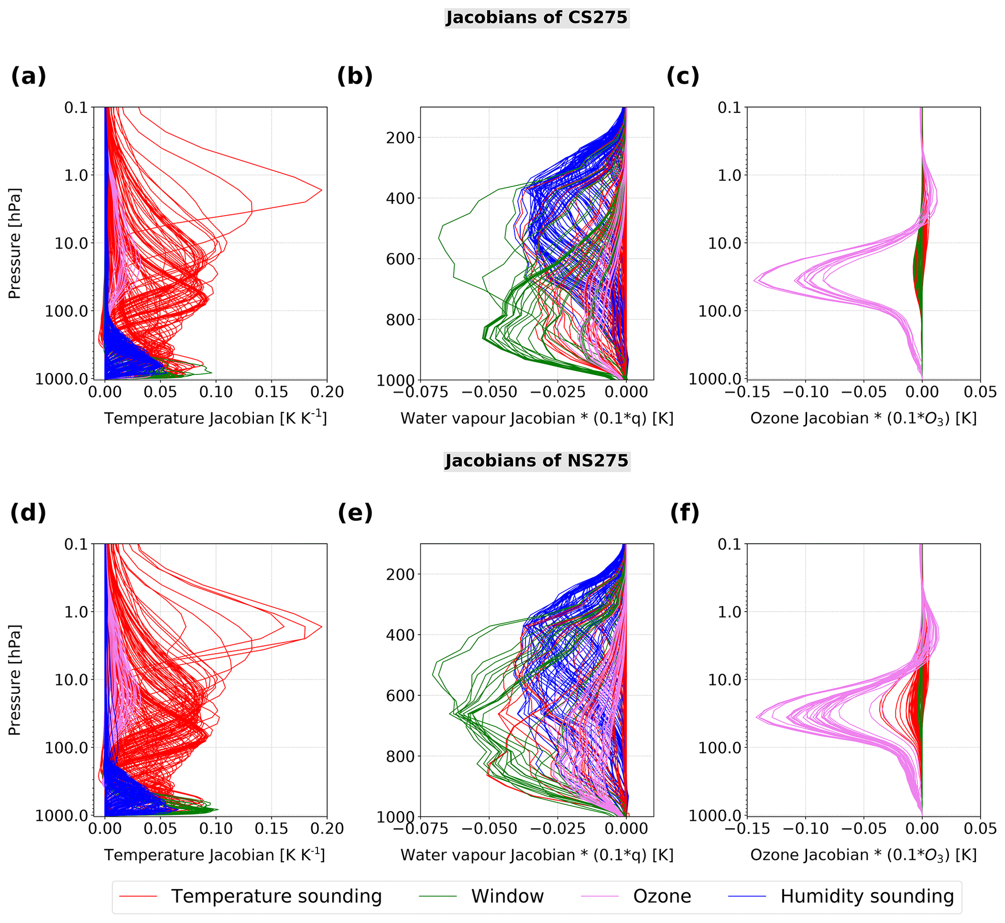
Figure 11Comparison between mean Jacobians of Collard's channel selection (275) for temperature (a), water vapour (b), ozone (c) and mean Jacobians of new channel selection (275) for temperature (d), water vapour (e) and ozone (f). The red, green, purple and blue lines represent the channels sensitive to temperature sounding, window, ozone and humidity sounding, respectively. Note that the water vapour Jacobians (b) and (e) are only shown between 1000 and 100 hPa.
Finally, we compared the Jacobians in the channels of the two selections. We have represented in Fig. 11 mean Jacobians of CS275 for temperature (a), water vapour (b), ozone (c) and mean Jacobians of NS275 for temperature (d), water vapour (e) and ozone (f). The red, green, purple and blue lines represent the channels to temperature sounding, window, ozone and humidity sounding, respectively. The visualization of the Jacobians of the newly selected channels confirms this assumption of channel homogeneity. Indeed, we observe that the temperature Jacobians (d) for the temperature-sounding channels (in red) are relatively evenly distributed especially in the stratosphere for the NS275. We also notice that the temperature Jacobians of the channels selected in the atmospheric window (in green) are higher in the lower troposphere than in CS275. The water vapour Jacobians (e) also show a more homogeneous distribution with the new channels selected mainly there also for the channels in the atmospheric window (in green). The water vapour Jacobians of the ozone (purple) and temperature-sounding channels (red) are also stronger than those of Collard. Finally, as before, the ozone Jacobians (f) have a more homogeneous distribution with the new selection and smaller Jacobian values carried by the temperature-sounding channels (in red). Globally, it is conceivable that this homogeneous distribution of the Jacobians is due to the precise taking into account of inter-channel observation errors during the channel selection process. This allows for the selection of the most informative channels to cover the full range of the atmosphere. Furthermore, we have seen earlier that 90 % of the maximum skin temperature DFS is obtained with only three channels. In addition, Jacobians of the Fig. 3 shows that channels in the first atmospheric window are also sensitive to temperature and water vapour in the lower troposphere. Using these channels could be beneficial to provide additional information for NWP.
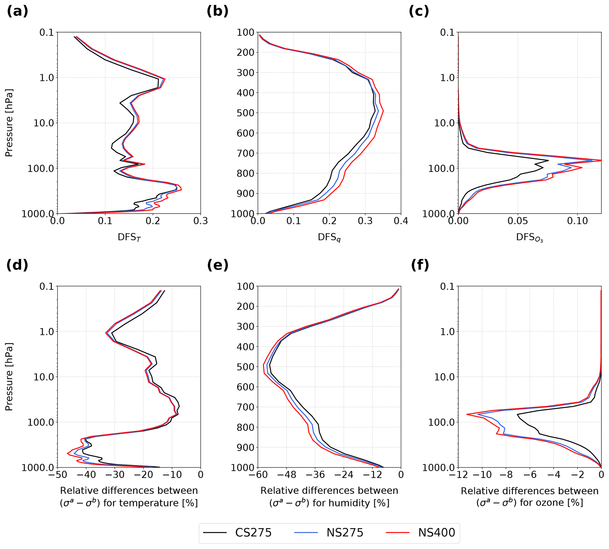
Figure 12 Vertical profiles of mean DFS for temperature (a), humidity (b) and ozone (c) with respect to pressure and vertical profiles of relative difference between analysis-error standard deviation (σa) and background-error standard deviation (σb) for temperature (d), humidity (e) and ozone (f) with respect to pressure. These results are derived from 1D-Var data assimilation experiments over the set of 6123 atmospheric profiles with Collard's channel selection (275) with a black line, the new channel selection (275) with a blue line and the new channel selection (400) with a red line. Note that the vertical profiles of DFSq (b) and relative differences for humidity (e) are shown between 1000 and 100 hPa.
4.3 Evaluation
We evaluated CS275, NS275 and a selection of 400 channels (named NS400) by assimilating them into the 1D-Var (Eq. 6). We used the diagnosed observation error covariance matrices with the appropriate number of channels for each selection. Data assimilation experiments were performed on the 6123 profiles in order to closely approximate the variability of the operational NWP models. In a first step, the DFS mean values of the 6123 profiles for the three selections were calculated. The mean vertical profiles of the DFS for the three selections (Collard in black, the new selection with 275 channels in blue and with 400 channels in red) are shown in Fig. 12 for temperature (a), humidity (b) and ozone (c), and results of DFS values are summarized in Table 3. Compared to CS275 and the equivalent number of channels the NS275 increases the information content since the DFS for temperature is increased by 0.62, for humidity by 0.23 and for ozone by 0.33. It is observed that for temperature, the new selections increase the information content mainly in the stratosphere between 100 and 1.0 hPa and in the lower troposphere between 900 and 300 hPa. For humidity, the information content is increased mainly between 950 and 300 hPa, while for ozone the information content is increased, especially at UTLS. It can be noted that the assimilation of NS400 provides additional information compared to NS275 especially in the troposphere for temperature and humidity and UTLS for ozone.
Table 3Mean of degrees of freedom over 6123 profiles for temperature, humidity, ozone and skin temperature for the three channel selections.

Finally, we evaluated the impact of the different selections by comparing the analysis-error standard deviations (σa) to the background-error standard deviations (σb). Figure 12 shows the mean vertical profiles of the relative differences between σa and σb with respect to the pressure for CS275 in black (d), NS275 in blue (e) and NS400 in red (f). Interestingly, the profiles of DFS and the relative differences between σa and σb are consistent. In addition, NS400 improves everywhere on top of NS275 with additional contribution in the troposphere for temperature and humidity and at the UTLS for ozone.
Table 4Mean of relative differences between analysis-error standard deviations and background-error standard deviations over 6123 profiles for temperature, humidity and ozone for the 3 channel selections.
As expected, the new channel selections further reduce the σa compared to the σb at the same atmospheric levels as previously identified where the information content has been increased. The mean results are summarized in Table 4. We provide a more detailed description of the benefit of the new selections compared to the results with CS275:
-
Compared to CS275, NS275 allows us to reduce on average the temperature analysis error by 3.0 % (3.9 % in troposphere and 1.8 % in stratosphere) with a maximum reduction up to 8.6 % at 700 hPa. Humidity analysis error is reduced by an average of 1.8 % with a maximum reduction of 4.1 % at 745 hPa. Finally, the ozone analysis error is reduced by an average of 0.9 % with a maximum reduction of 3.6 % at 70 hPa.
-
Compared to CS275, NS400 allows us to reduce the temperature analysis error by an average of 4.8 % (6.8 % in troposphere and 2.2 % in stratosphere) with a maximum reduction up to 11.8 % at 700 hPa. The humidity analysis error is reduced by an average of 3.9 % with a maximum reduction of 7.1 % at 750 hPa. Finally, the ozone analysis error is reduced by an average of 1.2 % with a maximum reduction of 4.6 % at 70 hPa.
A new IASI channel selection method was presented in this paper. The objective was to select the most informative channels in the first two spectral bands of IASI between 645 and 2019.75 cm−1 (5499 channels), taking into account the inter-channel observation errors. Indeed, the evolution of the computing capabilities of the weather centres allows them to begin to take into account these error covariances, showing a significant benefit in the use of observations and improvements in weather analysis and forecasts. However, the estimation of these observation-error covariances for IASI is often applied to Collard's channel selection, which was performed using a diagonal R matrix without the inter-channel correlations. Some recent studies have therefore considered the issue of a possible benefit of selecting again the most informative channels of IASI but this time accounting for these inter-channel error correlations. In these studies, the R matrix was estimated using a bottom-up method which represents the R matrix as a sum of random and spectrally correlated components.
The Desroziers et al. (2005) diagnostic is an efficient method to estimate the observation-error covariances accurately. We used this method as a top-down method that uses first guess and analysis departure statistics to diagnose variances and covariances of observation error. It is this method we have chosen to use here to diagnose our R matrix for the 5499 IASI channels considered. We used the 1D-Var data assimilation algorithm to perform assimilation experiments on 6123 atmospheric profiles (and IASI pixels) in order to have a statistically robust sample to diagnose the R matrix and to approximate the possible variabilities that can be found in an operational setting. The diagnosed R matrix provides consistent and satisfying results with other studies on the same subject.
Then, in order to take into account the variability the Jacobians in these channels may have according to atmospheric conditions, we calculated the Jacobians in temperature, humidity, ozone and skin temperature on a subset of 60 profiles selected among the 6123 and representative of the variability of the variables considered. We also constructed a background-error covariance matrix containing the errors of temperature, humidity, ozone and surface parameters. This matrix was computed using the NMC statistical method over 1 year, over the entire globe using the CTM MOCAGE model. The results are still satisfied with errors similar to those used in the weather centres.
A selection of channels using the maximum total DFS (temperature, humidity, ozone and skin temperature) as a figure of merit was made. We chose to stop the channel selection objectively, when the difference in DFS between the last selected channel and the previous one is less than 0.005. This threshold leads to a selection of up to 400 channels. A comparison with Collard's selection (275 channels in bands 1 and 2) showed that our selection of 275 channels has only 28 % of channels in common, and that the newly selected channels are more homogeneously distributed over the IASI spectrum. We also noticed that the new selection uses channels in the atmospheric window that also have sensitivities to temperature and water vapour. The study of the Jacobians of the newly selected channels indeed shows that the channels are better distributed along the atmospheric column and that the channels selected in the atmospheric window have a capacity to provide additional temperature and humidity information.
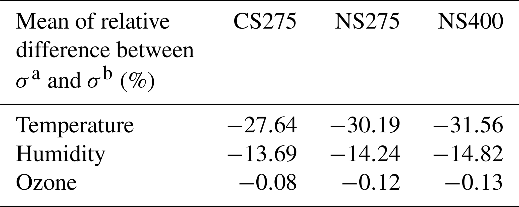
Finally, evaluation of the channel selections using the means of the vertical profiles of the DFS and the means of the vertical profiles of the relative differences between the analysis- and background-error standard deviations shows that for an equivalent number of channels, NS275 reduces the analysis error more than CS275, on average by 3 % in temperature, 1.8 % in humidity and 0.9 % in ozone. Considering NS400, these error reductions can be as high as 4.8 % in temperature, 3.9 % in humidity and 1.2 % in ozone. In this study, we show that NS275 provides additional information on temperature and humidity, especially in the troposphere. It should be noted that some channels selected in this study may be sensitive to minor gases, and others selected between 1210 and 1650 cm−1 may be sensitive to CH4 and N2O. However, none are sensitive to CO (2100–2150 cm−1) since the selection was limited to channels up to 2019.75 cm−1 (more details in Appendix A). The use of inter-channel error correlations exploits the multi-informative potential of the available channels to the atmospheric window and ozone channels.
These results can bring significant improvements in the use of IASI observations by data assimilation systems and be useful for weather forecasting. In the near future, CS275 and NS275 will be evaluated in the 4D-Var data assimilation of the ARPEGE NWP global model and possibly the NS400 selection. The set of 400 selected channels is given in Appendix B.
A sensitivity study was performed to determine the channels of our selection that are sensitive to CH4, N2O and SO2. We performed simulation experiments using the RTTOV radiative transfer model and a database of 83 different variable atmospheric profiles (T, q, O3, CO2, CH4, CO, N2O, SO2) (Matricardi, 2008). We have simulated both perturbed and unperturbed IASI spectra. The profiles were perturbed by the values used in Gambacorta and Barnet (2013), which are 2 % for CH4 and 1 % for N2O and SO2. We calculated the average brightness temperature differences. We considered that channels with a brightness temperature difference greater than 0.01 K are sensitive to the species studied.
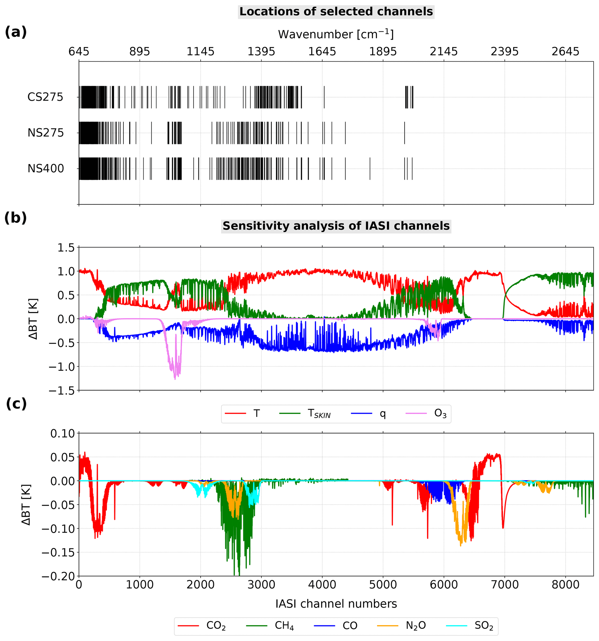
Figure A1Location of CS275, NS275 and NS400 IASI channel selections (a). Sensitivity analysis of IASI channels to temperature, skin temperature, humidity and ozone (b). Sensitivity analysis of IASI channels to carbon dioxide, methane, carbon monoxide, nitrous oxide and sulfur dioxide (c).

The radiative transfer model RTTOV (Saunders et al., 2018) and the unidimensional data assimilation system 1D-Var (Smith, 2016) are developed within the framework of the EUMETSAT Satellite Application Facility on Numerical Weather Prediction (NWP SAF). The partners in NWP SAF are the Met Office, ECMWF, DWD and Météo-France. They are available from the NWP SAF website https://www.nwpsaf.eu/site/software (NWPSAF, 2020).
IASI data are available from EUMETSAT https://www.eumetsat.int (EUMETSAT, 2020). All other data used for this study can be obtained by emailing olivier.coopmann@umr-cnrm.fr.
BJ and VM provided scientific guidance on MOCAGE usage. BJ performed the simulations with the MOCAGE model. The scientific design of the study has been made by OC, VG and NF. OC and VG wrote the codes for the NMC-derived method and the channel selection. OC carried out the channel selection and 1D-VAR evaluation, with significant feedback from VG and NF.
The authors declare that they have no conflict of interest.
The authors would like to acknowledge Jean-François Mahfouf for his help in revising and increasing the quality of the article. This research has been financially supported by CNES and Région Occitanie (PhD grant for Olivier Coopmann).
This paper was edited by Thomas von Clarmann and reviewed by three anonymous referees.
Berre, L.: Estimation of synoptic and mesoscale forecast error covariances in a limited-area model, Mon. Weather Rev., 128, 644–667, 2000. a
Borbas, E. E., Hulley, G., Feltz, M., Knuteson, R., and Hook, S.: The Combined ASTER MODIS Emissivity over Land (CAMEL) Part 1: Methodology and High Spectral Resolution Application, Remote Sensing, 10, 643, https://doi.org/10.3390/rs10040643, 2018. a
Bormann, N., Bonavita, M., Dragani, R., Eresmaa, R., Matricardi, M., and McNally, A.: Enhancing the impact of IASI observations through an updated observation-error covariance matrix, Q. J. Roy. Meteor. Soc., 142, 1767–1780, 2016. a, b, c, d
Boukachaba, N.: Apport des observations satellitaires hyperspectrales infrarouges IASI au-dessus des continents dans le modèle météorologique à échelle convective AROME, PhD thesis, INP Toulouse, available at: http://www.theses.fr/2017INPT0065 (last access: 18 May 2020), 2017. a
Chevallier, F., Di Michele, S., and McNally, A. P.: Diverse profile datasets from the ECMWF 91-level short-range forecasts, European Centre for Medium-Range Weather Forecasts, 2006. a
Collard, A.: On the choice of observation errors for the assimilation of AIRS brightness temperatures: A theoretical study, ECMWF Technical Memoranda, AC/90, 2004. a
Collard, A.: Selection of IASI channels for use in numerical weather prediction, Q. J. Roy. Meteor. Soc., 133, 1977–1991, 2007. a, b, c, d
Collard, A. and McNally, A.: The assimilation of infrared atmospheric sounding interferometer radiances at ECMWF, Quarterly Journal of the Royal Meteorological Society: A journal of the atmospheric sciences, Appl. Meteorol. Phys. Oceanogr., 135, 1044–1058, 2009. a
Coopmann, O., Guidard, V., Fourrié, N., and Plu, M.: Assimilation of IASI ozone-sensitive channels in preparation for an enhanced coupling between Numerical Weather Prediction and Chemistry Transport Models, J. Geophys. Res.-Atmos., 123, 12452–12473, https://doi.org/10.1029/2017JD027901, 2018. a
Courtier, P., Freydier, C., Geleyn, J.-F., Rabier, F., and Rochas, M.: The Arpege project at Meteo France, in: ECMWF Seminar on Numerical Methods in Atmospheric Models, 9–13 September 1991, vol. II, 193–232, ECMWF, Shinfield Park, Reading, available at: https://www.ecmwf.int/node/8798 (last access: 18 May 2020), 1991. a
Courtier, P., Thépaut, J.-N., and Hollingsworth, A.: A strategy for operational implementation of 4D-Var, using an incremental approach, Q. J. Roy. Meteor. Soc., 120, 1367–1387, 1994. a
Desroziers, G., Berre, L., Chapnik, B., and Poli, P.: Diagnosis of observation, background and analysis-error statistics in observation space, Q. J. Roy. Meteorol. Soc., 131, 3385–3396, 2005. a, b, c, d
Dethof, A. and Holm, E.: Ozone assimilation in the ERA-40 reanalysis project, Q. J. Roy. Meteor. Soc., 130, 2851–2872, 2004. a
Dragani, R.: A comparative analysis of UV nadir-backscatter and infrared limb-emission ozone data assimilation, Atmos. Chem. Phys., 16, 8539–8557, https://doi.org/10.5194/acp-16-8539-2016, 2016. a
Dragani, R. and McNally, A.: Operational assimilation of ozone-sensitive infrared radiances at ECMWF, Q. J. Roy. Meteor. Soc., 139, 2068–2080, 2013. a
EUMETSAT: IASI Observations Database, available at: https://www.eumetsat.int, last access: 20 May 2020. a
Fourrié, N. and Thépaut, J.-N.: Evaluation of the AIRS near-real-time channel selection for application to numerical weather prediction, Q. J. Roy. Meteorol. Soc., 129, 2425–2439, 2003. a
Gambacorta, A. and Barnet, C. D.: Methodology and information content of the NOAA NESDIS operational channel selection for the Cross-Track Infrared Sounder (CrIS), IEEE T. Geosci. Remote, 51, 3207–3216, 2013. a
Guidard, V., Fourrié, N., Brousseau, P., and Rabier, F.: Impact of IASI assimilation at global and convective scales and challenges for the assimilation of cloudy scenes, Q. J. Roy. Meteor. Soc., 137, 1975–1987, 2011. a
Heilliette, S. and Garand, L.: Impact of accounting for interchannel error covariances at the Canadian Meteorological Center, in: Proc. 2015 EUMETSAT Meteorological Satellite Conf, p. 8, EUMETSAT, Toulouse, France, available at: https://www.eumetsat.int/website/home/News/ConferencesandEvents/PreviousEvents/DAT_2305526.html (last access: 18 May 2020), 2015. a
Hilton, F., Armante, R., August, T., Barnet, C., Bouchard, A., Camy-Peyret, C., Capelle, V., Clarisse, L., Clerbaux, C., Coheur, P.-F., Collard, A., Crevoisier, C., Dufour, G., Edwards, D., Faijan, F., Fourrié, N., Gambacorta, A., Goldberg, M., Guidard, V., Hurtmans, D., Illingworth, S., Jacquinet-Husson, N., Kerzenmacher, T., Klaes, D., Lavanant, L., Masiello, G., Matricardi, M., McNally, A., Newman, S., Pavelin, E., Payan, S., Péquignot, E., Peyridieu, S., Phulpin, T., Remedios, J., Schlüssel, P., Serio, C., Strow, L., Stubenrauch, C., Taylor, J., Tobin, D., Wolf, W., and Zhou, D.: Hyperspectral Earth observation from IASI: Five years of accomplishments, B. Am. Meteorol. Soc., 93, 347–370, 2012. a
Hollingsworth, A. and Lönnberg, P.: The statistical structure of short-range forecast errors as determined from radiosonde data. Part I: The wind field, Tellus A, 38, 111–136, 1986. a
Hólm, E. V. and Kral, T.: Flow-dependent, geographically varying background error covariances for 1D-VAR applications in MTG-IRS L2 Processing, ECMWF Technical Memoranda, 680, p. 15, https://doi.org/10.21957/3yx4fe6cv, 2012. a
Ide, K., Courtier, P., Ghil, M., and Lorenc, A. C.: Unified Notation for Data Assimilation: Operational, Sequential and Variational (gtSpecial IssueltData Assimilation in Meteology and Oceanography: Theory and Practice), J. Meteorol. Soc. Jpn. Ser. II, 75, 181–189, 1997. a
Inness, A., Blechschmidt, A.-M., Bouarar, I., Chabrillat, S., Crepulja, M., Engelen, R. J., Eskes, H., Flemming, J., Gaudel, A., Hendrick, F., Huijnen, V., Jones, L., Kapsomenakis, J., Katragkou, E., Keppens, A., Langerock, B., de Mazière, M., Melas, D., Parrington, M., Peuch, V. H., Razinger, M., Richter, A., Schultz, M. G., Suttie, M., Thouret, V., Vrekoussis, M., Wagner, A., and Zerefos, C.: Data assimilation of satellite-retrieved ozone, carbon monoxide and nitrogen dioxide with ECMWF's Composition-IFS, Atmos. Chem. Phys., 15, 5275–5303, https://doi.org/10.5194/acp-15-5275-2015, 2015. a
Liu, Z.-Q. and Rabier, F.: The potential of high-density observations for numerical weather prediction: A study with simulated observations, Quarterly Journal of the Royal Meteorological Society: A journal of the atmospheric sciences, Appl. Meteorol. Phys. Oceanogr., 129, 3013–3035, 2003. a
Lorenc, A. C.: Analysis methods for numerical weather prediction, Q. J. Roy. Meteorol. Soc., 112, 1177–1194, 1986. a
Matricardi, M.: The generation of RTTOV regression coefficients for IASI and AIRS using a new profile training set and a new line-by-line database, European Centre for Medium-Range Weather Forecasts, ECMWF, UK, (Tech. Memo., 564, available at: https://www.ecmwf.int/en/elibrary/11040-generation-rttov-regression-coefficientsiasi- and-airs-using-new-profile-training (last access: 20 May 2020), 2008. a
Migliorini, S.: Optimal ensemble-based selection of channels from advanced sounders in the presence of cloud, Mon. Weather Rev., 143, 3754–3773, 2015. a, b, c
NWPSAF: Current Software Packages, available at: https://www.nwpsaf.eu/site/software, last access: 20 May 2020. a
Parrish, D. F. and Derber, J. C.: The National Meteorological Center's spectral statistical-interpolation analysis system, Mon. Weather Rev., 120, 1747–1763, 1992. a
Rabier, F., Järvinen, H., Klinker, E., Mahfouf, J.-F., and Simmons, A.: The ECMWF operational implementation of four-dimensional variational assimilation. I: Experimental results with simplified physics, Q. J. Roy. Meteorol. Soc., 126, 1143–1170, 2000. a
Rabier, F., Fourrié, N., Chafäi, D., and Prunet, P.: Channel selection methods for infrared atmospheric sounding interferometer radiances, Q. J. Roy. Meteorol. Soc., 128, 1011–1027, 2002. a
Rodgers, C. D.: Information content and optimization of high-spectral-resolution measurements, in: Optical spectroscopic techniques and instrumentation for atmospheric and space research II, International Society for Optics and Photonics, vol. 2830, 136–147, 1996. a, b
Rodgers, C. D.: Inverse methods for atmospheric sounding: theory and practice, vol. 2, World Scientific, Oxford, UK, 2000. a, b, c
Saunders, R., Hocking, J., Rundle, D., Rayer, P., Havemann, S., Matricardi, M., Geer, A., Lupu, C., Brunel, P., and Vidot, J.: RTTOV v12 science and validation report, UK Met Office, ECMWF, Météo-France, NWPSAF-MO-TV-41, 78 pp., 2017. a
Saunders, R., Hocking, J., Turner, E., Rayer, P., Rundle, D., Brunel, P., Vidot, J., Roquet, P., Matricardi, M., Geer, A., Bormann, N., and Lupu, C.: An update on the RTTOV fast radiative transfer model (currently at version 12), Geosci. Model Dev., 11, 2717–2737, https://doi.org/10.5194/gmd-11-2717-2018, 2018. a, b
Saunders, R. W. and Kriebel, K. T.: An improved method for detecting clear sky and cloudy radiances from AVHRR data, Int J. Remote Sens., 9, 123–150, 1988. a
Semane, N., Peuch, V.-H., Pradier, S., Desroziers, G., El Amraoui, L., Brousseau, P., Massart, S., Chapnik, B., and Peuch, A.: On the extraction of wind information from the assimilation of ozone profiles in Météo–France 4-D-Var operational NWP suite, Atmos. Chem. Phys., 9, 4855–4867, https://doi.org/10.5194/acp-9-4855-2009, 2009. a
Smith, F.: NWPSAF 1D-Var User Manual, Met Office, Exeter, UK, NWPSAF-MO-UD-032, 2016. a, b
Stewart, L., Dance, S. L., Nichols, N. K., Eyre, J., and Cameron, J.: Estimating interchannel observation-error correlations for IASI radiance data in the Met Office system, Q. J. Roy. Meteor. Soc., 140, 1236–1244, 2014. a, b, c
Stewart, L. M., Dance, S., and Nichols, N.: Correlated observation errors in data assimilation, Int. J. Numer. Meth. Fl., 56, 1521–1527, 2008. a
Tabeart, J. M., Dance, S. L., Lawless, A. S., Nichols, N. K., and Waller, J. A.: Improving the condition number of estimated covariance matrices, Tellus A, 72, 1–19, 2020. a
Ventress, L. and Dudhia, A.: Improving the selection of IASI channels for use in numerical weather prediction, Q. J. Roy. Meteor. Soc., 140, 2111–2118, 2014. a, b
Vincensini, A.: Contribution de IASI à l’estimation des paramètres des surfaces continentales pour la prévision numérique du temps, PhD thesis, École Doctorale Sciences de l'univers, de l'environnement et de l'espace, 2013. a
Walker, J. C., Dudhia, A., and Carboni, E.: An effective method for the detection of trace species demonstrated using the MetOp Infrared Atmospheric Sounding Interferometer, Atmos. Meas. Tech., 4, 1567–1580, https://doi.org/10.5194/amt-4-1567-2011, 2011. a
Weston, P., Bell, W., and Eyre, J.: Accounting for correlated error in the assimilation of high-resolution sounder data, Q. J. Roy. Meteor. Soc., 140, 2420–2429, 2014. a, b, c
- Abstract
- Introduction
- Methodology
- Preparatory work
- Results
- Conclusions and perspectives
- Appendix A: Sensitivity analysis of IASI channels
- Appendix B: List of the selection of the 400 new IASI channels
- Code availability
- Data availability
- Author contributions
- Competing interests
- Acknowledgements
- Review statement
- References