2.1 Telescope focus function

Following Frehlich and Kavaya (1991), the coherent Doppler lidar equation can be expressed as

where SNR is the signal-to-noise ratio, varying as a function of range, R, from the instrument; β^′ is the attenuated backscatter coefficient; η is the detector quantum efficiency; c is the speed of light; E is the beam energy; h is Planck's constant; ν is the optical frequency; B is the receiver bandwidth; and A_e is the effective receiver area.

For a monostatic system emitting a circular Gaussian beam, using a circular aperture, and having matched filters, the effective receiver area is given by Frehlich and Kavaya (1991) and Henderson et al. (2005):

where D is the 1∕e² effective diameter of a Gaussian beam, λ is the laser wavelength, f is the effective focal length of the telescope for the transmitter and receiver, and ρ₀ is a turbulent parameter, also termed transverse field coherence length.

Collecting the range-dependent terms, we obtain a unitless telescope focus function:

which is also termed the coherent responsivity (Frehlich and Kavaya, 1991).

The profile of the attenuated backscatter coefficient is then obtained by rearranging Eq. (1):

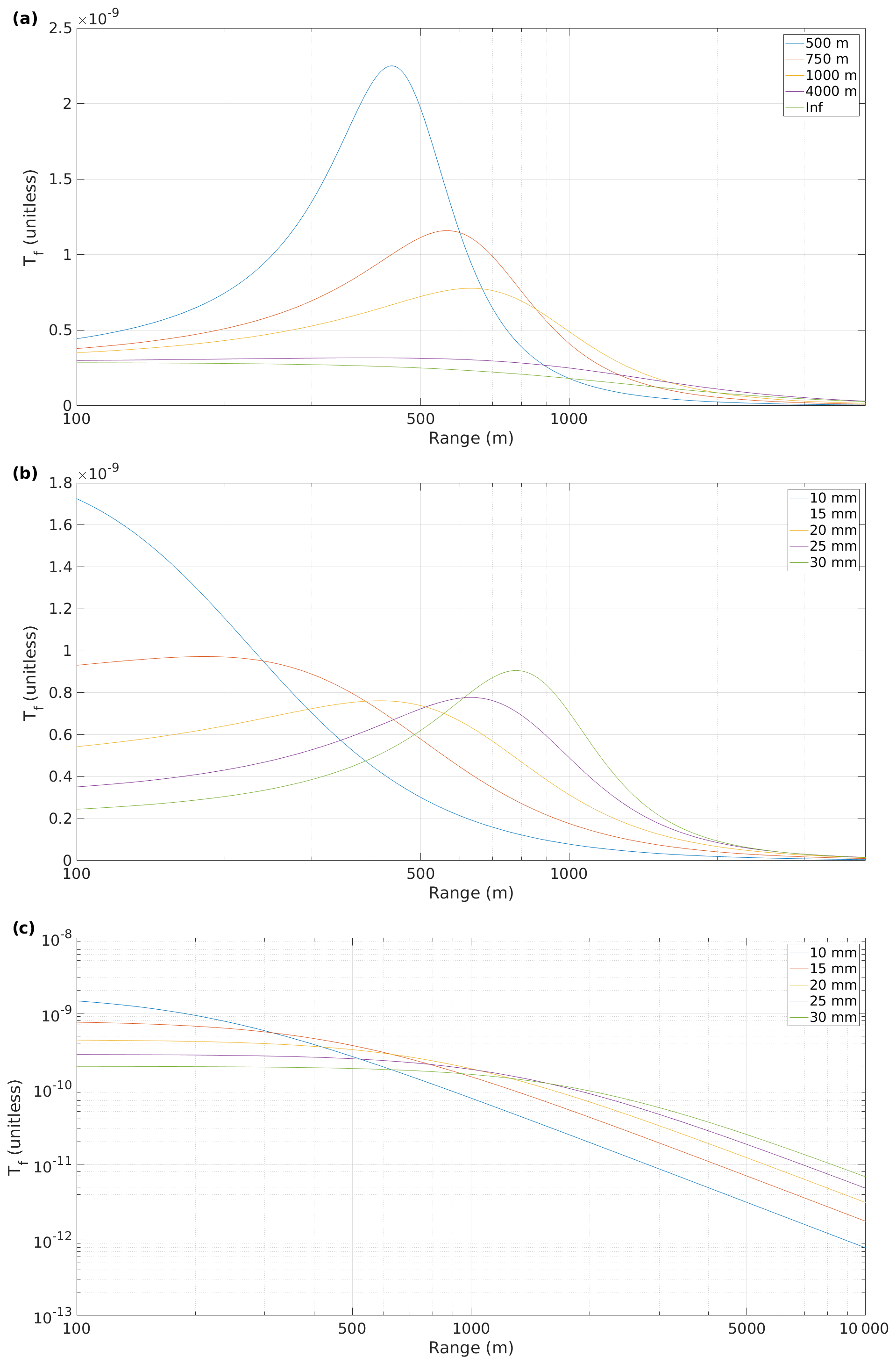
Figure 1Telescope focus functions for (a) varying f with D=70 mm, (b) varying D with f=1000 m, and (c) varying D with f being infinity.

Download

Figure 1a shows how T_f(R) depends on the telescope focal length, f, and Fig. 1b how T_f(R) depends on D. Both figures show that the apparent focus – i.e range to the T_f(R) maximum – is always closer than f and that decreasing D shortens the apparent focus. This makes estimation of the parameters by eye in T_f(R) prone to errors, since the apparent focus cannot be translated into f without knowledge of D.

Figure 1c shows that even if the telescope is focused at infinity, knowledge of the D is essential to derive attenuated backscatter coefficient profiles. While the gradient of T_f(R) may be independent of D at the near and far ranges, the relative magnitude is not, and the potential variation is high in the range of the profile that is commonly of most interest.

2.2 Uncertainty in the attenuated backscatter coefficient

Assuming that the parameters T_f(R) and SNR are independent, and have uncertainties that can be described as Gaussian, the relative random uncertainty in the attenuated backscatter coefficient is

where σ_S is the relative uncertainty in the Doppler lidar SNR, and ${\mathit{\sigma }}_{T_{\mathrm{f}}}$ is the relative uncertainty in T_f(R). An expression for deriving σ_S is given by Manninen et al. (2018), and we describe our method for obtaining ${\mathit{\sigma }}_{T_{\mathrm{f}}}$ in Sect. 4.2.

3.1 Instruments

We used measurements taken from the U.S. Department of Energy Atmospheric Radiation Measurement (ARM, Mather et al., 2016) observatories. We selected five sites with co-located ceilometer and Doppler lidar instruments: Southern Great Plains, US (SGP); tropical west Pacific, Darwin, Australia (Darwin); Barrow, Alaska, US (North Slope of Alaska, NSA); Graciosa, Azores (Graciosa); and Ascension Island, Atlantic, UK (Ascension).

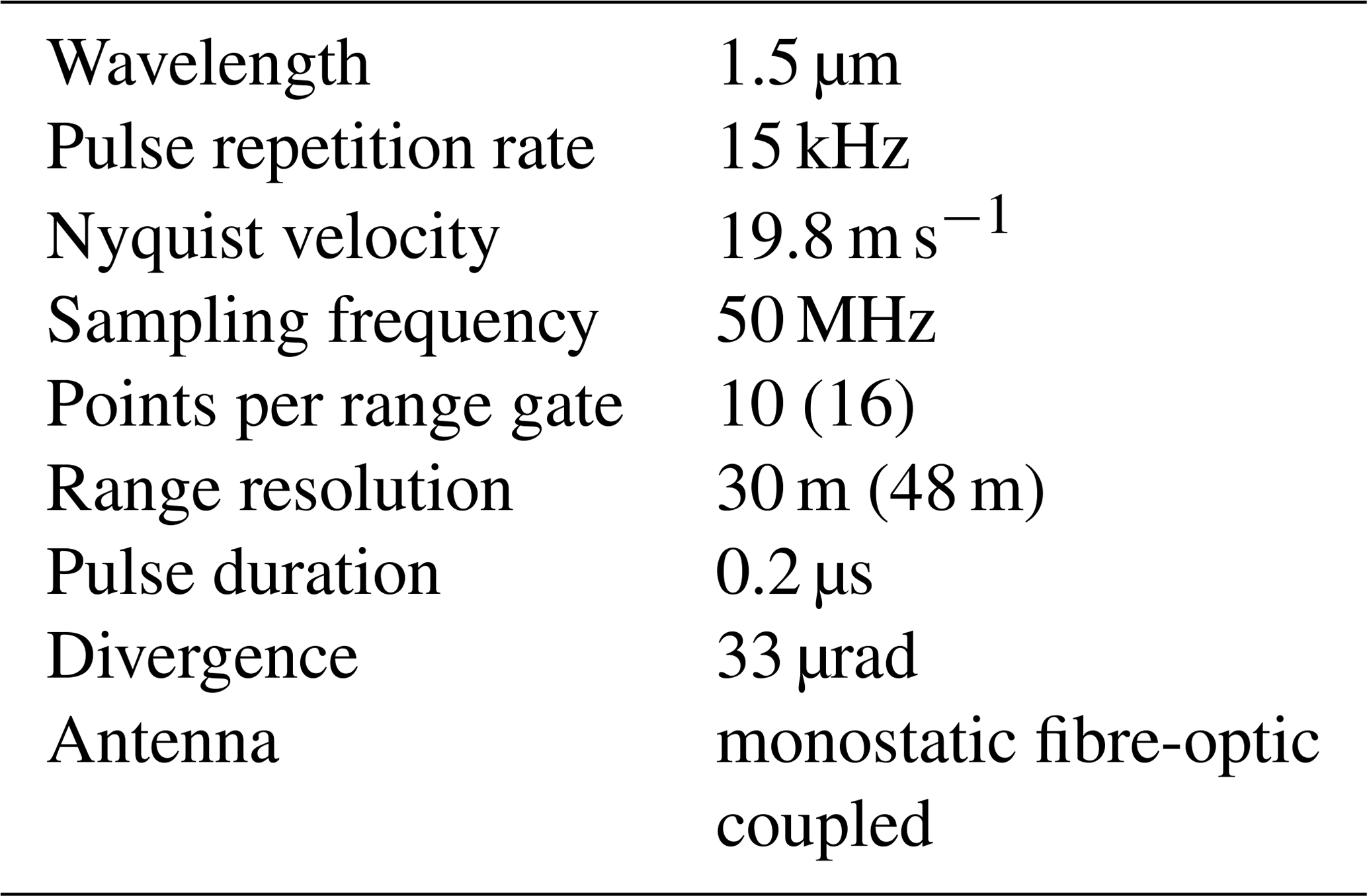
The Doppler lidars operated by ARM comprise both Halo Photonics StreamLine and StreamLine XR versions. These are commercially available heterodyne pulsed systems capable of full hemispheric scanning and operated at a temporal resolution of 1–2 s (see Table 1). The focus for the StreamLine version can be set by the operator, whereas the StreamLine XR has the focus set by the manufacturer; however ARM has had some instruments upgraded from their original specification.

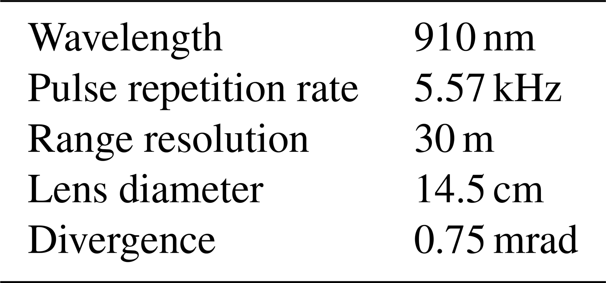
The ceilometer at all sites was a Vaisala CL31 ceilometer, which has a coaxial design and full overlap before 100 m and a temporal resolution of 30 s (more specifications given in Table 2).

Table 1Halo Photonics StreamLine and StreamLine XR heterodyne Doppler lidar specifications. Values in parentheses refer to the specification of the Doppler lidar during the first period in Darwin.

Download Print Version | Download XLSX

Table 2Vaisala CL31 ceilometer specifications.

Download Print Version | Download XLSX

3.2 Methodology

3.2.1 Telescope focus function parameter estimation

The methodology for deriving the parameters of the telescope focus function compares profiles from a co-located Doppler lidar and ceilometer using an iterative least-squares regression to find the best solution. The method follows the process diagram given in Fig. 2.

Figure 2Process diagram of the telescope focus function parameter estimation.

Download

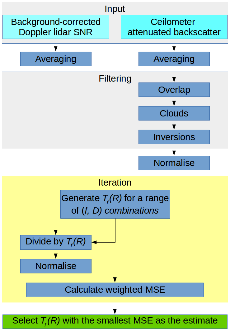
Before input, the Doppler lidar SNR data had a background correction applied to reduce bias (Manninen et al., 2016). Both ceilometer and Doppler lidar data were averaged to a common 30 min, 30 m vertical resolution grid. If the Doppler lidar vertical resolution was larger than 30 m (as was the case for one period from Darwin), linear interpolation was used to match resolutions. After averaging, data below a minimum threshold of −22.2 dB (Manninen et al., 2018) were discarded. The threshold is based on the expected noise floor for the instruments considered here (Halo StreamLine and StreamLine XR) and should probably be modified for different instruments.

The data were then filtered to select only those portions of the profiles that are considered reliable for comparison. Ceilometer data below 195 m were discarded to ensure that only data with full overlap were used.

Due to the wavelength difference between the Doppler lidar and the ceilometer, it cannot be assumed that the atmospheric backscattering properties are the same at both wavelengths. However, we are only interested in the profile shape, not the absolute values, so profiles from the Doppler lidar and the ceilometer can be compared as long as they contain only one type of scatterer, and one which can be assumed to be distributed homogeneously throughout the portion of the profile used for comparison. Hence, the portion of a profile selected for comparison should contain only one aerosol layer, no clouds, and no precipitating hydrometeors.

We removed clouds by identifying the range gate 150 m below the cloud base detected by the ceilometer and excluding all data beyond this. Elevated aerosol layers and precipitating hydrometeors were filtered out by identifying layers using a convolution of the ceilometer profile with a haar-wavelet to detect changes in the gradient. The base of the second layer was identified where the gradient was increasing over two range gates, and all data above this were discarded. This process also eliminates noisy profiles with low SNR.

The T_f(R) parameter estimation is performed on a profile-by-profile basis for each profile where the filtering process leaves eight successive range gates present. From Eq. (4), dividing the Doppler lidar SNR profile with the appropriate T_f(R) will generate a Doppler lidar attenuated backscatter profile whose shape should match that of the ceilometer attenuated backscatter profile.

We use a brute-force approach to iterate through a range of reasonable f and D values, generating a corresponding T_f(R) and Doppler lidar attenuated backscatter profile for each combination of values. The ceilometer profile and resulting Doppler lidar attenuated backscatter profiles are normalised so that the integral value of the unfiltered portion is unity. We then use a least-squares regression using weighted MSE to find the best solution (smallest MSE), where the weights represent the measurement uncertainties in both instruments.

Collecting results over many profiles results in a bivariate distribution; the peak of this distribution is chosen as the best estimate of f and D, and hence the best estimate of T_f(R), using Eq. (3).

3.2.2 Outlier removal

Occasionally, data of poor quality pass the filtering step in Fig. 2. The most common issues are noisy ceilometer data and a bias in the Doppler lidar SNR profiles. If not screened, these occasional profiles result in significantly altered T_f(R) estimation. Any noise in the ceilometer data is magnified by the profile length often being relatively short, and hence large uncertainty in even a single range gate can skew the regression. Doppler lidar SNR bias will impact the normalisation process, changing the T_f(R) selected by the method due to the now incorrect profile shape. Due to the non-linearity of the T_f(R) parameter estimation process, these issues result in regression solutions wildly inconsistent with the estimates based on good data. These outliers, which do not fall within the normal uncertainty observed in good data, are then removed from the bivariate distribution of solutions before calculating the uncertainty estimates.

We used the median absolute deviation, MAD (Huber and Ronchetti, 2009; Leys et al., 2013), to distinguish outliers in the bivariate distribution of estimated f and D. MAD can be calculated using

$$\begin{array}{}\text{(6)}& \mathrm{MAD}=b\mathrm{med}\mathit{\left\{}\right|x_i-\mathrm{med}\mathit{\left\{}{x}_i\mathit{\right\}}\left|\mathit{\right\}},\end{array}$$

where b=1.4826 when the distribution excluding the outliers is normal. However, the distribution of f and D may not meet this criterion due to the non-linearity of T_f(R) and the computational T_f(R) estimation process. We expect the distributions of D and f⁻² to be close to normal and will use f⁻² rather than f to determine outliers. Additionally, the peak of the bivariate distribution may not always coincide with the medians of the univariate D and f⁻² distributions, and, hence, we use a modified form of Eq. (6),

$$\begin{array}{}\text{(7)}& \mathrm{MAD}=b\mathrm{med}\mathit{\left\{}\right|x_i-\mathrm{peak}\mathit{\{}{x}_i,y_i\mathit{\}}\left|\mathit{\right\}}.\end{array}$$

We selected three MADs as the threshold for flagging outliers:

$$\begin{array}{}\text{(8)}& \sqrt{{\left({\displaystyle \frac{f_i^{-\mathrm{2}}-\mathrm{med}\mathit{\left\{}{f}_i^{-\mathrm{2}}\mathit{\right\}}}{{\mathrm{MAD}}_{f^{-\mathrm{2}}}}}\right)}^{\mathrm{2}}+{\left({\displaystyle \frac{D_i-\mathrm{med}\mathit{\left\{}{D}_i\mathit{\right\}}}{{\mathrm{MAD}}_D}}\right)}^{\mathrm{2}}}\ge \mathrm{3}.\end{array}$$

Assuming the distribution excluding the outliers to be normal, three MADs correspond to 3 standard deviations of the underlying distribution. In cases where f is at infinity, all estimates with a finite f will be flagged as outliers.

Table 3Best estimates of f and D together with their uncertainties for Doppler lidars at five ARM sites. Total estimates refers to the number of ceilometer and Doppler lidar profiles suitable for comparison. Good estimates refers to the number of estimates remaining after outlier filtering with MAD.

Download Print Version | Download XLSX

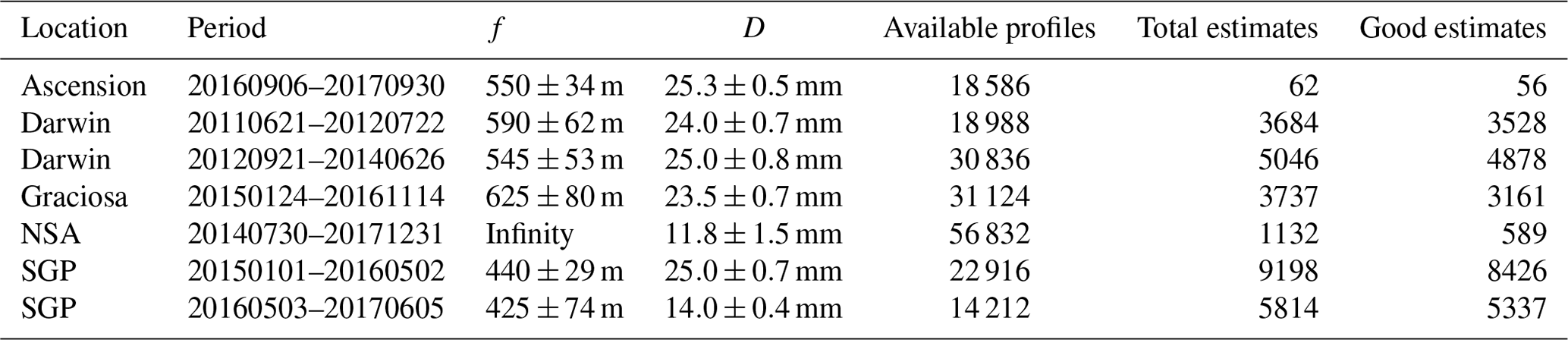
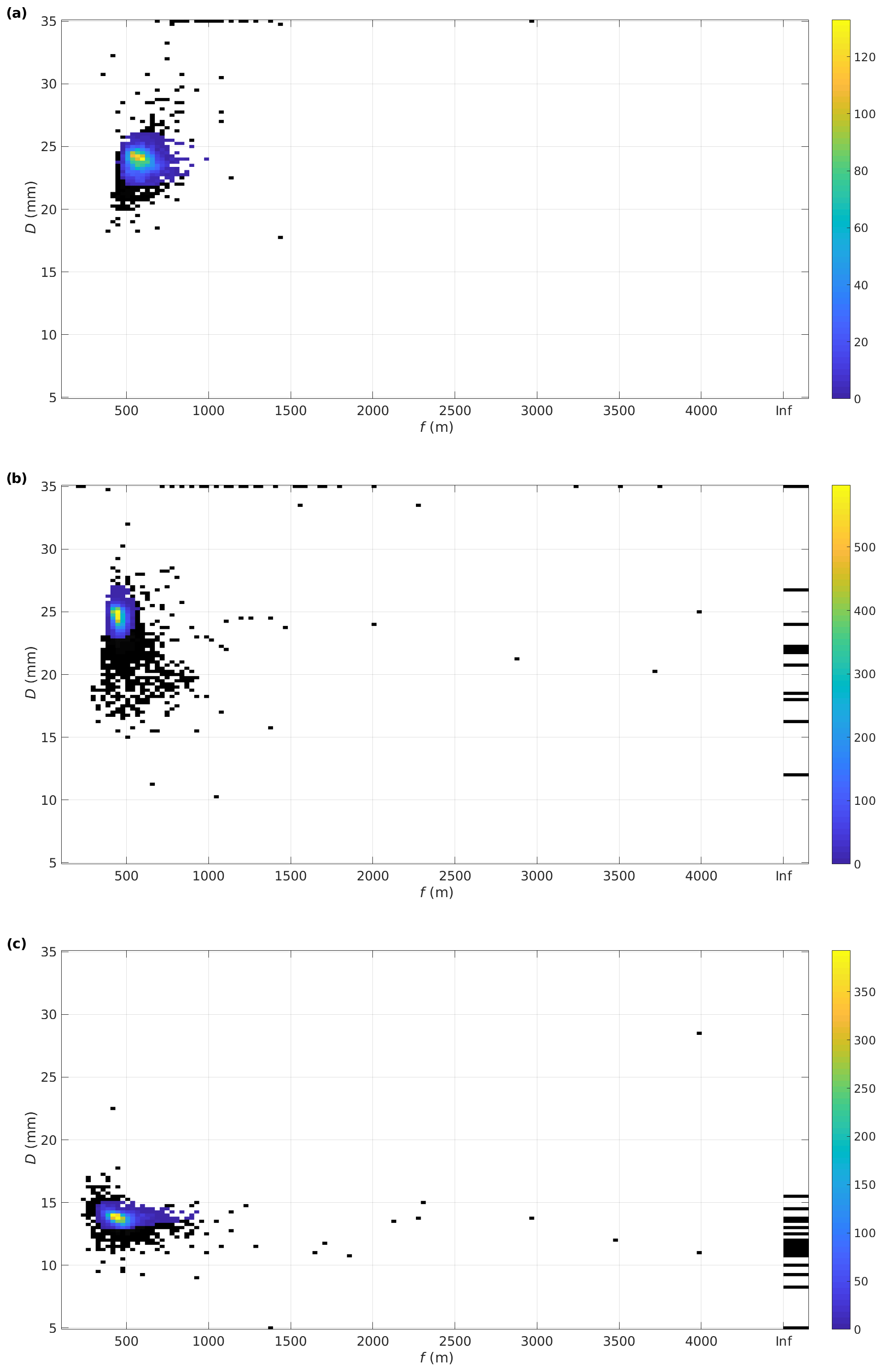
Figure 3Distributions of T_f(R) parameter estimates from (a) Darwin from 21 June 2011 to 22 July 2012, (b) SGP from 1 January 2015 to 2 May 2016, and (c) SGP from 3 May 2016 to 5 June 2017. Outliers filtered using MAD ≥3 are marked in black.

Download

4.1 Parameter estimation

We applied the T_f(R) estimation method to Doppler lidars at five ARM atmospheric observatories. Figure 3a shows the distribution of f and D calculated for the Doppler lidar operating at Darwin in northern Australia between 21 June 2011 and 22 July 2012. This Doppler lidar is a StreamLine and the distribution of f is positively skewed, as explained in Sect. 3.2.2. The distribution displays a slightly wider peak than expected for a normal distribution.

Figure 3b shows the distribution of f and D for the StreamLine Doppler lidar operating at SGP from 1 January 2015 to 2 May 2016. The distribution close to the peak is really tight, while the outliers have substantial spread. Many of the poor estimates responsible for the outlier spread occur during January and February in both years, while for the rest of the period the estimates are remarkably consistent. On 3 May 2016 the Doppler lidar at SGP was changed to a StreamLine XR, and Fig. 3c shows the distribution of f and D from 3 May 2016 to 5 June 2017. The change in instrument version, from StreamLine to StreamLine XR, is clearly seen in the change in D, whereas the best estimate for f did not change. However, inspecting the data by eye would suggest a significantly shorter apparent focus, and the T_f(R) calculated using the best estimates for f and D also exhibits a significantly shorter apparent focus. Consequently, the StreamLine XR in SGP has been noted to suffer from poor SNR at the boundary layer top.

The bivariate distributions of f and D show notable variations in how tight they are around the peak, likely a result of differences in data quality between the instruments. The best estimates of f and D and their uncertainties for all sites are presented in Table 3. The Doppler lidar measurements at Darwin were split into two periods, as there was a 2-month break in the measurements between these two periods. We performed the T_f(R) parameter estimation separately for both periods. The best estimates from these periods differ from each other, which is expected as some adjustments were made to the instrument. The telescope focal length for this instrument is directly adjustable by any operator, while the beam diameter is set by the manufacturer and is not modifiable by the operator. We note that the D estimates are the same for these two periods within the margin of error calculated.

For the sites and instruments selected here, only the Doppler lidar at NSA had f set to infinity. In fact, all StreamLine lidars have D in the vicinity of 25 mm, whereas D for the StreamLine XR versions is about half this. Nevertheless, the variation between instruments of the same version is not negligible and should be taken into account when calculating T_f(R) and then attenuated backscatter.

The final step to obtain attenuated backscatter profiles is to apply a calibration constant, which can be achieved using the liquid cloud calibration method (Westbrook et al., 2010a; O'Connor et al., 2004).

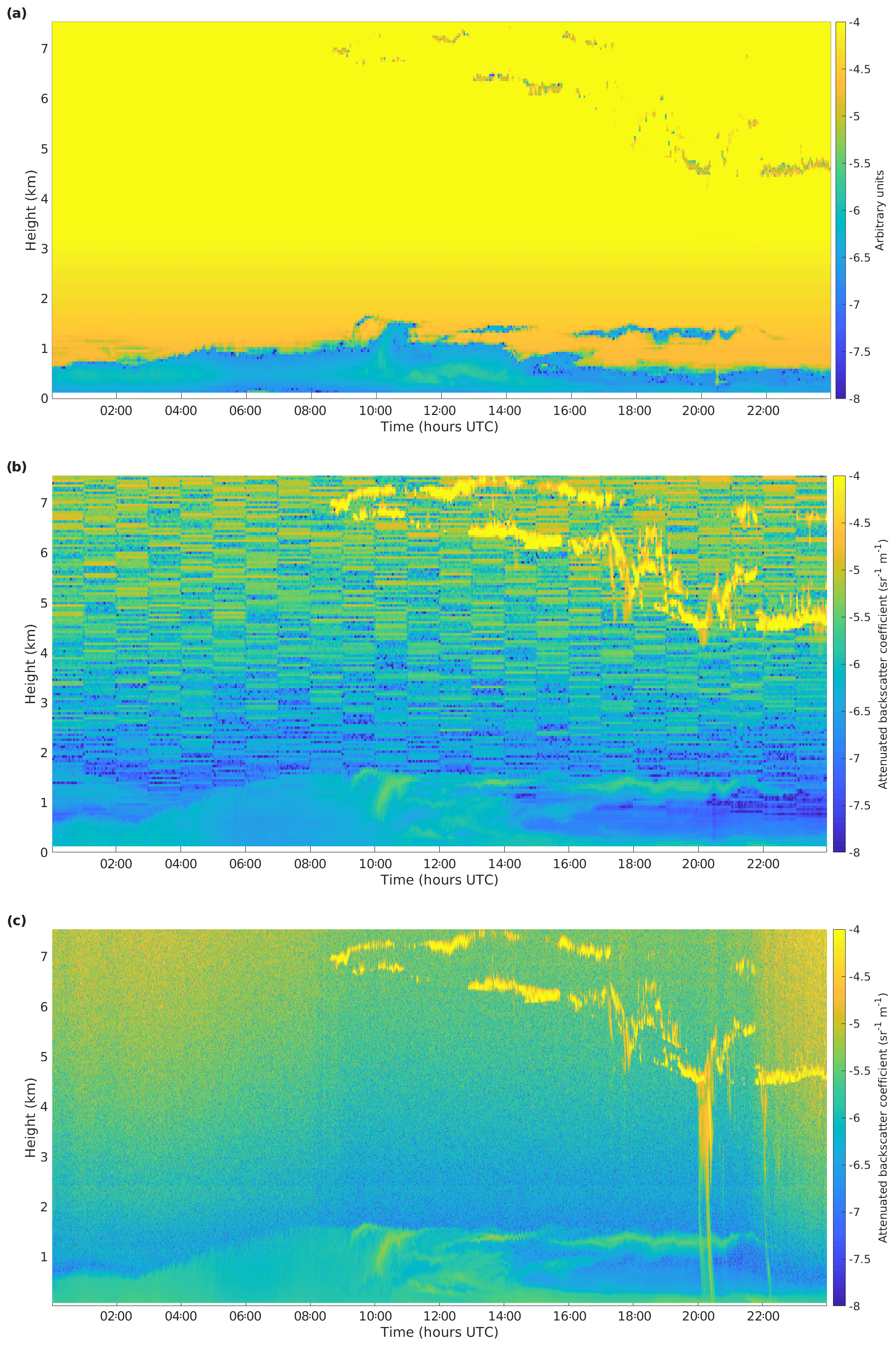
Figure 4(a) Doppler lidar attenuated backscatter coefficient assuming a generic T_f(R), (b) corrected Doppler lidar attenuated backscatter coefficient, and (c) ceilometer attenuated backscatter coefficient, from Darwin on 28 May 2012.

Download

The parameters f and D calculated for period 1 in Darwin have been used to derive T_f(R) and the results applied in Fig. 4. This shows the utility of the method, able to provide reliable Doppler lidar attenuated backscatter profiles in Fig. 4b that show no overcorrection below 1 km and display similar in-cloud values to the ceilometer in Fig. 4c. It is expected that the aerosol attenuated backscatter coefficients will differ due to the different scattering properties of aerosol at the different wavelengths; the scattering properties of cloud droplets remain similar at the two wavelengths (O'Connor et al., 2004; Westbrook et al., 2010a).

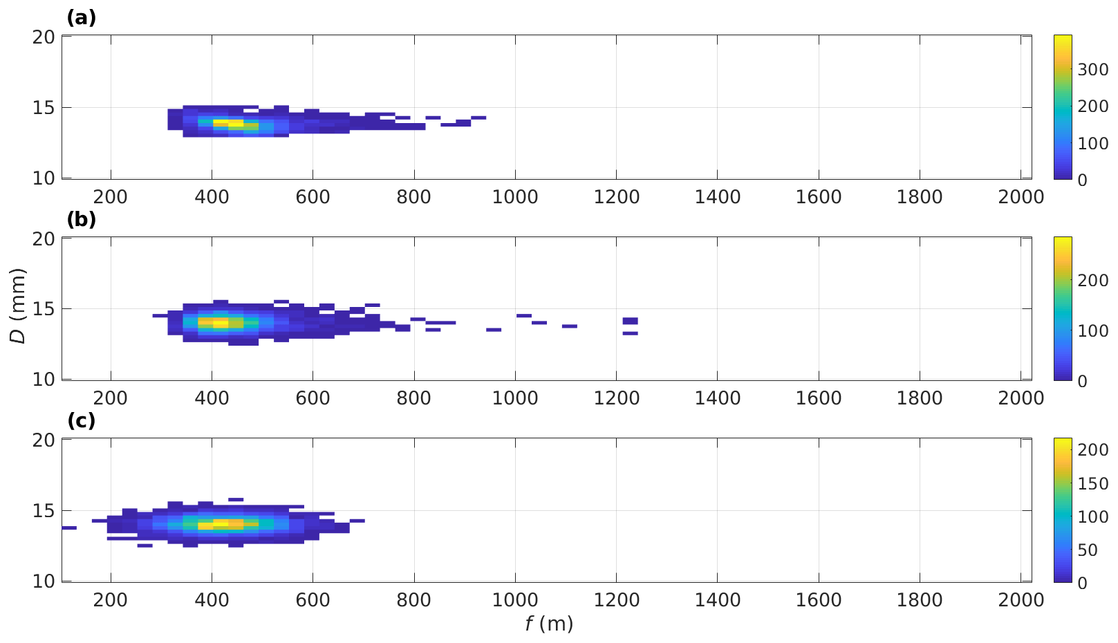
Figure 5Distributions of the Monte Carlo simulation (MCS) input values used for calculating ${\mathit{\sigma }}_{T_{\mathrm{f}}}\left(R\right)$. Values are obtained from (a) resampling, (b) assuming $N(f^{-\mathrm{2}},D)$, and (c) assuming N(f,D). All distributions contain 5337 samples.

Download

Table 4${\mathit{\sigma }}_{T_{\mathrm{f}}}\left(R\right)$ uncertainty envelopes generated using MCS with three different sets of input values.

Download Print Version | Download XLSX

4.2 Uncertainty

A computational method was used to calculate the uncertainty in the estimated T_f(R) as it is a non-linear function of f and D. We used Monte Carlo simulation (MCS) (Morgan and Henrion, 1990), where a distribution of input values is fed into a model, here the effective receiver area Eq. (2), and the uncertainty is obtained from the distribution of the output. The input values can be created either from observed statistics or by bootstrapping, i.e. resampling the data. We created three different sets of input values for our MCS:

1. Resampling the individual estimates of f and D provided directly by the T_f(R) estimation method (i.e. those displayed in Fig. 3) after excluding outliers.

2. Generating the values from the statistics presented in Table 3, assuming that D and f⁻² are normally distributed and independent, $N(f^{-\mathrm{2}},D)$.

3. Generating the values from statistics presented in Table 3, assuming D and f to be normally distributed and independent, N(f,D).

For each set of input values, the relative uncertainty in T_f(R) is calculated as

where ${\mathit{\sigma }}_{T_{\mathit{\varphi }}}\left(R\right)$ is expressed in terms of the mean-squared deviation of the MCS-simulated telescope focus function, T_ϕ(R), from the best estimate of T_f(R),

to avoid underestimating the uncertainty resulting from the asymmetry in T_ϕ(R). This also allows us to estimate the impact of refractive turbulence on the uncertainty estimate.

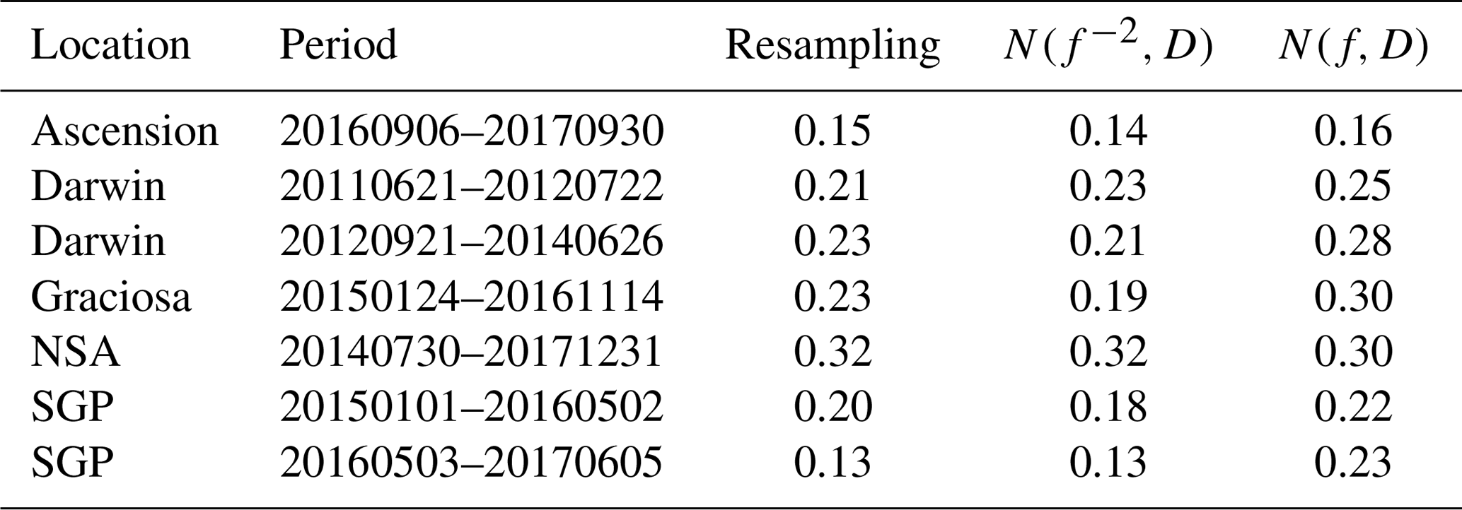
Examples of the three input parameter distributions are presented in Fig. 5. Resampling (Fig. 5a) is the most accurate method as it does not require assumptions about the parameter distributions and their independence. We recommend resampling as the primary method for uncertainty calculation. Using the $N(f^{-\mathrm{2}},D)$ distribution (Fig. 5b) produces a set of input values that appear to be a reasonable approximation, except that the distribution is not as tight around the peak. Using the N(f,D) distribution (Fig. 5c) produces a set of input values that tend to overemphasise shorter values of f and underemphasise higher values. We also note that the central bin of the resampled distribution contains 50 % more samples than the central bin of the statistically generated distributions do. We presume that this is a consequence of the variation in SNR not being necessarily normally distributed.

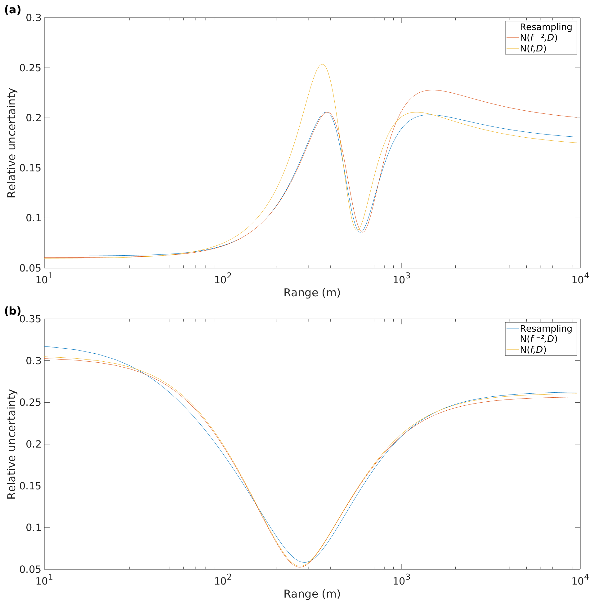
Figure 6Relative telescope focus function uncertainties, ${\mathit{\sigma }}_{T_{\mathrm{f}}}\left(R\right)$, generated using MCS with three different sets of input values for (a) Darwin from 21 June 2011 to 22 July 2012 and (b) NSA from 30 July 2014 to 31 December 2017.

Download

Figure 6a displays ${\mathit{\sigma }}_{T_{\mathrm{f}}}\left(R\right)$ for Darwin showing the range dependence of the uncertainty, with much larger uncertainties for ranges close to either side of the focus (f=590 m). The profile of uncertainties obtained with each set of MCS input values exhibit a similar shape, with $N(f^{-\mathrm{2}},D)$ being closer to resampling than N(f,D) in the near field.

Figure 6b displays ${\mathit{\sigma }}_{T_{\mathrm{f}}}\left(R\right)$ for the Doppler lidar at NSA, which has f set to infinity; therefore ${\mathit{\sigma }}_{T_{\mathrm{f}}}\left(R\right)$ is only dependent on the uncertainty in D. Note the reduced uncertainties around 200–400 m, which are expected when examining Fig. 1c.

The largest value of ${\mathit{\sigma }}_{T_{\mathrm{f}}}\left(R\right)$ provides the uncertainty envelope value for each site, which is presented in Table 4. Resampling provides values ranging from 0.12 for the updated instrument at SGP to 0.32 at NSA. MCS values created using $N(f^{-\mathrm{2}},D)$ provided similar values, whereas MCS using N(f,D) often provided much larger uncertainties.

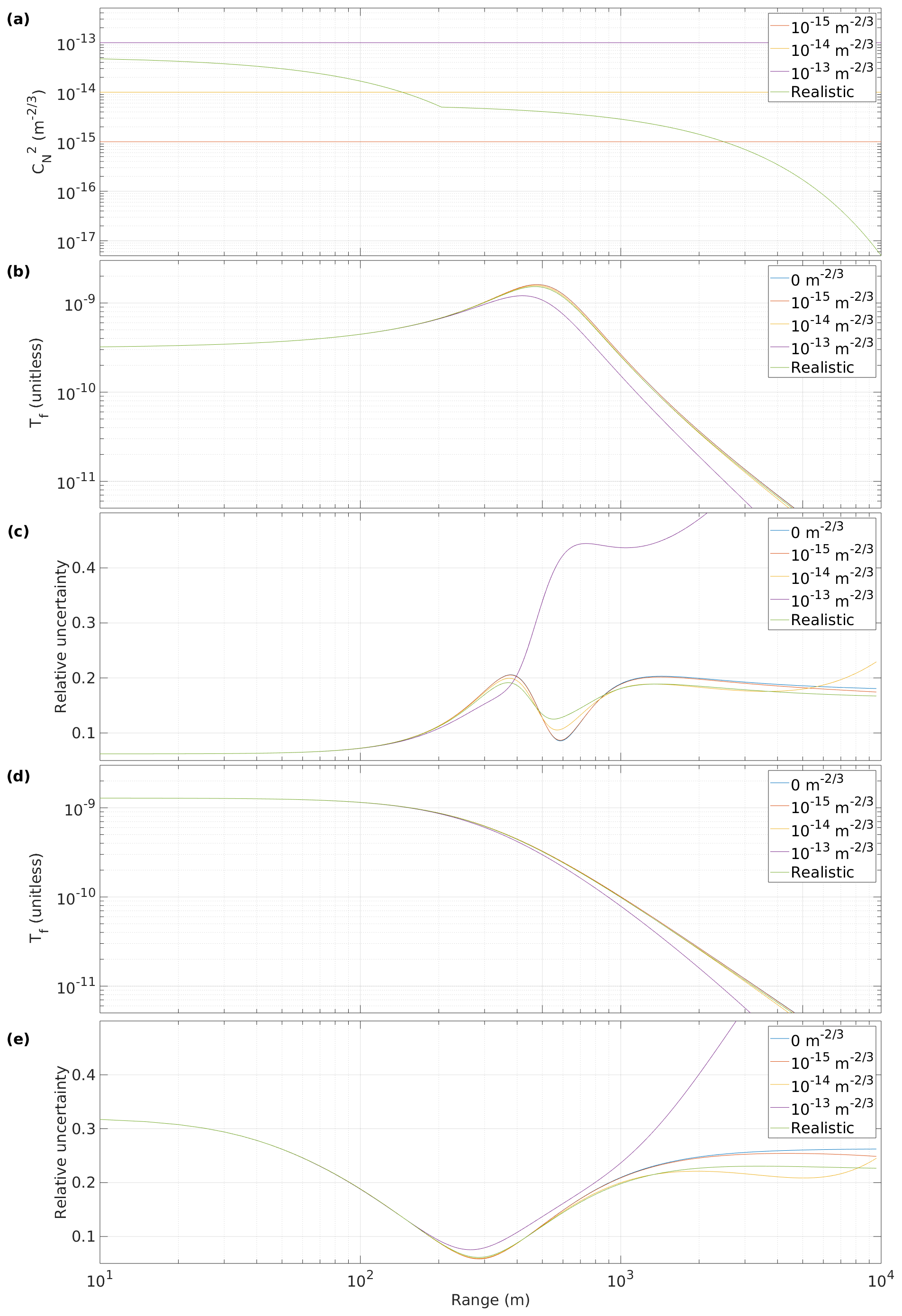
Figure 7Impact of turbulent parameter, ρ₀, on the telescope focus function, T_f(R), and relative uncertainties, ${\mathit{\sigma }}_{T_{\mathrm{f}}}\left(R\right)$, for different ${C_n}^{\mathrm{2}}$ profiles. (a) Selected profiles of ${C_n}^{\mathrm{2}}$ with range; (b) T_f(R) and (c) ${\mathit{\sigma }}_{T_{\mathrm{f}}}\left(R\right)$ for Darwin from 21 June 2011 to 22 July 2012; (d) T_f(R) and (e) ${\mathit{\sigma }}_{T_{\mathrm{f}}}\left(R\right)$ for NSA from 30 July 2014 to 31 December 2017.

Download

4.3 Impact of refractive turbulence

So far we have neglected the potential impact of turbulence on T_f(R) arising from the refractive turbulent parameter, ρ₀, in Eq. (2). An expression for ρ₀ is given in Frehlich and Kavaya (1991),

where H=2.914383, $k=\mathrm{2}\mathit{\pi }/\mathit{\lambda }$, and ${C_n}^{\mathrm{2}}\left(z\right)$ is the refractive turbulence at range z. We chose three profiles with constant ${C_n}^{\mathrm{2}}\left(z\right)$ and a realistic vertical profile based on the most turbulent case presented by Roadcap and Tracy (2009). Figure 7 shows the impact that these different profiles have on T_f(R) and the resulting resampling calculation of ${\mathit{\sigma }}_{T_{\mathrm{f}}}\left(R\right)$ for two Doppler lidar instruments with different T_f(R). Values of ${C_n}^{\mathrm{2}}$ up to ${\mathrm{10}}^{-\mathrm{14}}{\mathrm{m}}^{-\mathrm{2}/\mathrm{3}}$ have negligible impact on T_f(R), and even the realistic profile only showed a slight increase in ${\mathit{\sigma }}_{T_{\mathrm{f}}}\left(R\right)$ for the instrument with a focus set closer than infinity. This suggests that the impact of turbulence can be safely neglected for low values of ${C_n}^{\mathrm{2}}$, and for most applications, it can also be neglected when operating in the vertical. Hence, turbulence has no significant impact on the methodology described here for deriving the parameters f and D and their uncertainties from vertical profiles but can be included for completeness.

However, it is clear that the turbulent impact should not be ignored when measuring at low elevation angles close to the horizon, where a profile similar to ${C_n}^{\mathrm{2}}={\mathrm{10}}^{-\mathrm{13}}{\mathrm{m}}^{-\mathrm{2}/\mathrm{3}}$ may be possible. Figure 7 shows that such a profile has a major impact on T_f(R), especially in the far range. In these cases, the parameters f and D obtained from vertical measurements are still applicable, but ρ₀(R) must also be calculated or estimated in order to derive the profile of attenuated backscatter, β^′(R).

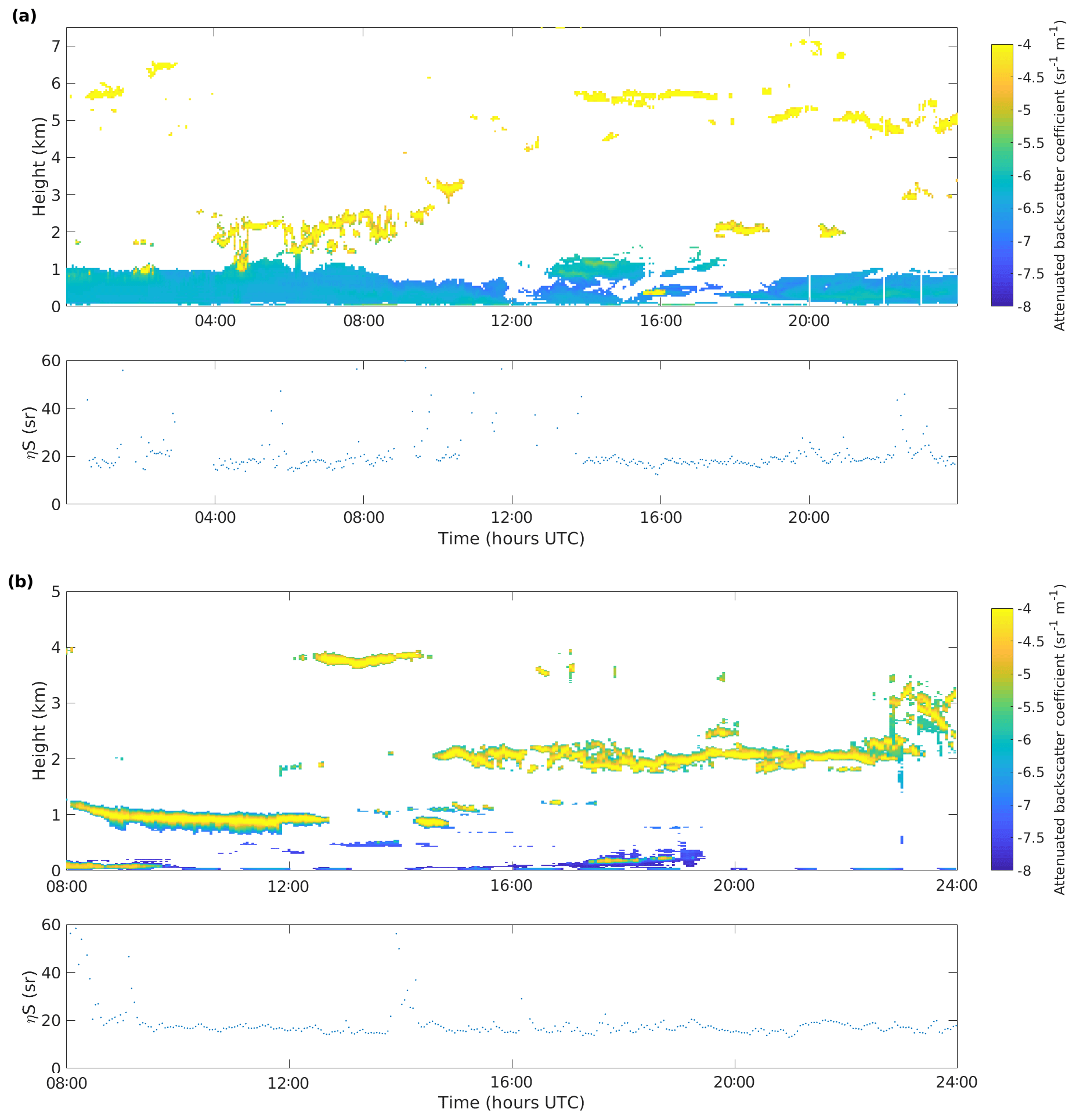
Figure 8Doppler lidar attenuated backscatter coefficient and apparent lidar ratio, ηS, from (a) Darwin on 8 May 2012 and (b) NSA on 20 August 2014.

Download

Limitations

Table 3 shows that the proportion of data that can be used for the T_f(R) parameter estimation varies significantly from site to site. Over a third of the available profiles from SGP are used, whereas only 0.3 % pass the filtering for Ascension. The lack of suitable profiles at Ascension is explained by the almost constant low cloud cover at this site, with very few profiles having a sufficient number of successive range gates.

Data quality is also a limiting factor, so at sites with very low aerosol optical depth, AOD, such as NSA, the Doppler lidar SNR decreases so rapidly that again there are few profiles having a sufficient number of successive range gates. Low AOD also impacts the performance of the ceilometer, with 48 % of the estimates at NSA discarded as outliers even after the initial filtering was performed. While the outlier removal can separate the good and the poor estimates, the largest uncertainty in D was at NSA. We attempted to perform the T_f(R) parameter estimation on a Doppler lidar from an ARM campaign in Cape Cod but could not obtain reliable estimates due to the low SNR of the ceilometer data.

The T_f(R) parameter estimation method is suitable only in situations where there is minimal difference in atmospheric extinction within the aerosol layer between the two instrument wavelengths of 910 and 1500 nm. Using AERONET (Aerosol Robotic Network) AOD measurements co-located at the ARM atmospheric observatories, the median difference in AOD at 870 and 1640 nm varied between 0.016 and 0.027, which should correspond closely to what might be expected for the difference between the ceilometer and Doppler lidar. Very occasional periods of notable AOD differences were observed at some sites, but including these profiles in time series extending beyond a year will have negligible impact on the T_f(R) parameter best estimate. However, there were breaks in the AOD measurements, and some periods experiencing a significant differential extinction may have gone unnoticed. An additional filter using AERONET AOD measurements to remove profiles experiencing significant differential extinction could be included in Fig. 2 for those sites where this may be an issue.