the Creative Commons Attribution 4.0 License.
the Creative Commons Attribution 4.0 License.
 | 16 Jun 2020
Correcting the impact of the isotope composition on the mixing ratio dependency of water vapour isotope measurements with cavity ring-down spectrometers
Alexandra Touzeau
Harald Sodemann
Recent advances in laser spectroscopy enable high-frequency in situ measurements of the isotope composition of water vapour. At low water vapour mixing ratios, however, the measured stable water isotope composition can be substantially affected by a measurement artefact known as the mixing ratio dependency, which is commonly considered independent of the isotope composition. Here we systematically investigate how the mixing ratio dependency, in a range from 500 to 23 000 ppmv of three commercial cavity ring-down spectrometers, is affected by the isotope composition of water vapour. We find that the isotope composition of water vapour has a substantial and systematic impact on the mixing ratio dependency for all three analysers, particularly at mixing ratios below 4000 ppmv. This isotope composition dependency can create a deviation of ±0.5 ‰ and ±6.0 ‰ for δ18O and δD, respectively, at ∼2000 ppmv, resulting in about 2 ‰–3 ‰ deviation for the d-excess. An assessment of the robustness of our findings shows that the overall behaviour is reproducible over up to 2 years for different dry gas supplies, while being independent of the method for generating the water vapour and being the first order of the evaluation sequence. We propose replacing the univariate mixing ratio dependency corrections with a new, combined isotope composition–mixing ratio dependency correction. Using aircraft- and ship-based measurements in an Arctic environment, we illustrate a relevant application of the correction. Based on our findings, we suggest that the dependency on the isotope composition may be primarily related to spectroscopy. Repeatedly characterising the combined isotope composition–mixing ratio dependency of laser spectrometers when performing water vapour measurements at high elevations, on aircraft, or in polar regions appears critical to enable reliable data interpretation in dry environments.
- Article
(3570 KB) -
Supplement
(530 KB) - BibTeX
- EndNote


Stable water isotopes (hydrogen and oxygen) are natural tracers in the atmosphere and hydrosphere and have long been used to improve our understanding of the hydrological cycle and climate processes (Dansgaard, 1953, 1954; Gat, 1996). Advances in laser spectroscopy now allow for high-frequency in situ measurements of the isotope composition of water vapour in the atmosphere (Kerstel, 2004; Kerstel and Gianfrani, 2008). One commercially available type of instrument is the cavity ring-down spectrometer (CRDS) manufactured by Picarro, Inc., USA. The measurement principle of CRDS is based upon the absorption of a laser pulse at a wavelength specific to a given isotopologue (O'Keefe and Deacon, 1988; Crosson, 2008). The Picarro L2130-i and L2140-i CRDS analysers have an optimal performance within a water vapour mixing ratio of 19 000–21 000 ppmv (parts per million by volume), where high signal-to-noise ratios enable precise measurements. This range is typically maintained during liquid sample analysis. In situ measurements of the atmospheric water vapour isotopes are not constrained to this optimal mixing ratio range (Gupta et al., 2009). At lower water vapour mixing ratios, the measurement uncertainty increases due to weaker absorption and, thus, lower signal-to-noise ratios. Additionally, outside of this range, the measurement suffers from a mixing-ratio-dependent deviation of the isotope composition. Since atmospheric mixing ratios can vary from below 500 ppmv in dry regions (e.g. polar regions or the middle and upper troposphere) to 30 000 ppmv or more in humid regions (e.g. the tropics), an appropriate correction for this mixing ratio dependency for high-quality in situ measurements of atmospheric water vapour is required (e.g. Aemisegger et al., 2012; Bonne et al., 2014).
The water vapour mixing ratio dependency (hereafter mixing ratio dependency), sometimes also named the humidity isotope response (Steen-Larsen et al., 2013, 2014) or concentration dependency (Wen et al., 2012; Bailey et al., 2015) of infrared laser spectrometers for water isotopes, has been described in numerous studies (e.g. Lis et al., 2008; Schmidt et al., 2010; Sturm and Knohl, 2010; Bastrikov et al., 2014; Sodemann et al., 2017). Many studies found the mixing ratio dependency to be non-linear and, to some extent, specific to both the instrument used and the isotope composition measured. For example, reviewing the then-available systems for vapour generation on Picarro L1115-i and L1102-i analysers, Wen et al. (2012) showed that the mixing ratio dependency could vary for each specific instrument. Aemisegger et al. (2012) demonstrated that the mixing ratio dependency varies for different instrument types and generations and is affected by the matrix gas used during calibration. However, these authors did not find a substantial dependency on the isotope composition when testing four different standards. Bonne et al. (2014) speculated that the different mixing ratio dependency functions at low mixing ratios (below 2000 ppmv) for their two working standards are likely an artefact of residual water vapour after using a molecular sieve. Bailey et al. (2015) found the mixing ratio dependency to be clearly different for three tested standard waters, while emphasising the uncertainties from statistical fitting in which the characterisation data are infrequent. Sodemann et al. (2017) found a substantial impact from a mixing ratio dependency correction when processing aircraft measurements of d-excess over the Mediterranean Sea but did not account for different isotopic standards in detail. Bonne et al. (2019) characterised the mixing ratio dependency of their ship-based water vapour isotope measurements using four water standards and noted a dependency of the mixing ratio dependency on the isotope standard. They did not observe a significant drift in the dependency for measurements separated by several months. Using the ambient air dried through an Indicating Drierite as a carrier gas, Thurnherr et al. (2020) characterised the mixing ratio dependency for their customised L2130-i analyser operating with two different cavity flow rates. They observed a moderate dependency on the isotope composition with a normal cavity flow rate (∼50 sccm) but found a much weaker, or negligible, dependency on the isotope composition with a high cavity flow rate (∼300 sccm).
To summarise, only some previous studies have recognised the impact of the isotope composition of measured standards on the mixing ratio dependency as a significant uncertainty source. More importantly, no systematic investigation of the influence of the isotope composition on the mixing ratio dependency has been conducted so far. Given the potentially large impact of such corrections at very low water vapour mixing ratios, this is an important piece of research required for enabling the reliable interpretation and comparison of measurements at dry conditions (such as in the high-elevation or polar regions or from research aircraft).
Here we present a systematic analysis of the impact of the isotope composition on the mixing ratio dependency for three commercial CRDS analysers, namely one Picarro L2130-i analyser and two Picarro L2140-i analysers, by using five standard waters with different isotope compositions. Methods and data are presented in Sect. 2. Using the measurements from one analyser, we demonstrate the characterisation of the isotope composition–mixing ratio dependency in Sect. 3. We then evaluate the robustness of the isotope composition–mixing ratio dependency across the three analysers by also considering the different vapour generators, matrix gas compositions, measuring sequences, and temporal stability (Sect. 4). A new correction scheme is proposed in Sect. 5. Using water vapour isotope measurements from aircraft and a ship acquired during the Iceland–Greenland Seas Project (IGP) measurement campaign in the Iceland–Greenland seas (Renfrew et al., 2019) as a test case, we investigate the potential impact of the isotope composition–mixing ratio dependency correction in Sect. 6. We then discuss the potential origin of the influence of isotope composition on the mixing ratio dependency (Sect. 7). Finally, we provide recommendations on how to apply the correction scheme to other analysers (Sect. 8).
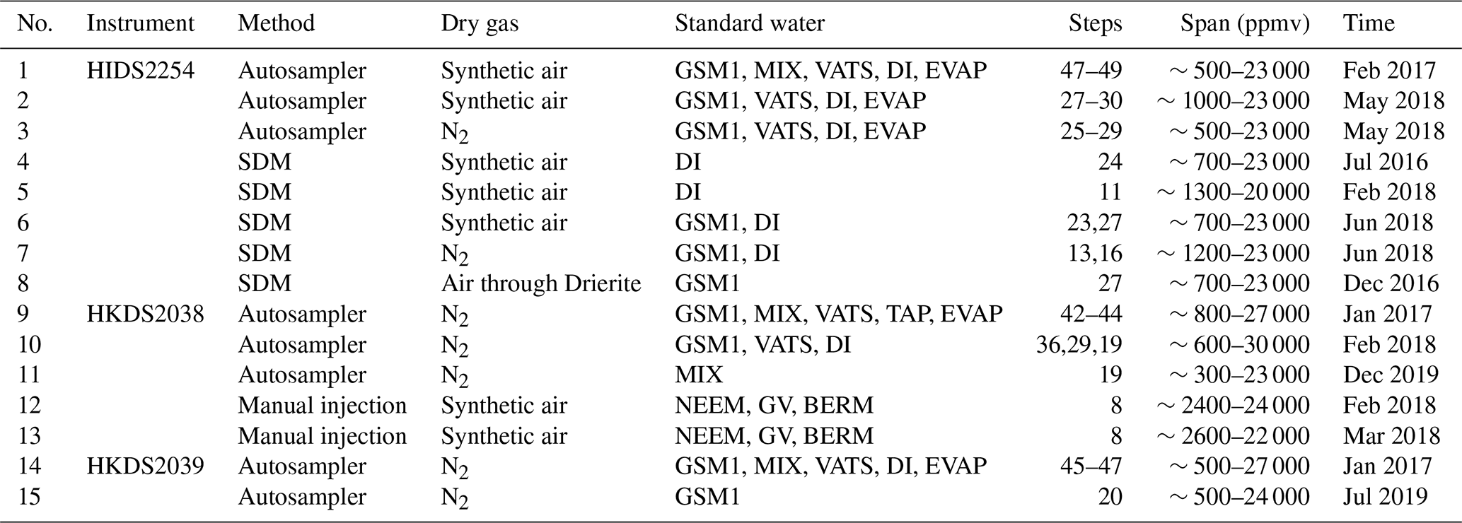
Table 1Overview of all 14 characterisation experiments regarding the instrument, the vapour-generation method, the type of dry gas supply, the measured standard waters, the mixing ratio steps, the mixing ratio span, and the experiment time. For characterisations with injections, four injections are typically carried out at each mixing ratio. For characterisations with continuous vapour streaming via a Standard Delivery Module (SDM), normally 20–40 min of measurements are carried out at each mixing ratio. The values of the water concentrations are the uncalibrated values measured on the corresponding analyser. Instrument HIDS2254 is model type L2130-i, while instruments HKDS2038 and HKDS2039 are of model type L2140-i.
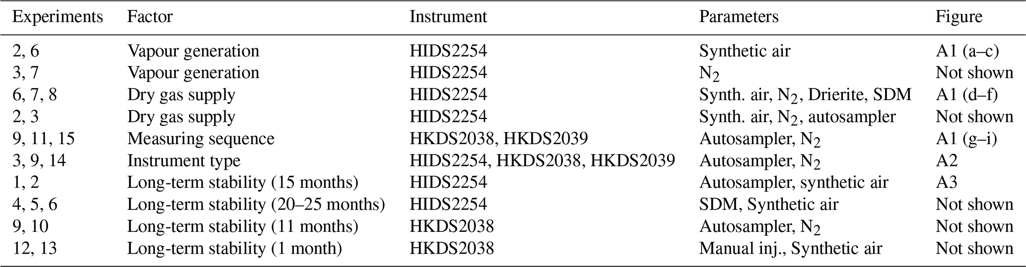
This section introduces the terminology used throughout the paper, explains the measurement principle of the instruments used, and provides an overview of the total of 15 experiments (Table 1) that have been conducted to evaluate the potential influencing factors on the isotope composition–mixing ratio dependency both separately and repeatedly. These 15 experiments can be separated into five categories with respect to their aims (Table 3). With these five categories, we assess the following influencing factors: the dependence on the vapour-generating method, the dependence on the specific instrument, the long-term stability of the dependence behaviour, the influence from the dry gas matrix, and the influence of the measuring sequence. In the end, we introduce the in situ measurement data that are used to illustrate the impact of correction.
2.1 Terminology
The abundance of stable water isotopes in a reservoir is quantified as the concentration ratio of the rare (HD16O or ) to the abundant () isotopologue. Note that the definition here is referred to as the molecular isotope ratio, as measured by laser spectrometry. Apart from statistical factors, this definition can be shown to be equal, in the first order, to the atomic isotope ratio R determined by mass spectrometry (Mook et al., 2001). The (molecular) isotope ratio of hydrogen in a water reservoir, for example, is then as follows:
Isotope abundance is generally reported as a deviation of the isotope ratio of a sample relative to that of a standard, known as δ value, and is commonly expressed in units of per mil (‰) deviation from the Vienna Standard Mean Ocean Water 2 (VSMOW2) by means of (Hagemann et al., 1970) and (Baertschi, 1976). The VSMOW2 is distributed by the International Atomic Energy Agency (International Atomic Energy Agency, 2009) and δ is expressed as follows:
The magnitude of the deviation introduced by the mixing ratio dependency is typically at least 1 order of magnitude less than the span of the isotope compositions of the measured standards. To focus on the deviation of the measured isotope compositions at various mixing ratios (δmeas) from the isotope composition at a reference mixing ratio (δcor), we use the Δδ notation, which is defined as follows:
We choose 20 000 ppmv as a reference level within the nominal optimal performance range of the CRDS analyser. The isotope composition at the exact value of 20 000 ppmv is thus obtained from a linear interpolation between the closest measurements above and below 20 000 ppmv (mostly between 19 000 and 21 000 ppmv). Note that all mixing ratios reported in this study are direct (raw) measurements from the CRDS and that the isotope composition–mixing ratio dependency correction is applied to the raw data before calibration.
While Δδ18O and ΔδD are given directly by the definition above, the deviation for the secondary parameter (Dansgaard, 1964) is obtained from the following calculation: .
2.2 Instruments
The instruments investigated in this study include two Picarro L2140-i analysers (serial nos. HKDS2038 and HKDS2039) and one Picarro L2130-i analyser (serial no. HIDS2254; all from Picarro, Inc., USA). Hereafter, we refer to each instrument by their serial number. The instruments record at a data rate of ∼1.25 Hz and with an air flow of ∼35 sccm through the cavity. To minimise instrument drift and errors from the spectral fitting, these CRDS systems control the pressure and temperature of their cavities at (80±0.02) ∘C and (50±0.1) Torr ((66.66±0.13) hPa) precisely.
For the spectral fitting, the instruments target three absorption lines of water vapour in the region of 7199–7200 cm−1 (Steig et al., 2014). In the CRDS, a laser saturates the measurement cavity at one of the selected absorption wavelengths. After switching the laser off, a photodetector measures the decay (ring down) of photons leaving the cavity through the semi-transparent mirrors (slightly less than 100 % reflectivity). The ring-down time is inversely related to the total optical loss in the cavity. For an empty cavity, the ring-down time is solely determined by the reflectivity of the mirrors. For a cavity containing gas that absorbs light, the ring-down time will be shorter due to the additional absorption from the gas. The absorption intensity at a particular wavelength can be determined by comparing the ring-down time of an empty cavity to the ring-down time of a cavity that contains gas. The absorption intensities at all measured wavelengths generate an optical spectrum in which the height or underlying area of each absorption peak is proportional to the concentration of the molecule that generated the signal. The height or underlying area of each absorption peak is calculated based on the proper fitting of the absorption baseline. At lower water vapour concentrations, the signal-to-noise ratio decreases and the fitting algorithms are affected by various error sources (see Sect. 7).
As a custom modification, the L2130-i (serial no. HIDS2254) operates with two additional lasers that allow for rapid switching between the three target wavelengths, which enables a higher (5 Hz) data acquisition rate and a larger cavity-flow rate than a regular L2130-i. In the present study, we used the flow rates and measurement frequencies as for regular L2130-i analysers. The L2130-i uses peak absorption for the spectral fitting, whereas the L2140-i uses an integrated absorption within the spectral features (Steig et al., 2014). The L2140-i is therefore substantially less sensitive to the pressure broadening and narrowing of the absorption lines due to changes in the matrix gas that can affect older generation analysers, such as the L2120-i (Johnson and Rella, 2017). Manufacturer specifications commonly state a measurement range for vapour from 1000 to 50 000 ppmv. As a custom modification, all instruments used here have been calibrated down to 200 ppmv with an unspecified procedure by the manufacturer.
Water vapour measurements with these instruments have a total error budget that involves the uncertainty from the calibration standards projecting onto the VSMOW2 and Standard Light Antarctic Precipitation 2 (SLAP2; collectively VSMOW2–SLAP2) scale and from the time-averaging method employed for the native time resolution data. The Allan deviation quantifies the precision – depending on the averaging time interval. Previous studies found typical Allan deviations of <0.1 ‰ for δ18O and ∼0.1 ‰ for δD at 15 700 ppmv for averaging times of 1–2 min for the L2130-i (Aemisegger et al., 2012) and similar values for these averaging times for the L2140-i (Steig et al., 2014). Any corrections for the mixing ratio dependency are applied to the raw data at a native time resolution. The uncertainty of any correction is thereby given from a combination of the averaging time of the vapour measurements at a given mixing ratio and the uncertainty of the employed calibration standards.
Table 2Isotope compositions of the standard waters used in this study. The values are reported on the VSMOW2–SLAP2 scale. FARLAB standards are the laboratory standards used at FARLAB, University of Bergen, and UI standards are the laboratory standards used at the isotope laboratory of the University of Iceland. All the waters are at laboratory working standards, except MIX and TAP. MIX is obtained from an even mixing of GSM1 and VATS. TAP is deionised tap water from Bergen, Norway. The isotope compositions of these two waters are calibrated in experiment 9 by using the measured working standards. The σ for FARLAB standards represents the standard deviation of the mean for the six liquid injections, while σ for UI standards is a long-term standard deviation.
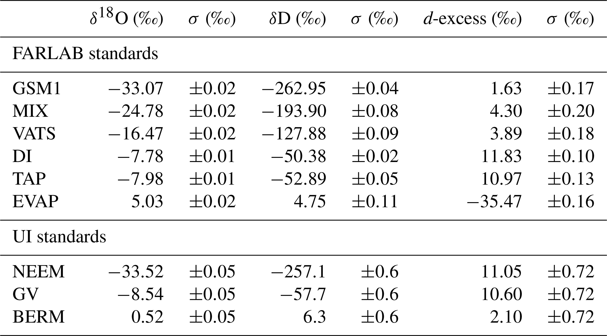
Table 3Summary of the experiment design ordered by the aims and including the dependency on the vapour-generating method, the dependency on the tested instrument, the long-term stability of the dependency behaviour, the influence from the dry gas supply, and the influence of the measuring sequence.
2.3 Standard waters
To identify the influence of the isotope composition on the mixing ratio dependency, we have used multiple internal standard waters calibrated on the international VSMOW2–SLAP2 scale to characterise the mixing ratio dependency. The standard waters include four laboratory standards in use at the Facility for Advanced Isotopic Research and Monitoring of Weather, Climate and Biogeochemical Cycling (FARLAB) of the University of Bergen and three laboratory standards in use at the isotope laboratory of the University of Iceland (UI; Table 2). For the FARLAB standards, one is obtained from snow in Greenland (GSM1), one is mountain snow from Norway (VATS), one consists of deionised tap water at Bergen (DI), and one is evaporated DI water (EVAP). Besides the four laboratory standards, we have also used an even mixing between GSM1 and VATS (MIX) and the uncalibrated deionised tap water (TAP). For the UI standards, one is from snow at the North Greenland Eemian Ice Drilling (NEEM) site in Greenland, one consists of groundwater in Reykjavik (GV), and one is Milli-Q® purified water based on ocean water from Bermuda (BERM). The isotope compositions of all the waters used span from −33.52 ‰ to 5.03 ‰ for δ18O and from −262.95 ‰ to 6.26 ‰ for δD (Table 2).
2.4 Vapour-generation methods
We use two methods to generate vapour for characterising the isotope composition–mixing ratio dependency of the three instruments, namely discrete liquid injections and continuous vapour streaming. These are essentially two ways of generating a vapour sample to be analysed by the infrared spectrometers. Both methods involve the injection of a liquid standard water into a heated evaporation chamber in which the injected water is completely evaporated and mixed with a dry matrix gas.
2.4.1 Dry gas supply
Previous studies of Picarro CRDS analysers preceding the L2140-i show that the matrix gas has an influence on the characterisation of the mixing ratio dependence in the CRDS isotope measurement of water vapour (Aemisegger et al., 2012; Johnson and Rella, 2017). It is therefore important to know the influence of the matrix gas on the isotope composition–mixing ratio dependency to determine, depending on the measurement situation, a preferred method for obtaining the final correction relationship. The manufacturer recommends a customer-supplied gas drying unit (e.g. Drierite desiccants) to supply dry gas for the Standard Delivery Module (SDM) unit. Here we either used a single drying unit with ambient air or dry gas cylinders that contain synthetic air (synthetic air 5.5, purity 99.9995 %; Praxair Norge AS) or N2 (Nitrogen 5.0, purity >99.999 %; Praxair Norge AS). We have tested the three types of dry gas supply, with the characterisation on instrument HIDS2254, for continuous vapour streaming, and we have characterised the three analysers using synthetic air and/or N2 for discrete liquid injections. Ambient air dried through Drierite can still contain some moisture (typically about 200 ppmv when the ambient water vapour is around 10 000 ppmv), which can contribute a non-negligible fraction to the measured isotope composition at low mixing ratios (e.g. 10 % below 2000 ppmv). The use of several drying units in a row, which includes the vertical arrangement of drying units to prevent preferential gas flow, and careful handling of tubing tightness may provide the same background mixing ratio as with a gas cylinder (Kurita et al., 2012), but that has not been tested here.
2.4.2 Discrete liquid injections
The discrete liquid injections repeatedly generate vapour pulses by injecting between 0 and 2 µL of standard water from 1.5 mL PTFE/rubber-septum sealed vials with a 10 µL syringe (VWR, part no. 002977). Injections are operated by an autosampler (A0325; Picarro, Inc., USA) or by manual injection. Vaporisation of liquid water is achieved in a Picarro vaporiser (A0211; Picarro, Inc., USA) set to 110 ∘C. The vaporiser mixes the water vapour with synthetic air or N2 from a gas cylinder at a pressure set to ∼170 hPa. The vaporiser chamber seals off for a few seconds to allow for sufficient mixing between the vapour and the matrix gas before delivering the mixture to the analyser at a highly stable mixing ratio.
Before switching to a new standard water, 8–12 injections of the new standard water at a mixing ratio of ∼ 20 000 ppmv were applied each time to account for the memory effects from the previous injections. Then the sequence begins at the lowest (∼500 ppmv) and ends at the highest (∼23 000 ppmv) mixing ratio. Various mixing ratios are obtained by adjusting the injection volume in the 10 µL syringe. The injection volume was modified to be between 0.05 and 2.5 µL with a step of 0.05 µL, resulting in mixing ratios between approximately 500 and 23 000 ppmv with a step of ∼ 450 ppmv. Four injections in the high-precision mode (longer measurement period with approximately 10 min per injection) were applied to each mixing ratio, and the last three injections were then averaged for further analysis. Injections with an injection volume of 2 µL (∼19 000 ppmv) were carried out at the beginning and end of a sequence to account for potential instrument drift. A sequence for one standard water lasts approximately 35 h. The instrument drift within a sequence typically has a magnitude of (0.05±0.02) ‰, (0.7±0.1) ‰, and (0.4±0.1) ‰ for δ18O, δD, and d-excess respectively. The drift is 4–7 times larger than the uncertainty associated with the estimated drift but 1 order smaller than the deviation introduced by the mixing ratio dependency; it is corrected by assuming a temporal linearity during the sequence period.
Manual liquid injections were carried out during a field deployment where no autosampler was available. During manual injections, it is challenging to maintain a constant injection volume, and it is thus difficult to achieve a precise control of the water vapour mixing ratios. In this case, only injection volumes between 0.2 and 1.6 µL with a step of ∼0.2 µL are employed, which roughly corresponds to mixing ratios between 2400 and 24 000 ppmv with a step of ∼3000 ppmv. Despite the shorter measurement period (about 6 h), the instrument drift within a sequence increased by a factor of 2–3 for δ18O ((0.16±0.03) ‰) and δD ((1.65±0.18) ‰), resulting in a drift of (0.37±0.22) ‰ for d-excess. The relatively high instrument drift, when compared to the autosampler injections in the laboratory, is most likely due to the uncertainty introduced by the variable injection volume and the operation on a container on the deck of a research vessel (Renfrew et al., 2019). Instrument drift is corrected by assuming linear drift during each characterisation experiment. In all characterisation experiments, we applied three to five FARLAB standard waters when using an autosampler or three UI standard waters in the case of manual injections.
2.4.3 Continuous vapour streaming
To test the influence of the vapour-generation method, we used the continuous water vapour streaming of two laboratory standard waters (DI and GSM1). A continuous vapour stream is generated via a so-called Standard Delivery Module (SDM, A0101; Picarro, Inc., USA). The SDM is a device with two syringe pumps that provides automated delivery of two standard waters at up to three water concentrations per standard. The standard water is delivered to the Picarro vaporiser where it is instantly vaporised at 140 ∘C and simultaneously mixed with a dry matrix gas. The routines for vapour streaming at the different mixing ratios applied here follow recommendations by the manufacturer to characterise each instrument's mixing ratio dependency (SDM user manual; Picarro, Inc.). Mixing ratios between 600 and 24 000 ppmv were obtained by adjusting the liquid water injection speed of the syringe pumps from 0.002 to 0.8 µL s−1. The generated standard vapour is continuously delivered to and measured by the spectrometer. During the characterisation, we measured about 25 mixing ratios at a step of ∼1000 ppmv (0.003 µL s−1) for each standard water. Each mixing ratio is measured for 20–40 min, and the averaged value of a 5 min period close to the end of the measurement is used in the analysis. Due to unstable calibration performance, only sections of 1–2 min were used for the characterisations done in July 2016 and February 2018 for the laboratory standard DI on instrument HIDS2254.
A measurement sequence of standard GSM1 with ambient air dried through Drierite shows that the magnitude of the instrument drift during a 22 h measurement with the SDM is similar to that of the liquid injection with an autosampler. However, due to the lower precision of the SDM measurement, the instrument drift is comparable to – (0.10±0.09) ‰ and (0.96±0.36) ‰ for δ18O and δD respectively – or smaller for the uncertainty associated with the estimated drift, i.e. (0.24±0.78) ‰ for d-excess. Therefore, except for the measurement with standard GSM1 mentioned previously, the measurements with the SDM are not corrected for instrument drift.
2.5 In situ measurement data for studying the impact of the isotope composition–mixing ratio dependency correction
In order to test the impact of the isotope composition–mixing ratio dependency correction on actual measurements, we applied the proposed correction scheme to two data sets obtained from in situ vapour measurements during the Iceland–Greenland Seas Project (Renfrew et al., 2019) on board a research aircraft (analyser HIDS2254) and a research vessel (analyser HKDS2038) in March 2018 on the Iceland–Greenland seas (∼68∘ N, 12∘ W).
The HIDS2254 analyser was installed on board a Twin Otter research aircraft. The instrument was fixed on a rack on the right side of the non-pressurised cabin. A 3.5 m stainless-steel tube with 3∕8 in. diameter, insulated and heated to 50 ∘C, was led from a backward-facing inlet located behind the right cockpit door to the analyser. A backward-facing inlet was selected to ensure that only vapour (and not particles or droplets) would be sampled. A manifold pump was used to draw the vapour through the inlet at a flow rate of about 8 slpm. The HIDS2254 took a sub-sample through a 0.2 m stainless-steel tubing in low-flow mode at a flow rate of ∼35 sccm. The selected vapour measurements from the aircraft were taken in the lower troposphere above the Iceland Sea during a cold air outbreak (CAO) on 4 March 2018. The particular water vapour measurement segment utilised here was taken during a 9 min long descent of the aircraft from 2900 to 180 m a.s.l. A Greenland blocking associated with northerlies in the Iceland–Greenland seas caused cold atmospheric temperatures, with an average of −12 ∘C at altitudes below 200 m. Accordingly, mixing ratios at low levels ranged from 2000 to 2700 ppmv. At higher levels, mixing ratios were as low as about 900 ppmv. After applying any correction schemes (see below), the water vapour isotope data from the aircraft are calibrated to the VSMOW2–SLAP2 scale using the long-term average of calibrations, with internal FARLAB laboratory standards on GSM1 and DI, by using the SDM from before and after the flight survey (details described in a forthcoming publication).
For the vapour measurements on board the research vessel (R/V Alliance), the HKDS2038 analyser was installed inside a heated measurement container that was placed on the crew deck at about 6 m above the water's surface. The ambient air was drawn into the container with a flow rate of around 8 slpm by a manifold pump through a 5 m long 1∕4 in. stainless-steel tube and was heated to about 50 ∘C with self-regulating heating tape. The tube inlet was mounted 4 m above the deck and was protected from precipitation with a downward-facing tin can. The selected time period from the research vessel was acquired during a CAO event between 14 and 16 March 2018. At the beginning of the event, the mixing ratio dropped from 6000 to below 3000 ppmv within 2 h and then stayed at around 3000 ppmv for about 24 h before it increased to 8000 ppmv again.
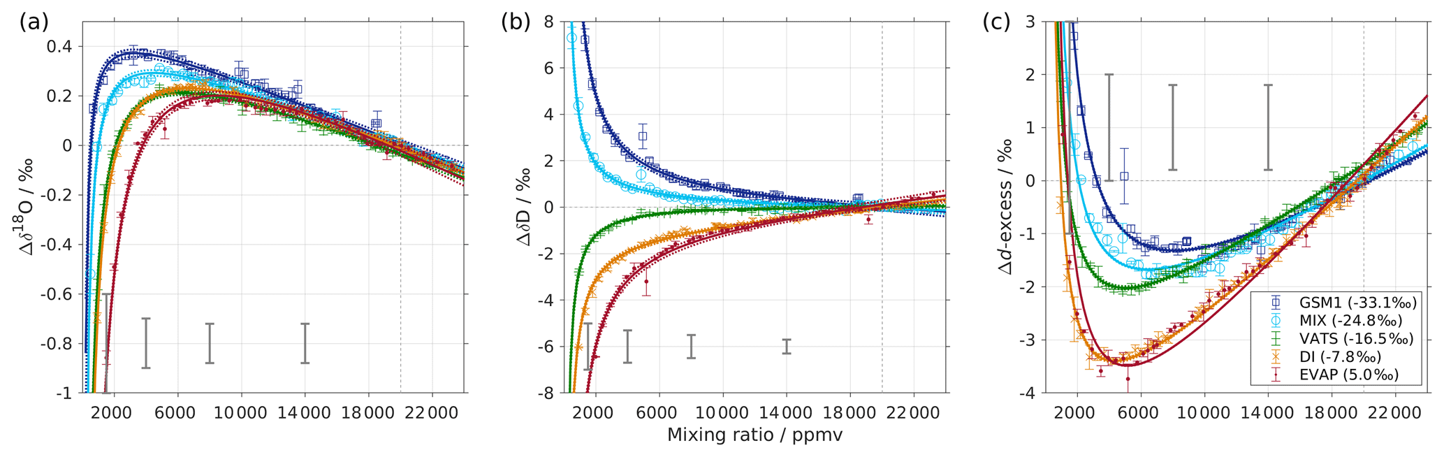
Figure 1Mixing ratio dependency of uncalibrated measurements for (a) δ18O, (b) δD, and (c) d-excess for five standard waters (GSM1, MIX, VATS, DI, and EVAP) on instrument HIDS2254 (Picarro L2130-i) with discrete liquid injections via an autosampler (experiment 1). Mixing ratio dependency is expressed as the deviation Δ of the measured isotope composition at each mixing ratio with respect to the reference mixing ratio of 20 000 ppmv. The symbol and error bar represents the mean and the standard deviation of the mean for the last three of a total of four injections at each mixing ratio. Solid lines are fits with the function . Dashed lines are the 95 % confidence interval for the corresponding fit. Measurements and fits for d-excess are calculated with . The typical 1 standard deviation of a single injection at the corresponding mixing ratio is indicated with grey error bars. Two outliers (at about 4300 and 8900 ppmv) are removed from the GSM1 measurements, and one outlier (at about 9000 ppmv) is removed from the VATS measurements.
In this section we present the isotope composition–mixing ratio dependency from the characterisation result for the HIDS2254 instrument (Fig. 1). The characterisation is carried out using the method of discrete liquid injections (experiment 1). At each mixing ratio, a total of four injections are carried out in high-precision mode, and the last three injections are averaged for further analysis. The uncertainty at each mixing ratio is calculated as the standard deviation of the three injections taken; this standard deviation (colour error bars in Fig. 1) is substantially smaller than the standard deviation of one single injection (indicated by thick grey error bars in Fig. 1).
The mixing ratio dependency for δ18O, displayed as the deviation Δδ18O, exhibits a skewed, inverse-U shape (Fig. 1a) for all of the water standards. As an example, standard GSM1 (dark blue symbols) starts with a deviation of −0.1 ‰ for a high mixing ratio of 23 000 ppmv, becomes positive after passing 20 000 ppmv, and continues increasing until reaching a maximum of around 3000 ppmv. Then Δδ18O quickly drops at lower mixing ratios and becomes negative again at around 500 ppmv. As the mixing ratio decreases further, the magnitude of the deviation increases substantially. Notably, the mixing ratio dependencies of the other four standard waters (light blue, green, orange, and red symbols for MIX, VATS, DI, and EVAP respectively) also depict an inverse-U shape. However, the maxima become smaller and shift towards higher mixing ratios (bottom right in Fig. 1a) with a more enriched isotope composition. This isotope-composition-related shift leads to an enlarged difference of Δδ18O between any of the standard waters. For example, Δδ18O for GSM1 (dark blue symbols) and EVAP (red symbols) differ by ∼0.9 ‰ at 2000 ppmv and by 2.0 ‰ at 1000 ppmv.
The isotope-composition-related shift is even more pronounced for ΔδD (Fig. 1b). For the standard waters with relatively depleted isotope compositions (GSM1 – dark blue; and MIX – light blue), ΔδD is positive and becomes larger as the mixing ratios decrease. For the standard waters with relatively enriched isotope compositions (VATS – green; DI – orange; and EVAP – dark red), ΔδD becomes more negative with decreasing mixing ratios. This leads to an increasing divergence of the mixing ratio dependency at ∼15 000 ppmv and below. For example, ΔδD for GSM1 (dark blue) and EVAP (red) differ by ∼11 ‰ at 2000 ppmv and by ∼21 ‰ at 1000 ppmv.
The isotope composition dependency of Δδ18O and ΔδD has a substantial impact on the mixing ratio dependency of Δd-excess for different water standards. The mixing ratio dependency of Δd-excess below ∼15 000 ppmv now exhibits a U-shape, with the minimum located between 4000 (DI – orange) and 7000 ppmv (GSM1 – dark blue). The deviation for GSM1 (dark blue) and EVAP (red) differs by ∼3.8 ‰ at 2000 ppmv and by ∼5.3 ‰ at 1000 ppmv.
In summary, this characterisation shows that the mixing ratio dependency varies systematically according to the isotope composition of the measured standard water. It is most pronounced at low mixing ratios (below 10 000 ppmv) and also increases at lower mixing ratios. The substantial deviations are clearly important for in situ water vapour measurements in dry environments, particularly when the water vapour has large variations in the isotope composition. As demonstrated in Sect. 4, we find that this systematic isotope composition–mixing ratio dependency occurs irrespective of the vapour-generation method and dry gas supply and exists in a similar form in all three of the CRDS spectrometers characterised here.
The mixing ratio dependency of HIDS2254 seems to vary systematically with the isotope composition of the water standards, suggesting a potential spectroscopic origin (Sect. 7). This isotope composition–mixing ratio dependency will not be sufficiently removed by a uniform correction based on a single water standard. However, the dependency can be corrected if we can establish a correction function that takes both the mixing ratio and the isotope composition into account. First we investigate how robust and stable the described isotope dependency is over time before proposing a correction framework based on our characterisation results.
We carefully analysed the robustness of the isotope composition–mixing ratio dependency with respect to the choice of the method for vapour generation, the dry gas supply, the measuring sequence, individual instruments and instrument type, and its stability over time using 15 experiments in total (Table 1). Here we provide a summary of the results from these different experiments, with the detailed results given in Appendix A.
The robustness test indicates that the isotope composition–mixing ratio dependency is consistent across the two tested vapour-generation methods, i.e. discrete liquid injections and continuous vapour streaming (Appendix A1; Fig. A1a–c). Characterisations with synthetic air and N2 are in agreement for δD but deviate for δ18O (Appendix A2; Fig. A1d–f). A particularly substantial disagreement is found for the experiment using Drierite. This is likely caused by the contribution from water vapour remaining in the matrix air after the drying unit. The measuring sequence from high to low mixing ratios, or the reverse, shows a great similarity in the results, indicating that the potential hysteresis effects are not substantial (Appendix A3; Fig. A1g–i). However, we do note a different result for δ18O at the lowest mixing ratio during one of the repeated experiments with MIX water (not shown). We suspect that the high sensitivity of the isotope composition–mixing ratio dependency at this range of δ18O values could lead to pronounced deviations. While this aspect deserves further attention, we consider it as being second order with regards to the existence and cause of an isotope composition–mixing ratio dependency in the investigated CRDS instruments. Tests of all three analysers with discrete autosampler injections and N2 as the matrix gas show a similar isotope composition–mixing ratio dependency in all three analysers investigated (Appendix A4; Fig. A2). The repeated characterisation of analysers HIDS2254 and HKDS2038 during a time period of up to 2 years shows that the isotope composition–mixing ratio dependency is an instrument characteristic that is, at the first order, constant over time (Appendix A5, Fig. A3).
In summary, the isotope composition–mixing ratio dependency is, at the first order, robust across a range of key parameters and stable over time. However, it is also apparent that individual instruments have a different strength, and it is the shape of the instrument characteristic that requires individual correction. In the next sections, we apply and evaluate a new scheme to correct for the isotope composition–mixing ratio dependency.
We now use the characterisation result previously obtained from instrument HIDS2254 as an example of how to derive a correction procedure for the isotope composition–mixing ratio dependency by following six sequential steps. Due to the systematic behaviour observed in Fig. 1, we chose a simple, traceable fitting procedure to obtain the two-dimensional correction function that can potentially be related to a physical cause. For the sake of simplicity, the equations in the following paragraphs are formulated to be valid for both δ18O and δD.
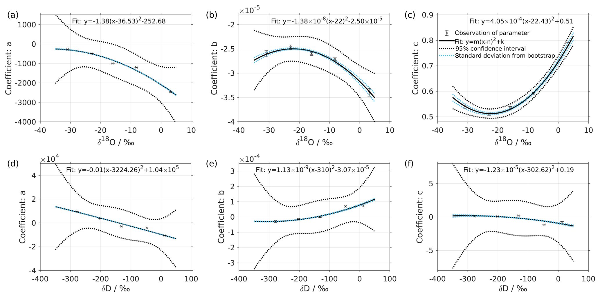
Figure 2Dependency of fitting coefficients a, b, and c on δ18O (a–c) and on δD (d–f). The coefficients a, b, and c are from the fits for the five standard waters in Fig. 1. The solid line is the quadratic fit, with . The black dotted line shows the 95 % confidence interval. The blue dotted line shows the standard deviation estimated from a bootstrapping method.
5.1 General formulation
-
We obtain the mixing ratio dependency for each water standard as raw (uncorrected, uncalibrated) measurements of the isotope compositions. The water standards thereby cover a wide range of isotope compositions and different mixing ratios, particularly also at low mixing ratios.
-
We express the mixing ratio dependency for each water standard as the deviation of the raw measurements to the reference value at 20 000 ppmv (Eq. 3). The reference value is obtained from a linear interpolation between the closest measurements above and below 20 000 ppmv. These deviations are denoted as Δδ18O, ΔδD, and Δd-excess as described in Sect. 2.1.
-
A suitable fitting function is fitted to the mixing ratio dependency of each standard water. Here we used fitting functions with the following form:
where x is the mixing ratio, δ indicates the isotope composition of the standard waters, and aδ, bδ, and cδ are fitting coefficients for each water standard and isotope species.
-
We express the obtained fitting coefficients as a function of the isotope composition as a(δ), b(δ), and c(δ) for all the standard waters (Fig. 2, symbols). This reveals a dependency of the fitting coefficients on the isotope composition of the water standard. We now fit a suitable function to this dependency by using the following quadratic polynomial:
where δ is the isotope composition and m, n, and k are the respective fitting coefficients of the quadratic polynomials.
-
By replacing the parameters aδ, bδ, and cδ in Eq. (4) with their parametric expressions in Eq. (5), we obtain the generalised fitting for the mixing ratio dependency, which is a function of both the mixing ratio x and the isotope composition of the measured water δ as follows:
-
Using Eq. (6), we can now correct the measured isotope compositions to a reference mixing ratio at 20 000 ppmv when given any measured raw mixing ratio and isotope composition within the range investigated here. Thus, the isotope composition at 20 000 ppmv (δcor) is the unknown; its analytical solution is found by solving the following equation:
where h is the measured raw mixing ratio and δmeas is the measured isotope composition at that mixing ratio. The right-hand side of the equation is the isotopic deviation determined from Eq. (6). The coefficients a(δcor), b(δcor), and c(δcor) are determined from Eq. (5). Equation (7) is a quadratic function; the procedure to obtain its analytical solution is given in Appendix C.
5.2 Correction function for analyser HIDS2254
We now exemplify the general steps given previously for the HIDS2254 analyser. The results from step 1 and 2 for HIDS2254 are presented in Sect. 3. Here we use a range from −33.07 ‰ to 5.03 ‰ for δ18O and from −262.95 ‰ to 4.75 ‰ for δD, with mixing ratios between 500 and 25 000 ppmv (experiment 1 in Table 1).
Table 4Fitting coefficients for the mixing ratio dependency behaviour of the five standard waters measured with HIDS2254. Coefficients a, b, and c are calculated with respect to the fitting function . The reported uncertainty is 1 standard deviation. The fitting lines are shown in Fig. 1.
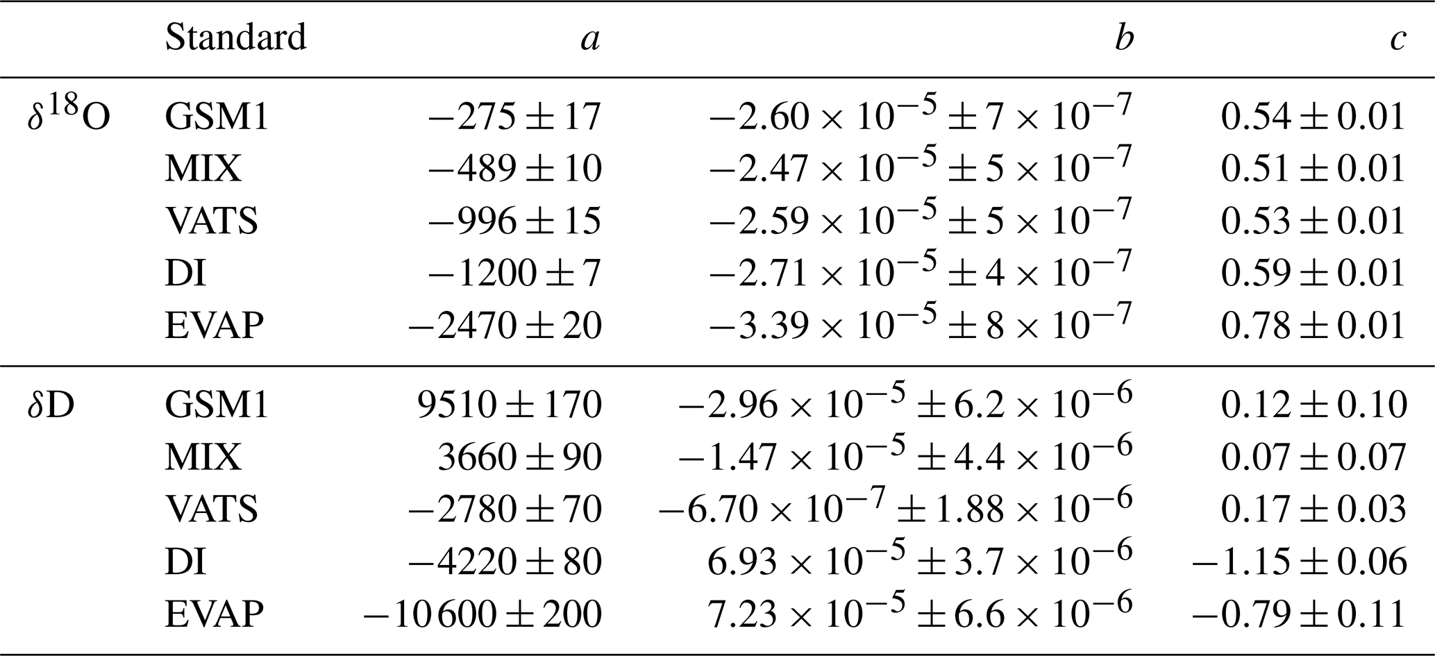
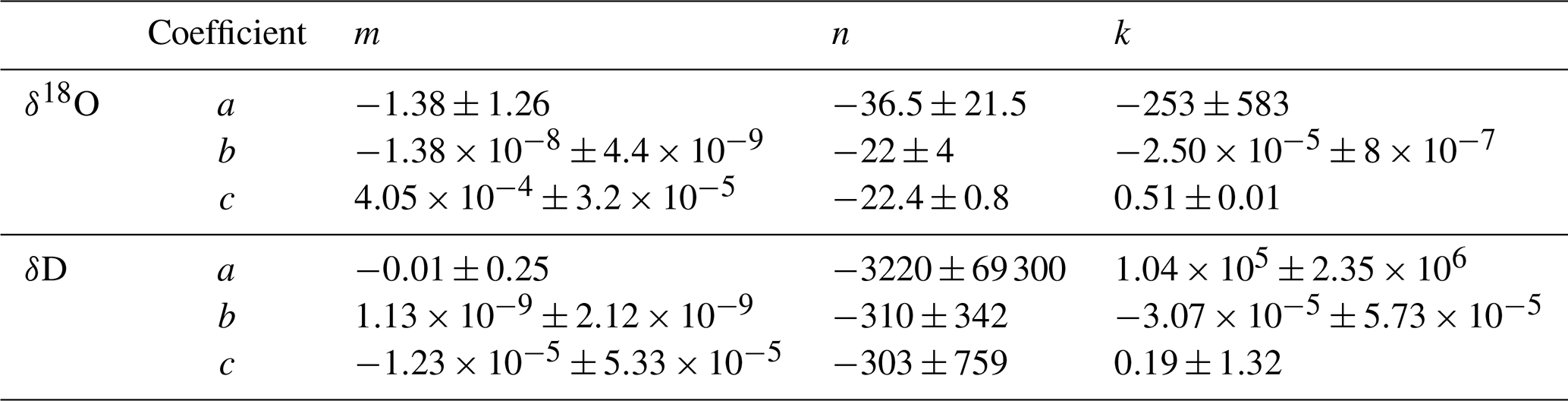
Table 5Fitting coefficients for the isotope composition dependency of the mixing ratio dependency coefficients a,b, and c in Table 4. Coefficients m,n, and k are with respect to the fitting function . The reported uncertainty is 1 standard deviation. The fitting lines are shown in Fig. 2.
The coefficients aδ, bδ, and cδ obtained in step 3 from Eq. (4) for the five standard waters measured on instrument HIDS2254 are given in Table 4. While the magnitude differs between the coefficients, scaling analysis shows that each of the terms (, bx, and c) on the right-hand side of Eq. (4) contributes similarly to the isotope composition–mixing ratio dependency (not shown). The fitting results from step 4 are shown in Fig. 1 (solid colour line). The choice of this type of function captures the behaviour of the isotope composition–mixing ratio dependency for both Δδ18O and ΔδD of each standard water. Thus, the fit for Δd-excess is calculated from the fit of Δδ by .
The coefficients m, n, and k obtained in step 4 in Eq. (5) are given in Table 5. The fitting results (solid line) with the fitting uncertainty (95 % confidence interval; black dotted line) are shown in Fig. 2. Since we only fit 5 data points, the fitting uncertainty is large, which results in a relatively large standard deviation for the isotope composition deviations Δδ. This large standard deviation for Δδ can be reduced by using a bootstrapping approach (Efron, 1979) to estimate the fitting uncertainty in Eq. (5; Appendix B).
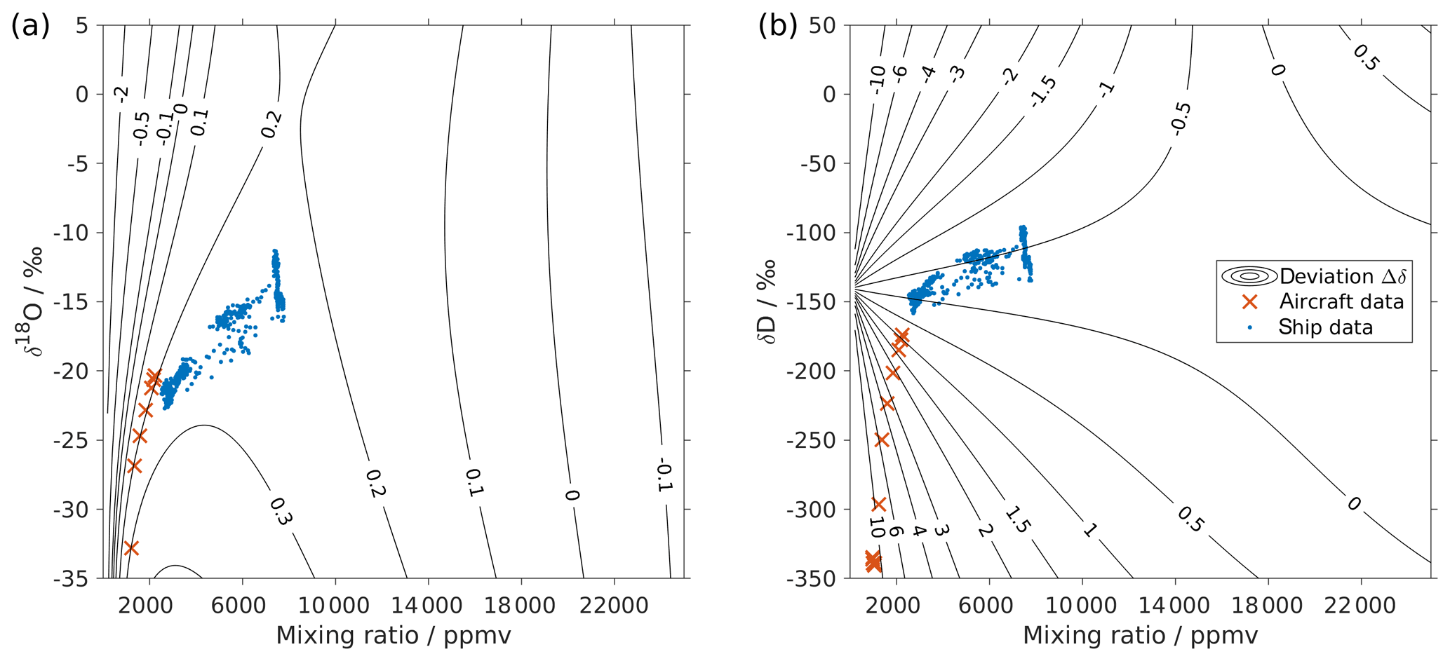
Figure 3Surface function of the isotopic deviations for (a) δ18O and (b) δD based on the isotope composition–mixing ratio dependency of instrument HIDS2254 (Picarro L2130-i). The x axis is the raw mixing ratio, and the y axis shows the raw isotope composition at 20 000 ppmv. Contours with numbers indicate the isotopic deviation of Δδ. Symbols show the isotope measurements over the Iceland Sea: measurements averaged to 1 min from an aircraft in the lower troposphere (red crosses) and measurements at a 10 min resolution from a research vessel (blue dots). The measurements from the aircraft were done with instrument HIDS2254 (Picarro L2130-i), and measurements on the research vessel were done with instrument HKDS2038 (Picarro L2140-i).
Following step 5, this results in a two-dimensional correction surface for each isotopologue as shown in Fig. 3 (black contours). For illustration purposes, some contours below 4000 ppmv are omitted for both δ18O and δD. The isotope composition–mixing ratio dependency for both δ18O and δD increases substantially at low mixing ratios. For δ18O, the deviation changes from positive to negative as the mixing ratio decreases below ∼4000 ppmv. For δD, the deviation increases below 10 000 ppmv and splits into both positive and negative contributions – depending on the isotope composition. The uncertainty (1 standard deviation) for the deviation Δδ is typically 1 order of magnitude smaller than the Δδ values at the corresponding position.
The surface function exhibits the same features as those determined by the experimental results, underlining that the fitting procedure reflects the main characteristics of the isotope composition–mixing ratio dependency from the experimental data. At 20 000 ppmv, the correction function is not exactly 0, as the fit that is based on all the measurements is not constrained to the point [20 000, 0] ppmv. This deficiency could be addressed by a modified fitting procedure. Below 500 ppmv, the correction function has larger uncertainties due to the lack of measurements at this mixing ratio range. Note that the fitting functions used in Eqs. (4) and (5) are purely phenomenological and do not result from a particular physical model. Still, we recommend the proposed parameterisation to characterise individual instruments.
We now investigate the impact of the isotope composition–mixing ratio dependency correction in situ measurements of the isotope composition of water vapour with two CRDS analysers installed on board a research aircraft (HIDS2254) and a research vessel (HKDS2038; see Sect. 2.5).
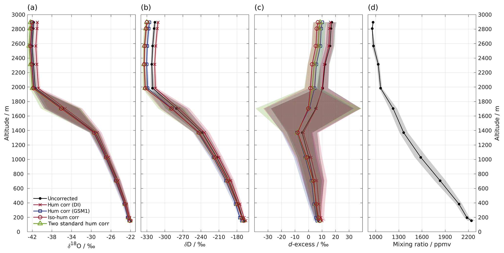
Figure 4Vertical profiles of (a) δ18O, (b) δD, (c) d-excess, and (d) mixing ratio measured by instrument HIDS2254 on an aircraft above the Iceland Sea on 4 March 2018. Shown are 1 min averaged profiles of the uncorrected data set (black line with dot) and four data sets using different isotope composition–mixing ratio dependency correction schemes as follows: the mixing ratio dependency of standard DI (orange curve with cross); standard GSM1 (blue curve with square); the isotope composition–mixing ratio dependency surface function (red curve with circle); and two mixing-ratio-dependency-corrected standards (green curve with triangle). All of the data sets are calibrated according to the VSMOW2–SLAP2 scale. Shading shows the total uncertainty (1 standard deviation) for the corresponding profiles. Note that the profile of δD has been adjusted 30 s forward to account for the longer response time of molecular HD16O. The large uncertainty between 1400 and 2000 m for d-excess is partly due to the rapid evolution of the δ18O and δD profiles, and it is partly due to the dephasing between the δ18O and δD profiles caused by different response times.
6.1 Impact on the aircraft measurements
Low water vapour mixing ratios and a relatively wide range of (depleted) isotope compositions make water vapour isotope measurements from a research aircraft particularly suitable for demonstrating the impact of the new isotope composition–mixing ratio dependency correction. Figure 4 shows a vertical profile of 1 min averaged water vapour isotope measurements above the Iceland Sea (Sect. 2.5). During the descent of the aircraft from 2900 m a.s.l. to the minimum safe altitude, the water vapour mixing ratio gradually increases from about 800 ppmv at the top to 2300 ppmv near the surface (Fig. 4d). The stable isotope profiles (Fig. 4a–c) show three main characteristics. Above about 2000 m a.s.l., δ18O and δD are depleted ( ‰ and −320 ‰) with d-excess between 10 ‰ and 20 ‰. Between 2000 and 1400 m a.s.l., there is a transition where δ18O and δD increase to around −30 ‰ and −240 ‰, respectively, and d-excess decreases to ‰. Below 1400 m a.s.l., δ18O, δD, and d-excess gradually increase until reaching about −22 ‰, −170 ‰, and 8 ‰, respectively, near the surface. The uncertainty (1 standard deviation) of the profile is obtained using the uncertainty propagation law, including the uncertainty (1 standard deviation) of the 1 min averaged data set (here the dominating source of uncertainty) and the uncertainty of the correction scheme.
First we investigate the impact of the new correction scheme introduced here. This correction, abbreviated as iso-hum-corr, modifies the uncorrected data set in the region above 2000 m a.s.l. by about −0.4 ‰ and −13.3 ‰ for δ18O and δD, respectively, resulting in a change of about −10.4 ‰ for d-excess (Fig. 4; red circles vs. black dots). The impact of applying the new correction scheme to the aircraft measurements can be understood by examining where the data sets align in the correction surface function (Fig. 3; red crosses). For both δ18O and δD, the aircraft data set is characterised by a low mixing ratio and depleted isotope compositions, and it is clustered in the bottom-left corner of the surface function. This is the most sensitive area of the correction, thus causing the largest deviations in the surface function.
To assess the benefit of the new isotope composition–mixing ratio dependency correction, we take this new correction scheme as the reference scheme and compare its impact to three other correction schemes. The first scheme only corrects for the mixing ratio dependency based on standard DI (hum-corr-DI, Fig. 4; orange crosses). The second correction follows the same procedure but is based on standard GSM1 (hum-corr-GSM1, Fig. 4; blue squares), and the third correction follows an approach proposed by Bonne et al. (2014) for in situ vapour measurements in southern Greenland. Instead of correcting the mixing ratio dependency for the vapour measurements, the Bonne et al. (2014) approach corrects the mixing ratio dependency for the calibration standards. Thus, by assuming that the mixing ratio dependencies of the two employed standards remain stable during the measurement period, the measured isotope compositions of these two standards are corrected by using the mixing ratio dependency function to the ambient air mixing ratio of each single vapour measurement. Then, the linear regression computed from these two corrected standard measurements against their certified values is applied to calibrate the vapour measurement to the VSMOW2–SLAP2 scale. This scheme is hereafter referred to as 2-std-hum-corr (Fig. 4; green triangles).
The different correction schemes modify the uncorrected data set differently. The δ18O profile is only marginally affected by the correction below 1400 m a.s.l. (Fig. 4a). For the measurements above 1400 m a.s.l., differences become more pronounced but are masked by the large uncertainty as the aircraft was descending through a strong mixing-ratio gradient. All corrections show clear deviations at elevations above 2000 m a.s.l., and we focus our comparison on this region. The hum-corr-DI stands out, with a positive correction of about 0.8 ‰, while the other three schemes induce a negative correction of between −0.3 ‰ and −0.7 ‰. The δD profile exhibits a similar pattern but with more apparent differences between the correction schemes (Fig. 4b). This results in an even more pronounced correction in the d-excess profile (Fig. 4c).
The impact of applying the correction scheme using single standard water (thus accounting for only mixing ratio dependency) relies on the choice of the used standard water. Using the hum-corr-DI correction introduces the largest deviation (1.1 ‰, 18.3 ‰, and 9.5 ‰ for δ18O, δD, and d-excess respectively), while using the hum-corr-GSM1 correction produces results much closer to that of the reference scheme (with an offset of 0.1 ‰ and 4.2 ‰ for δ18O and δD, respectively, and 3.4 ‰ for d-excess). For this specific aircraft measurement (where the surface condition is already quite dry during the cold air outbreak event) the isotope composition of standard GSM1 happens to closely resemble the average isotope composition of the measurement. However, in the case of a previously unknown range of isotope compositions or strongly varying conditions, a comprehensive characterisation of mixing ratio dependency with multiple standard waters can provide advantages and should be preferred. Unknown ranges are particularly likely for atmospheric measurements of vertical profiles in humid regions (e.g. the tropics and subtropics) or over a wide area from moving platforms.
Finally, applying the alternative calibration approach (2-std-hum-corr) used in Bonne et al. (2014) results in only slightly more depleted isotope values than the reference, with an offset of about −0.3 ‰ and −0.5 ‰ for δ18O and δD, respectively, resulting in a change of 1.7 ‰ for d-excess. The small discrepancy between the 2-std-hum-corr and iso-hum-corr is mainly due to three factors. First, depending on the number of the used standard waters, the interpolation scheme for the isotopic deviations in between those of the used standard waters can be different. The 2-std-hum-corr makes use of the mixing ratio dependency functions of only two standard waters. In this way, the deviations can only be linearly interpolated between the two standard waters. In contrast, the reference scheme is able to account for non-linearities during interpolation by measuring five standard waters. Second, 2-std-hum-corr corrects the two standard waters to the mixing ratio of the measurement while the reference scheme corrects the measurement to the mixing ratio of the two standard waters (i.e. the reference mixing ratio). Based on the mixing ratio dependency feature of the two standard waters, the choice of correcting the two standard waters will result in a higher slope for the VSMOW2–SLAP2 calibration line. Consequently, the measurements after calibration are stretched to two ends, i.e. the measurements with the isotope composition close to that of standard DI become more enriched and those close to that of standard GSM1 become more depleted. Finally, the mixing ratio dependency functions for GSM1 and DI in 2-std-hum-corr (using the individual fit for GSM1 or DI respectively) are not exactly identical to those used in the reference scheme (from the surface function determined by the measurements of five standard waters). Despite the small discrepancy, the consistent results of 2-std-hum-corr with that of the reference scheme indicate that a correction scheme using the mixing ratio dependency functions of only two standard waters covering the measured isotope composition range can work sufficiently well in certain situations.
6.2 Impact on the ship-based measurements
Applying the four different correction schemes to the ship-based measurement data has a much weaker impact on the corrected series of vapour measurements (not shown). After applying our isotope composition–mixing ratio dependency correction scheme, the uncorrected data set changes to the order of 0.06 ‰ and 0.15 ‰ for δ18O and δD, respectively, leading to a change to the order of −0.5 ‰ for d-excess. This is mainly because these ship measurements were carried out at the ocean surface, with relatively high mixing ratios (from 2500 to 8000 ppmv) and less-depleted isotope compositions (−23 ‰ to −12 ‰ for δ18O and −160 ‰ to −100 ‰ for δD) compared to the aircraft measurements. As shown in Fig. 3, the ship data (blue dots) are coincidentally located in an area with low sensitivity at the correction surface. A linear interpolation between two standards may not capture such a saddle point correctly. This indicates that measurements are not sensitive to the correction of the isotope composition–mixing ratio dependency under all conditions. Ultimately, however, the certainty about a reliable correction will only be achieved with a complete characterisation of the isotope composition and mixing ratios covered by the measurements.
Our careful characterisation experiments show that the isotope composition–mixing ratio dependency affects measurements at low mixing ratios for all three investigated stable water isotope CRDS analysers. Here we discuss possible causes of the isotope composition–mixing ratio dependency. In particular, we explore to what extent this dependency is an artefact from mixing with water remaining within the analyser or whether it is an instrument behaviour resulting from spectroscopic effects.
7.1 Artefact from mixing
If we assume the dependency is as a result of mixing with remnant water, then there would mainly be two candidates for the background moisture source: (1) the remaining water vapour in the dry gas supply and (2) the remaining water vapour from previous measurements in the analyser. By changing the dry gas supply from the ambient air dried through Drierite to synthetic air or N2 from cylinder, which typically provides a dry gas with a mixing ratio below 10 ppmv, we can exclude the possible influence of the background moisture in the dry gas supply. In order to quantify the amount and the isotope compositions of the remaining water vapour from previous measurements, we have applied several successive, so-called empty injections via the autosampler. Thus, no liquid is injected and only dry gas is flushed into the vaporiser. Results from these empty injections show that the remaining water vapour in the system typically has a mixing ratio of about 60–80 ppmv, with its isotope composition closely following those of the previous injections. If the mixing ratio dependency was a result of the mixing between the injected water and the remaining water vapour from previous measurement, then we would expect a mixing of two water vapour masses of the same isotope compositions at different mixing ratios when injecting the same standard water during a characterisation run. As a consequence, we would expect the mixed vapour to have the same isotope composition, which is not the case. Finally, the shape of the isotope composition–mixing ratio dependency with a maximum between 2000 and 6000 ppmv (Fig. 1a) is not consistent with the expectation of a memory effect that would monotonously increase with the decreasing mixing ratio. The slight hysteresis observed during the upward/downward calibration runs indicates that there may be contributions from remnant water on walls or filter surfaces in the analyser, for example, that only exchange once a sufficiently humid air mass is introduced into the analyser. Such contributions do, however, appear to be of second order when compared to the substantial changes of the mixing ratio dependency with the isotope composition.
7.2 Spectroscopic effect
Now we explore the second hypothesis, namely that the isotope composition–mixing ratio dependency is an instrument behaviour resulting from spectroscopic effects. The manufacturer recommends a procedure for water vapour dependency calibration using their SDM, or similar, device (Picarro Inc., 2017), which is similar to what we have employed. While the first-order effect can be removed from a linear fit, there are second-order, non-linear components that become more apparent the more the water concentration changes from the recommended range of operation (5000–25 000 ppmv). In the following paragraphs, we discuss the potential reasons for the origin of the water vapour and isotope dependency from a spectroscopic standpoint that is based on the published literature (Steig et al., 2014; Rella et al., 2015; Johnson and Rella, 2017).
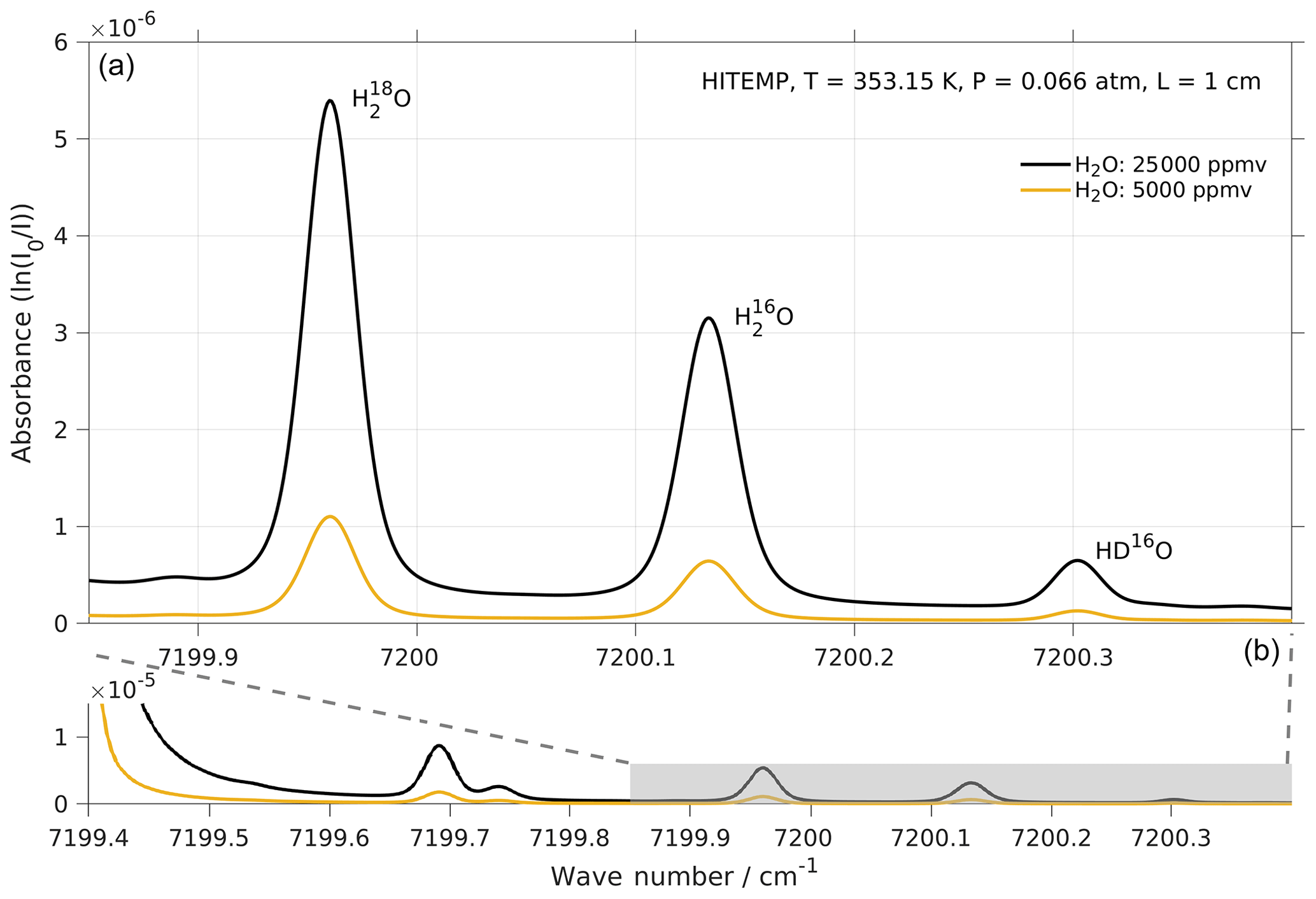
Figure 5Absorption spectrum of , , and HD16O in the frequency range targeted by the laser of Picarro models L2130-i and L2140-i. Simulations with two water concentrations, i.e. 25 000 (black line) and 5000 ppmv (orange line), were performed by using http://spectraplot.com (last access: 19 February 2020) with the HITRAN–HITEMP database (Goldenstein et al., 2017). Simulation parameters are set according to the cavity conditions of the Picarro analyser as follows: T=80 ∘C, P=50 Torr, and L=1 cm. Panel (a) is an enlarged version of the shaded area in panel (b).
The two modules of the CRDS analyser used in our experiments (i.e. Picarro L2140-i and L2140-i) target three absorption lines of water vapour in the region 7199–7200 cm−1, namely near 7199.960, 7200.135, and 7200.305 cm−1 for , , and HD16O respectively (Fig. 5). These absorption lines broaden or narrow, depending on the partial pressure of the gas mixture in the cavity, and can be affected by changes in their baseline due to other strong absorption lines nearby. A fitting algorithm then fits the measured absorption spectrum to an expected model spectrum and adjusts the model parameters in order to minimise the residual error. Broadening/narrowing of lines due to changing gas mixture and baseline shifts are particular challenges to the fitting algorithm (Johnson and Rella, 2017) because this causes residuals that induce instrument error during the fitting procedure.
The L2130-i and earlier spectrometers use the absorption peak as a free parameter in the fitting algorithm. The peak shape and, thus, the peak amplitude can suffer from the above-mentioned broadening/narrowing effect, which introduces potential error under conditions of varying concentration or matrix gases. The fitting algorithms of the L2140-i spectrometers, in contrast, have a higher number of ring downs due to a different strategy for obtaining laser resonance and use a different laser stabilisation scheme. This allows us to fit the integrated absorption, rather than the peak amplitude, of each absorption line. Since the integrated absorption is a constant independent of pressure, the fitting is expected to be more accurate, with a low sensitivity to broadening/narrowing effects arising from changes of water concentrations and background gas compositions (Steig et al., 2014). One part of the retrieval algorithm is the removal of the baseline from the spectrum. To this end, changes in the baseline from nearby strong absorption lines as a result of concentration changes or cross-interference from other gas species is a possible source of error for either fitting algorithm. Other possible sources of error can be absorption loss non-linearities due to small imperfections in the instrument, such as the non-zero shut-off time of the laser and the response time of the ring-down detector (Rella et al., 2015). Unless fitting algorithms take the actual line shapes into consideration directly, some residual effects are likely to persist.
The retrieval of H2O concentration and the stable isotope compositions of δ and δHD16O (identical to δ18O and δD) are implemented in a manner that is similar to the procedure described for CH4 and δ13CH4 (Rella et al., 2015). Considering a linear dependency of absorption to concentration (which is not always true), where the mole fraction of (c18) is related to the absorption peak height α18 with a proportionality constant k18 and an error offset ϵ18, we have the following equation:
Note that the expressions above should apply to both the L2130-i and L2140-i spectrometers, with the only difference being that the absorption peak height is replaced by the integrated absorption (Steig et al., 2014).
Based on the molecular definition of a δ value with respect to the VSMOW2, an isotope ratio of the sample , and of VSMOW2 (Baertschi, 1976), we have the following equation:
The retrieval can then be formulated as follows:
For an ideal spectrometer, the calibration coefficients are constants (i.e. k18=κ18 and k16=κ16), and the calibration offsets are 0 (i.e. ). These assumptions lead to the expected retrieval for a spectrometer as follows:
The actual spectrometer is not ideal, but in most situations it has a highly linear and stable performance (Rella et al., 2015). Nevertheless, it can be calibrated based on the linear dependency of to by using a linear expression with the following form:
where the calibration constants A and B can be determined based on the measurable quantities and the from a reference instrument in the factory. These determined calibration constants deviate slightly from the expected values in Eq. (11). They are then transferred from the reference instrument to each new instrument of the same type (Rella et al., 2015).
If Eq. (12) is used for calibration of the water analysers (not reported in the published literature), then there are two potential sources of error. First, the dependencies on the isotope ratio may not be entirely linear (even when assuming a linear relationship the coefficient is not necessarily a constant and the offset is not necessarily 0) and remain as residuals. Second, the change of this relationship with the differing mixing ratio may remain unexplored. Furthermore, manufacturing tolerances will induce deviations from the reference instrument on which such an initial calibration has been carried out, and instruments therefore have to be calibrated individually to obtain suitable post-processing methods. The initial instrument calibration procedure may therefore be one potential origin for the isotope composition–mixing ratio dependency identified here.
Deviations from an ideal spectrometer stem from the potential spectrometer errors due to small imperfections of the instrument. One possible error is the absorption-loss offset that could occur when the baseline loss is not reproduced well by the fitting algorithm. This absorption offset then leads to a mole-fraction offset, namely ϵ18 in Eq. (8). The measured , including the effect of absorption offset, can be formulated explicitly by following Rella et al. (2015) – and their Appendix S1.1 – as follows:
where α0 is the net absorption loss parameter that should, to the first order, be independent of water concentration and isotope ratio. Comparing this to Eq. (11) for an ideal spectrometer, the additional term of in Eq. (13) creates an inverse relationship with the water concentration and should be responsible for deviations from the ideal spectrometer that are mostly evident at low mixing ratios.
Another possible spectrometer error is the so-called absorption loss non-linearity, which describes effects due to a shorter or longer ring-down time than expected in the optimal range of operations. These effects can be included as additional terms, again by following Rella et al. (2015) – and their Appendix S1.2 – with a non-linear dependency of α18 on α16 (i.e. ) as follows:
The calibration coefficients are thus assumed constant. The non-linearities from spectral crosstalk between and or imperfections in the baseline removal of the absorption spectrum are present in several terms; such effects require the calibration of each individual instrument to be accounted for. When written in this explicit form, it appears consistent with expectations that a systematic isotope composition–mixing ratio dependency may be detected from careful analyser characterisation. The equation can be further simplified as follows:
The difference between Eq. (15) and Eq. (12) represents the deviation from an ideal spectrometer due to non-linearities from imperfections in the baseline removal and spectral crosstalk between and and can be denoted as follows:
The dependency on water concentration (c16) in Eq. (16) appears consistent with the mixing ratio dependency function (Eq. 7) identified in our systematic investigation of three analysers, supporting the hypothesis of a spectrometric origin for the isotope composition–mixing ratio dependency.
A similar form of mixing ratio correction is applied to the 17O measurements using the L2140-i analyser in the study of Steig et al. (2014), and their Eq. 22, in which the integrated absorption area, instead of the peak amplitude, is used to calculate the absorption loss, and the crosstalk between and is modelled with a bilinear relationship. Steig et al. (2014) note that the introduction of an integrated absorption detection leads to a substantially improved behaviour for the mixing ratio dependency over the peak amplitude detection for δ18O but not for δD, with the reason remaining unclear. It is also worth noting that their instrument has not been evaluated for the low mixing ratio range, which is the focus of this paper. It may be possible that part of the identified isotope composition dependency of the mixing ratio dependency stems from the, thus far, lacking systematic analysis of the low mixing ratio range of the analyser for this effect.
One aspect that is not addressed here, but may be valuable for further consideration in the future, is the availability of analysers with higher flow rates of above 300 sccm, for example, for use in research aircraft (Sodemann et al., 2017). Given recent indications that the flow rate affects the isotope composition–mixing ratio dependency (Thurnherr et al., 2020), forthcoming studies should explore the flow rate as an additional parameter. This requires the availability of suitable methods to generate standard vapour at these higher flow rates.
We have systematically investigated the mixing ratio dependency of water vapour isotope measurements for three commercially available, infrared cavity ring-down spectrometers. We found that the mixing ratio dependency varies with the isotope composition of the measured vapour. We define this behaviour as the isotope composition–mixing ratio dependency. The dependency is robustly identified across three similar analysers, regarding several first-order parameters, and is found to be stable over time. Using the characterisation results of five standard waters from a Picarro L2130-i analyser as an example, we propose a correction scheme for this isotope composition–mixing ratio dependency. Using such a correction scheme, we can correct the isotopic measurements for any measured mixing ratio and isotope composition within the range investigated here.
To demonstrate the impact of the mixing ratio dependency correction, we have compared the proposed correction scheme with other published correction schemes, using in situ measurements from dry environments. The impact on the measurements is found to be most substantial at the low mixing ratios. Applying a correction scheme only accounting for the mixing ratio dependency relies on the choice of the standard water used. For an aircraft data set, using the mixing ratio dependency function based on the standard DI produces a large deviation from our proposed scheme; using the mixing ratio dependency based on standard GSM1 produces results similar to our proposed scheme, since it is closer to the average isotope composition of the aircraft data set. Finally, we have investigated the impact of applying a correction scheme used by Bonne et al. (2014). This approach produces results in good agreement with that of our approach. The small discrepancy is due to the interpolation scheme (linear or non-linear) of the isotopic deviation, the choice of correcting mixing ratio dependency of the standards or that of the vapour measurement, and the small discrepancy in the mixing ratio dependency functions of the two standards. The consistent results indicate that a correction scheme using the mixing ratio dependency functions of only two standards covering the isotope composition could be sufficient if the correction surface can be sufficiently approximated by linear interpolation. Using ship measurements made at higher mixing ratio conditions, we find a weaker impact from the different correction schemes.
Given the non-monotonous characteristics of the isotope composition–mixing ratio dependency, we consider memory effects (i.e. mixing with water vapour from previous injections in the analyser) unlikely to be the dominating factor. This renders a spectroscopic origin as the most likely cause, possibly resulting from the imperfections of the fitting algorithm at low water concentrations or non-linearities in the fitting procedures (Rella et al., 2015).
The correction for the isotope composition–mixing ratio dependency is most relevant for in situ vapour isotope measurements where the ambient mixing ratio is low (below 4000 ppmv) and the isotope composition of the measured vapour spans a large range. At higher mixing ratios, the investigated CRDS analysers show a negligible dependency on either the mixing ratio or the isotope composition. If the isotope composition of ambient vapour varies in a small range during the sampling period, a simpler correction scheme could be employed by using the mixing ratio dependency of two, or even one, suitable standard water with a similar isotope composition to that of ambient vapour.
Based on our previous conclusions, we recommend identifying the isotope composition–mixing ratio dependency for all Picarro CRDS analysers used for in situ water vapour isotope measurements, particularly when low mixing ratio conditions are encountered.
If the measurements of multiple standard waters are not available, the approach used in Bonne et al. (2014) could be applied as an alternative correction approach. Their approach can produce similar results to that of the approach proposed here but requires the characterisation of the mixing ratio dependency of two carefully selected calibration standards in a linear range of the correction surface. If the isotope composition of the ambient vapour only varies within a small range during the sampling period, such as during measurements close to the ocean surface, it may be sufficient to correct for the mixing ratio dependency by using one standard water that has a similar isotope composition to that of the ambient vapour.
Our study is presently limited by the range of the standard waters used here (about −33 ‰-5 ‰ and −263 ‰-5 ‰ for δ18O and δD respectively). Depending on the measurement environment, more depleted or enriched standards would be needed to derive a correction function over the entire measurement range of samples potentially encountered during atmospheric measurements. With all standards being close to the global meteoric water line (GMWL), one aspect that will likely be missed here is the potential cross-interference between δ18O and δD (Chris Rella, personal communication, 2020). Identifying such cross-interference can be relevant for applications where vapour samples deviate substantially from the GMWL, such as from geothermal vapour sources. One potential approach for identifying such cross-interferences could be to repeat the present analysis with spiked water standards that deviate substantially from the GMWL.
Another limitation of the characterisations performed here is the substantial time demand. The characterisation method with liquid injections provides relatively high-precision performance but requires an autosampler and takes about 1–2 weeks for four standard waters. The characterisation method with the SDM can be automated more easily but requires manual intervention to apply more than two standards. A device that could provide any desired isotope composition and a given mixing ratio would be needed to fully automate the isotope composition–mixing ratio dependency of the instruments tested here.
A reproducible and accepted characterisation method is of utmost importance for comparing measurements across disparate locations and in bottom-up networks, particularly in the polar regions, and appears as a prerequisite for detecting representative signals in the stable isotope record on a regional scale. In particular, studies employing the d-excess as an indicator of moisture origin or other tracer applications are therefore likely to profit from a detailed characterisation of their analysers according to our characterisation procedure either before, during, or after field deployments.
Here we detail the experiments conducted to assess the robustness of the isotope composition–mixing ratio dependency with regards to the vapour-generation method, the dry gas supply, the measurement sequence, the individual analyser and analyser type, and the temporal stability.
A1 Vapour-generation method
To investigate whether the isotope composition–mixing ratio dependency is influenced by the choice of vapour-generation method, we compare the characterisation result from discrete liquid injections and the SDM for instrument HIDS2254 (experiments 2 and 6; Fig. A1a–c). The same standard waters (GSM1 and DI) and dry gas supply (synthetic air) are used in the two experiments. The measurement, using the SDM, usually has a higher uncertainty since the continuous vapour streaming does not provide entirely constant mixing conditions, and the vapour stream can become unstable due to clogging and bubbles in the capillary. Overall, the results from the two vapour-generation methods exhibit consistent dependency behaviours. However, the discrepancy exists. For Δδ18O, there is an offset of 0.2 ‰-0.5 ‰ for DI between 1000 and 6000 ppmv. Inconsistency appears in GSM1 measurements below 2000 ppmv (Fig. A1a). For ΔδD, the mixing ratio dependencies determined by the SDM method exhibit a slightly weaker dependency for both standard waters (Fig. A1b).
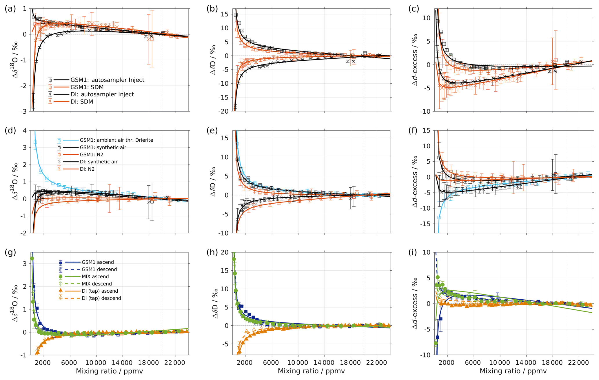
Figure A1(a–c) Comparison of the isotope composition–mixing ratio dependency of uncalibrated measurements with two different characterisation methods for (a) δ18O, (b) δD, and (c) d-excess. The measurements are carried out on instrument HIDS2254 (Picarro L2130-i), either with discrete injections using an autosampler (black symbols; experiment 2) or with continuous vapour streaming by using the SDM (red symbols; experiment 6) and using synthetic air as the carrier gas for both. The symbol and error bar represents the mean and standard deviation of the mean for the last three of a total of four injections for the measurement via the autosampler, and the mean and standard deviation of the last 2–5 min of a 20–30 min long sequence for the measurement via SDM. The solid line represents the fit using the same function as in Fig. 1. Panels (d–f) are the same as (a–c) but compare different carrier gases. The measurements are carried out on instrument HIDS2254 (Picarro L2130-i), with continuous vapour streaming via SDM (experiments 6–8). Two standard waters (GSM1 and DI) are tested with synthetic air (black symbol) and N2 (orange symbol). The standard water GSM1 is also tested with ambient air that is dried through Drierite (blue symbol). Panels (g–i) display the mixing ratio dependency of GSM1 (dark blue symbol), MIX (green symbol), and TAP water (orange symbol) with ascending (closed symbol) and descending (open symbol) mixing ratio sequences. Solid curves represent the fits for ascending mixing ratio sequences, and dashed curves represent the fits for descending mixing ratio sequences. All the measurements are uncalibrated and carried out with discrete injections using an autosampler with N2 as the carrier gas. The measurements for TAP and MIX are carried out on instrument HKDS2038 (Picarro L2140-i; experiments 9 and 11). The measurements for GSM1 are carried out on instrument HKDS2039 (Picarro L2140-i), and one outlier at around 500 ppmv has been excluded (experiment 15).
It is interesting to note that the result of the discrete liquid injections in February 2017 (experiment 1; Fig. 1) depicts a better agreement with that of the SDM in experiment 6 (comparison figure not shown). This indicates that the discrepancy in the results of the two vapour-generation methods could be due to the small instrument drift and the high measurement uncertainty at lower mixing ratios.
The experiments using N2 as dry gas supply (experiments 3 and 8) also give a similar isotope composition–mixing ratio dependency between the two vapour-generation methods (not shown), confirming that the isotope composition–mixing ratio dependency does not depend substantially on either of the two tested methods.
A2 Influence of dry gas supply
Next, we investigate whether the type of dry gas supply has an influence on the characterisation results. To this end, we test the characterisation method via the SDM on instrument HIDS2254 with a supply of synthetic air, a supply of N2, and a supply of dried ambient air through Drierite (experiments 6–8). The synthetic air and N2 are tested with two standard waters (GSM1 and DI), and the Drierite is tested with one standard water (GSM1).
For the mixing ratio dependency on δ18O, the measurement with Drierite disagrees strongly with those of synthetic air and N2 (Fig. A1e). As the mixing ratio decreases below about 7000 ppmv, the measured GSM1 with Drierite exhibits a fast-increasing positive deviation while that of synthetic air or N2 exhibits a rather flat dependency. The measurements with synthetic air and N2 largely show a similar shape. A small discrepancy exists below 15 000 ppmv, where the two standard waters measured with N2 exhibit a small negative offset (∼0.5 ‰). The mixing ratio dependencies on δD from all three types of the dry gas supply are in good agreement, despite a small (<1.5 ‰) offset between the measurement with synthetic air and that of N2 (Fig. A1e). The calculated d-excess follows the shape of δ18O, with different behaviours between the measurements with Drierite and those with synthetic air and N2 below about 7000 ppmv (Fig. A1f). The d-excess of the experiment with N2 exhibits a small positive offset (∼0.5 ‰) compared to the measurement with synthetic air. Overall, characterisation results with synthetic air and N2 exhibit a mixing ratio dependency in good agreement with the two investigated standard waters (GSM1 and DI). However, the characterisation result (for GSM1) with the Drierite differs significantly in δ18O and, thus, d-excess.
The characterisation method of liquid injections via an autosampler is also tested with synthetic air and N2. Again, the results exhibit a similar isotope composition–mixing ratio dependency from the two types of dry gas supply despite a small discrepancy for δ18O of GSM1 below 2000 ppmv and a relatively larger offset (0.5 ‰–1.3 ‰) for δ18O of DI below 10 000 ppmv (not shown). A test of synthetic air from a gas cylinder and dried ambient air from Drierite in the study of Aemisegger et al. (2012) also shows that the mixing ratio dependency is different for δ18O while being more similar for δD. The observed discrepancy in the δ18O deviation is possibly due to changes in the baseline of the spectrum around the and absorption peak, which is caused by slight differences in trace gas composition (Aemisegger et al., 2012; Rella et al., 2015).
A3 Influence from the measuring sequence
Finally, we investigate whether a measuring sequence with ascending or descending mixing ratio sequences influence the mixing ratio dependency characterisation. The mixing ratio dependencies of GSM1, MIX, and DI tap water that are characterised by ascending and descending mixing ratio sequences are shown in Fig. A1g–i. For both Δδ18O and ΔδD (Fig. A1g and h), the results from the two measuring sequences are in good agreement for all three waters, indicating that the influence of the measuring sequence is minor. However, there is a slightly detectable weaker mixing ratio dependency for the descending mixing ratio sequence (e.g. ΔδD for GSM1 and DI). One possible explanation for the slightly weaker dependency in the descending sequence is the memory effect from previous injections, e.g. some remaining water molecules would stick to the inner wall of the system (even after flushing the system with 12 injections at 20 000 ppmv) and still play a role during the characterisation measurements. If this is the case, the measurements from the descending mixing ratio sequence (starting with injections of higher mixing ratios at the beginning) would help to replace the remaining molecules through a molecular exchange and are therefore more likely to represent the true dependency behaviour. Nonetheless, the good agreement between the two measuring sequences indicates that the potential hysteresis effects, if any, are not substantial. The resulting mixing ratio dependencies for Δd-excess (Fig. A1i) exhibit an increasing positive deviation towards the low mixing ratios overall, except for one mixing ratio step of MIX and two mixing ratio steps of GSM1. This underlines the high sensitivity of d-excess measurements due to the increasing uncertainty of δ18O and δD values at very low mixing ratios.
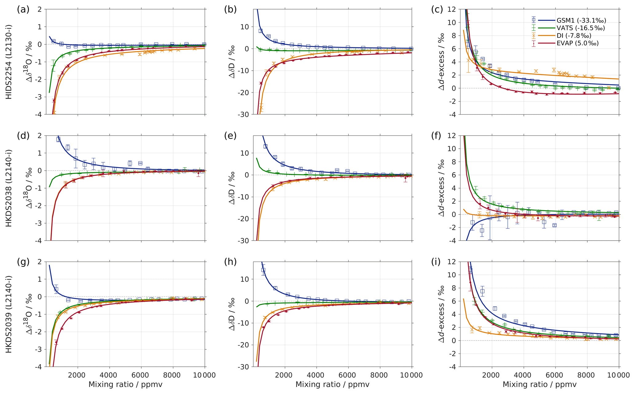
Figure A2Mixing ratio dependency of uncalibrated measurements for instruments (a–c) HIDS2254, (d–f) HKDS2038, and (g–i) HKDS2039. The measurements are carried out with discrete injections by using an autosampler with N2 as the carrier gas (experiments 3, 9, and 14). Only the data below 10 000 ppmv are shown. Symbols and solid lines indicate measurements and fits, respectively, as in Fig. 1.
It is worth noting that we have repeated three experiments for MIX (only results from one of the experiments are shown here). For one of the three experiments (not shown), the measurements for MIX below 2000 ppmv exhibit an interesting contrast in Δδ18O. The measurement at the lowest mixing ratio (around 500 ppmv) has constrained the mixing ratio dependency into slightly opposite directions. The contrast is not well understood. It is possible that this contrast stems from the fitting uncertainties due to the constraining points lacking at the low end of mixing ratios. The contrast is not observed for the repeated experiment with added mixing ratio steps (Fig. A1g; green). It is also possible that, for a standard in which the isotopic composition is close to a turning point in the correction surface (Sect. 5), hysteresis effects with opposing signs may become visible within the range of uncertainty. This can be also found, for example, in the small shift of the dependency shape in δD for VATS among the three analysers (Fig. A2b, e, and h; green curve). Further tests with more in-between standards, or a vapour-generation approach that does not suffer from memory, are needed to address this uncertainty in the dependency shape.
A4 Variations among CRDS analysers
To investigate the variations of the mixing ratio dependency between the individual instruments, we have repeated the same characterisation on three analysers (experiments 3, 9, and 14). The characterisation is carried out with four standard waters (GSM1, VATS, DI, and EVAP) by using liquid injections via an autosampler with N2 as the mixing dry gas.
The characterisation results for the three analysers are shown in Fig. A2. For Δδ18O, the positive deviation for GSM1 below 4000 ppmv on instrument HKDS2038 is about 0.2 ‰–1.8 ‰ stronger than that of the other two analysers (Fig. A2a, d, and g; blue). The mixing ratio dependency of VATS below 4000 ppmv is nearly flat on instrument HKDS2038 while exhibiting a substantial negative deviation for the other two analysers. The mixing ratio dependencies for the other two standard waters (DI and EVAP) are in good agreement among the three analysers. For ΔδD, the mixing ratio dependency of VATS below 2000 ppmv is slightly positive on instrument HKDS2038 while being nearly flat on the other two analysers (Fig. A2b, e, and h; green). The mixing ratio dependency for the other three standard waters (GSM1, DI, and EVAP) agree well among the three analysers. The calculated d-excess (Fig. A2c, f, and i) shows an increasing positive deviation towards the low end of the mixing ratio for almost all the standard waters measured on the three analysers except for DI and GSM1, which were measured on instrument HKDS2038 as their mixing ratio dependencies appear to be rather flat or even slightly negative.
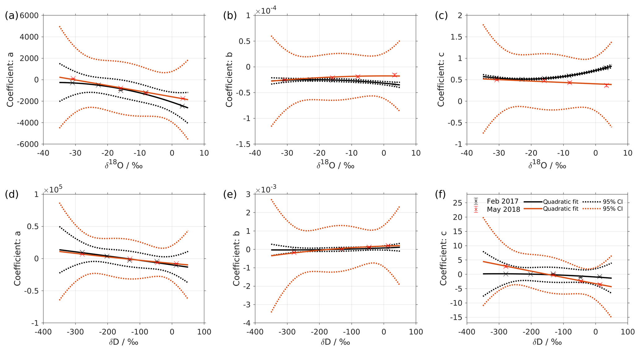
Figure A3Same as Fig. 2 but a comparison between results in February 2017 (black symbols; experiment 1) and May 2018 (red symbols; experiment 2). A larger, 95 % confidence interval for the fit of May 2018 (red dotted line) is due to the fewer data points available (only four standards measured).
Despite the minor difference in the magnitude of the deviations, it is clear that the isotope composition–mixing ratio dependency exists in all three analysers investigated here. The behaviour of the dependency is, to the first order, in good agreement across the analysers. For the standard waters with relatively depleted isotope compositions, the measurements of all three analysers exhibit a mixing ratio dependency, where the isotopic value increases as the mixing ratio decreases. For the standard waters with relatively enriched isotope compositions, the measurements exhibit a reversed mixing ratio dependency.
A5 Long-term stability
To quantify the long-term stability of the isotope composition–mixing ratio dependency, we examine the temporal change of the fitting coefficients (aδ, bδ, and cδ) in Eq. (4). Figure A3 shows the fitting coefficients for the mixing ratio dependency characterised by liquid injections on instrument HIDS2254 in February 2017 (experiment 1; black line) and in May 2018 (experiment 2; red line). For the characterisation in May 2018, only four standard waters are measured; this results in a fit with a relatively large, 95 % confidence interval. In this context the change over time is considered insignificant if the coefficients (and their fitted curve) from the characterisation in May 2018 are within the 95 % confidence bounds for the fitted curve from the characterisation in February 2017.
For the mixing ratio dependency on δ18O, the change of coefficient a is insignificant. However, it is worth noting that the fitting coefficient a, with respect to standard GSM1 (Fig. A3a; the first data point), changes slightly from negative to positive. This small change results in an opposite mixing ratio dependency shape at a low mixing ratio. The change of the mixing ratio dependency for GSM1 partly reflects on the sensitivity of the instrument to a certain range of isotope compositions and partly on the uncertainty arising from both low instrument precision and a lack of measurements at low mixing ratios. The changes of coefficients b and c are substantial for the standard waters of relatively high δ18O (Fig. A3b, c). A less negative b and a less positive c reflects a weaker mixing ratio dependency in May 2018. For the mixing ratio dependency on δD, a reasonable agreement is exhibited for all three fitting coefficients (Fig. A3d, e, and f); this points to the same basic shape of the mixing ratio dependency on δD after a 15-month period.
A repeated characterisation determined via the SDM with standard water DI in July 2016, February 2018, and June 2018 (experiments 4, 5, and 6) indicates that the mixing ratio dependency for standard water DI is still consistent after nearly 2 years (not shown). The mixing ratio dependencies of the three standard waters (GSM1, VATS, and DI) determined by liquid injections via an autosampler (experiments 9 and 10) and the other three standard waters (NEEM, GV, and BERM) via manual injections in instrument HKDS2038 (experiments 12 and 13) indicate a consistent isotope composition–mixing ratio dependency after a running of 1 year and 1 month respectively (not shown). Overall, the stability tests indicate that the isotope composition–mixing ratio dependency of each analyser is, to the first order, stable on a long-term basis (1–2 years).
Since we only have 5 available data points to fit in Eq. (5), the resultant 95 % confidence interval of the fit is relatively broad (black dotted line; Fig. 2). This broad confidence interval results in a relatively large standard deviation for the isotopic deviation (Δδ). For example, the resultant standard deviation for Δδ at 2000 ppmv is about 0.20 ‰, 2.69 ‰, and 3.13 ‰ for δ18O, δD, and d-excess respectively. To reduce this large standard deviation for Δδ, we use a bootstrapping approach (Efron, 1979) to estimate the fitting uncertainty in Eq. (5).
The bootstrapping approach can be explained by considering, for example, the coefficient a. For each individual observation of a, we generate 1000 random values under a normal distribution, with the mean and standard deviation being those of each available observation. We now obtain five sets of 1000 random values since we have 5 a from five standard waters. Then, we sample 1 value from each set of the 1000 random values and fit those 5 sampled values using Eq. (5). Finally, we repeat this process 1000 times, thus obtaining 1000 fits. The standard deviation of the 1000 fits is the standard deviation that is adopted here (blue dotted line; Fig. 2).
In this way, the standard deviations estimated for the coefficients a, b, and c are lowered to about 15, , and for δ18O and 100, , and 0.1 for δD respectively. This, in turn, substantially reduces the resultant standard deviation for Δδ. For example, the standard deviation for Δδ at 2000 ppmv is reduced by a factor of 20, which is about 0.01 ‰, 0.11 ‰, and 0.14 ‰ for δ18O, δD, and d-excess respectively.
In the following, we derive the analytical solution for δcor in Eq. (7) at the reference mixing ratio (i.e. 20 000 ppmv). The derivation applies to both δ18O and δD.
The coefficients a(δcor), b(δcor), and c(δcor) are given according to Eq. (5) as follows:
By substituting Eq. (C1) into Eq. (7) and rearranging the terms, we calculate the following:
Equation (C2) is a quadratic equation with its only physical solution being the following:
The coefficients m, n, and k are already obtained from the fits in Eq. (5). When given a measured mixing ratio, h, and the corresponding isotope composition, δmeas, we can obtain the isotope composition at 20 000 ppmv, which is δcor according to the solution Eq. (C3).
Data used in the generation of the figures are attached as a Supplement to this article.
The supplement related to this article is available online at: https://doi.org/10.5194/amt-13-3167-2020-supplement.
YW and HS designed the study jointly. Experiments and data analysis was led by YW with contributions from AT. All authors contributed to the writing of the paper.
The authors declare that they have no conflict of interest.
The authors wish to thank Iris Thurnherr, Franziska Aemisegger, and Pascal Graf from the Institute for Atmospheric and Climate Sciences, ETH Zurich; Hans Christian Steen-Larsen and Sonja Wahl from the Geophysical Institute, University of Bergen; and Jean-Lionel Lacour and Tomas Foldes for the valuable discussions. We are grateful to Arny Erla Sveinbjornsdottir from the isotope laboratory of the University of Iceland for providing the UI standard waters. Jarle Berntsen from the Department of Mathematics at the University of Bergen is acknowledged for helping to identify a suitable fitting function. We are grateful to the scientists and other personnel who made the measurements during the Iceland–Greenland Seas Project campaign of 2018 possible. We thank Chris Rella for providing valuable comments on our paper. We would also like to express our gratitude to the editor and the three anonymous reviewers whose valuable comments have significantly helped to improve the clarity of this paper.
This research has been supported by the Research Council of Norway (SNOWPACE (grant no. 262710) and FARLAB (grant no. 245907)).
This paper was edited by Christof Janssen and reviewed by three anonymous referees.
Aemisegger, F., Sturm, P., Graf, P., Sodemann, H., Pfahl, S., Knohl, A., and Wernli, H.: Measuring variations of δ18O and δ2H in atmospheric water vapour using two commercial laser-based spectrometers: an instrument characterisation study, Atmos. Meas. Tech., 5, 1491–1511, https://doi.org/10.5194/amt-5-1491-2012, 2012. a, b, c, d, e, f
Baertschi, P.: Absolute 18O content of standard mean ocean water, Earth Planet. Sc. Lett., 31, 341–344, 1976. a, b
Bailey, A., Noone, D., Berkelhammer, M., Steen-Larsen, H. C., and Sato, P.: The stability and calibration of water vapor isotope ratio measurements during long-term deployments, Atmos. Meas. Tech., 8, 4521–4538, https://doi.org/10.5194/amt-8-4521-2015, 2015. a, b
Bastrikov, V., Steen-Larsen, H. C., Masson-Delmotte, V., Gribanov, K., Cattani, O., Jouzel, J., and Zakharov, V.: Continuous measurements of atmospheric water vapour isotopes in western Siberia (Kourovka), Atmos. Meas. Tech., 7, 1763–1776, https://doi.org/10.5194/amt-7-1763-2014, 2014. a
Bonne, J.-L., Masson-Delmotte, V., Cattani, O., Delmotte, M., Risi, C., Sodemann, H., and Steen-Larsen, H. C.: The isotopic composition of water vapour and precipitation in Ivittuut, southern Greenland, Atmos. Chem. Phys., 14, 4419–4439, https://doi.org/10.5194/acp-14-4419-2014, 2014. a, b, c, d, e, f, g
Bonne, J.-L., Behrens, M., Meyer, H., Kipfstuhl, S., Rabe, B., Schönicke, L., Steen-Larsen, H. C., and Werner, M.: Resolving the controls of water vapour isotopes in the Atlantic sector, Nat. Commun., 10, 1–10, 2019. a
Crosson, E. R.: A cavity ring-down analyzer for measuring atmospheric levels of methane, carbon dioxide, and water vapor, Appl. Phys. B, 92, 403–408, 2008. a
Dansgaard, W.: The abundance of O18 in atmospheric water and water vapour, Tellus, 5, 461–469, 1953. a
Dansgaard, W.: The O18-abundance in fresh water, Geochim. Cosmochim. Ac., 6, 241–260, 1954. a
Dansgaard, W.: Stable isotopes in precipitation, Tellus, 16, 436–468, 1964. a
Efron, B.: Bootstrap Methods: Another Look at the Jackknife, Annals of Statistics, 7, 1–26, 1979. a, b
Gat, J. R.: Oxygen and hydrogen isotopes in the hydrologic cycle, Annu. Rev. Earth Planet. Sci., 24, 225–262, 1996. a
Goldenstein, C. S., Miller, V. A., Spearrin, R. M., and Strand, C. L.: SpectraPlot.com: Integrated spectroscopic modeling of atomic and molecular gases, J. Quant. Spectrosc. Ra., 200, 249–257, https://doi.org/10.1016/j.jqsrt.2017.06.007, 2017. a
Gupta, P., Noone, D., Galewsky, J., Sweeney, C., and Vaughn, B. H.: Demonstration of high-precision continuous measurements of water vapor isotopologues in laboratory and remote field deployments using wavelength-scanned cavity ring-down spectroscopy (WS-CRDS) technology, Rapid Comm. Mass Spectr., 23, 2534–2542, 2009. a
Hagemann, R., Nief, G., and Roth, E.: Absolute isotopic scale for deuterium analysis of natural waters. Absolute D/H ratio for SMOW 1, Tellus, 22, 712–715, 1970. a
International Atomic Energy Agency: Reference Sheet for VSMOW2 and SLAP2 International Measurement Standards, IAEA, Vienna, 8 pp. (Rev 1 dated 11 July 2017), 2009. a
Johnson, J. E. and Rella, C. W.: Effects of variation in background mixing ratios of N2, O2, and Ar on the measurement of δ18O–H2O and δ2H–H2O values by cavity ring-down spectroscopy, Atmos. Meas. Tech., 10, 3073–3091, https://doi.org/10.5194/amt-10-3073-2017, 2017. a, b, c, d
Kerstel, E.: Isotope ratio infrared spectrometry, in: Handbook of stable isotope analytical techniques, chapter 34, edited by: de Groot, P. A., pp. 759–787, ISBN 978-0-444-51114-0, Elsevier, Amsterdam, 2004. a
Kerstel, E. and Gianfrani, L.: Advances in laser-based isotope ratio measurements: selected applications, Appl. Phys. B, 92, 439–449, 2008. a
Kurita, N., Newman, B. D., Araguas-Araguas, L. J., and Aggarwal, P.: Evaluation of continuous water vapor δD and δ18O measurements by off-axis integrated cavity output spectroscopy, Atmos. Meas. Tech., 5, 2069–2080, https://doi.org/10.5194/amt-5-2069-2012, 2012. a
Lis, G., Wassenaar, L., and Hendry, M.: High-precision laser spectroscopy D/H and 18O∕16O measurements of microliter natural water samples, Anal. Chem., 80, 287–293, 2008. a
Mook, W. G. and De Vries, J. J.: Environmental isotopes in the hydrological cycle: principles and applications, in: Environmental Isotopes in the Hydrological Cycle – Principles and Applications, International Hydrological Programme (IHP-V), Technical Documents in Hydrology, IAEA/UNESCO, 1, 30–31, 2001. a
O'Keefe, A. and Deacon, D. A.: Cavity ring-down optical spectrometer for absorption measurements using pulsed laser sources, Rev. Sci. Instr., 59, 2544–2551, 1988. a
Picarro Inc.: Calibration guide for Picarro analyzers, Rev 1., 18 pp., 2017. a
Rella, C. W., Hoffnagle, J., He, Y., and Tajima, S.: Local- and regional-scale measurements of CH4, δ13CH4, and C2H6 in the Uintah Basin using a mobile stable isotope analyzer, Atmos. Meas. Tech., 8, 4539–4559, https://doi.org/10.5194/amt-8-4539-2015, 2015. a, b, c, d, e, f, g, h, i
Renfrew, I. A., Pickart, R. S., Våge, K., Moore, G. W. K., Bracegirdle, T. J., Elvidge, A. D., Jeansson, E., Lachlan-Cope, T., McRaven, L. T., Papritz, L., Reuder, J., Sodemann, H., Terpstra, A., Waterman, S., Valdimarsson, H., Weiss, A., Almansi, M., Bahr, F., Brakstad, A., Barrell, C., Brooke, J. K., Brooks, B. J., Brooks, I. M., Brooks, M. E., Bruvik, E. M., Duscha, C., Fer, I., Golid, H. M., Hallerstig, M., Hessevik, I., Huang, J., Houghton, L., Jónsson, S., Jonassen, M., Jackson, K., Kvalsund, K., Kolstad, E. W., Konstali, K., Kristiansen, J., Ladkin, R., Lin, P., Macrander, A., Mitchell, A., Olafsson, H., Pacini, A., Payne, C., Palmason, B., Pérez-Hernández, M. D., Peterson, A. K., Petersen, G. N., Pisareva, M. N., Pope, J. O., Seidl, A., Semper, S., Sergeev, D., Skjelsvik, S., Søiland, H., Smith, D., Spall, M. A., Spengler, T., Touzeau, A., Tupper, G., Weng, Y., Williams, K. D., Yang, X., and Zhou, S.: The Iceland Greenland Seas Project, B. Am. Meteorol. Soc., 100, 1795–1817, https://doi.org/10.1175/BAMS-D-18-0217.1, 2019. a, b, c
Schmidt, M., Maseyk, K., Lett, C., Biron, P., Richard, P., Bariac, T., and Seibt, U.: Concentration effects on laser-based δ18O and δ2H measurements and implications for the calibration of vapour measurements with liquid standards, Rapid Commun. Mass Spectr., 24, 3553–3561, 2010. a
Sodemann, H., Aemisegger, F., Pfahl, S., Bitter, M., Corsmeier, U., Feuerle, T., Graf, P., Hankers, R., Hsiao, G., Schulz, H., Wieser, A., and Wernli, H.: The stable isotopic composition of water vapour above Corsica during the HyMeX SOP1 campaign: insight into vertical mixing processes from lower-tropospheric survey flights, Atmos. Chem. Phys., 17, 6125–6151, https://doi.org/10.5194/acp-17-6125-2017, 2017. a, b, c
Steen-Larsen, H. C., Johnsen, S. J., Masson-Delmotte, V., Stenni, B., Risi, C., Sodemann, H., Balslev-Clausen, D., Blunier, T., Dahl-Jensen, D., Ellehøj, M. D., Falourd, S., Grindsted, A., Gkinis, V., Jouzel, J., Popp, T., Sheldon, S., Simonsen, S. B., Sjolte, J., Steffensen, J. P., Sperlich, P., Sveinbjörnsdóttir, A. E., Vinther, B. M., and White, J. W. C.: Continuous monitoring of summer surface water vapor isotopic composition above the Greenland Ice Sheet, Atmos. Chem. Phys., 13, 4815–4828, https://doi.org/10.5194/acp-13-4815-2013, 2013. a
Steen-Larsen, H. C., Sveinbjörnsdottir, A. E., Peters, A. J., Masson-Delmotte, V., Guishard, M. P., Hsiao, G., Jouzel, J., Noone, D., Warren, J. K., and White, J. W. C.: Climatic controls on water vapor deuterium excess in the marine boundary layer of the North Atlantic based on 500 days of in situ, continuous measurements, Atmos. Chem. Phys., 14, 7741–7756, https://doi.org/10.5194/acp-14-7741-2014, 2014. a
Steig, E. J., Gkinis, V., Schauer, A. J., Schoenemann, S. W., Samek, K., Hoffnagle, J., Dennis, K. J., and Tan, S. M.: Calibrated high-precision 17O-excess measurements using cavity ring-down spectroscopy with laser-current-tuned cavity resonance, Atmos. Meas. Tech., 7, 2421–2435, https://doi.org/10.5194/amt-7-2421-2014, 2014. a, b, c, d, e, f, g, h
Sturm, P. and Knohl, A.: Water vapor δ2H and δ18O measurements using off-axis integrated cavity output spectroscopy, Atmos. Meas. Tech., 3, 67–77, https://doi.org/10.5194/amt-3-67-2010, 2010. a
Thurnherr, I., Kozachek, A., Graf, P., Weng, Y., Bolshiyanov, D., Landwehr, S., Pfahl, S., Schmale, J., Sodemann, H., Steen-Larsen, H. C., Toffoli, A., Wernli, H., and Aemisegger, F.: Meridional and vertical variations of the water vapour isotopic composition in the marine boundary layer over the Atlantic and Southern Ocean, Atmos. Chem. Phys., 20, 5811–5835, https://doi.org/10.5194/acp-20-5811-2020, 2020. a, b
Wen, X. F., Lee, X., Sun, X. M., Wang, J. L., Tang, Y. K., Li, S. G., and Yu, G. R.: Intercomparison of four commercial analyzers for water vapor isotope measurement, J. Atmos. Ocean. Technol., 29, 235–247, https://doi.org/10.1175/JTECH-D-10-05037.1, 2012. a, b
- Abstract
- Introduction
- Methods and data
- Isotope composition–mixing ratio dependency
- Robustness and temporal stability of the isotope composition–mixing ratio dependency
- Correction framework
- Impact of the isotope composition–mixing ratio dependency correction
- Discussion
- Final remarks and recommendations
- Appendix A: Robustness and temporal stability
- Appendix B: Fitting uncertainty estimated using a bootstrapping approach
- Appendix C: Analytical solution for δcor
- Data availability
- Author contributions
- Competing interests
- Acknowledgements
- Financial support
- Review statement
- References
- Supplement