2.1 SRON multimode retrieval algorithm

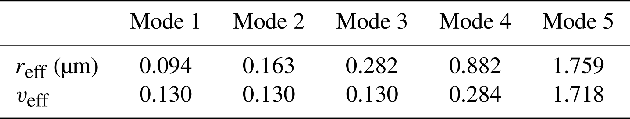
In this paper, we employ the SRON aerosol retrieval algorithm in a multimode setup (Fu and Hasekamp, 2018). In principle, the idea of the multimode approach is that instead of fitting the size distribution parameters (the effective radius r_eff and the effective variance v_eff) of two modes, one aims to fit the size distribution with a larger number of modes for which r_eff and v_eff are fixed. The advantage of this approach is that it makes the inversion problem more linear since r_eff and v_eff tend to make the inversion highly nonlinear. Another advantage is that the multimode approach has more freedom in fitting different shapes of the size distribution if the number of chosen modes is sufficiently large. In this paper, multimode retrievals based on five modes are used, and the aerosol size distribution is described in Table 1 (Fu and Hasekamp, 2018). We consider modes 1–3 together as the fine mode and modes 4 and 5 together as the coarse mode. To account for spectral dependence, we describe the refractive index m for the fine and coarse mode as $m\left(\mathit{\lambda }\right)={\sum }_{k=\mathrm{1}}^{n_{\mathit{\alpha }}}{\mathit{\alpha }}_k{m}^k\left(\mathit{\lambda }\right)$, where m^k(λ) represents prescribed refractive indices as a function of wavelength and α_k represents coefficients to be determined in the retrieval (see below). Both the real part and imaginary part of refractive indices are represented in this way. Here, we base the spectral dependence of the refractive index on the standard types of D'Almeida et al. (1991) (inorganic–sulfate, black carbon, and dust). The coefficients α_k are the real numbers between 0 and 1 and are defined as weighting factors to combine the refractive index spectra for different aerosol components, e.g., DUST, water (H₂O), black carbon (BC), and inorganic matter (INORG). In this study, we set n_α=2 and assume that the spectral dependence of the fine-mode and the coarse-mode refractive indices can be respectively described by INORG+BC and DUST+INORG. Note that this assumption is flexible and can be updated according to the information content of the measurement. Spectra based on principal component analysis (PCA) can also be used as in Wu et al. (2015). The standard refractive index spectra are only used to describe the spectral dependence as the MAP measurements do not contain sufficient information to retrieve the refractive index for each wavelength separately. Nonspherical aerosols are described as a size–shape mixture of randomly oriented spheroids (Hill et al., 1984; Mishchenko et al., 1997). We use the Mie- and T-matrix-improved geometrical optics database by Dubovik et al. (2006) along with their proposed spheroid aspect ratio distribution for computing optical properties for a mixture of spheroids and spheres. The aerosol parameters included in the retrieval state vector x are the aerosol column numbers for the five modes (Table 1), two coefficients (inorganic, black carbon) for the fine-mode refractive index, two coefficients (inorganic, dust) for the coarse-mode refractive index, the fraction of spherical particles (assumed the same for all modes), and the central height of a Gaussian aerosol height distribution (assumed the same for all modes).

Table 1Definition of the effective radius (r_eff) and the effective variance (v_eff) in the SRON five-mode retrieval.

Download Print Version | Download XLSX

For the surface reflection matrix we use (Rahman et al., 1993; Litvinov et al., 2011; Xu et al., 2017)

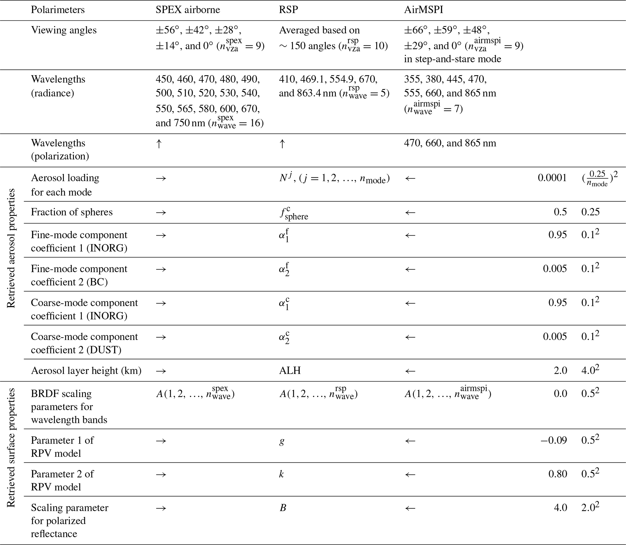
where k is a parameter that varies between 0 and 1. This parameter controls the slope of the reflectance with respect to the illumination and view angles (Rahman et al., 1993). D is the null matrix except D₁₁=1. The first part in Eq. (1) accounts for the bidirectional reflectance distribution function (BRDF) parameterized by the Rahman–Pinty–Verstraete (RPV) model (Rahman et al., 1993). The pairs (θ₀, ϕ₀) and (θ_v, ϕ_v) respectively denote the solar and viewing zenith and azimuth angles. μ_in and μ_out are respectively the cosines of incoming and outgoing angles. g is the asymmetry parameter of the Henyey–Greenstein phase function F(g,Θ). Θ is the scattering angle. 1+R(G) is an approximation of the hot spot effect (Rahman et al., 1993), where $G=\sqrt{{\tan }^{\mathrm{2}}{\mathit{\theta }}_{\mathrm{0}}+{\tan }^{\mathrm{2}}{\mathit{\theta }}_{\mathrm{v}}-\mathrm{2}\tan {\mathit{\theta }}_{\mathrm{0}}\tan \left|{\mathit{\theta }}_{\mathrm{v}}\right|\cos \left({\mathit{\varphi }}_{\mathrm{v}}-{\mathit{\varphi }}_{\mathrm{0}}\right)}$ and $R\left(G\right)=\frac{\mathrm{1}-A\left(\mathit{\lambda }\right)}{\mathrm{1}+G}$. The second part in Eq. (1) accounts for the surface polarized reflectance, for which we use the model proposed by Maignan et al. (2009). R_pol is expressed by Eq. (2) (as stated by Eq. 31 in Litvinov et al., 2011). Here, B is a scaling parameter (band independent). F_p(m,Θ) is the element F₂₁ of the Fresnel scattering matrix with refractive index m. Parameter ν is taken based on the atmospherically resistant vegetation index (ARVI) (Kaufman and Tanre, 1992). Here we use ν=0.6. Based on Eqs. (1) and (2), We include A(λ) at each measured wavelength and k, g, and B as fit parameters in the state vector. In this paper, we perform aerosol retrievals from SPEX airborne, RSP, and AirMSPI, and the state vectors corresponding to these three polarimeters are listed in Table 2.

Table 2Viewing angles and wavelengths used in retrievals among SPEX airborne, RSP, and AirMSPI, as well as the retrieved parameters from them. Prior values and weighting factors for the state vector are also listed in the table. In this paper, five-mode retrieval is used, and thus n_mode=5. The arrows →, ←, or ↑ indicate the same value with the arrow direction. The prior value and weighting factor of aerosol loading for each mode are calculated based on Mie theory using the prior information of AOD from the table (listed in the row of aerosol loading).

Download Print Version | Download XLSX

The measurement vector y contains the measured radiances (sun normalized) and degree of linear polarization (DoLP) values at the different wavelengths and viewing angles. To retrieve the state vector from the measurements, a damped Gauss–Newton iteration method with Phillips–Tikhonov regularization is employed (Hasekamp et al., 2011; Fu and Hasekamp, 2018). The inversion algorithm finds the solution $\widehat{\mathit{x}}$, which solves the minimization-optimization problem,

Here, F is the forward model that simulates the measurement for a given state vector x. F consists of a radiative transfer model, for which we use the SRON radiative transfer model LINTRAN (Landgraf et al., 2001; Hasekamp and Landgraf, 2002, 2005; Schepers et al., 2014). All the radiative transfer calculations are performed for a model atmosphere that includes Rayleigh scattering, scattering and absorption by aerosols, and gas absorption. Rayleigh scattering cross sections are used from Bucholtz (1995). The forward model simulates Stokes parameters I, Q, and U at the height of the observation (e.g., ∼20 km for NASA ER-2 in this paper) for given optical properties (scattering and absorption optical thickness and scattering phase matrix for each vertical layer of the model atmosphere; 15 layers of the atmosphere are assumed). The other part of the forward model computes the optical properties from the aerosol microphysical properties using the tabulated kernels of Dubovik et al. (2006) for a mixture of spheroids and spheres.

Since the forward model is nonlinear the inversion problem has to be solved iteratively by replacing the forward model in each iteration step by its linear approximation,

Here, K is the Jacobian matrix (with $K_{ij}=\frac{\partial F_i}{\partial x_j}\left({\mathit{x}}_n\right)$), which contains the derivatives of the forward model with respect to each variable in the state vector x. Therefore, the optimization problem (Eq. 3) is reduced to

where $\stackrel{\mathrm{̃}}{\mathbf{K}}={\mathbf{S}}_y^{-\frac{\mathrm{1}}{\mathrm{2}}}{\mathbf{KW}}^{\frac{\mathrm{1}}{\mathrm{2}}}$, $\stackrel{\mathrm{̃}}{\mathit{x}}={\mathbf{W}}^{-\frac{\mathrm{1}}{\mathrm{2}}}\mathit{x}$, and $\stackrel{\mathrm{̃}}{\mathit{y}}={\mathbf{S}}_y^{-\frac{\mathrm{1}}{\mathrm{2}}}\left(\mathit{y}-\mathbf{F}\left({\mathit{x}}_n\right)\right)$. x_a is the a priori state vector, W is a weighting matrix that ensures that all state vector parameters range within the same order of magnitude (Hasekamp et al., 2011), and S_y is the measurement error covariance matrix. Table 2 shows the values of x_a for aerosol and surface parameters. W is a diagonal matrix, and its diagonal values are also shown in Table 2 (in the “weight” column). The solution of Eq. (5) is given by

Λ is a filtering–damping factor, which limits the step size for each iteration of the state vector. In this way, we use a Gauss–Newton scheme with reduced step size to avoid diverging retrievals (Hasekamp et al., 2011). The filter factor Λ values between 0 and 1. The regularization parameter γ² in Eq. (3) is chosen optimally (for each iteration) from different values (five values from 0.1 to 5) by evaluating the goodness of fit using a simplified (fast) forward model. In the SRON aerosol algorithm, the first guess is obtained before the full inversion retrieval using a multimode lookup table (LUT), which is based on tabulated RT calculations for each mode. The precalculated LUT is used as input for an approximate forward model in the LUT retrieval. Here, single-scattering is computed exactly as its computational cost is negligible. The fit parameters in the LUT retrieval are the aerosol column numbers for each mode and the surface parameters. For the first guess of the refractive index we use a fixed value of 1.45 for all modes. For further details we refer to Fu and Hasekamp (2018).

We use the goodness of fit (χ²) to decide whether the retrievals have successfully converged:

Here, n_meas is the total number of measurements (multi-angle and multispectral radiance and DoLP) for each pixel. We consider valid retrievals those that achieve a χ² smaller than an empirically chosen threshold ${\mathit{\chi }}_{\max }^{\mathrm{2}}$. This filter rejects cases in which the forward model is not able to fit the measurements, e.g., because of cloud-contaminated pixels (Stap et al., 2015, 2016) or corrupted measurements (Hasekamp et al., 2011), and cases in which the first-guess state vector deviates too much from the truth (Di Noia et al., 2015).

2.2 Fine-mode and coarse-mode effective radius

According to Eq. (2.53) in Hansen and Travis (1974), the effective radius is defined as follows:

where n(r)dr is the number of particles with a radius between r and r+dr; r_min and r_max are the particle radius for the smallest and largest particles.

In this study, a five-mode retrieval is used. The effective radius for multiple modes together ($r_{\mathrm{eff}}^{\mathrm{m}}$) is calculated from the different fixed modes by

where n^m is the number of modes grouped together. For the five-mode retrievals in this study, we compute r_eff for the fine mode (modes 1–3 together) and coarse mode (modes 4 and 5 together).

2.3 Aerosol depolarization ratio and aerosol lidar ratio

The aerosol lidar properties are related to the aerosol scattering matrix. For some general assumptions, including (i) scattering by an assembly of randomly oriented particles each having a plane of symmetry, (ii) scattering by an assembly containing particles and their mirror particles in equal numbers with random orientations, and (iii) Rayleigh scattering with or without depolarization effects, the aerosol scattering matrix has a simplified block-diagonal structure (Bottiger et al., 1980; Mishchenko, 2014):

where Θ is the scattering angle and F₁₁ is the phase function for total radiance.

The aerosol (linear) depolarization ratio is defined as

which is adapted from Eq. (3) in Mishchenko et al. (2016). We use Eq. (10) to compute an aerosol depolarization ratio from the aerosol properties of the MAPs and compare this to the vertically integrated value measured by HSRL-2, which is calculated by

where i=0 corresponds to the bin closet to the surface, and i=n_bin corresponds to the bin closet to the aircraft. The aerosol backscatter coefficient (${\mathit{\beta }}_{\mathrm{b}}^{\mathrm{hsrl}}\left(i\right)$) for each bin is used as the weighting parameter. δ^hsrl(i) is first transformed to ${\widehat{\mathit{\delta }}}^{\mathrm{hsrl}}\left(i\right)$, which is because ${\widehat{\mathit{\delta }}}^{\mathrm{hsrl}}\left(i\right)$ mixes linearly like backscatter, but δ^hsrl(i) does not (Burton et al., 2014).

In our retrieval algorithm we assume that for aerosols the single-scattering albedo ω and F₁₁ do not depend on altitude. In that case, using ω and F₁₁(180^∘), we compute the vertically integrated aerosol extinction-to-backscatter ratio, i.e., the aerosol lidar ratio, for a MAP by

which is adapted from Eq. (4) in Lopes et al. (2013). This can be compared to the corresponding value from HSRL-2:

which is adapted from Eq. (28) in Stamnes et al. (2018). Here ${\mathit{\beta }}_{\mathrm{e}}^{\mathrm{hsrl}}\left(i\right)$ denotes the extinction coefficient for each bin.

3.1 RSP

RSP (Cairns et al., 1999) started to operate on the NASA ER-2 in 2010 and has flown on a number of other airplanes since 2001 (Cairns et al., 2003). Multi-viewing capability over a large along-track angular range and at many viewing angles (∼150) is obtained using a scanning mirror. Due to the fact that some viewing angles are blocked by the aircraft, the angular range of RSP on the ER-2 is restricted to −40 to 60^∘. The Stokes parameters Q and U are analyzed in separate refractive telescopes using Wollaston prisms, followed by dichroic beam splitters. The RSP instrument is equipped with an in-flight calibration system, and the accuracy for the DoLP is better than 0.002 (Knobelspiesse et al., 2019), providing a benchmark (in DoLP) for other MAPs. Aerosol retrievals from RSP have been performed, amongst others, by Waquet et al. (2009), Wu et al. (2015), Wu et al. (2016), Di Noia et al. (2017), Stamnes et al. (2018), and Gao et al. (2019).

A complicating factor for using RSP measurements in aerosol retrievals over inhomogeneous land surfaces is that different viewing angles have different ground pixel size and may look at slightly shifted scenes on the ground. To partly overcome this problem we use (1) the approach of Wu et al. (2015) and construct RSP pixels that represent a 5 km along-track running average, as well as (2) the (moving average) approach of Di Noia et al. (2017) to select 10 viewing angles covering a broad viewing angle range (over the total RSP viewing angles), and convolve RSP measurements at each selected angle with an average of five angles. In this sense, although averaged measurements of 10 viewing angles are input to the retrieval algorithm, they are constructed from original RSP measurements at 50 angles. The viewing angles and wavelengths used in retrievals are summarized in Table 2. It should be noted that theoretically the shortwave infrared (SWIR) bands of RSP 1590 and 2250 nm would provide extra constraints for the characterization of coarse-mode aerosols. For the ACEPOL campaign, however, we found no improvement by including the SWIR bands and even slightly worse results (compared to AERONET and HSRL-2) in some cases. A possible explanation is that our assumption that the directional property of surface reflection is spectrally neutral does not hold over the full RSP wavelength range. Another explanation may be that the SWIR channels are affected by gas absorption, which we could not perfectly correct for.

3.2 AirMSPI

AirMSPI (Diner et al., 2013) started to operate on the NASA ER-2 in October 2010. AirMSPI is an eight-band push-broom camera, which measures linear polarization in the 470, 660, and 865 nm bands. AirMSPI employs a photoelastic modulator-based polarimetric imaging technique to enable accurate measurements of the degree of linear polarization (DoLP) in addition to intensity. The instrument is mounted on a gimbal to acquire multi-angular observations in the range of ±67^∘. AirMSPI has two principal observing modes: (1) step-and-stare, whereby 11 km×11 km targets are observed at a discrete set of view angles with a spatial resolution of ∼10 m, and (2) continuous sweep, whereby the camera slews back and forth along the flight track at ±65^∘ to acquire wide area coverage (11 km swath at nadir, target length 108 km). The spatial resolution is ∼25 m. Aerosol retrievals from AirMSPI have been performed by Xu et al. (2017, 2018, 2019). In this study, only the step-and-stare measurements have been used as they provide a multi-angle view of the same ground scene. The nine viewing angles and seven wavelengths used in retrievals are summarized in Table 2. Following Xu et al. (2017), for AirMSPI we aggregate individual ground pixels to a 1 km×1 km spatial grid in order to be less affected by surface inhomogeneity and its effect on the angular co-registration.

3.3 SPEX airborne

SPEX airborne performed its first (engineering) flight on the ER-2 in 2016. ACEPOL was the first full science campaign. The instrument employs the spectral modulation technique (Snik et al., 2009) to accurately measure the degree of linear polarization (DoLP) in the spectral range 400–800 nm with a spectral resolution of 10–20 nm and the intensity at a higher spectral resolution of 2–3 nm. A ground-based version of SPEX has performed upward-looking measurements from the ground, which have been used to successfully retrieve aerosol microphysical and optical properties by van Harten et al. (2014) and Di Noia et al. (2015). For ACEPOL, Smit et al. (2019) performed a comparison between SPEX airborne and RSP for radiance and DoLP measurements at 410, 470, 550, and 670 nm. They found very good agreement between SPEX airborne and RSP at 550 and 670 nm, whereas the agreement gets worse towards smaller wavelengths. In this study, the nine viewing angles and 16 wavelengths used in retrievals are summarized in Table 2. The measurement at each wavelength represents an average of a 10 nm wide spectral region. We leave out the shortest wavelengths because of less good agreement with RSP and the wavelengths >750 nm because of order overlap of the grating. Each SPEX viewport has a moderate swath of ∼6^∘ (Smit et al., 2019) in the across-track direction, which translates to a projected field of view from 2.4 km at nadir to 4.5 km at the fore and aft viewports when the instrument is operated at the typical altitude of ER-2. Conceptually, the instrument acts as nine separate push-broom spectrometers, which produce nine overlapping strips of data on the ground. In this way, a multi-angular view is obtained of ground scenes when the aircraft flies over it. The spatial sampling of the L1C product is chosen as 1 km×1 km (across × along-track), which is driven by the L1B spatial resolution of the outer viewports.

3.4 HSRL-2 data

The NASA Langley HSRL-2 instrument, operational since 2012, is a successor to the NASA Langley airborne HSRL-1 instrument, which was described by Hair et al. (2008) and Burton et al. (2012), then validated by Rogers et al. (2009). HSRL-2 uses the HSRL technique to independently measure aerosol extinction and backscatter at 355 nm (Burton et al., 2018) and 532 nm as well as the standard backscatter technique to measure aerosol backscatter at 1064 nm (Müller et al., 2014). It is polarization sensitive at all three wavelengths. HSRL-2 measures vertically resolved values for the backscatter coefficient (β) and aerosol depolarization ratio at 355, 532, and 1064 nm (Burton et al., 2015) and the extinction coefficient and AOD at the high-spectral-resolution channels of 355 and 532 nm. HSRL-2 is the first airborne system capable of providing three backscatter and two extinction measurements, which is important for lidar retrievals of microphysical properties (Müller et al., 2014).

For the ACEPOL flights on the ER-2, the aerosol backscatter coefficient is derived using the HSRL technique at 355 and 532 nm, as well as the elastic backscatter technique at 1064 nm, and reported at a vertical resolution of 15 m and a horizontal and temporal resolution of 10 s (approximately 1–2 km at ER-2 cruise speeds). The aerosol depolarization ratios at all three wavelengths are reported at the same resolutions. For ACEPOL, the extinction products from the HSRL method are reported at 150 m vertical resolution and at a temporal resolution of 60 s generally as well as 10 s. Additionally, the aerosol extinction products at 355 and 532 nm are also provided based on the aerosol backscatter and an assumed lidar ratio of 40 sr; they are reported at the backscatter resolution.

Similarly, the AOD is reported from the standard HSRL approach, and the AOD calculated using the assumed lidar ratio is also provided. The reason why two AOD products are reported is that during ACEPOL, HSRL-2 experienced an interference that appears to be related to atmospheric turbulence. This interference impacted the ability to use the 532 and 355 nm molecular channels to derive aerosol extinction and AOD from the usual HSRL method. However, this interference did not impact the measurements of aerosol backscatter profiles, so these profiles were computed using the HSRL technique (i.e., the ratio of total backscatter to molecular backscatter). The systematic uncertainty on the AOD from the HSRL method is about 0.05 for ACEPOL, whereas the assumed lidar ratio produces systematic uncertainty that is a constant relative fraction (±50 %). Therefore, for the case with high AOD (i.e., Figs. 7 and 8), the uncertainty is smaller when using the HSRL method, and we therefore use these products for this case. Conversely, although the uncertainties are fairly high for both products for low AOD, the product using an assumed lidar ratio is expected to have lower uncertainties, and we use these products for the low AOD cases (i.e., Figs. 4, 5, and 6) in this paper.

3.5 AERONET data

The multispectral aerosol optical depth (AOD) from the MAP and lidar retrievals is validated with AERONET (AErosol RObotic NETwork) level 1.5 data (Holben et al., 2001) (version 3.0). The data are cloud cleared. The uncertainty on AERONET AOD is 0.01 for mid-visible wavelengths and 0.03 for UV wavelengths (Eck et al., 1999); it is dominated by a calibration (systematic) error. The effective radii for fine and coarse modes are compared with AERONET level 1.5 Almucantar Retrieval Inversion Products (Dubovik et al., 2002). The AODs of fine and coarse modes are compared with AERONET level 1.5 spectral de-convolution algorithm (SDA) data (O'Neill et al., 2003). It should be noted that the inversion and SDA products are quite uncertain themselves at low AOD, so the comparison to these products should not be considered a validation. In this paper, data from the following six AERONET stations are used for validation: Bakersfield, CalTech, Flagstaff (USGS_Flagstaff_ROLO), Fresno_2, Modesto, and Railroad Valley.

3.6 Reanalysis data

The required meteorological inputs for our retrieval scheme are vertical profiles of humidity, temperature, and pressure. We obtain this information from National Centers for Environmental Prediction (NCEP) reanalysis data (Kalnay et al., 1996). For ozone absorption in retrievals, we use the ozone profiles from the Modern-Era Retrospective analysis for Research and Applications version 2 (MERRA-2) (Gelaro et al., 2017). The NO₂ columns are taken from Air Force Geophysics Laboratory (AFGL) database. The data are interpolated to the specific time and location of a MAP ground pixel.

4.1 SPEX airborne, RSP, and AirMSPI versus AERONET

We first compare the polarimetric (SPEX, RSP, and AirMSPI) retrievals with the AERONET data for the aerosol optical depth (AOD) at three wavelengths: 380, 440, and 675 nm. For the comparison, retrievals within 10 km around each AERONET station are selected and averaged. The AERONET data are averaged within 1 h around the time of the ER-2 overpass. The results of the AOD comparison are shown in Fig. 1, where panels a and d correspond to SPEX airborne, panels b and e to RSP, and panels c and f to AirMSPI. The 12 overpasses between SPEX and AERONET are consistent with those between RSP and AERONET, i.e., one averaged value from SPEX (Fig 1a) and RSP (Fig 1b) corresponds to the same averaged value from AERONET. For AirMSPI (Fig. 1c), eight overpasses are consistent with SPEX and RSP, while the other four comparison points do not have corresponding points for SPEX and RSP. The reason for this inconsistency in comparison points is that AirMSPI was not making measurements for some of the AERONET overpasses. On the other hand, some of the SPEX and RSP overpasses are screened out because there were no ground pixels with enough colocated viewing angles because of aircraft yaw, while the swath of AirMSPI is sufficiently large to still get colocated angles despite the yaw.

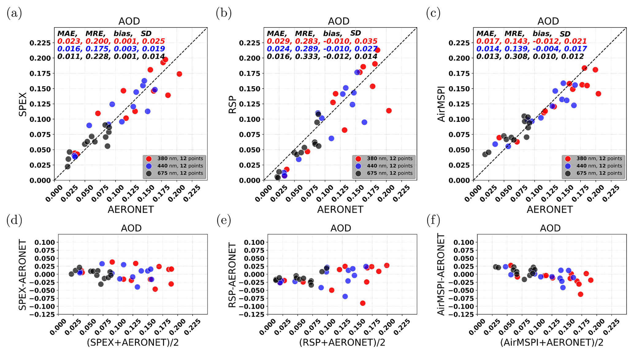
Figure 1Comparison with AERONET for AOD (380, 440, and 675 nm) among SPEX, RSP, and AirMSPI retrievals. (a, b, c) SPEX, RSP, and AirMSPI comparison with AERONET, respectively. (d, e, f) Bland–Altman plots (or difference plots) between SPEX and AERONET, between RSP and AERONET, and between AirMSPI and AERONET, respectively.

Download

For the AOD at 440 nm, the MAE is respectively 0.016, 0.024, and 0.014, the MRE is respectively 0.175, 0.289, and 0.139, the bias is respectively 0.003, −0.010, and −0.004, and the SD is respectively 0.019, 0.027, and 0.017 for SPEX, RSP, and AirMSPI. The MAE, bias, and SD are within 0.01 and the MRE is within 0.15 for the instruments, whereas the values for SPEX airborne and AirMSPI are somewhat smaller than for RSP. Similar conclusions hold for the AOD at 380 or 675 nm. For each instrument, the MAE gets smaller with increasing wavelengths, which is mainly caused by the fact that the AOD value itself decreases with wavelength. Based on the comparisons above, we can conclude that SPEX, RSP, and AirMSPI all achieve good agreement with AERONET and the differences in performance between the instruments are small.

For the comparison of the fine- and coarse-mode effective radius ($r_{\mathrm{eff}}^{\mathrm{f}}$ and $r_{\mathrm{eff}}^{\mathrm{c}}$), it should be noted that it is difficult to retrieve them when AOD is small. Therefore, shown in Fig. 2 is the comparison when τ₃₈₀ is larger than 0.1. The remaining cases are still very challenging but we would lose too many points if we further increase the AOD limit. The solid lines shown in the plot are bias±SD. The retrievals of $r_{\mathrm{eff}}^{\mathrm{f}}$ compared with AERONET are shown in Fig. 2a–c, where the MAE is 0.022, 0.021, and 0.028 µm for SPEX, RSP, and AirMSPI, respectively. SPEX and RSP compare somewhat better in terms of MAE and bias, whereas AirMSPI has a small SD. However, overall the differences between the instruments are small and the number of comparison points is very limited, which means that differences between instruments can be explained by one or two points. The $r_{\mathrm{eff}}^{\mathrm{c}}$ comparisons corresponding to SPEX, RSP, and AirMSPI are shown in Fig. 2d–f, respectively. All three instruments have a poor comparison with AERONET for $r_{\mathrm{eff}}^{\mathrm{c}}$, with an MAE close to 1.5 µm. This is in line with synthetic studies (e.g., Hasekamp et al., 2019a) showing that $r_{\mathrm{eff}}^{\mathrm{c}}$ is a difficult parameter to retrieve, in particular for small AOD values. It should be noted that AERONET consistently gives a larger coarse-mode effective radius than MAPs. A possible explanation is that the effective radius for the coarse modes 4 and 5 in our five-mode retrieval is 0.882 and 1.719, respectively (see Table 1); thus, the coarse-mode effective radius from MAPs calculated based on Eq. (8) is estimated and limited between 0.882 and 1.719, whereas AERONET gives values between 2.25 and 3.3 (when τ₃₈₀ is larger than 0.1). A comparable range is expected for MAPs if a parametric two-mode retrieval or a seven-mode retrieval (Fu and Hasekamp, 2018) is used. Also, it should be noted that “fine” and “coarse” as defined by the almucantar retrievals are different than defining fine and coarse by specific modes as shown in Table 1. This may introduce differences in the comparisons.

Figure 2Comparison with AERONET for the effective radius of the fine and coarse modes ($r_{\mathrm{eff}}^{\mathrm{f}}$ and $r_{\mathrm{eff}}^{\mathrm{c}}$) among SPEX, RSP, and AirMSPI retrievals. (a, b, c) Bland–Altman plots for $r_{\mathrm{eff}}^{\mathrm{f}}$ between SPEX and AERONET, between RSP and AERONET, and between AirMSPI and AERONET, respectively. (d, e, f) Bland–Altman plots for $r_{\mathrm{eff}}^{\mathrm{c}}$ between SPEX and AERONET, between RSP and AERONET, and between AirMSPI and AERONET, respectively.

Download

For the comparison of the fine- and coarse-mode AOD (τ^f and τ^c), the results are shown in Fig. 3. The comparison shows an MAE of 0.028, 0.029, and 0.012 for SPEX, RSP, and AirMSPI, respectively, for τ^f and 0.026, 0.028, and 0.017 for τ^c. The bias is 0.028, 0.019, and 0.004 for τ^f and 0.025, 0.028, and 0.003 for τ^c. So, SPEX and RSP have an overestimation of the fine mode and an underestimation of the coarse mode compared to the AERONET SDA product. Although these biases are large in a relative sense (given the low AOD, especially for the coarse mode), they are within the expected error from the AERONET SDA product. AirMSPI compares better to the AERONET SDA product than SPEX airborne and RSP. Again, it should be noted that the AirMSPI comparison does not contain exactly the same points as the comparison for SPEX and RSP. It should also be noted that for RSP, since no SWIR channels are included in the retrieval to nail the coarse mode, we do not expect it to do well in retrieving coarse-mode properties. It is important to note that for the low AOD values encountered during ACEPOL, the AERONET-retrieved fine- and coarse-mode AOD and effective radius are very uncertain themselves. Therefore, this comparison should not be interpreted as “retrieval versus truth” but rather as “retrieval versus retrieval”.

Figure 3Comparison with AERONET for the AOD of the fine and coarse modes (${\mathit{\tau }}_{\mathrm{500}}^{\mathrm{f}}$ and ${\mathit{\tau }}_{\mathrm{500}}^{\mathrm{c}}$) among SPEX, RSP, and AirMSPI retrievals. (a, b, c) Bland–Altman plots for ${\mathit{\tau }}_{\mathrm{500}}^{\mathrm{f}}$ between SPEX and AERONET, between RSP and AERONET, and between AirMSPI and AERONET, respectively. (d, e, f) Bland–Altman plots for ${\mathit{\tau }}_{\mathrm{500}}^{\mathrm{c}}$ between SPEX and AERONET, between RSP and AERONET, and between AirMSPI and AERONET, respectively.

Download

4.2 Comparison between SPEX airborne, RSP, and HSRL-2

For the comparison to HSRL-2, we only use SPEX airborne and RSP because these provided a continuous data stream during ACEPOL, while AirMSPI only provides step-and-stare measurements for specific targets.

4.2.1 Comparison HSRL-2 to AERONET

Given that we use HSRL-2 as a reference for our MAP retrievals, it is important to first validate HSRL-2 with AERONET. Figure 4 shows the comparison of the HSRL-2 AOD at 355 and 532 nm with AERONET (log–log interpolated between 340 and 380 nm for 355 nm and between 500 and 675 nm for 532 nm). From the comparison it follows that the HSRL-2 AOD at 532 nm agrees very well with AERONET, with a small MAE (0.012), a small MRE (0.269), a small absolute bias (0.005), and a small SD (0.014). The comparison at 355 nm is somewhat worse than that at 532 nm with an MAE of 0.028, an MRE of 0.357, a bias of −0.014, and an SD of 0.029. The bias between HSRL-2 and AERONET is within the AERONET uncertainty. The random differences, with standard deviation 0.029 at 380 nm and 0.014 at 532 nm, are most likely due to HSRL-2 uncertainties. Note that shown in Fig. 4 are the points corresponding to the days 23 October, 25 October, 26 October, and 7 November 2017.

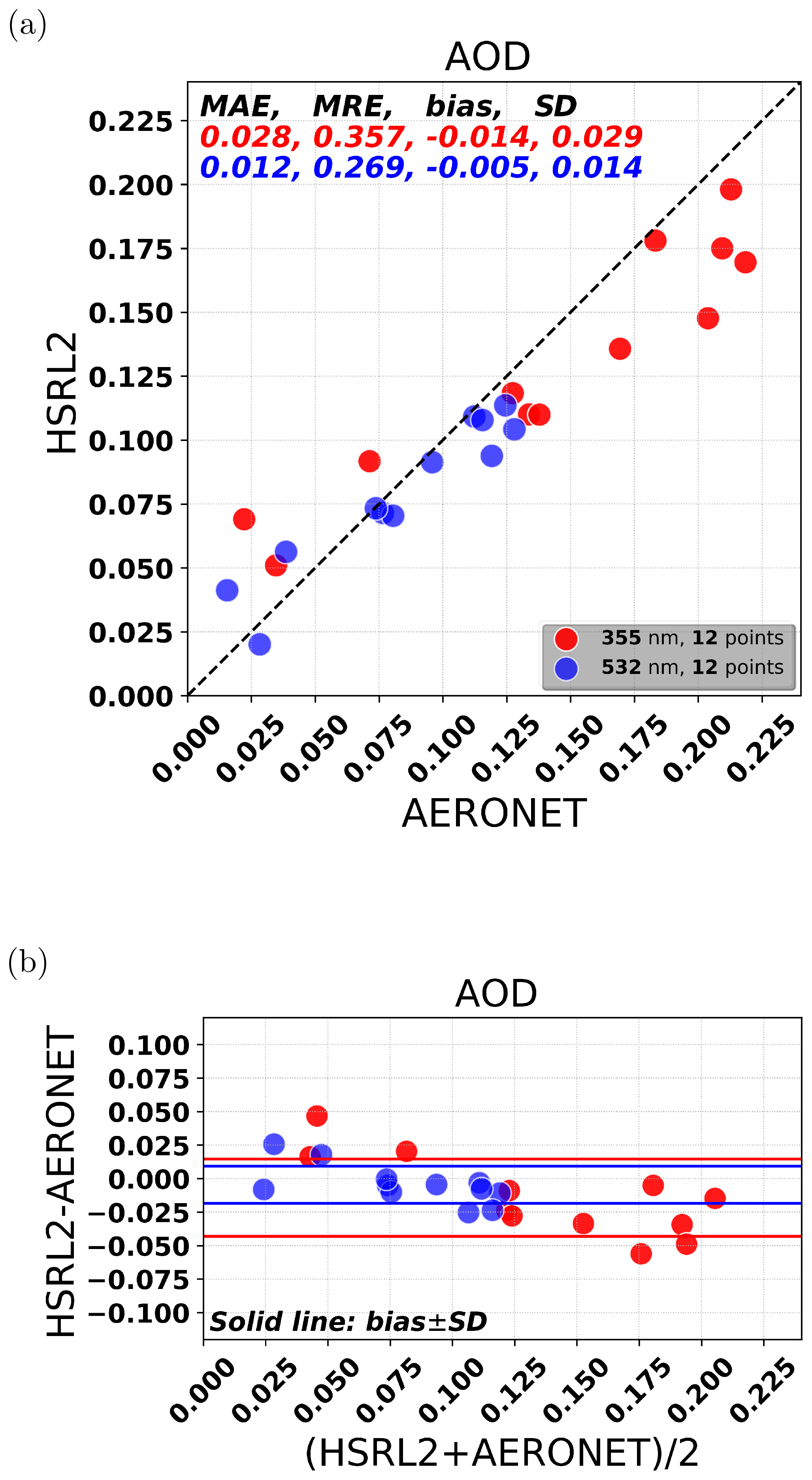
Figure 4Comparison between HSRL-2 and AERONET for AOD at 355 and 532 nm. (a, b) The scatter plot and the difference plot, respectively.

Download

4.2.2 Low AOD case on 26 October 2017

In this subsection, we compare the aerosol properties from SPEX and RSP with those from HSRL-2 for 26 October 2017 with low aerosol loading (AOD at 532 nm in the range 0.02 to 0.14). The results for AOD at 355 and 532 nm are shown in Fig. 5. Figure 5a shows the retrieved AOD from HSRL-2 for the ground pixels colocated with SPEX and RSP. From this figure it follows that there were very low AOD values for the eastern part of the scene and somewhat higher values in the western and southwestern part of the scene. Figure 5b shows the AOD comparison between SPEX and HSRL-2 with the MAE 0.014, the MRE 0.296, the bias 0.009, and the SD 0.018 at 532 nm, as well as the MAE 0.028, the MRE 0.321, the bias −0.006, and the SD 0.034 at 355 nm. Figure 5c shows the AOD comparison between RSP and HSRL-2 with the MAE 0.022, the MRE 0.418, the bias −0.007, and the SD 0.028 at 532 nm, as well as the MAE 0.037, the MRE 0.369, the bias −0.008, and the SD 0.048 at 355 nm. So, SPEX shows a very good agreement with HSRL-2 for this challenging scene of low AOD over land with a relatively bright surface. SPEX compares somewhat better to HSRL-2 than RSP for this case at both 532 and 355 nm. The Bland–Altman plots Fig. 5e and f show a larger scatter and more outliers for RSP. A possible explanation is that for low AOD the radiance and polarization measurements have a strong influence from the spatially inhomogeneous surface, and therefore errors due to inter-angle misregistration, which are larger for RSP than for SPEX, may be significant. For these cases there is larger sensitivity to spatial mismatch between different viewing angles, and RSP, as a single-pixel-swath instrument, is more sensitive to such mismatches. Figure 5d shows the AOD comparison between SPEX and RSP with the MAE 0.024, the MRE 0.831, the bias 0.016, and the SD 0.025. The differences from the direct comparison between SPEX and RSP are somewhat larger than those from individual comparisons of HSRL-2 with SPEX and RSP. This suggests that the differences with HSRL-2 are not caused by common assumptions in the SPEX and RSP retrievals but are rather caused by errors that are specific to each MAP.

Figure 5Comparison with HSRL-2 from 26 October 2017 (low AOD case) for AOD (355 and 532 nm) between SPEX and RSP retrievals. (a) HSRL-2 AOD colocation with SPEX and RSP. (The map is generated using Python's basemap package and its ArcGIS image service ESRI_Imagery_World_2D.) (b) SPEX AOD comparison with HSRL-2. (c) RSP AOD comparison with HSRL-2. (d) SPEX AOD comparison with RSP. (e, f, g) Bland–Altman plots for (b, c, d), respectively.

For the retrieved surface parameters, we do not have a good reference to evaluate the accuracy. Instead, Fig. 6 shows the AOD difference between MAP and HSRL-2 as a function of the retrieved BRDF scaling parameter A, for which we do not see clear correlation or dependence.

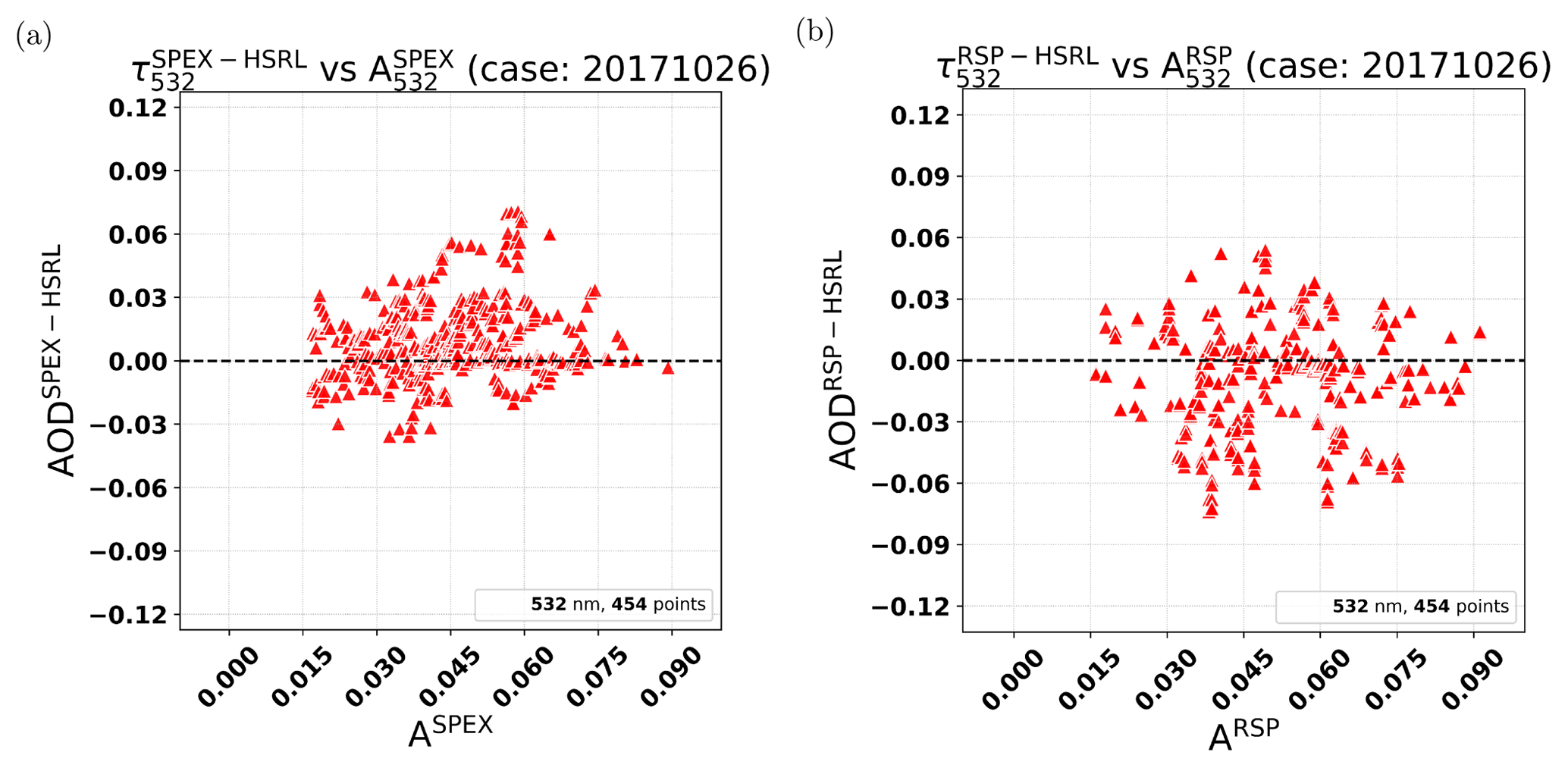
Figure 6The AOD difference between MAP and HSRL-2 as a function of the retrieved BRDF scaling parameter A at 532 nm. (a) AOD difference between SPEX and HSRL-2 versus A. (b) AOD difference between RSP and HSRL-2 versus A.

Download

4.2.3 High AOD on 9 November 2017

In this subsection, polarimetric retrievals from SPEX airborne and RSP are compared to HSRL-2 on 9 November 2017 for a smoke plume with high AOD (including AOD values >1.0). Figure 7a shows the original AOD (i.e., no filter or colocation included) from SPEX for the flight leg over the smoke plume. This gives a sense of how variable the smoke plume is. Figure 7b shows the AOD comparison between SPEX and HSRL-2, for which the MAE is 0.088, the MRE is 0.693, the bias is −0.029, and the SD is 0.149 at 532 nm. Figure 7c shows the AOD comparison between RSP and HSRL-2, for which the MAE is 0.079, the MRE is 0.564, the bias is −0.024, and the SD is 0.142 at 532 nm. Figure 7d shows the AOD comparison between SPEX and RSP, for which the MAE is 0.044, the MRE is 0.155, the bias is −0.005, and the SD is 0.063 at 532 nm. RSP compares slightly better to HSRL-2 than SPEX with respect to MAE and MRE. It should be noted that the smoke plume exhibits large spatial variation, so part of the MAP–lidar differences can be attributed to the fact that different instruments see a slightly different part of the smoke plume. Furthermore, both SPEX and RSP show a similar negative bias in AOD at both 355 and 532 nm, as well as one clear outlier point in the comparison with HSRL-2 at the highest AOD. This is also clear from the corresponding Bland–Altman plots in Fig. 7e and f. Given the very similar underestimation in both SPEX and RSP (compared to HSRL-2) and the good comparison between SPEX and RSP, it is unlikely that this underestimation is caused by aspects related to instrumental errors of the two different MAPs. It might be possible that the underestimation is related to the MAP retrieval approach, which is the same for both instruments, but based on earlier studies with real and synthetic measurements we have no indication for this. Another possibility is that HSRL-2 overestimates the AOD at this high aerosol loading or the large spatial variability has a larger effect on the MAP–lidar comparison than on the inter-MAP comparison. At high AOD the performance of RSP is more similar to that of SPEX than for low AOD. Our explanation for this is that at high AOD the measured radiance and DoLP are less affected by the co-registration errors between viewing angles than for low AOD.

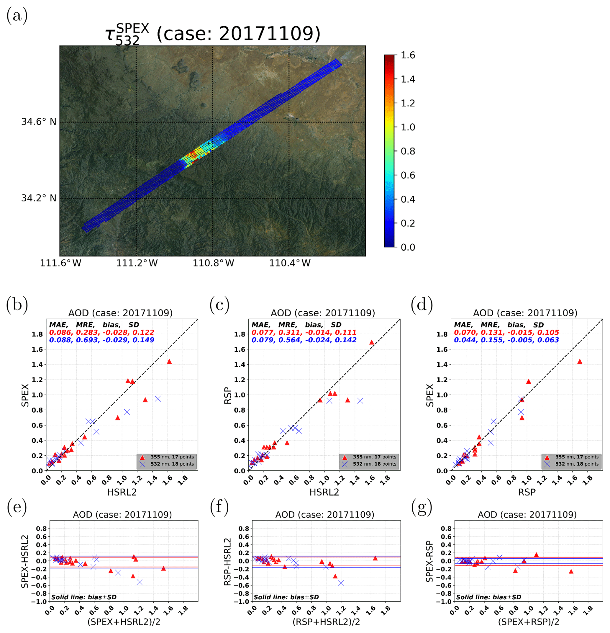
Figure 7Comparison with HSRL-2 from 9 November 2017 (high AOD smoke case) for AOD (355 and 532 nm) between SPEX and RSP retrievals. (a) SPEX original AOD, i.e., no filter or colocation included. (The map is generated using Python's basemap package and its ArcGIS image service ESRI_Imagery_World_2D.) (b) SPEX AOD comparison with HSRL-2. (c) RSP AOD comparison with HSRL-2. (d) SPEX AOD comparison with RSP. (e, f, g) Bland–Altman plots for (b, c, d), respectively.

For the high AOD case, we also compare the aerosol depolarization ratio (δ) and aerosol lidar ratio (S) from SPEX and RSP with HSRL-2. Figure 8a–c respectively show the comparison of the aerosol depolarization ratio between SPEX and HSRL-2, between RSP and HSRL-2, and between SPEX and RSP. It can be observed that both SPEX and RSP show a similar behavior against HSRL-2, especially at 355 nm: there is an underestimation towards lower values of the depolarization ratio, but, on the other hand, there is a reasonable agreement with HSRL-2 for both instruments. Again, given the fact that the performance of both SPEX and RSP versus HSRL-2 is very similar, we conclude that the main reason for the difference between SPEX/RSP and HSRL-2 does not lie in instrumental errors for the MAPs. A possible explanation for the difference could be the simplified description of nonspherical particles in our retrieval approach. On the other hand, the overall comparison of the aerosol depolarization ratio with HSRL-2 confirms the capability of both SPEX and RSP to retrieve information on particle shape. The results of the aerosol lidar ratio are shown in Fig. 8d–f. Both SPEX and RSP show a similar overestimation of the lidar ratio compared to HSRL-2, and SPEX and RSP agree quite well. Again, it is unlikely that the overestimation is related to instrumental errors in the MAPs. Overall, the agreement with HSRL-2 for the aerosol lidar ratio is reasonable for both SPEX and RSP.

4.2.4 Median and standard deviation properties of the smoke plume

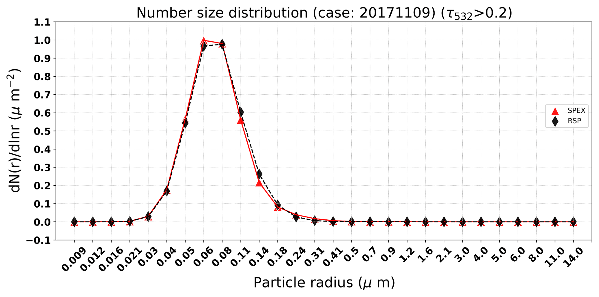
The median and standard deviation properties for the smoke plume as measured by SPEX and RSP are summarized in Table 3. Here, we only include retrievals for which AOD>0.2 at 532 nm because for those cases the accurate retrieval of microphysical properties is expected (e.g., Hasekamp et al., 2019a). The number of points to calculate the median and the standard deviation is the same for SPEX and RSP. Also, we only include fine-mode microphysical properties because there is only a very small coarse-mode contribution to the smoke plume. SPEX and RSP compare well for the fine-mode refractive index, fine-mode effective radius, fine- and coarse-mode AOD, and SSA (relative to requirements as formulated, e.g., by Mishchenko et al., 2004). Reasonable agreement is found for the fraction of spherical particles. For the aerosol layer height (ALH), SPEX retrieves a higher value (4.417 km) than RSP (1.148 km), and the latter value is somewhat closer to the ALH derived from HSRL-2 (2.64 km). Here, it should be noted that for SPEX the shortest wavelength used in the retrieval is 450 nm, so we do not expect an accurate ALH retrieval because the retrieval of ALH from polarization requires a strong signal from Rayleigh scattering (Wu et al., 2016). Figure 9 shows the number particle size distribution from SPEX and RSP in the smoke plume, which confirms that the smoke plume is fine-mode dominated.

Table 3Median and standard deviation (SD) properties of the smoke plume from SPEX and RSP when AOD>0.2 at 532 nm.

Download Print Version | Download XLSX

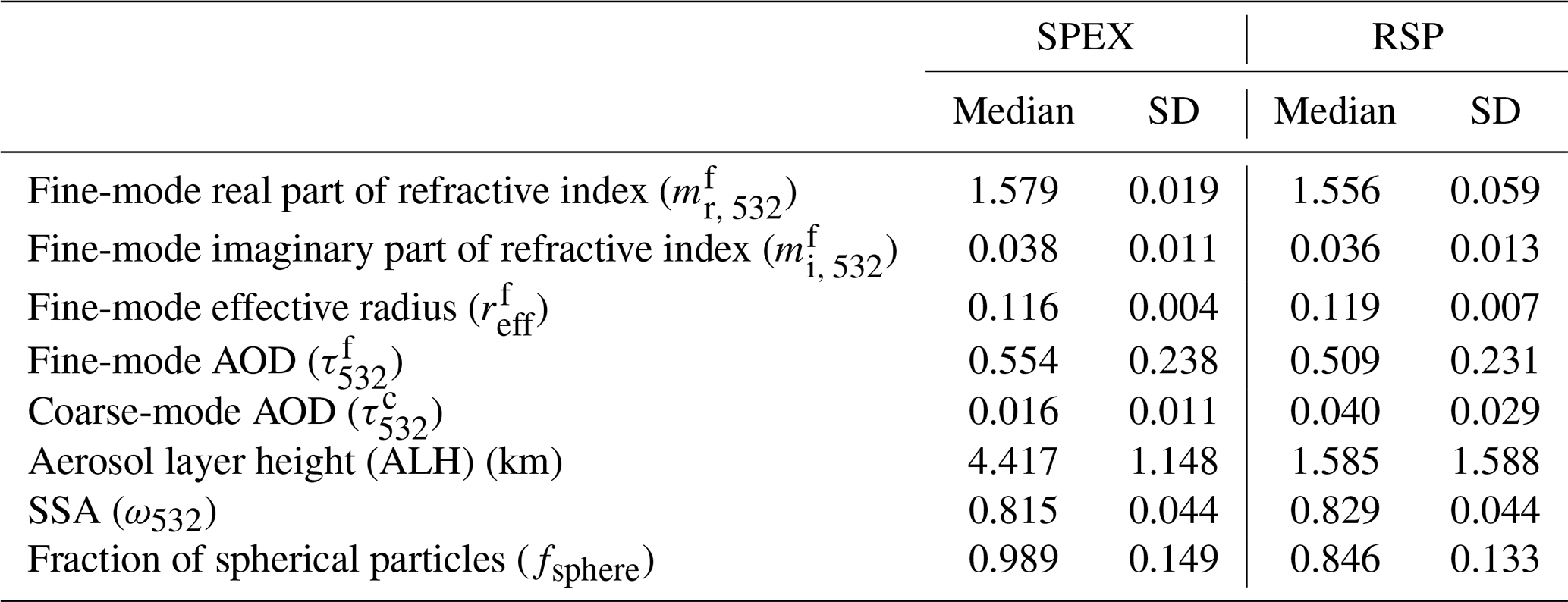
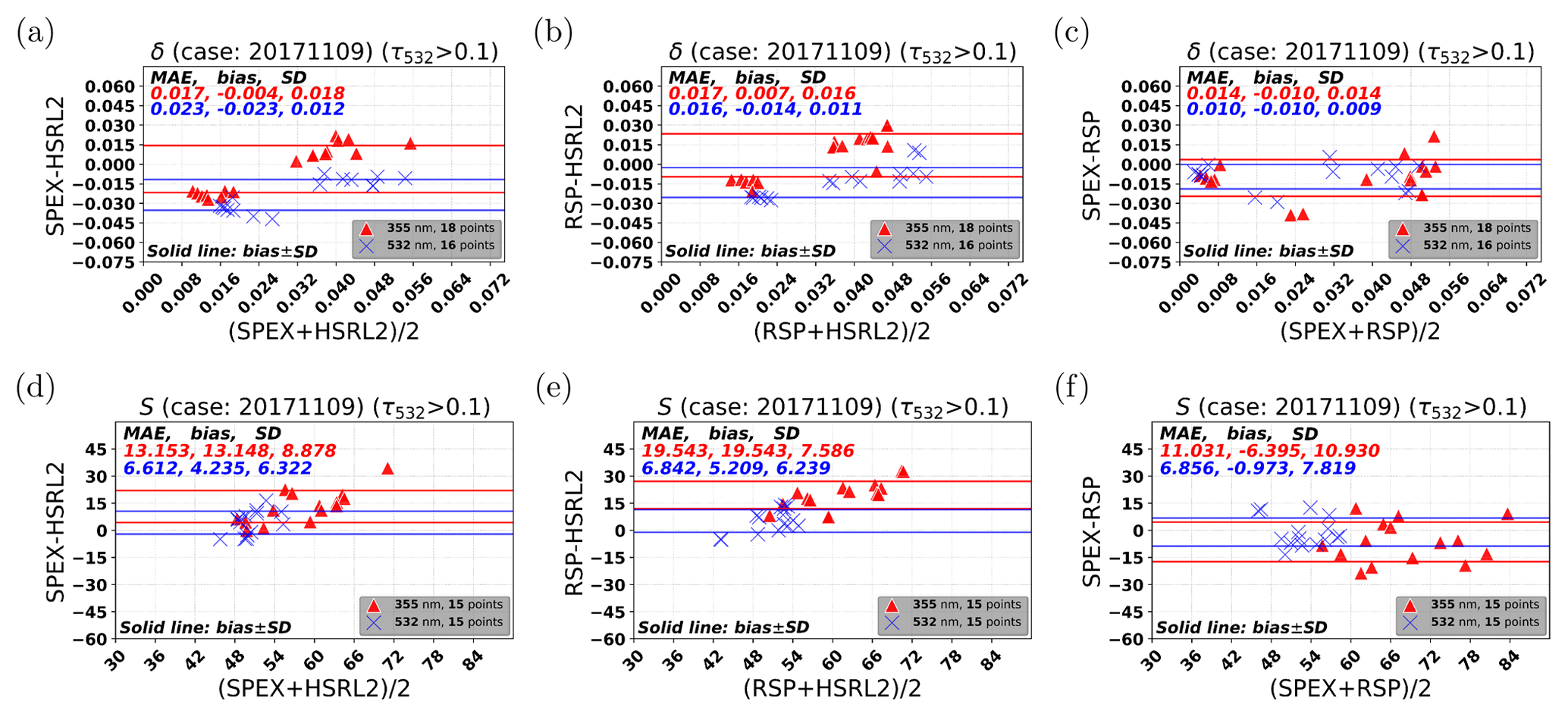
Figure 8Comparison with HSRL-2 from 9 November 2017 (high AOD smoke case) for the aerosol depolarization ratio (δ) and the aerosol lidar ratio (S) between SPEX and RSP retrievals. (a) SPEX δ comparison with HSRL-2. (b) RSP δ comparison with HSRL-2. (c) SPEX δ comparison with RSP. (d) SPEX S comparison with HSRL-2. (e) RSP S comparison with HSRL-2. (f) SPEX S comparison with RSP.

Download

Figure 9Number particle size distribution in the smoke plume retrieved from SPEX and RSP.

Download

The values of the aerosol properties in Table 3 (for both SPEX and RSP) are in the range that is expected for smoke. First of all, it is expected that smoke is dominated by fine particles (e.g., Russell et al., 2014), which is confirmed by the much larger retrieved fine-mode AOD than coarse-mode AOD by both MAPs. The real part of the refractive index is consistent with the study of Levin et al. (2010) for the Fire Laboratory at Missoula Experiment (FLAME), who found mostly refractive indices for biomass burning between 1.55 and 1.60. Also, the SSA values in Table 3 are representative for fresh biomass burning smoke. For example, Nicolae et al. (2013) found SSA values of 0.79 at 532 nm for smoke with an age of 0.25 d and 0.93 for smoke with an age of 0.75 d. Both the values retrieved by SPEX and RSP can be considered realistic for smoke.