the Creative Commons Attribution 4.0 License.
the Creative Commons Attribution 4.0 License.
 | 13 Feb 2020
Evaluating different methods for elevation calibration of MAX-DOAS (Multi AXis Differential Optical Absorption Spectroscopy) instruments during the CINDI-2 campaign
Sebastian Donner
Jonas Kuhn
Michel Van Roozendael
Alkiviadis Bais
Steffen Beirle
Tim Bösch
Kristof Bognar
Ilya Bruchkouski
Ka Lok Chan
Steffen Dörner
Theano Drosoglou
Caroline Fayt
Udo Frieß
François Hendrick
Christian Hermans
Junli Jin
Ang Li
Jianzhong Ma
Enno Peters
Gaia Pinardi
Andreas Richter
Stefan F. Schreier
André Seyler
Kimberly Strong
Jan-Lukas Tirpitz
Yang Wang
Pinhua Xie
Jin Xu
Xiaoyi Zhao
Thomas Wagner
We present different methods for in-field elevation calibration of MAX-DOAS (Multi AXis Differential Optical Absorption Spectroscopy) instruments that were applied and inter-compared during the second Cabauw Intercomparison campaign for Nitrogen Dioxide measuring Instruments (CINDI-2). One necessary prerequisite of consistent MAX-DOAS retrievals is a precise and accurate calibration of the elevation angles of the different measuring systems. Therefore, different methods for this calibration were applied to several instruments during the campaign, and the results were inter-compared.
This work first introduces and explains the different methods, namely far- and near-lamp measurements, white-stripe scans, horizon scans and sun scans, using data and results for only one (mainly the Max Planck Institute for Chemistry) instrument. In the second part, the far-lamp measurements and the horizon scans are examined for all participating groups. Here, the results for both methods are first inter-compared for the different instruments; secondly, the two methods are compared amongst each other.
All methods turned out to be well-suited for the calibration of the elevation angles of MAX-DOAS systems, with each of them having individual advantages and drawbacks. Considering the results of this study, the systematic uncertainties of the methods can be estimated as for the far-lamp measurements and the sun scans, for the horizon scans, and around for the white-stripe and near-lamp measurements. When comparing the results of far-lamp and horizon-scan measurements, a spread of around 0.9∘ in the elevation calibrations is found between the participating instruments for both methods. This spread is of the order of a typical field of view (FOV) of a MAX-DOAS instrument and therefore affecting the retrieval results. Further, consistent (wavelength dependent) offsets of 0.32∘ and 0.40∘ between far-lamp measurements and horizon scans are found, which can be explained by the fact that, despite the flat topography around the measurement site, obstacles such as trees might mark the visible horizon during daytime. The observed wavelength dependence can be explained by surface albedo effects. Lastly, the results are discussed and recommendations for future campaigns are given.
- Article
(9592 KB) - Full-text XML
- BibTeX
- EndNote


Multi AXis Differential Optical Absorption Spectroscopy (MAX-DOAS) is a well established method of ground-based remote sensing of trace gases and aerosols. MAX-DOAS instruments measure spectra of scattered sunlight at different (mostly low) elevation angles. Therefore, they have a high sensitivity to trace gases and aerosols located close to the surface (e.g. Hönninger and Platt, 2002; Hönninger et al., 2004; Irie et al., 2008; Van Roozendael et al., 2004; Wagner et al., 2004, 2011; Wittrock et al., 2004). Such measurements allow for the retrieval of vertical profiles of trace gases and aerosol extinction as well as column properties such as vertical column densities (VCDs) and aerosol optical depths (AODs) (e.g. Frieß et al., 2006; Irie et al., 2008; Clémer et al., 2010; Wagner et al., 2011).
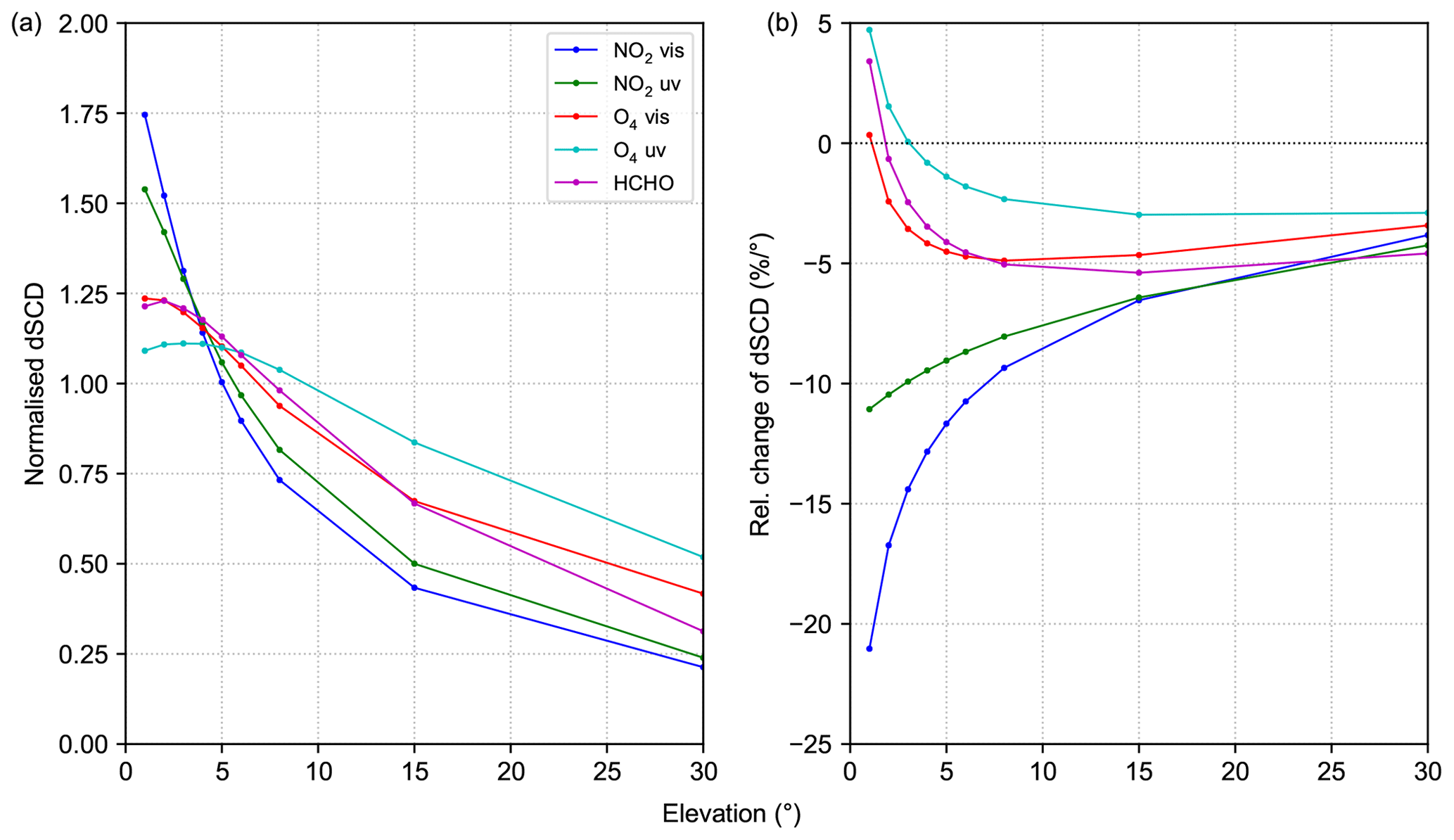
Figure 1(a) Mean dependence of the trace-gas dSCDs on the elevation angle for the whole campaign. Each curve was normalised to the mean dSCD value of the elevation sequence. (b) Relative change of the measured dSCDs per degree pointing error at different elevation angles.
For the retrieval of these quantities, it is crucial to accurately know the measurement geometry, namely the solar zenith angle, the relative solar azimuth angle and the telescope's elevation angle (Hönninger et al., 2004). While the solar zenith angle can be computed rather easily, it is more difficult to determine the relative solar azimuth angle and to calibrate the telescope's elevation angles. Although the relative azimuth has at least the same uncertainties as the elevation angle, it has a much weaker effect on the measurements (when assuming horizontal homogeneity of the trace-gas distributions). An analysis of the CINDI-2 data set shows that, for low elevation angles, wrong pointing has a large impact on the retrieved trace-gas differential slant column densities (dSCDs), which are the basic quantity obtained by MAX-DOAS (Hönninger et al., 2004). Fig. 1a shows the mean dependence of the dSCDs on the elevation angle for the whole campaign and for different trace gases. Each curve was normalised to the mean dSCD of the respective elevation sequence. Fig. 1b shows the relative changes in the retrieved trace-gas dSCDs per degree pointing error for the same species. The curves were obtained by calculating the derivative of the dSCD curves from panel (a) with respect to the elevation angle and dividing the results by the dSCDs at the corresponding elevations. Although this approach remains qualitative, it shows clearly under which conditions pointing errors can lead to substantial biases in the dSCDs. As an example, an error of 1∘ in the telescope's elevation close to 0∘ elevation can lead to an error of around 20 % in the retrieved NO2 dSCD, since the sensitivity of MAX-DOAS measurements depends strongly on the elevation angle and NO2 is mainly located close to the surface.
Since instruments and retrieval algorithms have improved significantly in recent years, uncertainties in the elevation calibration now have a larger relative impact on the retrieval results and can become the dominating error source. Therefore, the calibration of the elevation angles of MAX-DOAS instruments has become an important topic for instrument operators (e.g. Roscoe et al., 2010; Piters et al., 2012). In principle, these calibrations can be best done in the laboratory under stable and controlled conditions, where fixed target points are used as references and the corresponding elevations can be calibrated accordingly. In particular, the field of view (FOV) should be determined already in the laboratory. Nevertheless, elevation calibration in the field is indispensable, because, during transport from the laboratory to the field and during installation on the measurement site, it is likely that the instrument characteristics might change. In the past, however, when the instruments were brought to the field, the accuracy of the a priori elevation angle calibration was only rarely (if at all) checked under real measurement conditions.
In this work, different methods for in-field elevation calibration of MAX-DOAS instruments, which were applied by numerous groups during the CINDI-2 campaign, are presented, evaluated and compared amongst each other. Furthermore, recommendations for the setup of MAX-DOAS measurements are derived based on the results of the comparison. This work focuses on the details of the elevation calibration procedure. An assessment of the instrument performance is given in Kreher et al. (2019).
The paper is structured as follows. First, a short overview of the CINDI-2 campaign and the participating instruments is given in Sect. 2. Section 3 introduces and examines the different methods of elevation calibration for one (mainly the instrument of the Max Planck Institute for Chemistry; MPIC) instrument and a first comparison between the different methods is given. Comparisons between the participating instruments for the different methods are presented in Sect. 4. Additionally, the methods are compared amongst each other in detail and an assessment of the in-field FOV determination is presented. A final discussion is presented in Sect. 5, together with conclusions and recommendations for upcoming MAX-DOAS measurements.
2.1 The CINDI-2 campaign
The second Cabauw Intercomparison campaign for Nitrogen Dioxide measuring Instruments (CINDI-2) took place in September 2016 at the Cabauw Experimental Site for Atmospheric Research (CESAR) in the Netherlands. It was a follow-up to the CINDI campaign, which took place at the same site in June 2009 (Roscoe et al., 2010; Piters et al., 2012; Pinardi et al., 2013; Frieß et al., 2016). The main objective of the CINDI-2 campaign was the intercomparison of different ground-based remote sensing – mostly MAX-DOAS – instruments, including several calibration exercises to harmonise the measurements of the different instruments. For the interpretation of the trace-gas (e.g. NO2) intercomparisons, an accurate and consistent elevation calibration is essential. Therefore, an elevation calibration exercise was included in the campaign plan. More detailed descriptions of the CINDI-2 campaign and its objectives are given in Kreher et al. (2019) and Apituley et al. (2020).
Drosoglou et al. (2017)Clémer et al. (2010)Schreier et al. (2019)Bruchkouski et al. (2014)Peters et al. (2012)Lampel et al. (2015)Lampel et al. (2015)Donner (2016)Fraser et al. (2009)Table 1Overview of the key properties of the instruments participating in the elevation calibration exercise. The table lists the institute names, the corresponding instrument names and their acronyms (columns 1–3). Further, the instrument types (1-D or 2-D) as well as the spectral range and resolution for each instrument are summarised in columns 4 to 6. Additionally, the number of detectors and light couplings, the type of light coupling (fibre F or direct D), and the instrument fields of view (FOV) are specified (columns 7–9). Finally, the corresponding detector temperatures and references explaining the individual instruments in more detail are given (columns 10 and 11).
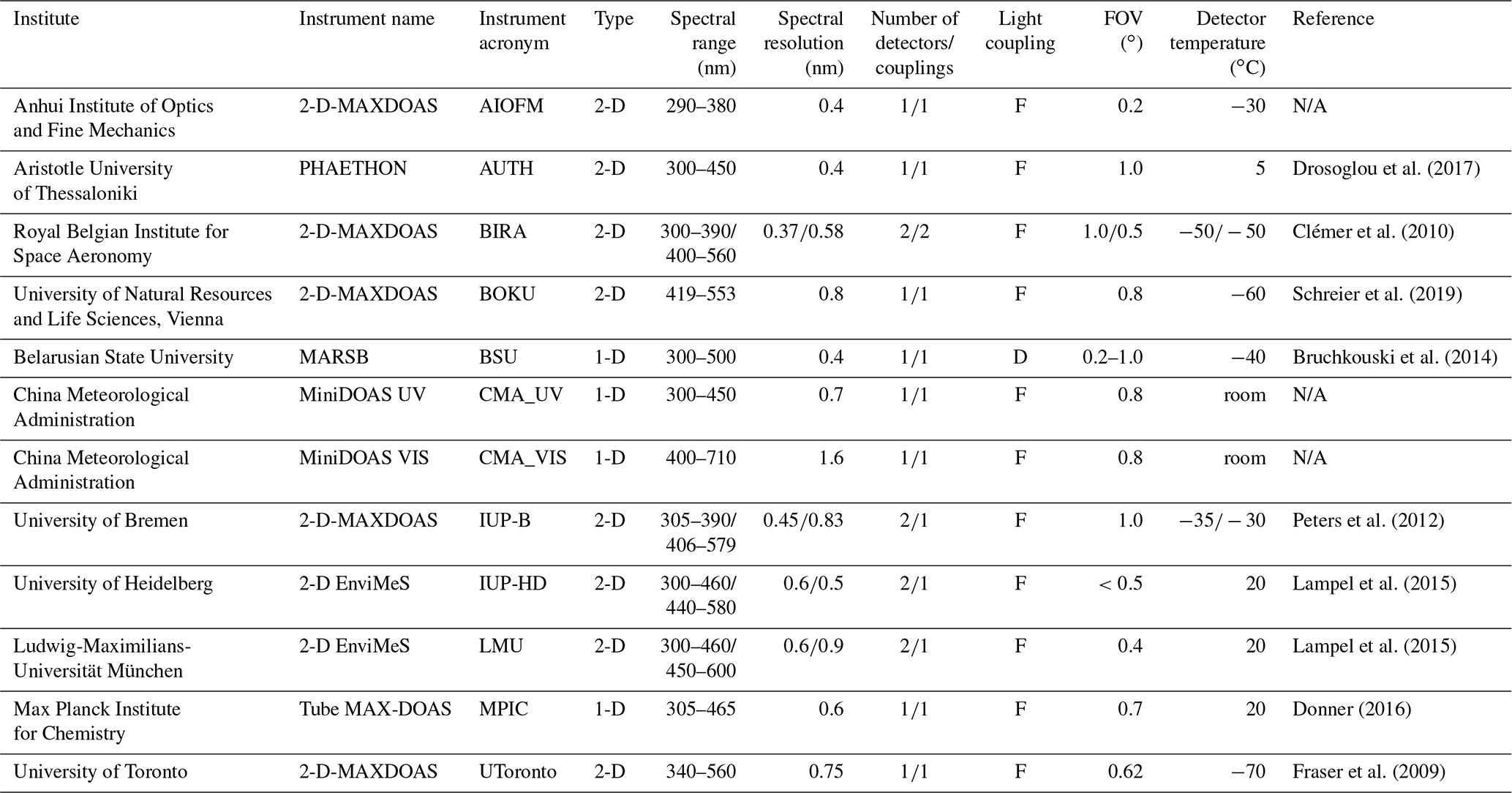
N/A indicates instruments for which no specific references are available.
Many instruments which were operated during the campaign also participated in different elevation calibration exercises that were conducted throughout CINDI-2 and are summarised in this work. In the following subsection, some technical details of the different instruments are presented.
2.2 Participating MAX-DOAS instruments
Several instruments from various groups participated in the elevation calibration exercise. Since horizon scans were part of the standardised measurement protocol (Kreher et al., 2019; Apituley et al., 2020), they were performed by in total 28 instruments. However, only 12 instruments from 11 groups participated actively in the other calibration exercise, namely the far-lamp measurements. Therefore, only these are included in Table 1, which provides an overview on the key properties of the instruments which are of relevance for this study. Further, this table defines instrument acronyms and names. Table 1 is based on the CINDI-2 planning document and information given in Kreher et al. (2019), where additional details on the instruments are provided. Finally, this table indicates the variety and different properties of the participating instruments.
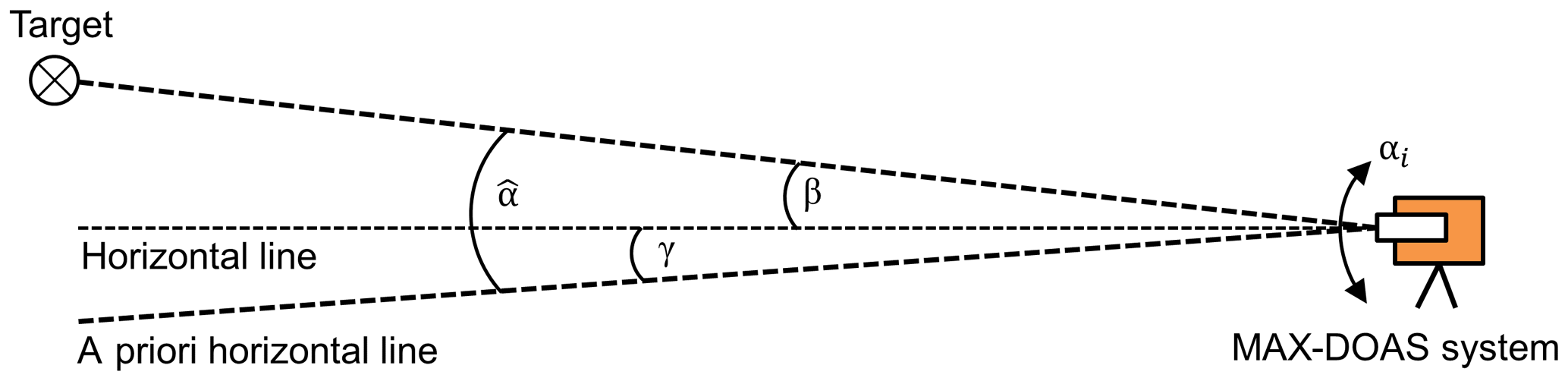
Figure 2Sketch of the general experimental setup and angle definition used in this study. The horizontal line corresponds to the line of sight of the instrument at 0∘ elevation.
This section introduces the different methods for the calibration of the elevation angles of MAX-DOAS instruments that were applied by at least one group during the CINDI-2 campaign. First, the common general approach which is underlying all methods is explained (Sect. 3.1), followed by detailed descriptions and evaluations of the individual methods (Sect. 3.2 to 3.6). Section 3.7 gives a consistency check between the different methods using data of the MPIC instrument.
3.1 General approach
As already mentioned, MAX-DOAS instruments which are brought to field campaigns typically have an a priori calibration of the elevation angles, which was obtained in the laboratory. Different procedures of laboratory elevation calibrations were used by the groups participating in this study. A large fraction of the groups verified the alignment of the telescope and the optical system through retro-illumination of the quartz fibre bundle and measurement of the position of the resulting light spot on a wall, where target points were located. Others used high-precision water levels to check this alignment or even performed no laboratory elevation calibrations. The groups reported that the accuracies and precisions of these procedures are in a range from roughly 0.1∘ to 1∘. However, all this might be overruled by uncertainties introduced during transport or on the measurement site (tripod movements, building movements, imperfect horizontal alignment of telescope head on tripod, etc.). For high-quality measurements, this a priori calibration has to be checked and (if needed) to be adjusted in field. If the optical axis would be precisely known, a water level would be completely sufficient to calibrate the elevation angles. But this assumption is not always fulfilled, e.g. because the fibre bundle is not perfectly centred. For those reasons, five different methods for the in-field calibration of the elevation angles of MAX-DOAS systems are described and evaluated in the following sections. All of them use the same basic principle, which is described in this section.
First, a specific target is placed in front of the optical unit of a MAX-DOAS instrument (see Fig. 2). The elevation angle β of this target relative to the horizontal line of the telescope unit has to be determined very accurately in order to use this elevation as a reference. Next, an elevation scan across the target is performed and the apparent elevation angle of the target is retrieved using the measured intensities at different elevation angles αi. Here, αi denotes elevation angles measured relative to the a priori elevation calibration of the instrument. In that way, an elevation offset can be calculated and used to correct the elevation angles measured relative to the a priori elevation calibration of the instrument (). Further, this offset γ can be used to adjust the a priori elevation calibration of the MAX-DOAS system by shifting the a priori horizontal line by −γ. It should be noted that this principle used by all the different methods described in this work only calibrates one specific elevation angle (usually 0∘). Thus, the accuracy of the other elevations depends on the internal accuracy of the motor and its steering unit. Many instruments (e.g. the CMA MiniDOAS instrument and the MPIC Tube MAX-DOAS instrument) approach the other elevation angles by moving the telescope by a defined number of motor steps (per degree) relative to the motor position that corresponds to the horizontal line of the telescope (0∘ elevation). Others (e.g. the 2-D EnviMeS instruments) use an inclinometer inside the telescope unit, which also enables these instruments to actively correct their elevation angles for possible deviations. According to the instrument's manufacturer, the accuracy of the inclinometers used for the EnviMeS instruments is 0.1∘ and the precision is 0.03∘. Many other methods to deal with this internal elevation calibration are possible, but this topic is not discussed in more detail in this paper. Further, it should be mentioned that the elevation calibration might be different for different azimuthal directions, which is important for 2-D instruments.

Figure 3Upper panel: map indicating the position of both the lamp and the MAX-DOAS instruments. Lower panel: sketch of the setup for the far-lamp measurements during the CINDI-2 campaign. Note that the lamp is placed below the height of the telescope, and therefore a slightly negative elevation of is expected (see text).
A sketch of the general measurement setup can be found in Fig. 2; further, a graphic definition of all relevant angles is provided in this figure. In the following sections this principle is applied to different target types and the results are evaluated.
3.2 Far-lamp measurements
3.2.1 Approach
For the first method, an artificial light source is used as target that is located at a far distance (around 1 to 2 km) from the instrument's telescope and typically close to the visible horizon. Since this method uses an artificial light source, the elevation scan across this target has to be done during nighttime.
During the CINDI-2 campaign, a xenon lamp was used as light source, and it was placed at around 1280 m distance from the measurement site in the main viewing direction of the MAX-DOAS instruments at an azimuth angle of 287∘ (upper panel of Fig. 3). The lamp was put in the focal point of a large-aperture lens with a diameter of 17 cm, which was achieved by minimising the size of the light beam (this was already done prior to the campaign). Then the lamp was manually directed towards the campaign site. Here, it should be noted that the exact pointing is not critical as long as the instruments are located within the light cone. It was assumed that the diameter of the lens is homogeneously bright. Also, this assumption is not a critical point, because the angle under which the full lens is seen from the campaign site is smaller than 0.01∘.
Using the connected water channels located next to both the measurement site and the lamp site, we could determine and mark the vertical position of the lamp at the measurement site (lamp mark in the lower panel of Fig. 3). Therefore, the light of a laser level was projected onto a folding rule which was placed in the nearby channels. In that way, first the height difference between lamp and the channel's water surface could be determined. Since all channels were connected to each other (except one step which was determined in the same way), the lamp position could be marked on the containers as indicated in the lower panel of Fig. 3. Thus, the height difference Δh between the optical units of the instruments and the lamp mark could be determined. This Δh was then used to infer the expected elevation angles β of the lamp relative to the horizontal lines of the optical units of the individual MAX-DOAS systems. The layout of the measurement conditions and the measurement geometry are summarised in Fig. 3.
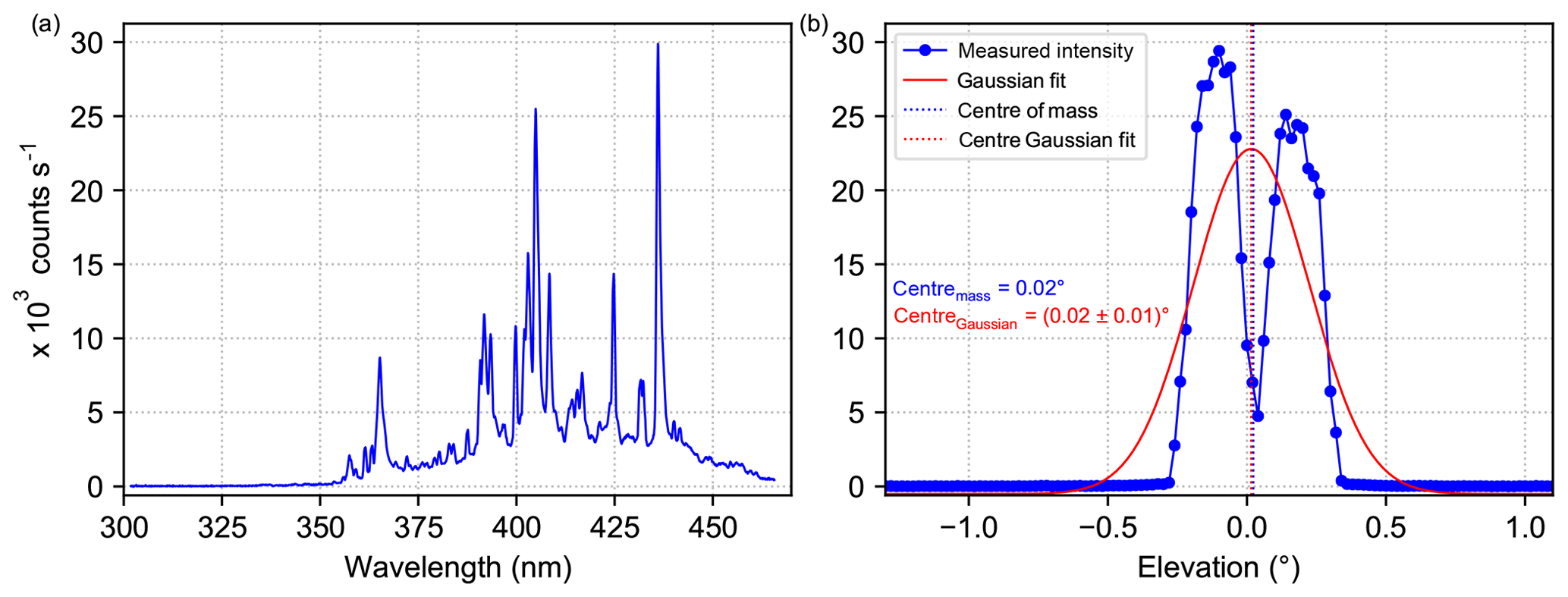
Figure 4(a) Xenon lamp spectrum recorded on 13 September 2016 by the MPIC instrument. The three distinct emission lines at 365.16, 404.90 and 435.96 nm, which are used for the analysis, are clearly visible. (b) Intensity curve at 435.96 nm (blue solid line) recorded on 13 September by the MPIC instrument. The obtained centre of mass is indicated by the dashed blue line. Further, the centre obtained by a Gaussian fit and the corresponding fit are displayed in red.
Such xenon lamp measurements were done on several days (8, 10, 13 and 19 September) throughout the campaign, although not all instruments participated on all nights. In the next section, the analysis of the lamp measurements is explained in more detail using data from the MPIC instrument.
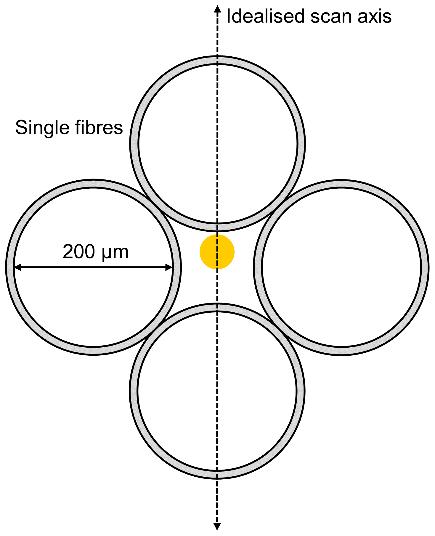
Figure 5Sketch of the fibre bundle placed in the focal point of the telescope of the MPIC instrument. The grey parts indicate the gladding (additional 20 µm) of the fibres. The white circles represent the light-conducting part of the single glass fibres with a diameter of 200 µm, while the yellow spot indicates the idealised image (neglecting aberration and other effects) of the xenon lamp inside the telescope, which has a diameter of 7 µm. Note that the size of the yellow dot is not shown at the correct scale relative to the fibre diameter and is larger than in reality.
3.2.2 Results for the MPIC instrument
Data from the far-lamp measurements are available for four nights for the MPIC instrument. On all of these nights, a fixed elevation calibration (same 0∘ motor position) was used and the scan resolution was 0.02∘ (except on 8 September, when the scan resolution was 0.1∘ as indicated in the last column of Table 2). For the MPIC instrument, the pre-calibration of the elevations was done using a water level during the setup of the instrument. Then finer adjustments were performed using the results of the far-lamp scans from 7 (in this night the lamp measurements were tested by our group with a scan resolution of 0.1∘ but the scanning was done manually), 8 and 10 September. All elevations of the MPIC instrument in this paper are given relative to the elevation calibration, which was obtained by these finer adjustments and which was finally used for the regular measurements.
In the following, the analysis is done for three wavelengths, which are distributed over the detector range of the instrument and correspond to strong emission lines of the xenon lamp. An example spectrum of the xenon lamp which was measured on 13 September is shown in Fig. 4a. The three distinct emission lines at 365.16, 404.90 and 435.96 nm that were used for the analysis are clearly visible.
As first step of the analysis, the measured intensities are normalised with respect to their total integration time and linearly interpolated between the two detector pixels closest to each of the three selected wavelengths. These intensities are then plotted against the elevation angle for the different scans. As an example, the intensity curve at 435.96 nm obtained for 13 September is shown in Fig. 4b. The curve obviously shows a minimum where a maximum would be expected if we assume a Gaussian-shaped curve. However, we can understand this feature when we take into consideration that in the focal point of the telescope, a quartz glass fibre bundle is mounted as illustrated in Fig. 5. First, we calculate the size of the image of the xenon lamp inside the instrument's telescope (yellow spot in Fig. 5). Given the geometry of the measurement setup, namely the diameter of the xenon lamp and the dimensions of the telescope, this leads to an image size of around 7 µm at the entrance of the fibre bundle. Taking into account that the glass fibre bundle consists of four individual fibres with a light-conducting diameter of 200 µm each, the obtained image size is only 3.5 % of a single fibre diameter. In that way, it is possible that the image of the lamp hits the space between the individual fibres when performing an elevation scan (dashed line in Fig. 5 indicates the idealised scan axis) and therefore an intensity minimum is found when exactly pointing at the light source. These calculations were done assuming idealised conditions (fibre exactly located in the focus, no aberration of the lens, etc.) and the resulting image of the xenon lamp would lead to a much more pronounced and wider minimum than the one in Fig. 4b. However, in reality the lens has an aberration and the fibre bundle might be located not exactly in the focus of the lens; further, the scan axis might not pass through the centre of the fibre bundle. These effects lead to a less symmetric intensity distribution which does not reach zero intensity at its centre (Fig. 4b).
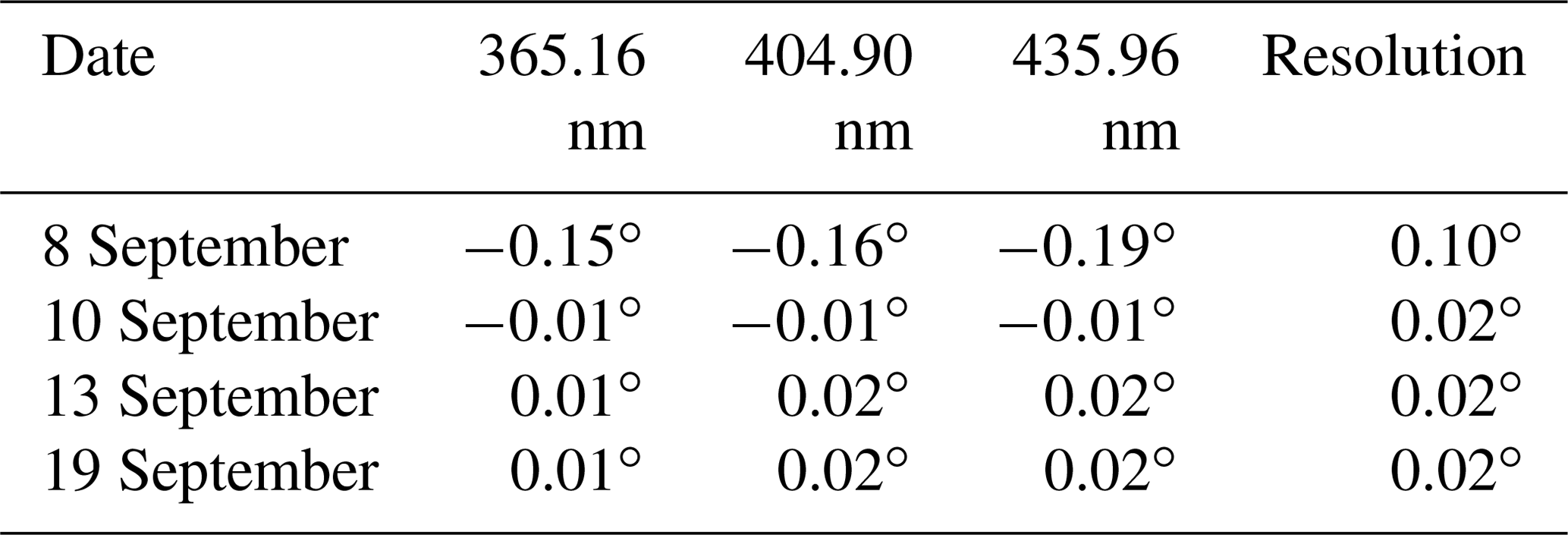
Table 2Overview of the lamp elevations obtained for all days and different wavelengths for the MPIC instrument. Additionally, the scan resolution is indicated in the last column.
In order to determine the elevation angle under which the xenon lamp could be seen, the centre of the intensity curve (dashed blue line in Fig. 4b) is calculated using the centre of mass formula:
where si denotes the intensity measured at the elevation angle αi. Using this equation yields a lamp elevation of 0.02∘ for the intensity curve shown in Fig. 4b. Here, it should be noted that Fig. 4b shows the intensity curve of an elevation scan that was performed by approaching the elevation angles from below. For scans where the angles were approached from above, the centres are found consistently at lower elevations by around 0.4∘. Because of that, we assured that all elevation angles were approached from below for the other calibration exercises since this was the scanning direction prescribed by the regular measurement protocol. It should be mentioned that depending on the kind of stepper or motor, not all instruments suffered from such backlash issues. Some, actively corrected for this by using inclinometers (e.g. LMU and IUP-HD) or active sun trackers (e.g. BIRA). Besides that, most of the instruments which experienced backlash issues solved them by simply scanning always from the same direction (in elevation and azimuth direction). The effect of backlash (maximum difference between both scanning directions) ranges from fractions of a degree to roughly 1∘. While this effect is very important for the elevations of the instruments, the effect has a much smaller influence on the measurements in the azimuth direction.
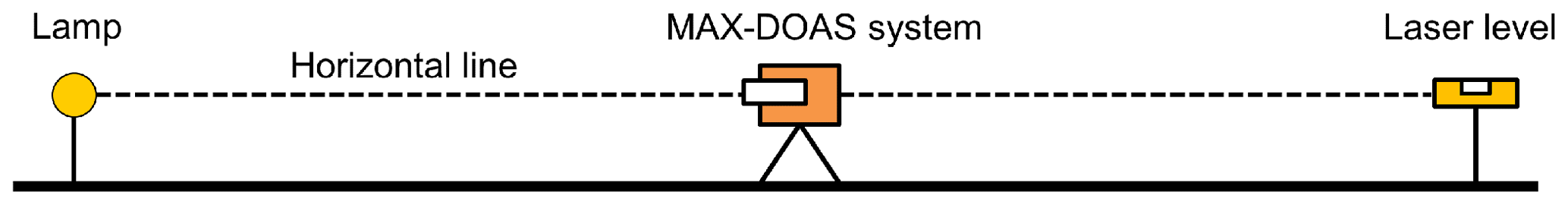
Figure 6Sketch of the measurement setup for the near-lamp measurements and the alignment of telescope and lamp.

Figure 7Measured intensities for the three individual scans (coloured dots) and the fitted Gaussian (red solid line) obtained from the near-lamp measurements by the IUP-HD instrument in the UV spectral range.
Equation (1) is used to calculate the centres of the intensity curves for all three wavelengths and all 4 d. The corresponding lamp positions are summarised in Table 2. Taking into account that the minimum motor step size is 0.01∘, the different values are consistent with each other within the span from −0.01 to 0.02∘ (excluding 8 September, when the scan resolution was only 0.1∘). Here, it should be noted that the centre of a Gaussian fit (see red fit curve in Fig. 4b) yields consistent lamp elevations compared to the centre of mass approach which was applied here. Therefore, also for the MPIC instrument, a Gaussian fit is used in Sect. 4.1, where the lamp scans of all instruments are analysed in a consistent way.
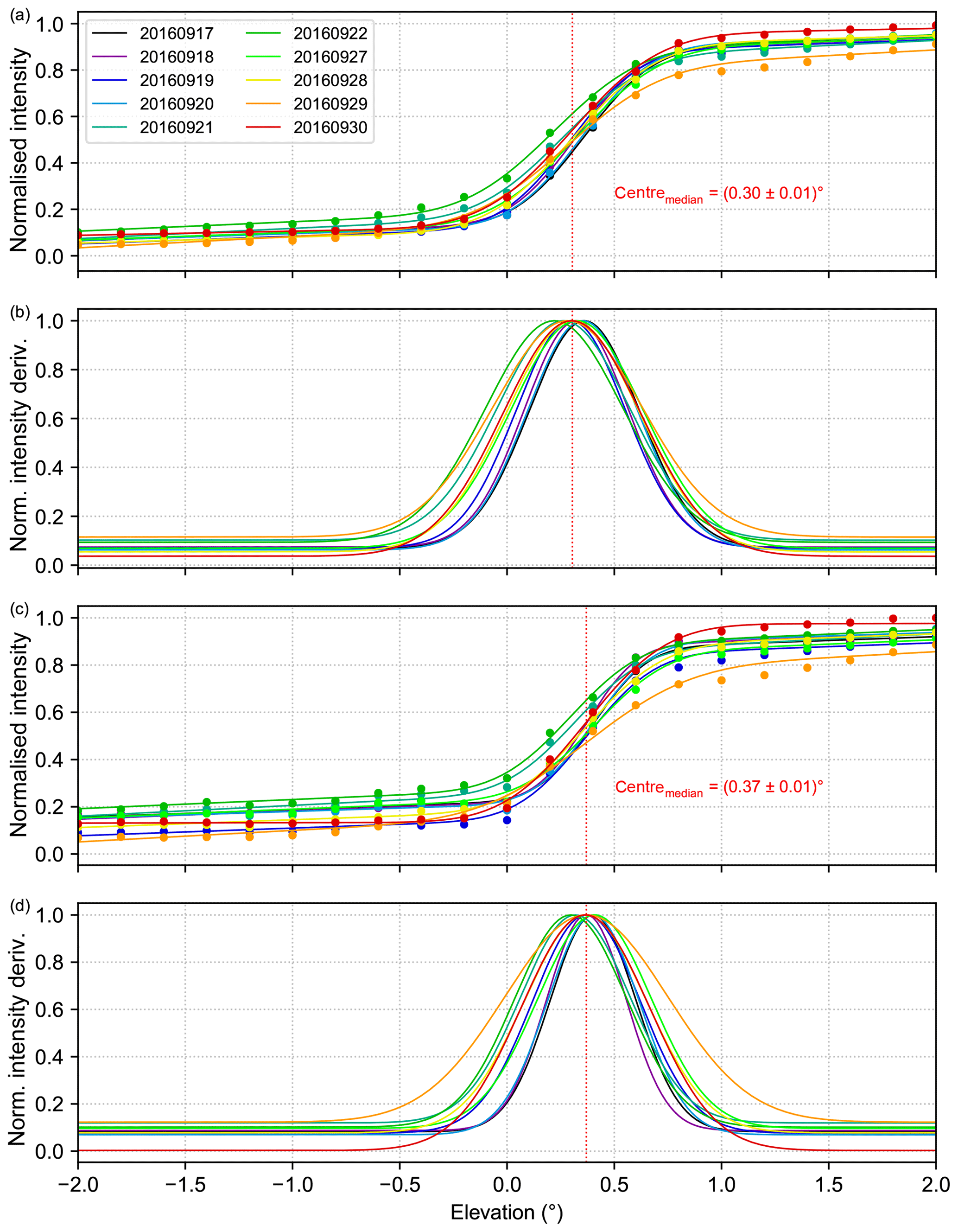
Figure 8Panels (a) and (c) show the normalised intensity curves for the horizon scans performed by the MPIC instrument throughout the campaign at 340 and 440 nm, respectively. The coloured solid lines indicate the respective Gaussian integral fits. Panels (b) and (d) show the normalised derivatives of the respective intensity curves. The median centres of the horizon scans are represented by the dashed red lines.
As already mentioned above, the position of the artificial light source relative to the instrument has to be known very accurately in order to calibrate the elevation angles of the MAX-DOAS system. Based on the setup summarised in Fig. 3, an expected lamp elevation of around is obtained, when using an estimated height difference, Δh, of 1 m between the xenon lamp and the telescope unit. The total error in the determination of the lamp mark (error of ±0.2 m) and the height difference Δh (error of ±0.3 m) is estimated to be around ±0.5 m, which translates to an uncertainty of in the expected lamp position. Further, the Earth's curvature at a distance of 1280 m corresponds already to and is therefore not negligible. Adding this offset to the obtained lamp elevation, the MPIC MAX-DOAS system should find the lamp at around elevation. If we compare this value to the values given in Table 2, we can conclude that the instrument sees the lamp close to the expected position. The small deviations between the table values and the expected elevation can be explained by a combination of several small uncertainties, namely the minimum motor step size of 0.01∘, the used scan resolution of 0.02∘ and the uncertainties of the calculation of the lamp position using Eq. (1). Further, also the determination of the expected lamp elevation has an uncertainty as outlined above.
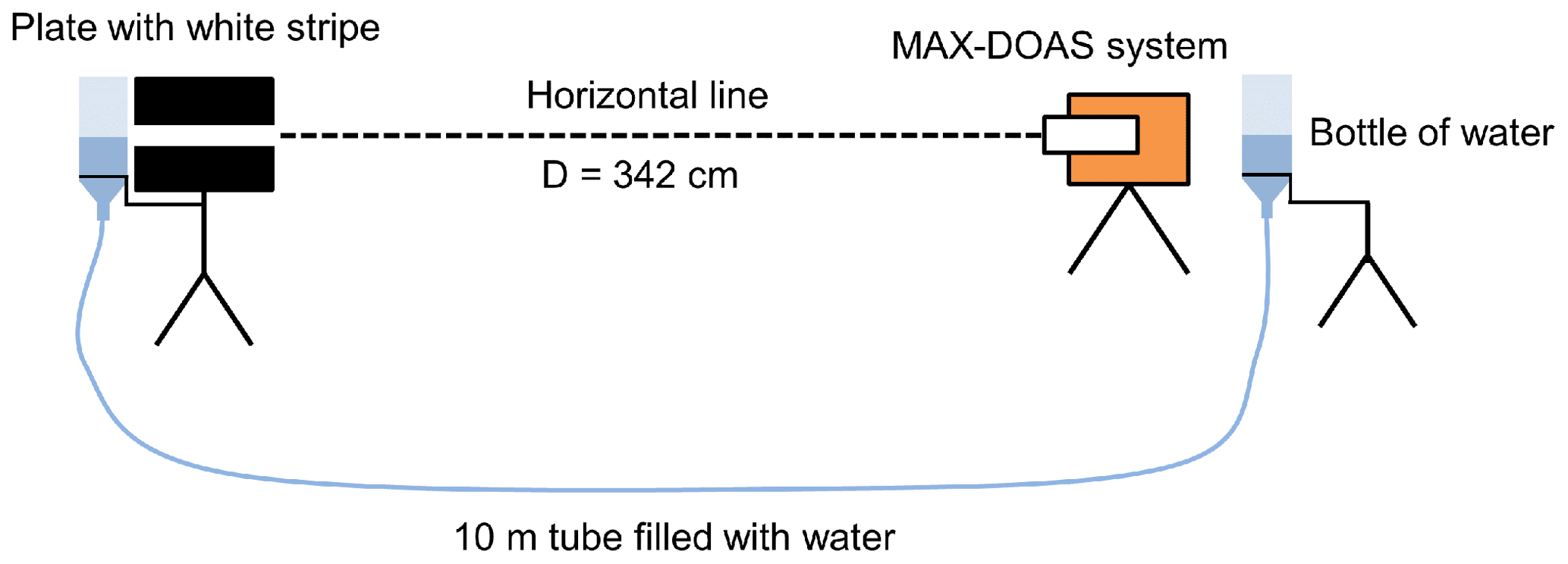
Figure 9Sketch of the measurement setup used by MPIC for the white-stripe scans and the alignment of the telescope and white stripe using a water level.
The relatively small span of lamp positions obtained on different days and at multiple wavelengths indicates that this method is very stable and reproducible. Furthermore, this approach allows for the calibration of several instruments with the same setup at the same time, since all instruments can point at the same target. However, depending on the slight horizontal distances of the different measurement locations, small differences in the azimuth angle (up to 1.8∘ for the CINDI-2 campaign) under which the lamp can be seen have to be taken into account. A drawback of this method is that the position of the artificial light source relative to the instrument has to be determined accurately, which might be challenging or even impossible at some locations. Also, finding a suitable location for the lamp can be difficult, e.g. in cities.
3.3 Near-lamp measurements
3.3.1 Approach
This method also uses an artificial light source (mercury-vapour lamp) during nighttime, but here it is located rather close to the instrument's telescope (a few metres). In order to determine the expected lamp position, namely , the light source has to be aligned to the (centre of the) telescope unit of the instrument. This alignment is typically done using a laser level which illuminates both the instrument and the position of the lamp. The telescope and the lamp are then centred around the position of the laser beam. The levelling accuracy of the laser level which was used during CINDI-2 was tested in the laboratory and amounts to approximately 0.1∘. Further, the laser beam has a thickness of about 2 mm, which translates to another 0.04∘ uncertainty in the relative vertical positions between instrument and lamp. Both the setup and the alignment procedure are sketched in Fig. 6. Using this procedure, the light source should be found at 0∘ elevation and possible deviations from that position can be used to correct the elevation calibration.
Such near-lamp measurements were not performed for the MPIC instrument during the CINDI-2 campaign. However, the elevation angles of the IUP-HD instrument were calibrated using this method. Therefore, in the following, data from the IUP-HD instrument are used to illustrate this method and its analysis in more detail.
3.3.2 Results for the IUP-HD instrument
Three such near-lamp scans were done by the IUP-HD group in one night in the preparation phase of the CINDI-2 campaign. Mean intensities are calculated separately for the UV and VIS spectrometers of the IUP-HD instrument. The first two scans were performed in an elevation range from −2 to 2∘, while the last was done in a range from −1 to 0.45∘. Since the elevation pointing is continuously regulated by comparison of the orientation of the telescope measured by the built-in tilt sensor with the nominal angle, no backlash effects are expected. In order to analyse these measurements, the (normalised) mean intensities are plotted against the elevation angle α reported by the measuring system. Next, a Gaussian function of the form
is fitted to the intensities and the centre of this function represents the lamp elevation. Further, S(α) represents the fitted intensity at a given elevation, A represents an intensity offset and B describes the maximum of the fitted curve. The width of the fitted curve is controlled by the parameter σ. For improving the statistics, all three scans are plotted in one plot (using different colours for the individual scans), and the Gaussian fit is applied to the whole data set of one spectrometer (Fig. 7).
The retrieved lamp elevation is also shown in this figure. Following this procedure, lamp elevations of −0.14 and were found in the UV and visible spectral range, respectively. These lamp elevations can now be used to adjust the initial elevation calibration of the instrument.
3.4 Horizon scans
3.4.1 Approach
A common method for the calibration of the elevation angles of MAX-DOAS systems is the so-called horizon scan. Here, the elevation β of the visible horizon, which is defined as the transition of the tree tops to the open sky, is used as reference. Since this method does not require an active light source, it can be performed during daytime and the variation in the measured intensity at the horizon is used to determine its position. A Gaussian integral is fitted to the measured intensities and the fit parameters give the horizon position. In practice, sometimes the numerical derivative of the intensity curve is calculated since below the horizon the intensity does not approach zero but the rapid change of the measured intensity allows for the identification of the horizon position . Prerequisites of this method (despite the knowledge of the expected elevation of the visible horizon) are high visibility, the absence of rapidly varying and/or low-lying clouds, and a clear and rapid change in intensity at the visible horizon, which might not be fulfilled during episodes of fog, when the horizon might be blurred. If these conditions are not fulfilled, no clear conclusions can be drawn from horizon scans. Furthermore, the visible horizon should not be too far away (less than a few kilometres) to minimise the influence of atmospheric scattering.
During the CINDI-2 campaign, horizon scans were included in the measurement protocol in order to study the consistency and stability of the elevation calibration of the different measurement systems. Thus, all MAX-DOAS instruments (both 1-D and 2-D) performed horizon scans between 11:40 and 11:45 UTC at a specified total integration time of 5 s while pointing in the main viewing direction (287∘ azimuth angle). The scans were done using predefined elevation angles between and 5∘, whereby the scan resolution was 0.2∘ in the interval between −2∘ and 2∘ and 1∘ outside this range.
3.4.2 Results for the MPIC instrument
For the MPIC instrument, horizon scan data are available starting from 17 September until 2 October. Before 17 September some horizon scans were performed as well, but they are of limited quality due to an error in the measurement script of the MPIC system. Further, some days are not used either due to bad weather conditions with fog and many low clouds or due to known pointing problems. Overall, useful horizon scan data are available on 10 d for the MPIC instrument.
First, the measured intensity is normalised with respect to the total integration time. As a second step, the intensity curves are also normalised to their corresponding maximum, allowing a direct comparison of the intensity curves recorded on different days with various sky conditions. The normalised intensity curves obtained at 340 nm for the different days are shown in Fig. 8a (coloured dots). Here, the increase in the measured intensity around the horizon is clearly visible in an elevation range from around 0 to 1∘. Next, a Gaussian integral of the form
is fitted to the data since this approach is more stable than calculating a numerical derivative. Here, S represents the fitted intensity; α the elevation angle; and the parameters A, B, C, and D determine the exact form of the fitted curve. The parameter indicates the centre of the fitted function and therefore represents the derived horizon elevation. The resulting daily fit functions are also displayed in Fig. 8a by lines in the corresponding colours.
Additionally, the analytical derivative of Eq. (3) can be calculated. The resulting curves, which are displayed in Fig. 8b, contain information on the instrument's field of view (FOV) since the full width at half maximum (FWHM), which is a typical measure for the FOV, can be derived:
By following this procedure, a value of 0.30∘ is found as the median centre (vertical red line in Fig. 8) for the fitted functions representing the median horizon elevation for the MPIC instrument at 340 nm. However, there is quite some scatter in the daily horizon scans, which might be caused by varying sky conditions on the different days and is one of the drawbacks of this method. The same procedure is also applied to the intensities recorded at 440 nm in order to study possible wavelength dependencies, the resulting intensity curves and derivatives are shown in Fig. 8c and d. Here, a median horizon elevation of 0.37∘ is obtained, which is slightly higher than the value for 340 nm. These two wavelengths were chosen for the analysis, because they were reported by all instruments that participated in the semi-blind intercomparison during the campaign, and thus they are well suited for a comparison of the horizon scan results for different instruments, which is explained in Sect. 4.2.
3.5 Bright or white-stripe scans
3.5.1 Approach
The white-stripe method can also be applied under daylight conditions and a white or at least bright stripe in front of a black or dark background is used as reference target. In order to calibrate the elevation angles, the (centre of the) white stripe has to be aligned with the (centre of the) telescope, archiving an expected stripe position of . This can be done by using a water or laser level.
The setup applied by MPIC during the CINDI-2 campaign used an adjustable white stripe in front of a dark plate and a large water level, which consisted of two bottles of water which were connected via a 10 m long tube filled with water and positioned next to the stripe and the telescope. On the telescope side, the water level has to be adjusted to the middle of the telescope; thus, on the plate stripe side the water level indicates the altitude of the telescope. Here, the stripe has to be adjusted to the water level position, which guarantees the alignment of stripe and telescope axis. A sketch of the described setup can be found in Fig. 9. The horizontal distance between the telescope and the white stripe was 342 cm, and the vertical extension of the stripe was around 2.5 cm, which corresponds to a FOV of around 0.4∘. This apparent FOV is quite large and shows that the setup was not optimised, but the rather short distance between telescope and stripe was determined by the local conditions (a water channel in front of the instrument container limited the maximum distance which could be achieved). Therefore, this calibration method using the here-described setup was applied only once during the campaign and only for the MPIC instrument. However, other groups (e.g. BIRA) applied the same method using their own setups. The scan resolution was 0.05∘, which was a compromise between speed (needed because of the unstable setup) and accuracy. In the following, the analysis is done for two wavelengths, namely 340 and 440 nm, in order to be consistent with the approach described in Sect. 3.4.
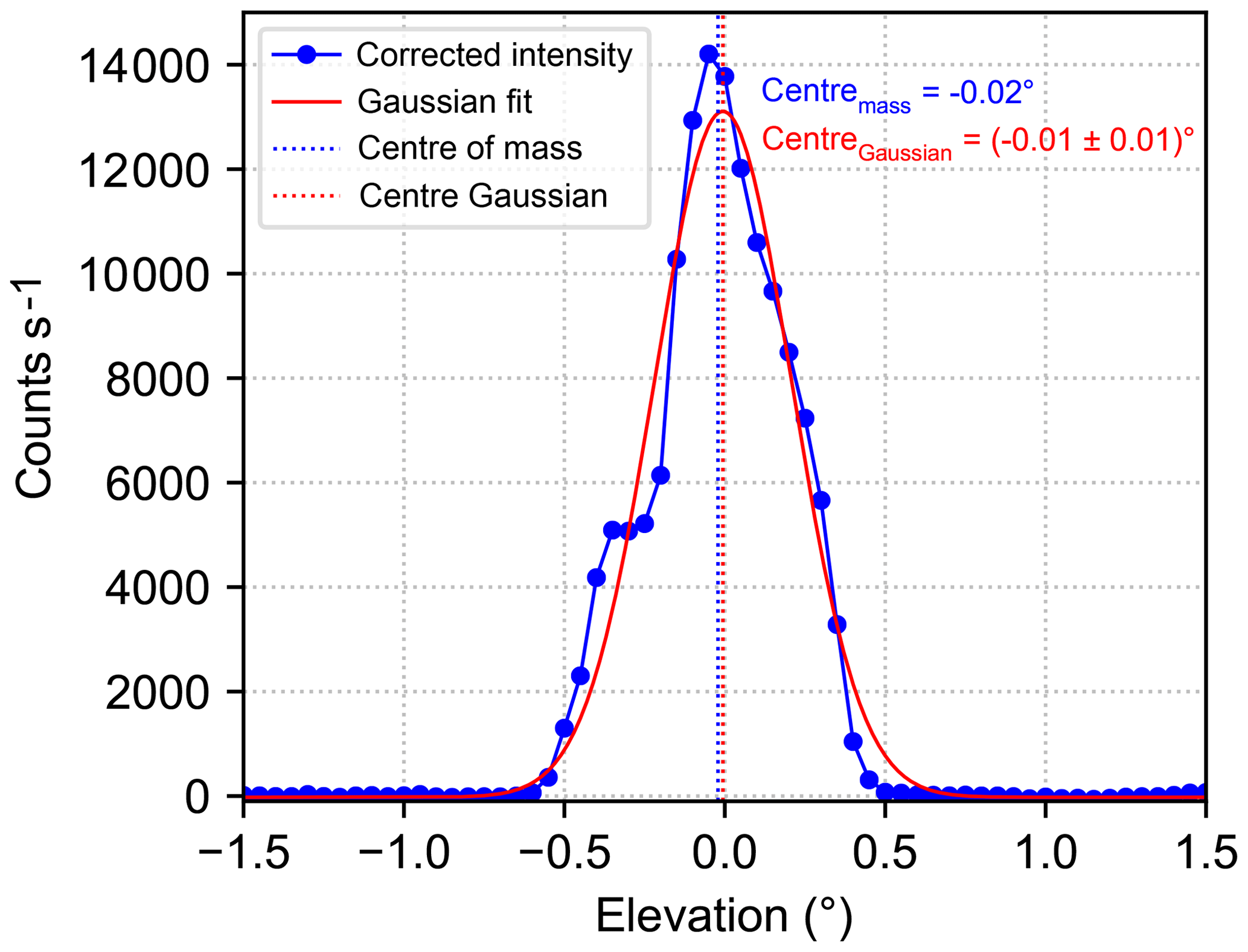
Figure 10Background-corrected intensity curve at 440 nm and corresponding Gaussian fit for the white-stripe scan on 20 September performed by the MPIC instrument. The retrieved apparent stripe positions for the two methods are indicated by the dashed lines.
3.5.2 Results for the MPIC instrument
Again, the recorded intensities are first normalised with respect to their total integration time. Next, a background correction is applied to the intensity curves, which is needed since the dark background of the white stripe does not absorb all incident light. For that, a second-order polynomial is fitted to the background intensities and subtracted from the measured intensities. The resulting intensity curve at 440 nm and the fitted Gaussian function (compare Eq. 2) are depicted in Fig. 10. Now, the centre of the Gaussian fit indicates the stripe position. In that way, a value of is found (dashed red line). Since the intensity curve again shows no smooth behaviour (see Sect. 3.2), additionally the centre of mass approach following Eq. (1) is applied, yielding a stripe position of (dashed blue line) consistent with the Gaussian approach. Conducting the same procedure for the intensities measured at 340 nm yields values of 0.02 and 0.00∘ for the Gaussian and centre of mass approaches, respectively.
In summary, a range of −0.02 to 0.02∘ for the retrieved stripe positions is obtained, which corresponds to only four motor steps. Similarly to the far-lamp measurements (Sect. 3.2), this range can be explained by the minimum motor step size of 0.01∘, the used scan resolution of 0.05∘ and the uncertainties of the retrieval of the stripe position . Further, an error of ±5 mm in the alignment between telescope and stripe was estimated, which translates to an uncertainty of . Finally, also the angular height (0.4∘) of the white stripe was quite large.
3.6 Sun scans
Sun scans use the solar disc as reference target. Its position is a function of time and the geolocation (longitude and latitude) of the instrument, and thus the expected position of the sun can be calculated with high accuracy. The position of the solar disc is described by two angles, namely the elevation angle and the azimuth angle. Therefore, this method can only be applied to 2-D instruments which allow for scans in these two directions. In order to determine the elevation angle (and the azimuth angle), under which the solar disc can be found, a scan across the solar disc (and its surrounding) similar to the methods described previously is performed. The retrieved value for , which was determined in the a priori elevation calibration, is then compared to the calculated elevation β and possible deviations can be corrected. Since also the azimuth angle of the sun can be determined, this method is also well suited to calibrate the azimuth angles of 2-D MAX-DOAS systems. This topic, however, is not part of this study and therefore not investigated in more detail here.
During the CINDI-2 campaign several 2-D instruments (e.g. BIRA, AUTH and the Pandora instruments, operated by KNMI, LuftBlick and NASA) performed sun scans to calibrate their elevation (and azimuth) angles. The Pandora systems performed sun scans on a regular basis to actively monitor and adjust their elevation (and azimuth) calibrations. As shown later, the results for these instruments show good agreement to the other presented calibration methods. Advantages and disadvantages of this method will be discussed in the conclusion section (Sect. 5) of this paper.
Table 3Overview of the retrieved target elevations for the MPIC instrument using three of the methods described in the text.

3.7 Comparison between the different methods
In this section, the different methods for the elevation calibration of MAX-DOAS instruments are compared and examined with respect to their consistency. Table 3 summarises the retrieved target elevations using the methods introduced above (except the near-lamp measurements and the sun scans, which were not done for the MPIC instrument).
A comparison of the results for the far-lamp measurements and the white-stripe scans shows very good agreement, with small deviations that can be explained by the already mentioned motor step size of 0.01∘, the different scan resolutions and the uncertainties related to the retrieval of the apparent target positions . For both methods, no significant wavelength dependence of the retrieved target positions is visible.
However, comparing the results for these two consistent methods to the results of the horizon scans shows larger deviations. The retrieved median horizon positions from the horizon scans for 340 and 440 nm were 0.30 and 0.37∘, respectively, which are significantly higher than the values around 0∘ found with the other two methods. During the campaign, the xenon lamp was placed directly in front of a row of trees which mark the visible horizon (the transition of the tree tops to the open sky). As already explained in Sect. 3.2, the vertical position of the lamp was 3.5 m above the water level in the water channel, which was located next to the measurement site (see Fig. 3), and a few metres below the tree tops. Thus, during the day the visible horizon is not represented by the ground but by the tree tops situated close to the lamp location in the main viewing direction of the MAX-DOAS instruments. Converting the retrieved horizon elevations of 0.30∘ and 0.37∘ (for 340 and 440 nm) into vertical distances at lamp location using geometry leads to heights of 6.7 and 8.3 m, respectively. The mean retrieved lamp position is 0.01∘, which corresponds to 0.22 m at lamp distance, and therefore the visible horizon is seen 6.5 and 8 m above the altitude of the lamp for 340 and 440 nm, respectively. These values are of the order of typical tree heights and therefore these calculations can explain the deviations (of about 0.30 to 0.37∘) from the other two methods. Later, this information is used to estimate the expected horizon elevation for the other instruments.
A further effect which can be observed for the horizon scans is that the median horizon elevation is significantly lower for 340 nm compared to the one obtained at 440 nm. As we will see in the next section, this effect is also found for the other participating MAX-DOAS systems. Besides this systematic wavelength dependency of the horizon scans, the results of the different methods agree quite well amongst each other when taking the uncertainties into account.
In this section the results of the far-lamp measurements and the horizon scans are inter-compared between the different participating groups.
4.1 Comparison of the far-lamp measurements
Far-lamp measurements using the xenon lamp as described in Sect. 3.2 were performed in several nights throughout the campaign. However, not all instruments participated each time. Since the different instruments use rather different instrumental setups and scanning schemes, they are divided into three groups.
4.1.1 Full 2-D scans
The first group consists of 2-D instruments which performed full 2-D scans of the xenon lamp in vertical (elevation angle) and horizontal (azimuth angle) direction on at least one night. For these instruments, the measured intensities are first normalised with respect to integration time and interpolated to specific wavelengths in order to compare the results of the different methods and instruments. Column (a) of Fig. 11 shows representative examples of the obtained 2-D intensity distributions for the BIRA, IUP-HD, UToronto and LMU (for this instrument only the mean intensities of the spectra are available) instruments, respectively. Additionally, black dotted lines indicating the azimuth angle under which the maximum intensity was recorded can be found in these figures. The axes of these sub-figures were chosen in a way that they all show the same relative elevation (1∘) and azimuth span (1.2∘). While the BIRA instrument shows a very smooth and smeared-out distribution of the measured intensities; the intensity distributions are more sharp for the UToronto (still quite smooth), IUP-HD and LMU instruments. This finding can be explained by the fibre configurations inside the telescope units of the four instruments since they have an influence on the actual shape of the measured intensity distributions. While the LMU and IUP-HD instruments used a ring of fibres inside their telescope units (for the UV channel), the UToronto and the BIRA UV instruments used a spot configuration, consisting of 37 and 51 fibres, respectively. When scanning across the xenon lamp, it might occur that the FOV is not always fully illuminated at the “edges” of the xenon lamp light beam. The ring configuration might be more sensitive (similarly to the fibre effect found for the MPIC instrument in Sect. 3.2) to this effect and introduce more edges to the measured 2-D intensity distributions, leading to a sharper shape. Further, differences in the motor pointing precisions have an effect on the apparent FOVs.
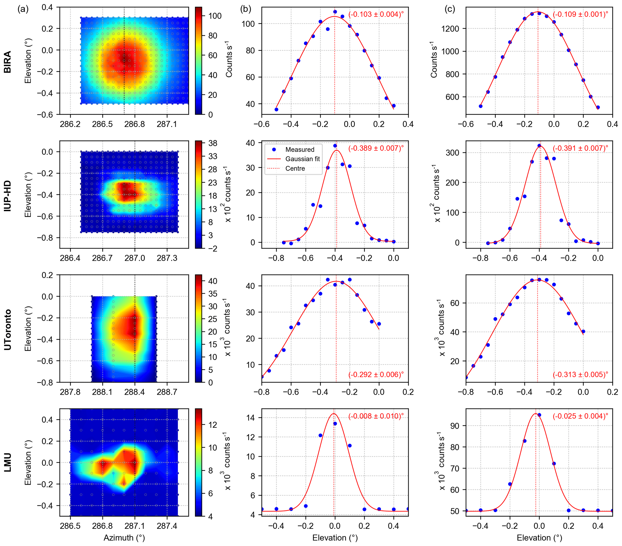
Figure 11(a) shows examples of the 2-D intensity distributions for the BIRA UV (at 365 nm, measured on 10 September), IUP-HD UV (at 365 nm, measured on 13 September), UToronto (at 436 nm, measured on 10 September) and LMU (mean intensity, measured on 10 September) instruments. (b) and (c) show the corresponding transects along the dashed black lines in (a) and the azimuthal sum of the intensities at the different elevations, respectively. Additionally, the respective Gaussian fits and their centres are indicated.
Two approaches were applied to retrieve the elevation under which the lamp is found for this first group of instruments. For the first approach, the intensities along a transect (black dotted lines in column a) are extracted and a Gaussian function (Eq. 2) is fitted to these intensities. The centres of these fits represent the lamp elevations; the intensity curves and Gaussian fits for the four examples can be found in column (b) of Fig. 11. For the second approach, all intensities which were recorded at one specific elevation angle are integrated over the different azimuth angles. These values are then used for the analysis, and again the centre of a Gaussian fit indicates the vertical position of the light source. Column (c) of Fig. 11 depicts the resulting curves and fits for the four instruments. The results of the two methods are very consistent for a single instrument. Nevertheless, there is quite some spread between the different instruments, which will be investigated in more detail at the end of this section.
4.1.2 Cross-scans
The second group contains 2-D instruments which performed cross-scans, meaning that first an azimuth scan was performed followed by an elevation scan at the azimuth direction under which the maximum intensity was found. This was done by three instruments using individual scanning schemes. Examples of the obtained intensity curves and corresponding Gaussian fits are depicted in Fig. 12. The different panels of this figure show the curves; fits; and resulting centres for the AUTH (a), BOKU (b), and IUP-B (c) instruments, respectively. The results for the lamp position are rather consistent for the different scans for an individual instrument since the obtained centres are nearly the same. This is also valid when looking at the results for different wavelengths for one instrument (not shown here). However, it can be seen that there is some spread between the different instruments.

Figure 12(a) Intensity curves at 365 nm recorded on 10 September by the AUTH instrument. (b) Intensity curves at 546 nm recorded on 13 September by the BOKU instrument. (c) Intensity curve at 546 nm recorded on 13 September by the IUP-B visible instrument.
4.1.3 1-D scans
The last group consists of 1-D instruments which performed simple elevation scans of the xenon lamp as described in Sect. 3.2. For these instruments, the normalised intensity is plotted against the elevation angle, and the centre of a Gaussian fit gives the lamp elevation. Examples for the CMA_UV, CMA_VIS, BSU and AIOFM instruments are shown in Fig. 13, with the resulting lamp elevations (centres) also displayed. Since the BSU instrument has a 2-D CCD on which the second dimension represents the elevation angle, this instrument did not really scan across the lamp, but each image on the CCD represents a full lamp scan. The AIOFM instrument is a 2-D instrument, but it was operated in 1-D mode for the far-lamp measurements.
4.1.4 Analysis of the far-lamp scans
For each participating instrument, the intensity curves are extracted for all valid lamp measurements by applying the respective procedure explained above for different wavelengths (365, 405, 436 and 546 nm) corresponding to the individual spectral ranges of the instruments. Further, a Gaussian function (Eq. 2) is fitted to the data. The fit parameters are initialised by A0=0, B0=maximum of the measured intensity curve, (calculated using Eq. 1) and .
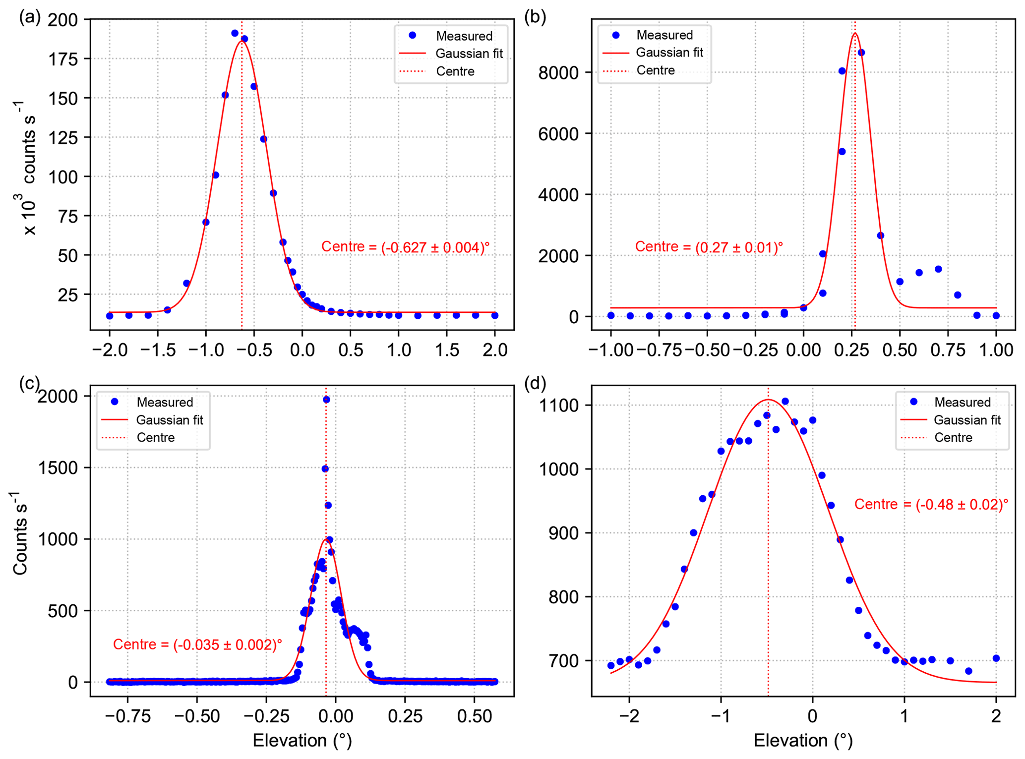
Figure 13(a) Intensity curve at 436 nm recorded on 19 September by the CMA_UV instrument. (b) Intensity curve at 546 nm recorded on 19 September by the CMA_VIS instrument. (c) Intensity curve at 365 nm recorded on 10 September by the BSU instrument. (d) Intensity curve at 365 nm recorded on 8 September by the AIOFM instrument.
The resulting lamp elevations are summarised in Fig. 14, where the mean of all retrieved lamp elevations (at different wavelengths, scans and/or days) for each instrument is shown as dots. Further, for each instrument, three different measures for the uncertainties of the retrieved lamp elevations are displayed. The left error bar of each instrument indicates the mean of all fit errors of the fits explained above and measures the quality of the individual fits and the shape of the measured curves. The standard error of the mean of all retrieved lamp elevations is represented by the middle error bar. It is a measure of the consistency and stability of the results of the different lamp scans performed by one instrument. This quantity also depends on the actual number of available intensity curves at different wavelengths and days, which is given in brackets behind the institute acronyms on the x axis in Fig. 14. Lastly, the right error bar indicates the daily spread, which is only available for instruments which performed more than one scan on 1 d and for all 2-D instruments, since two methods were applied to extract the 1-D intensity curves. The daily spread of 1 d is defined as the standard deviation of the results of the different scans on that day. If in addition several days are available, the mean of the daily standard deviations is calculated and displayed.
As shown in Fig. 14, a rather high spread of around 0.9∘ is found for the retrieved lamp elevations. Nevertheless, the values are centred around the expected values of (dashed blue line) and (dashed green line) for the instruments located on the upper (mostly 2-D instruments) and lower (mostly 1-D instruments) row of containers installed at Cabauw, respectively. These expected values were calculated as described in Sect. 3.2, where a Δh of 1 m was estimated for the instruments located on the lower row of containers (Fig. 3). The instruments on the second row of containers are placed around 3 m higher than the instruments on the lower row, and therefore the same calculations yield an expected lamp position of . Further, most of the error bars for the individual instruments are quite small, indicating the good stability and repeatability of the far-lamp measurements. The large error bar for the mean fit error for the LMU instrument can be explained by a rather uneven intensity distribution, which leads to bad fit results in some cases.
The deviations between the different instruments are on the one hand caused by slightly different vertical positions (even if they are located on the same container level) of the instruments, since some of the instruments were mounted on tripods or similar devices, while other instruments were placed closer to the container roof. On the other hand, the deviations are also caused by the fact that all groups reported their elevation angles corresponding to their own elevation calibrations. Therefore, the spread of about 0.9∘ of the retrieved lamp elevations (for one container level) is a measure of variability between the elevation calibrations of the different instruments.
More details will be discussed in Sect. 4.3, where the derived lamp elevations are compared to the corresponding horizon elevations obtained from the daily horizon scans, which are inter-compared in the next section.
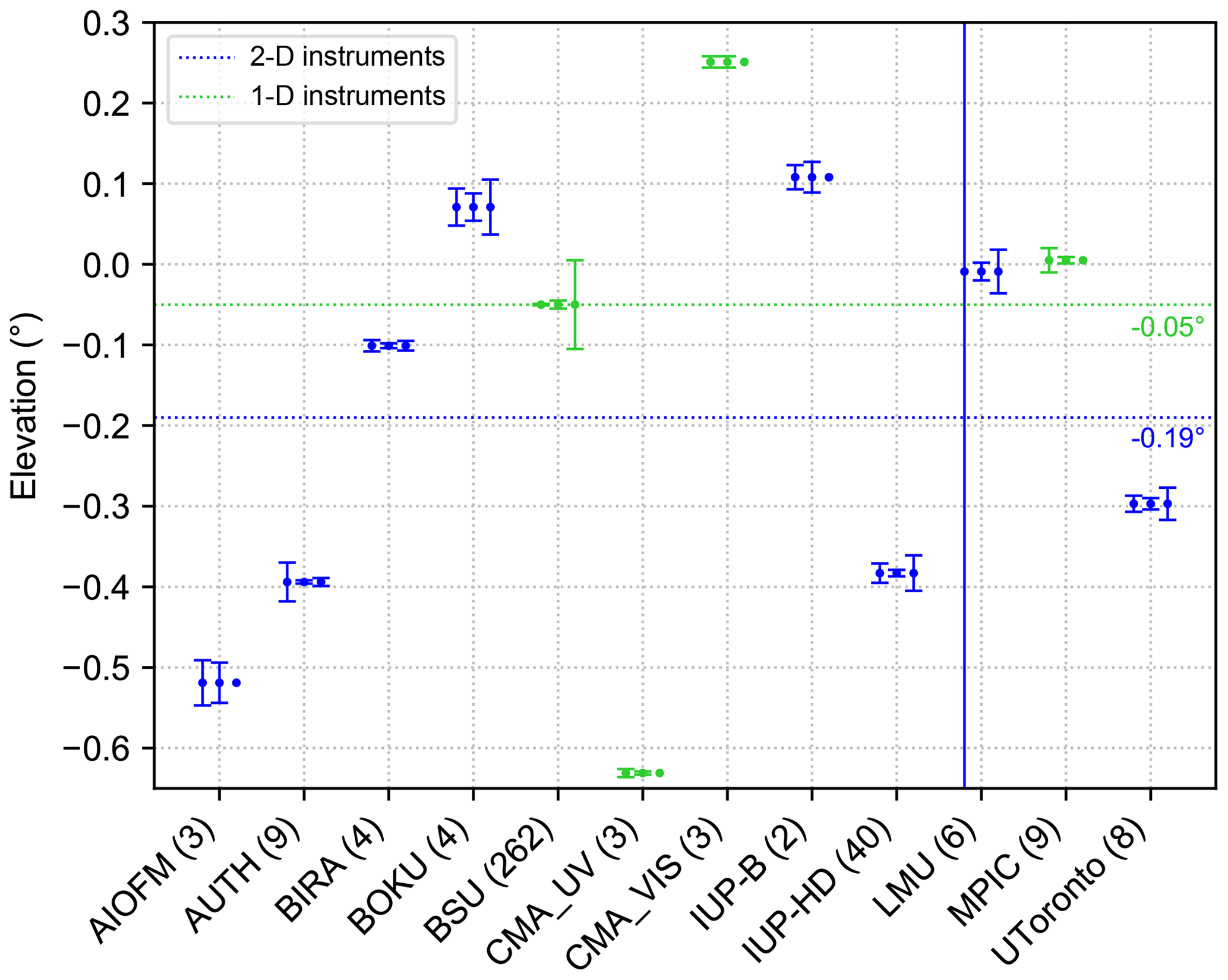
Figure 14Overview of the retrieved lamp elevations for the 2-D and 1-D instruments including different measures of their uncertainty, mean of fit errors (left), error of the mean (middle) and daily spread (right). The number of available lamp scans for each instrument is displayed in brackets after the individual institute acronyms. The expected lamp elevations are indicated by the corresponding dashed lines.
4.2 Comparison of the horizon scans
Already above it was mentioned that during the day the visible horizon might be defined by obstacles such as trees. As explained in Sect. 3.7 the horizon elevations of the MPIC instrument were used to estimate the height of the visible horizon above the lamp altitude, yielding values of 6.5 and 8 m at 340 and 440 nm, respectively. Taking into account the expected lamp elevations, which are slightly below 0∘ (Sect. 4.1), we estimate the elevation of the visible horizon to be 0.24∘ at 340 nm and 0.31∘ at 440 nm for the instruments on the lower row of containers. However, since some of the other instruments (mainly the 2-D ones) were located on the second row of containers, which was around 3 m above the lower row, the expected horizon elevation for these instruments is lower, and we derive elevations of 0.10 and 0.17∘ if we use the same assumptions. As we will see below, the difference between the estimated horizon elevations for the two rows is smaller than the spread of the results of the horizon scans between the individual instruments.

Figure 15Overview of the retrieved median horizon elevations for all participating instruments at the two different wavelengths. Additionally, the 25th and 75th percentiles are indicated by the lines.
In the following we use the results of the horizon scans of the participating instruments derived from the reported intensities of the daily horizon scans at 340 and 440 nm following the approach explained in Sect. 3.4 and Kreher et al. (2019).
First, median horizon elevations are calculated for both wavelengths for all instruments. These median values (dots) are depicted in Fig. 15 together with the corresponding 25th and 75th percentiles (lines), which are a measure of the spread of the daily horizon elevations. No percentiles are shown for the NIWA_EnviMeS instrument since horizon scans were reported only for 1 single day. The values at 340 nm are represented by blue dots and lines, while red dots and lines indicate the values at 440 nm. Additionally, the expected horizon elevations at 340 and 440 nm for the instruments on the upper container row are displayed as blue and red dotted lines, respectively. Only results for instruments which reported valid horizon scans on at least 1 d are shown.
Obviously, the retrieved horizon elevations of the different instruments have a quite large scatter of around 0.9∘, which is consistent with the spread of the lamp elevations that were discussed in the previous section. Nevertheless, the results for many instruments are centred around the estimated values from above. The results of the Pandora systems (operated by LuftBlick and NASA), which used sun scans to calibrate the elevation angles, are especially very close to that value. As indicated previously, the calculated difference of around 0.14∘ between the upper and lower rows in the elevation of the visible horizon is insignificant compared to the rather large scatter between the individual instruments. Even calculating mean or median horizon elevations for the instruments located on the upper and lower rows, which are displayed in Table 4, does not reveal this expected difference. When excluding some obvious outliers in the calculation of the mean (or median) elevations, there is some indication of this effect which would be, however, rather arbitrary.
Table 4Overview of the mean and median horizon elevations for the instruments located on the upper and lower row of containers and their corresponding standard deviations (SD).

Looking at the percentiles of the individual instruments shows that for many of them the results of the daily horizon scans have a high degree of consistency, which is indicated by the rather small percentile lines in Fig. 15. However, some instruments (e.g. the CMA instruments, the AUTH or the LMU instruments) show quite large percentile lines, indicating more variable results of the daily horizon scans. This finding can also be seen in Figs. 16 and 17, where the results of the horizon scans at 340 and 440 nm are displayed on a daily basis for the individual instruments (blue dots), together with the corresponding median (dashed blue lines) and expected (dashed black lines) horizon elevations. The instruments having small percentile lines show a smooth behaviour in the daily horizon elevations, while the ones having larger percentile lines show a higher dispersion (e.g. the CMA_UV instrument). Some of the instruments (e.g. the LMU instrument) show a systematic behaviour in the daily results, which might indicate adjustments to the elevation calibrations of these instruments, especially in the beginning of the campaign.
The rather large scatter between the instruments has several reasons. First, the individual instruments are placed at slightly different heights due to their specific instrumental setup even if they are located on the same container level. Further, the horizon is not a smooth line and the exact horizon position depends on the exact azimuth pointing direction and the actual shape of the horizontal line. Also, limited accuracy of the initial elevation calibrations of some instruments might contribute to this rather high dispersion of the horizon elevations. Lastly, also the weather (especially clouds) and visibility have a significant influence on the results of the horizon scans since they have an impact on the actual intensity variation around the visible horizon.
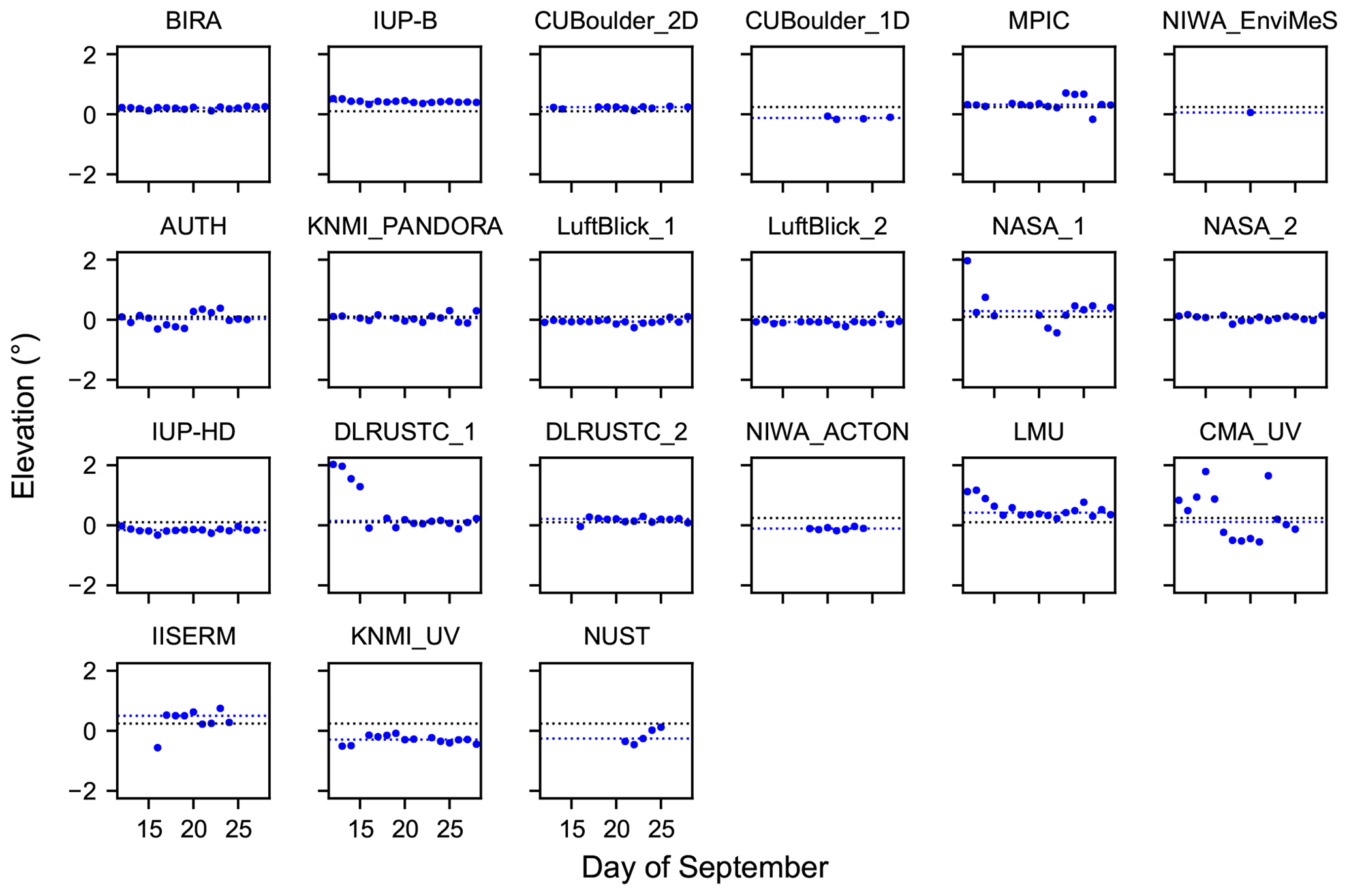
Figure 16Overview of the daily results of the horizon scans for all participating instruments at 340 nm. Additionally, in each subplot the median horizon elevation (dashed blue lines) and expected horizon elevation (dashed black lines) for the corresponding instrument are indicated.
Another finding is that the horizon at 340 nm is found at significantly lower elevations compared to 440 nm for most instruments which reported both intensities. However, it should be mentioned that for some instruments (e.g. the IUP-HD instrument), the different wavelength ranges are recorded using separated sensors and even separate optical entrance systems. Nevertheless, these instruments show the same systematic difference. This finding is consistent with the results obtained with the MPIC instrument, but so far no completely clear explanation could be found. An investigation of the intensity curves at different wavelengths for the horizon scan performed on 1 d shows an unexpected intensity variation at 0∘ elevation. An example is shown in Fig. 18a, which displays the normalised intensity curves at different wavelengths measured on 17 September (similar behaviours are found on other days). Here, a local minimum is visible at 0∘ elevation for wavelengths above 370 nm, which gets more pronounced for increasing wavelengths. This minimum influences the Gaussian integral fits (dashed lines in Fig. 18a), and the retrieved horizon elevations show a quite smooth wavelength dependence as depicted in Fig. 18b. These findings indicate a surface albedo effect. Pictures from the site show that in the visible spectral range the trees close to the horizon appear darker than the grass below them. This can be explained by the fact that the sun altitude is quite high during the horizon scans and the trees are illuminated at a rather flat angle, while the grass is illuminated in a very steep angle. In that way, the local minimum at 0∘ can be explained. However, it is not clear why at shorter wavelengths no such increase in the measured signal towards smaller elevation angles is found. Nevertheless, measurements which were collected during the first CINDI campaign support these indications for a surface albedo effect. Further, radiative transfer simulations showed that the wavelength dependence of atmospheric scattering cannot explain the observed wavelength dependence of the horizon scans. This unexpected wavelength dependence of the elevation scans is another drawback of the horizon scans, and if possible they should be analysed in the UV spectral range (at wavelengths below ca. 370 nm).
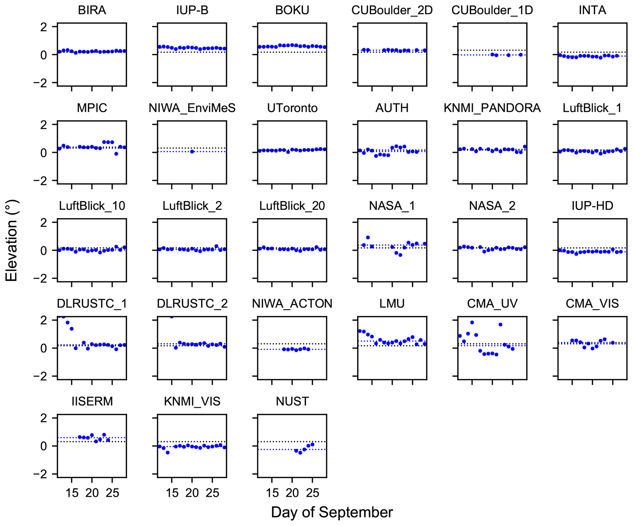
Figure 17Overview of the daily results of the horizon scans for all participating instruments at 440 nm. Additionally, in each subplot the median horizon elevation (dashed blue lines) and expected horizon elevation (dashed black lines) for the corresponding instrument are indicated.
4.3 Comparison between far-lamp and horizon elevations
Finally, the results for the far-lamp measurements and horizon scans are compared for all instruments which recorded far-lamp spectra and performed a horizon scan on at least 1 d. For that, the mean horizon elevations are plotted against the corresponding mean lamp elevations. This plot is done separately for the horizon elevations retrieved at 340 and 440 nm since a systematic difference for the results at the two wavelengths was found for the horizon scans. However, no such dependency was found for the lamp measurements. The resulting correlation plots can be found in Figs. 19 and 20, respectively. The error bars in the x and y directions indicate the standard errors of the mean retrieved lamp and horizon elevations, respectively.
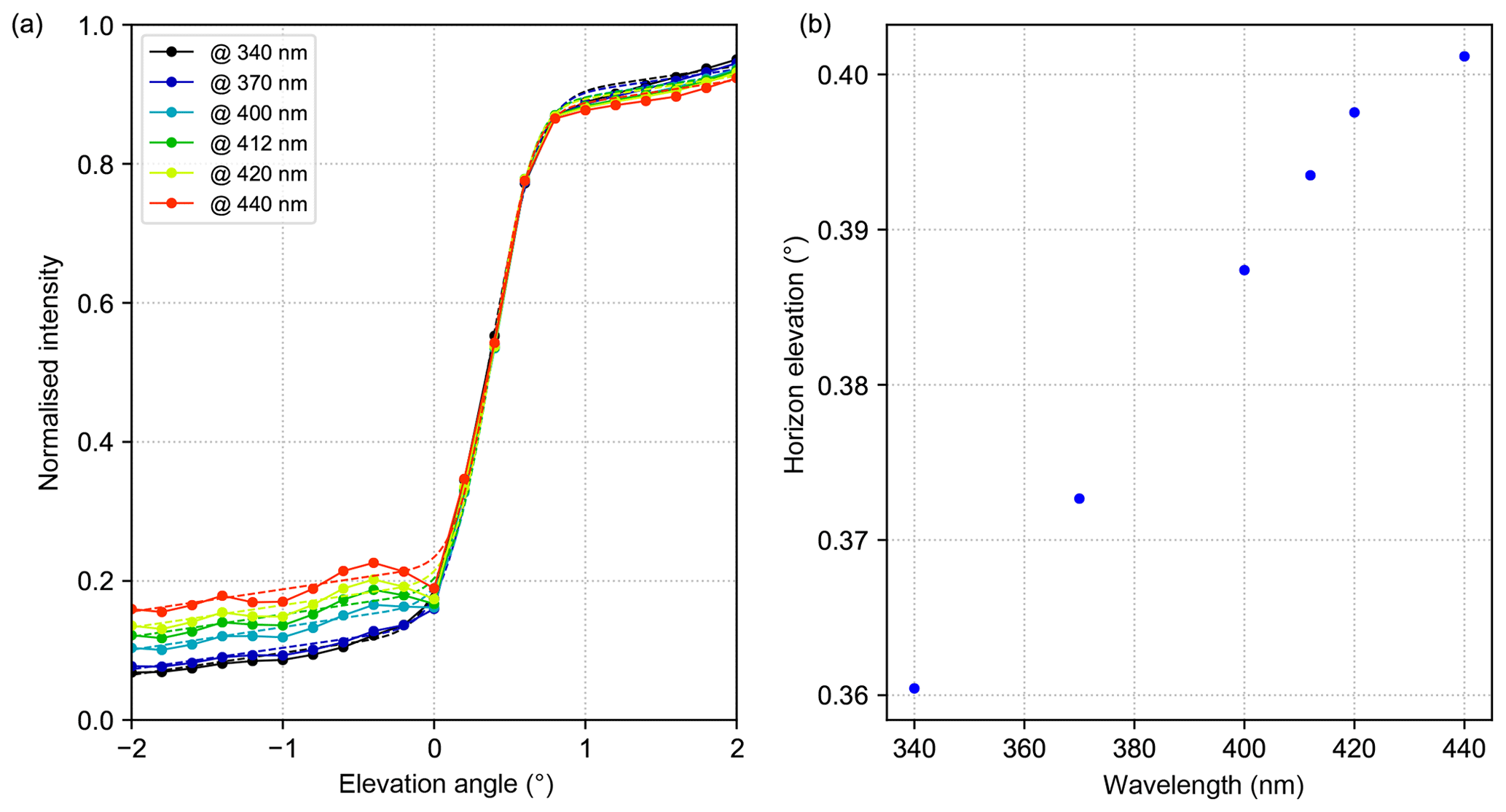
Figure 18(a) Normalised intensity curves (coloured dots) and corresponding Gaussian integral fits (coloured dashed lines) at different wavelengths for the horizon scan performed on 17 September by the MPIC instrument. (b) Respective horizon elevations (retrieved from the fits in a) as a function of wavelength.
A first finding is that the error bars are larger for the horizon scans for most of the instruments. On the one hand, this can be explained by the larger number of horizon scan measurements since most of the groups performed lamp measurements only on 1 or 2 d. On the other hand, however, the horizon scans are more sensitive to the different weather and sky conditions which influence the exact position of the visible horizon. Furthermore, the horizon is not a homogenous line and therefore uncertainties arise from the uncertainty in the exact azimuth angles of the different instruments. Lastly, for many of the instruments the horizon scans are performed at coarser resolution compared to the lamp scans, which also might effect the results and the resulting uncertainties.
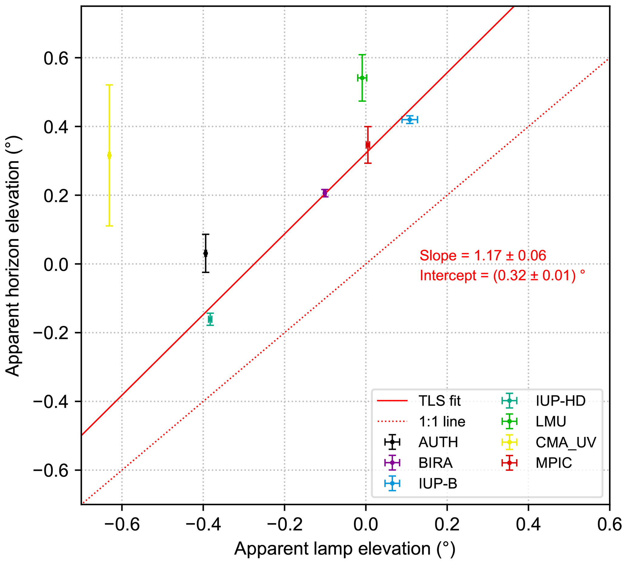
Figure 19Correlation between retrieved horizon (at 340 nm) and lamp elevations for all participating instruments that reported results for both methods. The error bars indicate the standard errors of the mean lamp and horizon elevations. Further, the result of a total least squares (TLS) fit and the 1:1 line are shown.
In order to examine the consistency between the two methods, a total least squares (TLS) fit (Cantrell, 2008) is applied to the data. This fitting method takes the uncertainties of the obtained values in both x and y directions into account by weighting the values with respect to their uncertainties. In that way values with a smaller uncertainty get more weight compared to those with a larger uncertainty. Here, the standard errors of the mean horizon and lamp elevations were used as measure of uncertainty. The resulting fit lines (solid red lines) with their corresponding slopes of 1.17 and 1.10 and their intercepts of 0.32 and 0.40∘ for 340 and 440 nm, respectively, are also displayed with their fit errors in the corresponding figures as well as the 1:1 line (dashed red line).
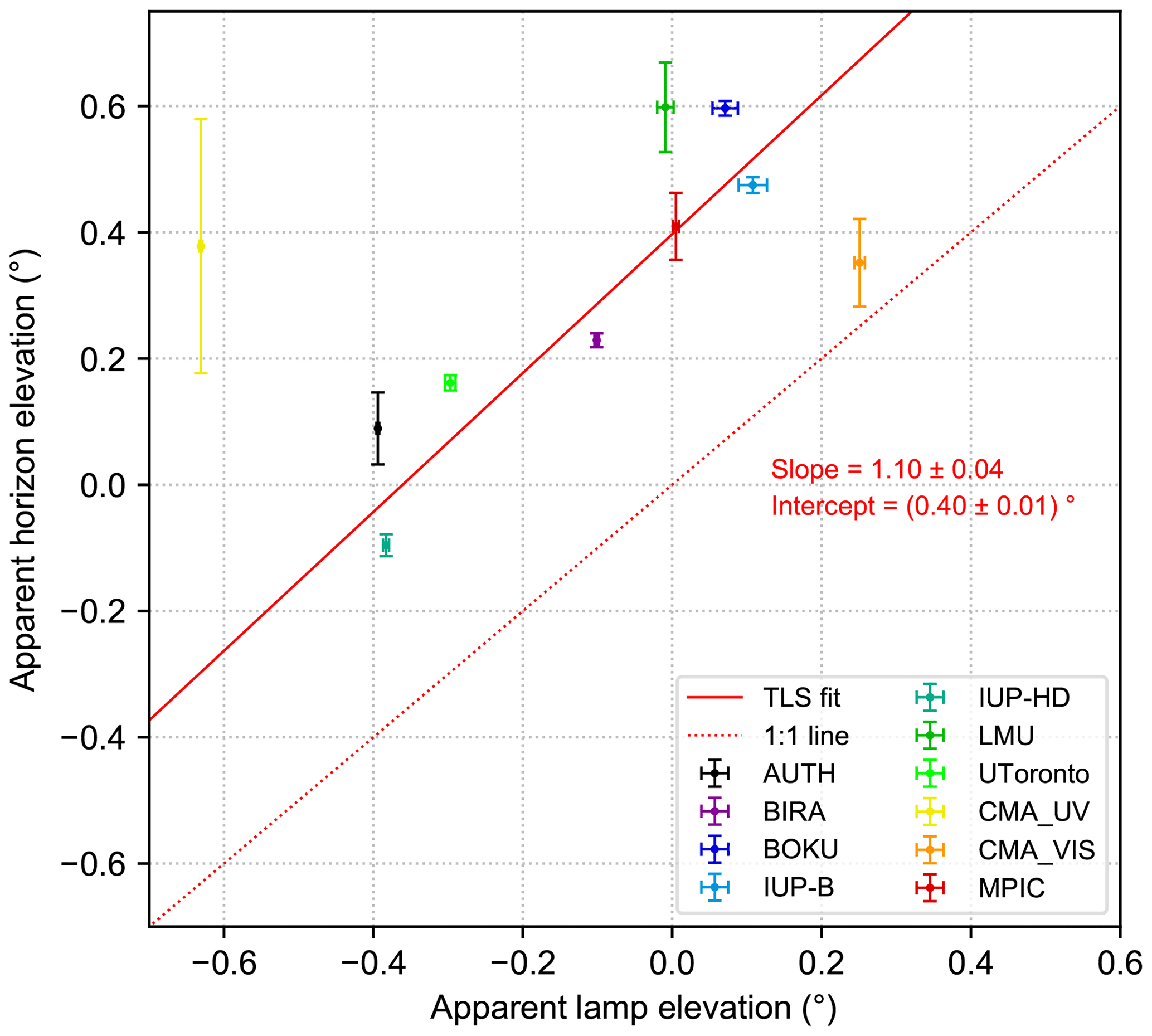
Figure 20Correlation between retrieved horizon (at 440 nm) and lamp elevations for all participating instruments that reported results for both methods. The error bars indicate the standard errors of the mean lamp and horizon elevations. Further, the result of a total least square (TLS) fit and the 1:1 line are shown.
Taking all the uncertainties of the two different methods into account, the slopes obtained by the TLS fits are close to 1, and we can state that the results of the two methods correlate well. Nevertheless, the horizon is consistently seen at around 0.2 to 0.6∘ (except the CMA_UV instrument, which has a very large error bar for the horizon scans) higher elevations compared to the lamp scans, which corresponds to around 4.5 to 13 m at lamp distance and is in agreement with the calculations in Sect. 3.7. As already described there, this systematic offset between horizon and lamp scans can be explained by the fact that during daytime the visible horizon is represented by trees. Further, this consistent offset between the two methods is represented by the intercepts of the TLS fits (0.32 and 0.40∘). Finally, the difference of 0.1∘ in the offsets obtained for the two wavelengths is consistent with the findings from Sects. 3.4 and 4.2.
All in all the two methods presented here yield consistent results for most of the instruments, and therefore both are suited to calibrate the elevation angles of MAX-DOAS systems.
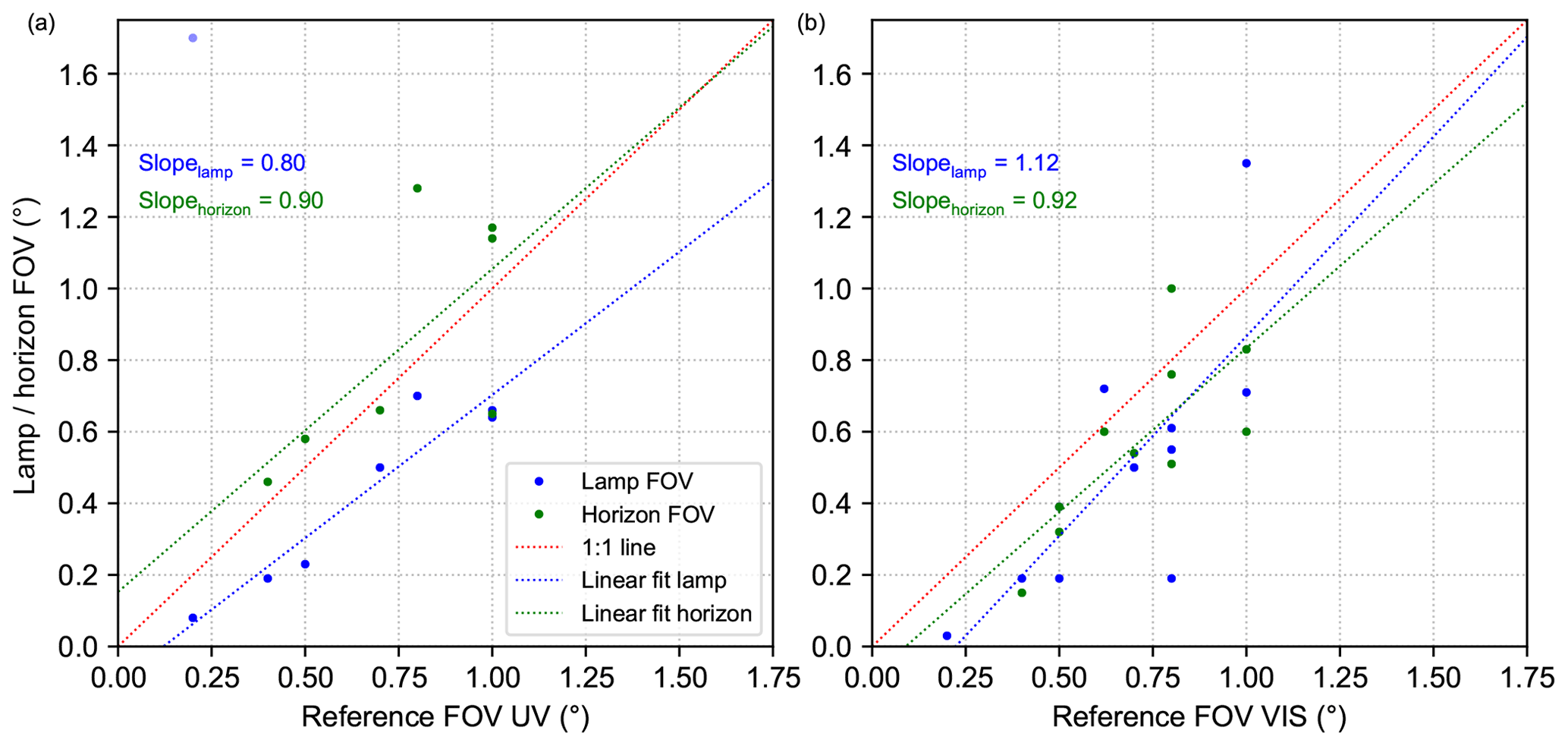
Figure 21Correlation between retrieved FOVs from horizon scans (green dots) and far-lamp measurements (blue) against their corresponding reference FOVs reported by the groups. Panel (a) shows the results for the UV spectral range, while panel (b) displays the same for the visible spectral range. In both plots linear regressions and 1:1 lines are included in the respective colours.
4.4 FOV determination
All presented methods use elevation scans across reference targets, and the apparent elevation angles under which the targets can be found are determined by fitting either a Gaussian function or a Gaussian integral. These fits also contain information on the fields of view (FOV) of the instruments, which are represented by the full widths at half maximum (FWHM). For the Gaussian integral, which was used for the horizon scans, the FWHM can be determined using Eq. (4). The FWHM for the Gaussian fit can be calculated using
where σ is the parameter controlling the width of the Gaussian function (Eq. 2), which is fitted as explained above. For the instruments which performed both far-lamp measurements and horizon scans, the FOVs were determined as outlined and compared to their reference FOVs, which were measured in the laboratory prior to the campaign and are listed in Table 1. The FOVs derived from the horizon scans and far-lamp measurements were plotted against the corresponding reference FOVs in Fig. 21. Here, blue dots indicate FOVs obtained from the far-lamp measurements, while green dots show the results retrieved from the horizon scans. Further, linear regressions (dashed blue and green lines) with their corresponding slopes and a 1:1 line (dashed red line) are shown. It should be noted that the results for the UToronto (not shown at all) and the AIOFM (pale blue dot in panel a) instruments were not included in the regressions since their retrieved FOVs are obviously problematic.
Both panels of Fig. 21 show that the results are not as clear as in the case of the determination of the horizon and lamp positions. This indicates that the centres which were retrieved so far, are more robust and less sensitive to the specific shape of the recorded intensity curves. Nevertheless, the obtained slopes of the regression lines are not that far from 1, which indicates that in principle the retrieval of the FOV from the elevation calibration methods is possible. However, especially in the visible spectral range, there seems to be a systematic underestimation of the retrieved FOVs as compared to the reference FOVs for most of the instruments. The reason for this is so far not clear and would need a more sophisticated assessment. This is, however, outside the scope of this paper since the focus of this paper is put on the elevation angle calibration. Another finding is that systematically slightly larger FOVs are found for the horizon scans compared to the lamp scans, especially in the UV spectral range. This can (at least for the 1-D instruments) be explained by the fact that the far lamp was not always in the centre of the azimuth dimension of the FOV for some instruments.
If the optical axis of a MAX-DOAS instrument would be precisely known, a simple water level could be used to calibrate the elevation angles. This assumption, however, is not always fulfilled, e.g. because the fibre bundle is not perfectly centred. Because of these uncertainties, the in-field calibration of the elevation angles as described in this paper is indispensable.
Five different methods for the calibration of elevation angles of MAX-DOAS instruments were described and discussed. All were applied during the CINDI-2 campaign by at least one group. The approaches of three methods were explained and examined using data from the MPIC MAX-DOAS instrument, while the near-lamp measurements were described using data from the IUP-HD instrument. White-stripe measurements, using the MPIC setup, were only done for the MPIC instrument. The results of the horizon scans and the far-lamp measurements were inter-compared quantitatively between the individual groups and amongst each other.
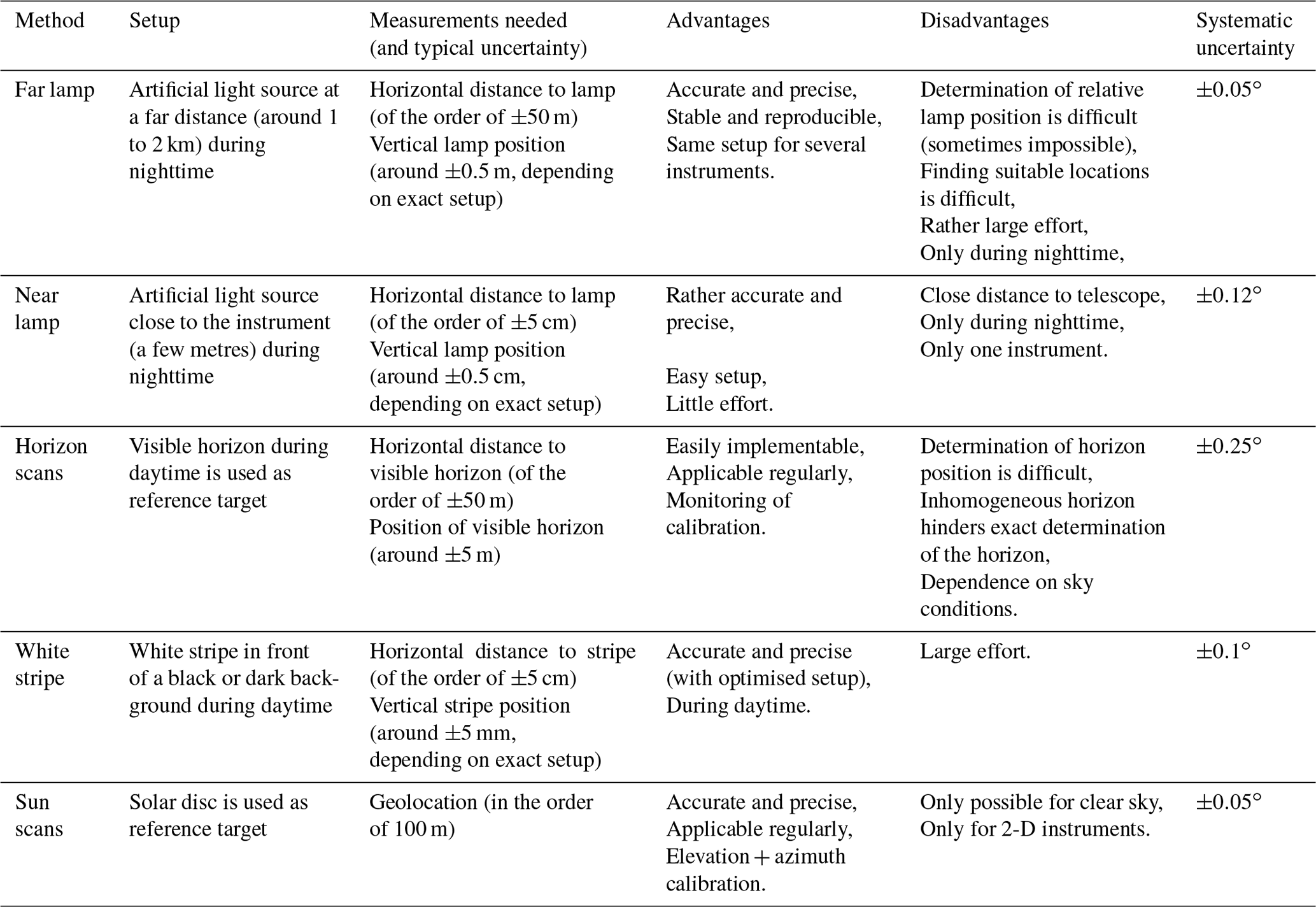
Table 5Overview on the basic characteristics of the described methods for elevation calibration. The table summarises the basic setup and prerequisites needed (column 2). Column 3 shows properties that have to be measured with their typical (systematic) uncertainties. Note that the uncertainties in this table are typical values and not the exact ones used in this study. Columns 4 and 5 list advantages and disadvantages of the different methods, respectively. Finally, the last column gives uncertainty estimates based on the results from CINDI-2 summarised in this paper. Here, it should be noted that also statistical errors occur, which are usually dominated by the uncertainties of the positioners (see Table A2). These uncertainties are usually between 0.02 and 0.1∘ and are similar for all methods.
All of the methods use the same principle. First, a specific target is placed in front of the telescope unit of a MAX-DOAS system. This target has to be located at a fixed and known location relative to the optical unit of the instrument. In that way, an expected elevation angle β under which the target should be found can be determined. Then the apparent elevation angle of the target is retrieved by the MAX-DOAS system using the measured intensities of an elevation scan across the target. Finally, the elevation angles of the instrument can be calibrated by comparing the expected and retrieved target positions and adjusting the telescope position in an appropriate way.
Tables A1 and A2 list systematic and statistical effects, respectively, which introduce uncertainties to the measurements and analyses presented in this paper. In summary it can be concluded that the systematic effects which determine the accuracy of a method are dominated by the uncertainties introduced during the determination of the target positions and the fit errors of the retrieval of the apparent target positions. The statistical errors which limit the precision of a method, however, are dominated by motor uncertainties. These are characteristic properties of the used motors and steppers of the individual instruments, and therefore the precision of the methods is prescribed by the individual properties of the motors and steppers (typically to ). In the following discussion the typical accuracy of each method is estimated by quadratically adding the (systematic) error related to the determination of the target position and the error associated with the Gaussian fits and then applying the square root. For the latter the values are ranging from ±0.01 to depending on the instrument and the symmetry of the recorded intensity curves. For that reason a value of is used in the following. However, for good-performing instruments, this value can be considerably lower and in many cases the accuracy of a method is simply limited by the uncertainties in the determination of the target position.
The first method used far-lamp measurements during nighttime, where an artificial light source close to the visible horizon was used as the target. The results for the MPIC instrument illustrate the stability and reproducibility of this method since similar results are obtained for the different days at multiple wavelengths. The results of the other groups confirm this finding since a rather small spread is found for each of the individual instruments. However, the spread of around 0.9∘ between all instruments is quite large, which is likely caused by the fact that the individual initial elevation calibrations are not done in a consistent way. As described in Sect. 3.2, the uncertainty associated with the determination of relative position of the far lamp is estimated to be ±0.5 m, which translates to at lamp distance. Combining this with the fit errors of the Gaussian fits yields a systematic uncertainty of the far-lamp measurements of . All in all, the main advantages of this method are the stability, reproducibility and the possibility to calibrate several instruments with the same setup. Furthermore, this method is very accurate as long as the instrument has a mostly symmetric FOV. For many instruments, the uncertainty is even smaller and is finally limited by the accuracy and precision of the motors of the instruments. Nevertheless, it might be difficult to find suitable lamp locations and to determine the position of the lamp relative to the telescope for most measurement sites. Therefore, the overall effort for this method is quite high. Lastly, this method can be applied only during nighttime. It should be mentioned that this method can also be used for calibrating the azimuth angles of 2-D instruments since also the azimuthal direction of the lamp can be determined; however, it might be difficult to find suitable lamp locations at different (azimuthal) locations.
Near-lamp measurements offer another way to perform an elevation calibration. This method is very similar to the far-lamp measurements, but here the lamp is located rather close to the instrument. Following the procedure above and using the uncertainties as outlined in Sect. 3.3, the systematic uncertainty of this method is estimated to be around . Like for the far-lamp measurements the main advantages are accuracy and stability. Furthermore, the setup is more compact and requires less effort, especially in determining the position of the lamp relative to the telescope. However, when comparing the typical accuracy of the near- and far-lamp measurements, the distance between the lamp and the telescope is quite small for the near-lamp measurements. This leads to a rather large angular fraction which is occupied by the lamp and influences the results of the lamp scan. Finally, this method can also be applied only during nighttime and only for one single instrument at once using the same setup.
Horizon scans during daytime use the visible horizon as target. Consistent results were found for all participating instruments compared to the far-lamp measurements. For both methods a spread of 0.9∘ between the individual instruments can be observed. Further, these consistent results are represented by a good correlation of the retrieved apparent horizon and lamp elevations. Here, the obtained slope is close to 1 and the obtained intercepts of 0.32 and 0.40∘ indicate an offset between lamp and horizon measurements. This offset can be explained by the fact that the visible horizon differed from the real horizon since trees represented the visible horizon during day. By knowing the height of these obstacles, this problem can be solved, and the offset between the method can be explained, as examined in Sects. 3.7 and 4.3. Additionally, it should be emphasised that the results of the horizon scans show a wavelength dependence (higher horizon elevations for larger wavelengths) which is likely caused by surface albedo effects and needs further investigation. Although the spread between the results for the different instruments is of the same order as for the far-lamp measurements, the spread for the individual instruments is significantly larger than for the lamp measurements. This is caused by the large sensitivity of the horizon scans to varying weather conditions and visibility. Further, more horizon scans were performed, which naturally increases the scatter in the retrieved horizon elevations since the scans were performed with different underlying sky conditions. Nevertheless, this method and its principle are quite simple and can be easily implemented in measurement protocols. Thus, this method can be easily performed on a regular basis and used for monitoring the elevation calibration. Altogether, this demonstrates that horizon scans are a good calibration method if only scans under favourable conditions are used and the position of the visible horizon is known. Hence, only days with good visibility should be used and days with rapidly varying cloud cover and/or low-lying clouds should be avoided. One major drawback is the difficulty to determine the height of the visible horizon, e.g. in mountainous regions. Also, for comparison exercises, it should be mentioned that the horizon is not a homogenous line but might have some inhomogeneities that can influence results for the individual instruments and therefore might introduce some discrepancies between the instruments. For the CINDI-2 campaign, the uncertainty of the determination of the position of the visible horizon was estimated as roughly ±5 m. Combining this with the fitting uncertainties yields a systematic uncertainty of the horizon scans of .
White-stripe measurements are another method which can be applied during the daytime. During the CINDI-2 campaign, the setup, which was used by MPIC, was rather experimental, and measurements using this setup were performed only by the MPIC instrument. Nevertheless, the results are promising and consistent with the other methods; also, other groups (e.g. BIRA) applied this method utilising a different setup. Since the position of the stripe relative to the optical unit can be determined very accurately, this method is very accurate. However, a stable setup is needed in order to perform a good calibration. For this method, a typical uncertainty of the order of is estimated, when using an error of ±5 mm in the determination of the strip position as explained in Sect. 3.5. But since only one such measurement was performed by the MPIC instrument, further studies are needed in order to confirm this estimate.
As discussed in Sect. 3.6, the errors introduced by the determination of the position of the solar disc can be neglected for the sun scans, and the systematic uncertainty is dominated by the retrieval of the apparent solar position and the motor properties. This is valid as long as the scans are performed when the sun altitude is large since otherwise atmospheric refraction might play a role. Therefore, we estimate the accuracy of this method to be typically of the order of . Like for the other methods the statistical uncertainties are given by the motor precision. Main advantages of this method are the high accuracy, the possibility to perform such sun scans regularly, and the option to calibrate both elevation and azimuth angles. Major disadvantages of this method are the fact that these scans can only be applied under cloud-free conditions and that this method is only applicable to 2-D instruments.
Table 5 provides a summary of the described methods by listing their setups, the measurements which are needed, their specific advantages and disadvantages, and their typical systematic uncertainties.
The results of this study show that in principle all of the presented methods can be used for the calibration of the elevation angles of MAX-DOAS systems since they yield consistent results. Nevertheless, the advantages and disadvantages of the individual methods should be considered when deciding for one method. A further finding of this study is the fact that still some improvement in the consistency of the elevation calibration between the different MAX-DOAS systems is needed as there is still a rather large discrepancy between the different instruments of around 0.9∘. This is of the order of a typical FOV of a MAX-DOAS system and might have a significant effect on the retrieved MAX-DOAS trace-gas dSCDs. Therefore, for upcoming campaigns, strong emphasis should be put on the monitoring and possible correction of the elevation calibration. To do so, if possible and if suitable lamp positions can be found, far-lamp measurements should be performed at least once by all participating instruments, and a common elevation reference (namely the lamp elevation) should be defined prior to a comparison campaign. In general we recommend that given the high accuracy, 2-D instruments should make use of sun scans. Simple 1-D instruments should perform near-lamp or white-stripe scans to accurately calibrate the elevation angles since these two methods are rather accurate and the effort is reasonable. As these two methods do not have a common reference elevation, they are more suitable for individual MAX-DOAS stations. Both during campaigns and for single MAX-DOAS stations, horizon scans (or sun scans for 2-D instruments) should be implemented in the measurement protocol and should be performed on a regular basis in order to monitor the temporal stability of the calibration of the elevation angles.
This section provides two tables which list and evaluate systematic (Table A1) and statistical errors (Table A2) that influence the measurements described in this paper and therefore cause uncertainties in the elevation calibration.
Table A1List and evaluation of systematic effects influencing the measurements presented in this paper.
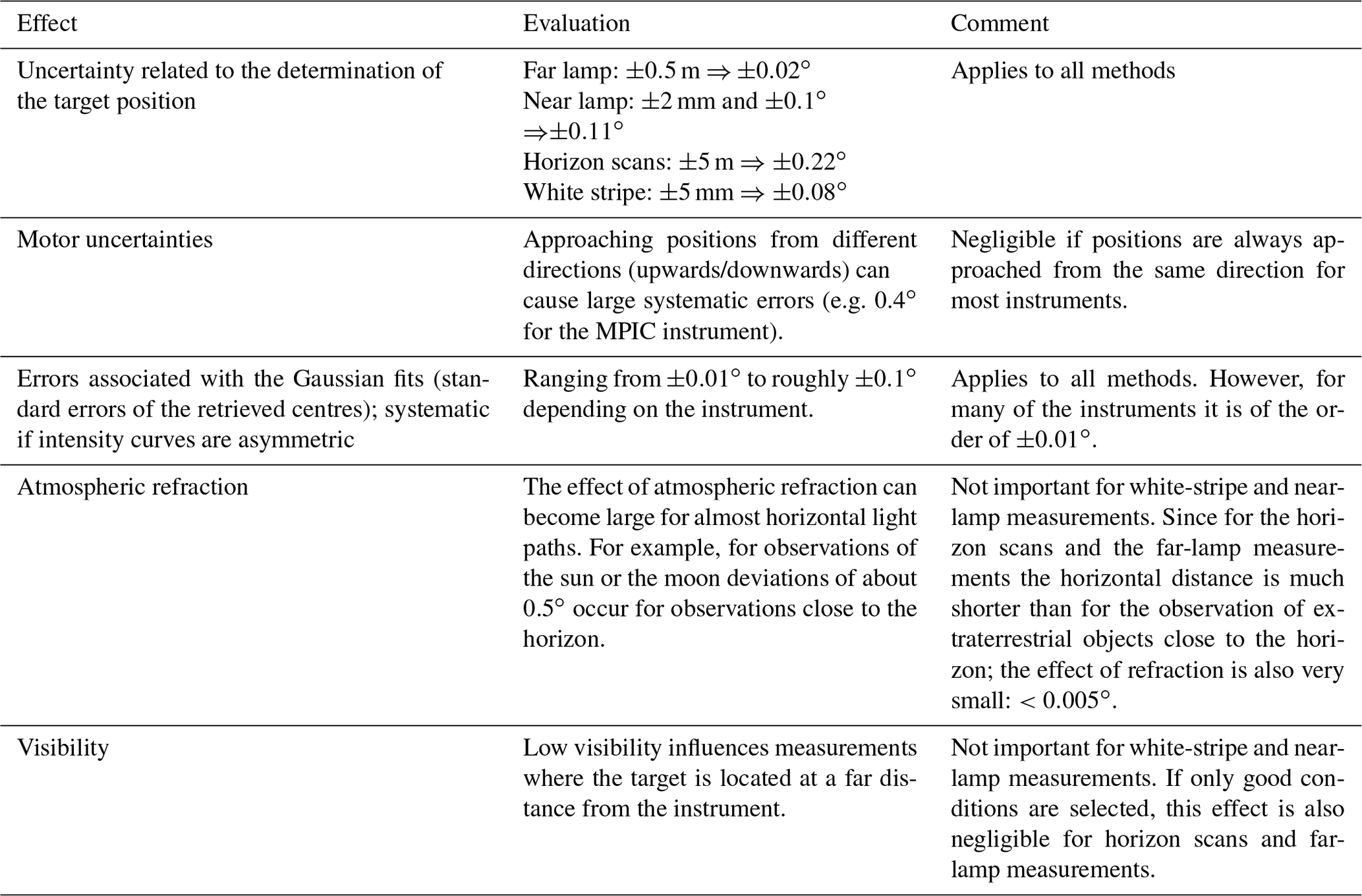
Table A2List and evaluation of statistical effects influencing the measurements presented in this paper.

Data are public available upon request.
All co-authors contributed to the study either as campaign participants or instrument operators; by performing the data analysis and data quality control; or by providing their data of the individual instruments. MVR performed the standardised analysis of the horizon scans. JK, TW and SDO offered and conducted the far-lamp measurements during the campaign. Further, they performed the white-stripe scans. UF and JLT performed and analysed the near-lamp measurements. SDO and TW interpreted the results of the study and wrote the article with feedback and contributions from the other co-authors. TW, SB and SDÖ contributed with valuable feedback and supervised the study.
The authors declare that they have no conflict of interest.
Funding for this study was provided by ESA through the CINDI-2 (ESA Contract no. 4000118533/16/I-Sbo) and FRM4DOAS (FRM4DOAS: ESA Contract No. 4000118181/16/I-EF) projects and partly within the EU 7 Framework Programme QA4ECV (grant agreement no. 607405) project. The BOKU MAX-DOAS instrument was funded and the participation of Stefan F. Schreier was supported by the Austrian Science Fund (FWF): I 2296-N29. The participation of the University of Toronto team was supported by the Canadian Space Agency (through the AVATARS project) and the Natural Sciences and Engineering Research Council (through the PAHA project). The instrument was funded by the Canada Foundation for Innovation and is usually operated at the Polar Environment Atmospheric Research Laboratory (PEARL) by the Canadian Network for the Detection of Atmospheric Change (CANDAC).
The article processing charges for this open-access publication were covered by the Max Planck Society.
This paper was edited by Lok Lamsal and reviewed by three anonymous referees.
Apituley, A. et al.: Second Cabauw Intercomparison of Nitrogen Dioxide Measuring Instruments (CINDI-2) – Campaign Overview, Atmos. Meas. Tech., in preparation, 2020. a, b
Bruchkouski, I., Dziomin, V., and Krasouski, A.: Seasonal variability of the atmospheric trace constituents in Antarctica, 35th Canadian Symposium of Remote Sensing (IGARSS-2014), https://doi.org/10.1109/IGARSS.2014.6947387, 2014. a
Cantrell, C. A.: Technical Note: Review of methods for linear least-squares fitting of data and application to atmospheric chemistry problems, Atmos. Chem. Phys., 8, 5477–5487, https://doi.org/10.5194/acp-8-5477-2008, 2008. a
Clémer, K., Van Roozendael, M., Fayt, C., Hendrick, F., Hermans, C., Pinardi, G., Spurr, R., Wang, P., and De Mazière, M.: Multiple wavelength retrieval of tropospheric aerosol optical properties from MAXDOAS measurements in Beijing, Atmos. Meas. Tech., 3, 863–878, https://doi.org/10.5194/amt-3-863-2010, 2010. a, b
Donner, S.: Mobile MAX-DOAS measurements of the tropospheric formaldehyde column in the Rhein-Main region, Master's thesis, University of Mainz, Mainz, available at: http://hdl.handle.net/11858/00-001M-0000-002C-EB17-2 (last access: 31 January 2020), 2016. a
Drosoglou, T., Bais, A. F., Zyrichidou, I., Kouremeti, N., Poupkou, A., Liora, N., Giannaros, C., Koukouli, M. E., Balis, D., and Melas, D.: Comparisons of ground-based tropospheric NO2 MAX-DOAS measurements to satellite observations with the aid of an air quality model over the Thessaloniki area, Greece, Atmos. Chem. Phys., 17, 5829–5849, https://doi.org/10.5194/acp-17-5829-2017, 2017. a
Fraser, A., Adams, C., Drummond, J. R., Goutail, F., Manney, G., and Strong, K.: “The Polar Environment Atmospheric Research Laboratory UV-visible Ground-Based Spectrometer: First measurements of O3, NO2, BrO, and OClO columns”, J. Quant. Spectrosc. Ra., 110, 986–1004, https://doi.org/10.1016/j.jqsrt.2009.02.034, 2009. a
Frieß, U., Monks, P., Remedios, J., Rozanov, A., Sinreich, R., Wagner, T., and Platt, U.: MAX-DOAS O4 measurements: A new technique to derive information on atmospheric aerosols: 2. Modeling studies, J. Geophys. Res.-Atmos., 111, https://doi.org/10.1029/2005JD006618, 2006. a
Frieß, U., Klein Baltink, H., Beirle, S., Clémer, K., Hendrick, F., Henzing, B., Irie, H., de Leeuw, G., Li, A., Moerman, M. M., van Roozendael, M., Shaiganfar, R., Wagner, T., Wang, Y., Xie, P., Yilmaz, S., and Zieger, P.: Intercomparison of aerosol extinction profiles retrieved from MAX-DOAS measurements, Atmos. Meas. Tech., 9, 3205–3222, https://doi.org/10.5194/amt-9-3205-2016, 2016. a
Hönninger, G. and Platt, U.: Observations of BrO and its vertical distribution during surface ozone depletion at Alert, Atmos. Environ., 36, 2481–2489, 2002. a
Hönninger, G., von Friedeburg, C., and Platt, U.: Multi axis differential optical absorption spectroscopy (MAX-DOAS), Atmos. Chem. Phys., 4, 231–254, https://doi.org/10.5194/acp-4-231-2004, 2004. a, b, c
Irie, H., Kanaya, Y., Akimoto, H., Iwabuchi, H., Shimizu, A., and Aoki, K.: First retrieval of tropospheric aerosol profiles using MAX-DOAS and comparison with lidar and sky radiometer measurements, Atmos. Chem. Phys., 8, 341–350, https://doi.org/10.5194/acp-8-341-2008, 2008. a, b
Kreher, K., Van Roozendael, M., Hendrick, F., Apituley, A., Dimitropoulou, E., Frieß, U., Richter, A., Wagner, T., Abuhassan, N., Ang, L., Anguas, M., Bais, A., Benavent, N., Bösch, T., Bognar, K., Borovski, A., Bruchkouski, I., Cede, A., Chan, K. L., Donner, S., Drosoglou, T., Fayt, C., Finkenzeller, H., Garcia-Nieto, D., Gielen, C., Gómez-Martín, L., Hao, N., Herman, J. R., Hermans, C., Hoque, S., Irie, H., Jin, J., Johnston, P., Khayyam Butt, J., Khokhar, F., Koenig, T. K., Kuhn, J., Kumar, V., Lampel, J., Liu, C., Ma, J., Merlaud, A., Mishra, A. K., Müller, M., Navarro-Comas, M., Ostendorf, M., Pazmino, A., Peters, E., Pinardi, G., Pinharanda, M., Piters, A., Platt, U., Postylyakov, O., Prados-Roman, C., Puentedura, O., Querel, R., Saiz-Lopez, A., Schönhardt, A., Schreier, S. F., Seyler, A., Sinha, V., Spinei, E., Strong, K., Tack, F., Tian, X., Tiefengraber, M., Tirpitz, J.-L., van Gent, J., Volkamer, R., Vrekoussis, M., Wang, S., Wang, Z., Wenig, M., Wittrock, F., Xie, P. H., Xu, J., Yela, M., Zhang, C., and Zhao, X.: Intercomparison of NO2, O4, O3 and HCHO slant column measurements by MAX-DOAS and zenith-sky UV-Visible spectrometers during the CINDI-2 campaign, Atmos. Meas. Tech. Discuss., https://doi.org/10.5194/amt-2019-157, in review, 2019. a, b, c, d, e
Lampel, J., Frieß, U., and Platt, U.: The impact of vibrational Raman scattering of air on DOAS measurements of atmospheric trace gases, Atmos. Meas. Tech., 8, 3767–3787, https://doi.org/10.5194/amt-8-3767-2015, 2015. a, b
Peters, E., Wittrock, F., Großmann, K., Frieß, U., Richter, A., and Burrows, J. P.: Formaldehyde and nitrogen dioxide over the remote western Pacific Ocean: SCIAMACHY and GOME-2 validation using ship-based MAX-DOAS observations, Atmos. Chem. Phys., 12, 11179–11197, https://doi.org/10.5194/acp-12-11179-2012, 2012. a
Pinardi, G., Van Roozendael, M., Abuhassan, N., Adams, C., Cede, A., Clémer, K., Fayt, C., Frieß, U., Gil, M., Herman, J., Hermans, C., Hendrick, F., Irie, H., Merlaud, A., Navarro Comas, M., Peters, E., Piters, A. J. M., Puentedura, O., Richter, A., Schönhardt, A., Shaiganfar, R., Spinei, E., Strong, K., Takashima, H., Vrekoussis, M., Wagner, T., Wittrock, F., and Yilmaz, S.: MAX-DOAS formaldehyde slant column measurements during CINDI: intercomparison and analysis improvement, Atmos. Meas. Tech., 6, 167–185, https://doi.org/10.5194/amt-6-167-2013, 2013. a
Piters, A. J. M., Boersma, K. F., Kroon, M., Hains, J. C., Van Roozendael, M., Wittrock, F., Abuhassan, N., Adams, C., Akrami, M., Allaart, M. A. F., Apituley, A., Beirle, S., Bergwerff, J. B., Berkhout, A. J. C., Brunner, D., Cede, A., Chong, J., Clémer, K., Fayt, C., Frieß, U., Gast, L. F. L., Gil-Ojeda, M., Goutail, F., Graves, R., Griesfeller, A., Großmann, K., Hemerijckx, G., Hendrick, F., Henzing, B., Herman, J., Hermans, C., Hoexum, M., van der Hoff, G. R., Irie, H., Johnston, P. V., Kanaya, Y., Kim, Y. J., Klein Baltink, H., Kreher, K., de Leeuw, G., Leigh, R., Merlaud, A., Moerman, M. M., Monks, P. S., Mount, G. H., Navarro-Comas, M., Oetjen, H., Pazmino, A., Perez-Camacho, M., Peters, E., du Piesanie, A., Pinardi, G., Puentedura, O., Richter, A., Roscoe, H. K., Schönhardt, A., Schwarzenbach, B., Shaiganfar, R., Sluis, W., Spinei, E., Stolk, A. P., Strong, K., Swart, D. P. J., Takashima, H., Vlemmix, T., Vrekoussis, M., Wagner, T., Whyte, C., Wilson, K. M., Yela, M., Yilmaz, S., Zieger, P., and Zhou, Y.: The Cabauw Intercomparison campaign for Nitrogen Dioxide measuring Instruments (CINDI): design, execution, and early results, Atmos. Meas. Tech., 5, 457–485, https://doi.org/10.5194/amt-5-457-2012, 2012. a, b
Roscoe, H. K., Van Roozendael, M., Fayt, C., du Piesanie, A., Abuhassan, N., Adams, C., Akrami, M., Cede, A., Chong, J., Clémer, K., Friess, U., Gil Ojeda, M., Goutail, F., Graves, R., Griesfeller, A., Grossmann, K., Hemerijckx, G., Hendrick, F., Herman, J., Hermans, C., Irie, H., Johnston, P. V., Kanaya, Y., Kreher, K., Leigh, R., Merlaud, A., Mount, G. H., Navarro, M., Oetjen, H., Pazmino, A., Perez-Camacho, M., Peters, E., Pinardi, G., Puentedura, O., Richter, A., Schönhardt, A., Shaiganfar, R., Spinei, E., Strong, K., Takashima, H., Vlemmix, T., Vrekoussis, M., Wagner, T., Wittrock, F., Yela, M., Yilmaz, S., Boersma, F., Hains, J., Kroon, M., Piters, A., and Kim, Y. J.: Intercomparison of slant column measurements of NO2 and O4 by MAX-DOAS and zenith-sky UV and visible spectrometers, Atmos. Meas. Tech., 3, 1629–1646, https://doi.org/10.5194/amt-3-1629-2010, 2010. a, b
Schreier, S. F., Richter, A., Peters, E., Ostendorf, M., Schmalwieser, A. W., Weihs, P., and Burrows, J. P.: Dual ground-based MAX-DOAS observations in Vienna, Austria: Evaluation of horizontal and temporal NO2, HCHO, and CHOCHO distributions and comparison with independent data sets, Atmos. Environ., 5, https://doi.org/10.1016/j.aeaoa.2019.100059, 2019. a
Van Roozendael, M., Fayt, C., Post, P., Hermans, C., and Lambert, J. C.: Retrieval of Tropospheric BrO and NO2 from UV-Visible Observations, Springer, Heidelberg, 155–165, https://doi.org/10.1007/978-3-642-18875-6_19, 2004. a
Wagner, T., Dix, B., Friedeburg, C. v., Frieß, U., Sanghavi, S., Sinreich, R., and Platt, U.: MAX-DOAS O4 measurements – a new technique to derive information on atmospheric aerosols, (I) Principles and information content, J. Geophys. Res.-Atmos., 109, D22205, https://doi.org/10.1029/2004JD004904, 2004. a
Wagner, T., Beirle, S., Brauers, T., Deutschmann, T., Frieß, U., Hak, C., Halla, J. D., Heue, K. P., Junkermann, W., Li, X., Platt, U., and Pundt-Gruber, I.: Inversion of tropospheric profiles of aerosol extinction and HCHO and NO2 mixing ratios from MAX-DOAS observations in Milano during the summer of 2003 and comparison with independent data sets, Atmos. Meas. Tech., 4, 2685–2715, https://doi.org/10.5194/amt-4-2685-2011, 2011. a, b
Wittrock, F., Oetjen, H., Richter, A., Fietkau, S., Medeke, T., Rozanov, A., and Burrows, J. P.: MAX-DOAS measurements of atmospheric trace gases in Ny-Ålesund – Radiative transfer studies and their application, Atmos. Chem. Phys., 4, 955–966, https://doi.org/10.5194/acp-4-955-2004, 2004. a
- Abstract
- Introduction
- Campaign overview and MAX-DOAS instruments
- Methods of elevation calibration
- Comparison between different instruments
- Overall discussion and conclusions
- Appendix A: Error assessment
- Data availability
- Author contributions
- Competing interests
- Acknowledgements
- Financial support
- Review statement
- References