the Creative Commons Attribution 4.0 License.
the Creative Commons Attribution 4.0 License.
 | 17 Feb 2020
Quantifying hail size distributions from the sky – application of drone aerial photogrammetry
Joshua S. Soderholm
Matthew R. Kumjian
Nicholas McCarthy
Paula Maldonado
Minzheng Wang
A new technique, named “HailPixel”, is introduced for measuring the maximum dimension and intermediate dimension of hailstones from aerial imagery. The photogrammetry procedure applies a convolutional neural network for robust detection of hailstones against complex backgrounds and an edge detection method for measuring the shape of identified hailstones. This semi-automated technique is capable of measuring many thousands of hailstones within a single survey, which is several orders of magnitude larger (e.g. 10 000 or more hailstones) than population sizes from existing sensors (e.g. a hail pad). Comparison with a co-located hail pad for an Argentinian hailstorm event during the RELAMPAGO project demonstrates the larger population size of the HailPixel survey significantly improves the shape and tails of the observed hail size distribution. When hail fall is sparse, such as during large and giant hail events, the large survey area of this technique is especially advantageous for resolving the hail size distribution.


Measurements of the hail size distribution (HSD) are challenging to collect owing to the infrequent and hostile nature of hailstorms. Because of these constraints, HSD measurements are uncommon, especially for larger hail (>25 mm). Such observations are necessary to constrain hail microphysics parameterization schemes used in weather and climate models and for hail detection and sizing algorithms from weather radar. Improvements to hail retrievals and modelling are an important step towards mitigating the increasingly significant hail-related losses to agriculture, motor vehicles and buildings (Sánchez et al., 1996; Changnon et al., 1997; Hohl et al., 2002).
Ground sensors for measuring the size distribution of large hail can be separated into those that provide time recording (e.g. hail disdrometer) and those that provide time-integrated measurements (e.g. hail pad). Time-recording instruments such as impact or optical disdrometers provide valuable information on the temporal variability of the HSD within a given storm but are often expensive to fabricate and maintain and difficult to deploy. Thus, such instruments typically are only deployed as smaller networks or for field campaigns (e.g. Federer and Waldvogel, 1975; Löffler-Mang et al., 2011; Brown et al., 2014). In contrast, time-integrated instruments often are cheaper to fabricate, maintain and deploy, making them attractive options for longer-term monitoring of hail fall. The most commonly used time-integrated instrument for measuring HSDs is a hail pad, consisting of a foil-covered styrofoam pad that preserves dents of hail impact (Long et al., 1979). This sensor is cost-effective and has seen extensive use by previous and ongoing campaigns in the US and Europe over the last 50 years (Cheng and English, 1983; Fraile et al., 1992; Cifelli et al., 2005; Kalina et al., 2014). Both hail pads and hail disdrometers provide reasonable estimates of hail size but are subject to significant limitations even with careful calibration (e.g. Palencia et al., 2011). Further, both time-recording and time-integrated instruments for measuring the HSD utilize a small sample area on the order of 0.1 to 0.3 m2. Towery et al. (1976) suggest this small sample area is likely to under-represent the HSD, particularly for larger hail, and recommend deployment of multiple sensors to minimize this effect.
The concentration of large hail, and particularly giant hail (>100 mm), can be very sparse (Witt et al., 2018), severely limiting the effectiveness of these small ground sensors even with multiple units. To overcome these sampling limitations, we describe a new time-integrated technique for measuring the HSD by combining aerial imagery captured from a small unmanned aircraft with deep learning and computer vision feature extraction. Methods involving deep learning have seen increased utilization in the atmospheric sciences community, including for the application of severe weather (e.g. McGovern et al., 2017; Gagne et al., 2019); however, there has been limited usage of such methods in targeted field observation datasets and in situ data. Over the last 2 decades, convolutional neural networks (CNNs) have become a rapidly developing deep-learning research tool that excels at image feature recognition (e.g. Razavian et al., 2014; Krizhevsky et al., 2012). This is achieved by developing complex feature recognition filters independent of prior knowledge, inspired by processes within the animal visual cortex (Hubel and Wiesel, 1968).
The new technique described here, named “HailPixel”, enables the capture of very large areas (>1500 m2, equivalent area to several thousand hail pads) immediately following a hailstorm. This paper describes the methods of imagery capture and semi-automated extraction of the HSD using a combination of CNNs and computer vision techniques. Results from a HailPixel survey of a hailstorm on 26 November 2018 in San Rafael (Argentina) are discussed in the context of existing studies and potential improvements for future surveys.
To effectively extract the HSD from aerial imagery, the hailstone size must be significantly larger than the effective ground resolution of the sensor, and the concentration of hailstones must be sufficiently low so that overlapping stones are minimized. Aerial-imagery surveys of hail coverage were conducted in the Mendoza Province of Argentina after hailstorms on 25 and 26 November 2018 during the RELAMPAGO field campaign (Nesbitt et al., 2018). Only the 26 November event produced non-accumulating hail of sufficiently large diameters (>20 mm), and imagery from this event will be used throughout the paper. The hail swath observed from the 26 November event was produced by a marginally supercellular storm that developed in an environment of moderate instability and deep-layer shear. The storm started in the Andes and tracked approximately 120 km east-northeast towards the city of San Rafael before observations were made. A single hail pad (300 mm × 400 mm × 30 mm polystyrene foam block covered in aluminium foil) was also deployed 2 km southwest of the aerial-survey site for the San Rafael hailstorm (34.6533∘ S, 68.5030∘ W), providing a secondary measure of the HSD. To estimate hail size from hail pad indentations, the major- and minor-axis lengths of individual dents were measured with digital calipers and transformed into hail major- and minor-axis size using a relationship developed by the Community Collaborative Rain, Hail and Snow Network (Nolan Doesken, personal communication, 17 April 2019).
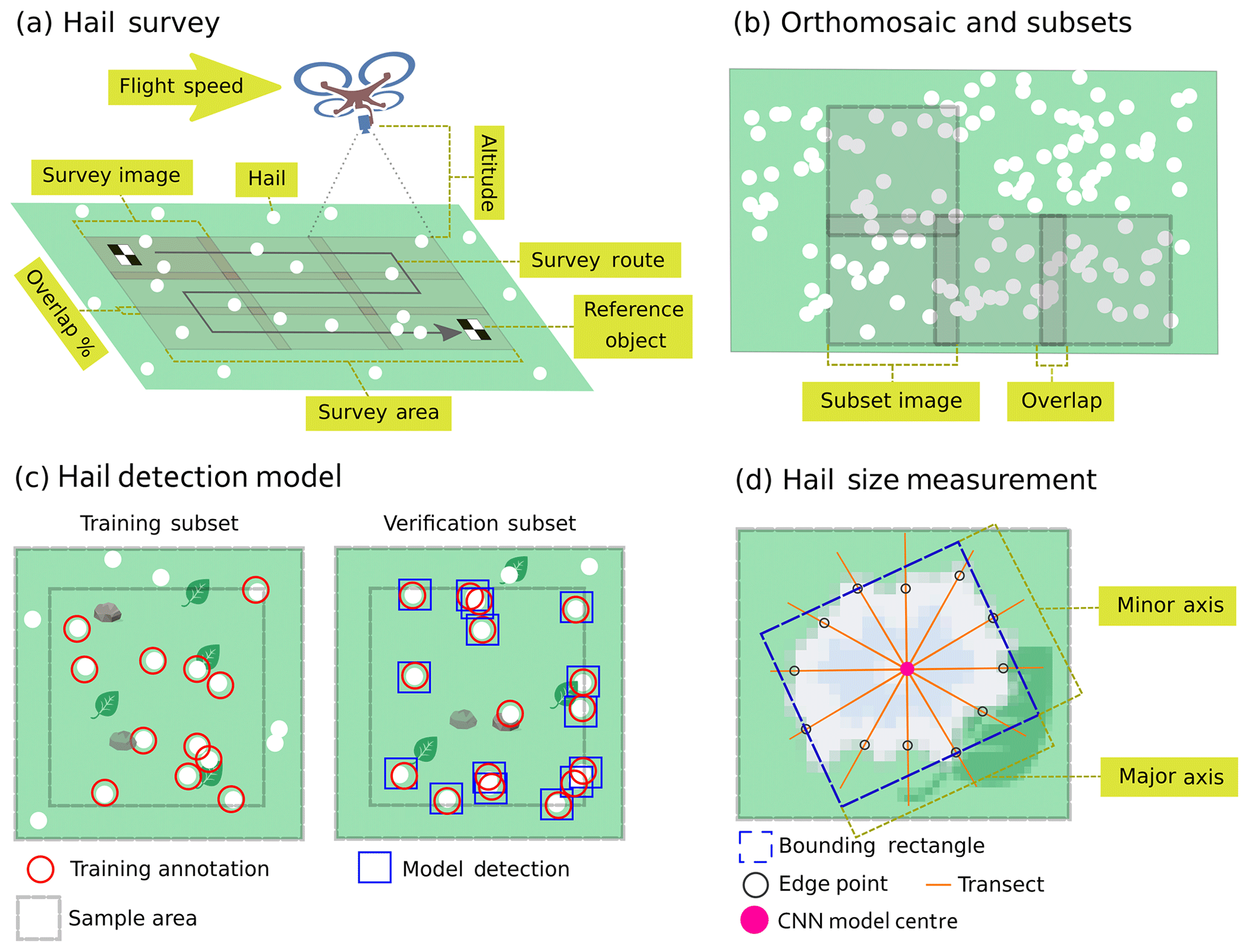
Figure 1Workflow of (a) data collection, (b) tiling of orthomosaic, (c) hail detection using the Mask R-CNN technique and (d) hail size measurement using radial transects.
2.1 Imagery
A DJI Phantom 4 Pro V2 aircraft and Pix4Dcapture flight-control software were used for image acquisition. The integrated, gimbal-mounted aircraft camera uses a 13.2 mm × 8.8 mm active-pixel sensor which provides 20M effective pixels, automatic exposure, and an autofocus lens with a focal length of 8.8–24 mm and maximum field of view of 84∘. For the 26 November event, the aircraft was flown at an altitude of 10 m (relative to the take-off location) over a rectangular survey area of 1290 m2 centred on 34.6459∘ S, 68.4814∘ W, providing a ∼2.7 mm ground sampling distance (Fig. 1a). Near-surface wind speed at the time of capture was noted by the authors to be a gentle breeze (3.5–5.5 ms−1), reducing the likelihood of wind-induced motion blur. Images were captured with a 70 % overlap laterally and medially at a flight speed of 1 m s−1 over a surface consisting of sparse grasses, small shrubs, gravel and dirt. A large image overlap and slow flight speed were selected to increase the number of quality matching points during orthomosaic construction and reduce motion blur (Bemis et al., 2014). The survey was initialized immediately once hail fall concluded and required approximately 4 min to complete. The location of images was measured using the integrated GPS receiver, which has an accuracy of ±1.5 m. Precise location measurements (e.g. real-time kinematic positioning) are not essential for improving the pixel size accuracy during photogrammetry processing (Küng, 2012).
The Pix4Dmapper software package was used to generate orthomosaic imagery and a digital elevation model (DEM) from the survey photos (Küng, 2012) with a ground sampling distance of 2.7 mm. The software is based on the structure-from-motion photogrammetry technique and uses the following automated steps:
-
Tie points between the survey images are identified. Each tie point must be matched in at least three images.
-
Tie points are combined with positioning and orientation information from the aircraft autopilot to reconstruct the camera perspective and position for each survey image. This information is used to verify the quality of matching points and calculate the 3-D coordinates of tie points.
-
The sparse point cloud of 3-D coordinates is interpolated to obtain a gridded DEM.
-
The DEM is used to project every image pixel and to calculate an orthomosaic.
An average of 181 081 matched tie points were found per cubic metre with a mean geolocation error of less than 1 mm. Analysis of the DEM indicates a gradual slope was present across the survey area with a total change in elevation of approximately 2.3 m (not shown). Two scale markers consisting of 300 mm × 300 mm black and white vinyl tiles were also placed into the aerial-survey area to provide a secondary check of pixel size within the orthomosaic.
2.2 Hail detection
To efficiently identify the many thousands of hailstones captured in the aerial imagery after the San Rafael hailstorm, automated feature detection techniques were explored. Simple thresholding of pixel luminosity for detecting hailstones performed poorly owing to similar luminosity from sparse grasses, light dirt patches, pale-coloured rocks and leaf debris and to instances when hailstones were in contact. Despite the low contrast, hailstones were easily identifiable in the imagery by human observers, motivating the application of the state-of-the-art Mask regional CNN (R-CNN) model (He et al., 2017). This technique combines the optimized selection and parallel processing of proposed feature regions (Fast R-CNN) with semantic segmentation, whereby each pixel is classified. Mask R-CCN architecture and implementation methods used are described in detail by He et al. (2017).

Figure 2Demonstration of hail size extraction from the 26 November 2018 survey orthomosaic (a) from a single tile (b: blue bounding box) for a single hailstone (c: black circle in b). Radial transects for extracting imagery lightness are shown in (c) as black lines radiating from hailstone centroid (blue marker), and hailstone edge pixels along transects are numbered. The subplot in panel (d) shows the normalized pixel lightness along the 12 transects shown in (c) with the corresponding edge pixels marked.
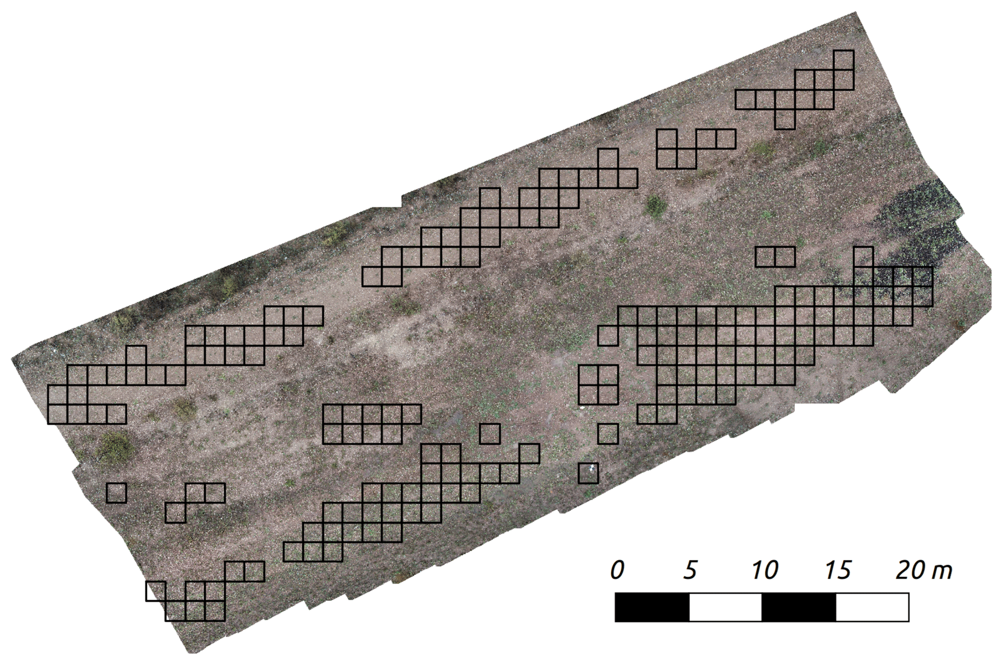
Figure 3Orthomosaic RGB imagery from the 26 November 2018 survey overlaid with the outlines of tiles used for the extraction of hail size distribution statistics.
To reduce memory requirements, the 489 MP aerial-survey orthomosaic was divided into 1961 tiles of size 600 pixels × 600 pixels, including a 50-pixel overlap along edges with neighbouring tiles to avoid cropped hailstones (Figs. 1b, 2a, b). To provide a sufficiently large sample of hailstones for training the Mask R-CNN model, 12 tiles were manually selected that in total contained more than 1000 stones and were annotated using the VGG Image Annotator (VIA) tool (Dutta and Zisserman, 2019). These tiles were also selected to sample the varying background types across the orthomosaic. Nine tiles were randomly selected for training (containing 729 annotated hailstones) and the remaining three for validation (Fig. 1c). The Mask R-CNN training was initialized with the pre-trained weights from the Microsoft COCO dataset (set of labelled images; Lin et al., 2014), which capture many features in natural images. Utilizing these weights greatly reduces the training time required to recognize hail. The default learning and weighting configuration described by He et al. (2017) was applied, and training was performed on eight GPUs with one image per GPU for 3000 iterations (∼43 min of computation time). The trained model detected more than 94 % of the hailstones in each validation tile with a false-alarm rate of <1 %. When applied to all tiles, the trained Mask R-CNN model detected a total of 46 871 hailstones.
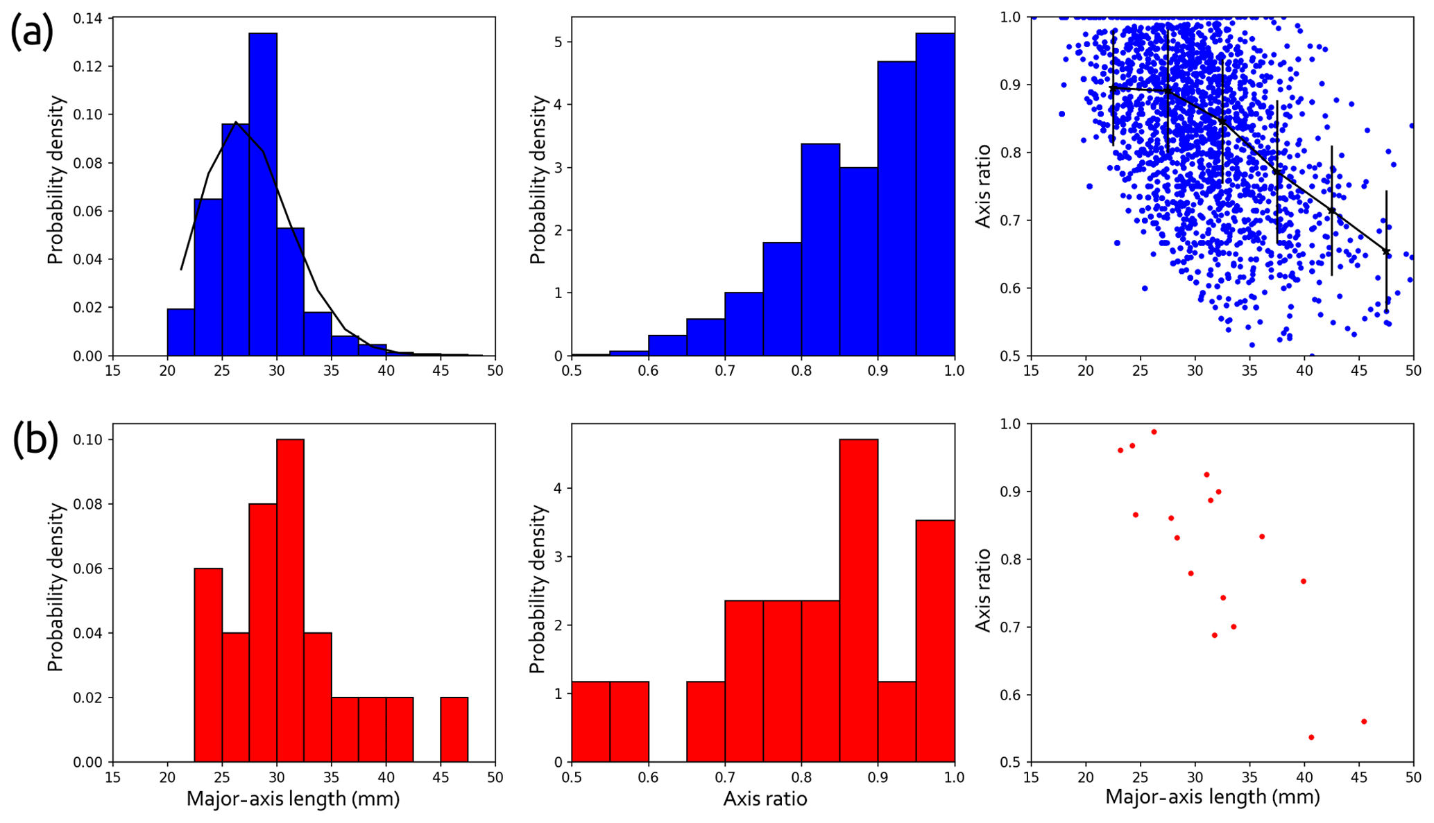
Figure 4Distribution of hail major-axis length, minor-axis ratio, and scatter plot of axis ratio and major-axis length from the (a) photogrammetry and (b) pad hail size retrievals for the 26 November 2018 survey. A fitted gamma distribution probability density function for the photogrammetry major-axis size distribution is shown (black line). Photogrammetry scatter plot observations are binned using 5 mm bin sizes and error bars represent ±1 standard deviation.
2.3 Hail size measurement
The segmentation mask generated by the Mask R-CNN model was initially tested for hail size measurement but was found to contain small errors that rendered it unsuitable. To provide the pixel-level accuracy required for measuring hailstones, an edge detection algorithm was developed to find the steep lightness gradient1 at the hailstone edge that occurs radially from the hailstone centroid (Fig. 1d). The HSL colour space is an alternative to the red–green–blue model (RGB; developed for colour displays) that is commonly used in computer vision applications for reducing the correlation between colours (Cheng et al., 2001). The hailstone centroids required to initialize the edge detection technique are derived from the segmentation mask. Two additional quality control steps are also applied to the centroids and image tiles:
-
Tiles where hail was obscured (e.g. under long grass or shrubs) or water had accumulated were removed, leaving 188 clean image tiles containing 15 983 hailstones over a total area of 342.6 m2 for hail size measurement.
-
Hail centroids for the 188 clean image tiles were manually assessed and amended if required using the VIA annotation tool.
The clean image tiles are next transformed into the HSL colour space and the hailstone size is measured for every centroid using the following procedure. First, coordinates of 12 equally spaced radials of length 20 pixels from the centroid (p0) are calculated (Fig. 2c), denoted as , where i is the pixel index () and k is the radial index (). For all points along a radial, the lightness values are extracted. Then, the gradient of lightness values along each radial are calculated. Starting from the centroid of each radial, the edge point is found at coordinate when the following criteria are met:
and
The required minimum lightness difference between the hailstone centroid and background (50) was found to perform well across all background types, including light-coloured soils. Once all edge points are found along the radials (Fig. 2d), the median distance from the centroid is calculated for each edge point. If an edge point falls outside the range to , it is replaced by . Finally, to measure the major- and minor-axis length of the hailstone, the minimum bounding box (allowing for rotation) is calculated for the set of edge points.
The resulting distribution of major-axis length and axis ratio for the San Rafael hailstorm is shown in Fig. 4, along with the distributions obtained from the hail pad (total of 17 impacts). A comparison of the major-axis length distribution from the HailPixel and hail pad techniques clearly demonstrates the value of aerial photogrammetry: the large population size (n=15 983) of the aerial survey provides a defined distribution shape and tails (Fig. 4). The HailPixel distribution peak is 2.5 mm lower than the hail pad peak, possibly due to melting of hail on the ground before it was photographed or uncertainty in hail size retrievals. The distribution shape is well approximated by a gamma probability distribution function (PDF) with a mostly absent lower quartile and long upper tail. The gamma PDF was also found to be most suited to major-axis length in a number of other case studies, including Ziegler et al. (1983) for Oklahoma (US), Wong et al. (1988) for Alberta (Canada) and Fraile et al. (1992) for León (Spain). Impact concentration observed by the hail pad was 141 m−2, significantly higher than the mean hail concentration observed by the aerial survey (47 m−2). This difference is speculated to be the product of longer hail fall duration at the hail pad location (2 km southwest) and possible secondary impacts on the hail pad from bouncing stones.
The distribution of axis ratios from the HailPixel survey is well approximated by an exponentially increasing function (not shown); however, a local maximum at 0.8–0.85 suggests a more complex underlying distribution. Note that oblate hailstones are most likely to rest on the surface with their minor axis orientated vertically; thus, the HailPixel technique would not measure the true minor-axis length in this scenario but rather provide estimates of the intermediate-axis ratio (assuming ellipsoidal geometry for hailstones). This limitation is likely to also affect hail pad measurements when tumbling motions of oblate hailstones are not too extreme. Comparing the HailPixel intermediate- and major-axis distribution with Giammanco et al. (2014) major- and minor-axis distributions demonstrates the expected skew towards higher axis ratios in the HailPixel dataset.
Both HailPixel and hail pad data demonstrate a decreasing axis ratio with increasing hail size. This shape of the relationship becomes apparent when the highly variable HailPixel data are binned into 5 mm intervals. For the 20–30 mm hail size range, the axis ratio remains constant and close to 0.9. For sizes >30 mm, the axis ratio decreases by 0.4–0.5 % mm−1. Despite the potential bias in axis ratio measurements, the shape of this trend is comparable to observations by Knight (1986) for an Alberta (Canada) hailstorm. Another study using a 3-year database of hailstones collected from the Great Plains by Giammanco et al. (2014) demonstrates a less significant decreasing trend between hail size and axis ratio and less spherical stones for smaller sizes. It is likely that this relationship is also highly variable between hailstorm cases and within hailstorms (Federer and Waldvogel, 1975; Ziegler et al., 1983; Knight, 1986).
It is also important to highlight the optimal conditions and configuration for future HailPixel surveys. We recommend avoiding inhomogeneous background surfaces if possible, with cut or grazed turf grasses being most ideal. A uniform and contrasting background will likely permit the use of less complex hail detection and sizing techniques. Large survey areas (>1000 m2) are only necessary when very sparse giant (>100 mm) hailstones are present. Assuming a normally distributed sample mean, a sample size of 2088 hailstones is required to represent the population mean (from 15 983 hailstones) within a 2 % confidence level at the 95 % significance level. This sample size equates to a sample area of 40.1 m2 for the 26 November survey; however, an area of at least ∼250 m2 is recommended to adequately resolve the tails of the distribution. For the DJI Phantom 4 Pro V2 aircraft flown at a 10 m altitude, the authors recommend a minimum hail diameter of 20 mm (major-axis length) and less than 30 % total ground coverage. The minimum size limit is particularly critical when separating multiple stones in contact. Higher-resolution imagery would allow for small (<20 mm) hailstones to be measured, but the increased susceptibility to motion blur would likely require the aircraft to remain stationary during image capture. Further, 10 m winds exceeding a moderate breeze (>8 ms1) would increase the likelihood of motion blur. To quantify the measurement uncertainty from the HailPixel technique, we recommend that hail within a 1 m2 area of the aerial survey is manually measured for three orthogonal axes immediately following aerial capture. Finally, minimizing the melting of hailstones is critical. Where possible, avoid aerial surveys of areas where water may flow or accumulate, and conduct surveys immediately after hail fall ceases.
This paper describes the novel HailPixel aerial photogrammetry technique for measuring time-integrated HSDs after the cessation of hail fall. The workflow for collecting imagery, detecting hailstones and measuring hail size is described, including the use of the state-of-the-art Mask R-CNN image segmentation algorithm. Results from a HailPixel survey after the 26 November 2018 San Rafael (Argentina) hailstorm are compared with observations from a co-located hail pad. Despite a potential bias in axis ratio measurements, the HSD and relationships observed for the San Rafael hailstorm are comparable to previous studies. In contrast to hail impact sensors, the use of aerial imagery provided a sample area that is several orders of magnitude larger (341.6 m2). As a result, the hailstone population size from the 26 November 2018 imagery was substantially larger than previous studies (15 983 hailstones), providing a more robust analysis of the HSD. Ongoing work to relate HailPixel results with mobile polarimetric radar observations from the 26 November 2018 San Rafael hailstorm will explore the signatures of hail size and swath extent for this event. Future HailPixel surveys are encouraged to quantify the variability of these distributions, particularly for hailstorms producing sparse giant hail.
All imagery and hail pad and hail retrieval data used for this work are publicly available: Soderholm (2019) (https://doi.org/10.5281/zenodo.3383227).
JSS designed the HailPixel technique, and JSS, MRK, NM and PM applied the technique following hailstorms during the RELAMPAGO project. JSS developed the hail identification and sizing algorithms with assistance from MW. JSS prepared the manuscript with contributions from all co-authors.
The authors declare that they have no conflict of interest.
The authors wish to thank the RELAMPAGO project for the unique opportunity to operate HailPixel surveys in Argentina. Initial testing, methodology reviews and equipment loans were provided by the School of Earth, Atmosphere and Environment, Monash University, in particular by Sam Thiele and Steven Micklethwaite.
This research has been supported by the Australian National Environmental Science Program; Amazon Web Services (Earth on AWS through the AWS Cloud Credits for Research programme); the Alexander von Humboldt Foundation; the National Science Foundation, Division of Atmospheric and Geospace Sciences (grant no. AGS-1661679); and the Insurance Institute for Business and Home Safety.
This paper was edited by Brian Kahn and reviewed by Tomeu Rigo and two anonymous referees.
Bemis, S. P., Micklethwaite, S., Turner, D., James, M. R., Akciz, S., Thiele, S. T., and Bangash, H. A.: Ground-based and UAV-Based photogrammetry: A multi-scale, high-resolution mapping tool for structural geology and paleoseismology, J. Struct. Geol., 69, 163–178, https://doi.org/10.1016/j.jsg.2014.10.007, 2014. a
Brown, T. M., Giammanco, I. M., and Kumjian, M. R.: IBHS Hail Field Research Program: 2012–2014, in: 27th Conference on Severe Local Storms, November, 2012–2014, American Meteorological Society, Madison, WI, 2014. a
Changnon, S. A., Changnon, D., Ray Fosse, E., Hoganson, D. C., Roth, R. J., and Totsch, J. M.: Effects of Recent Weather Extremes on the Insurance Industry: Major Implications for the Atmospheric Sciences, B. Am. Meteorol. Soc., 78, 425–435, https://doi.org/10.1175/1520-0477(1997)078<0425:EORWEO>2.0.CO;2, 1997. a
Cheng, H., Jiang, X., Sun, Y., and Wang, J.: Color image segmentation: advances and prospects, Pattern Recogn., 34, 2259–2281, https://doi.org/10.3346/jkms.2018.33.e6, 2001. a
Cheng, L. and English, M.: A Relationship Between Hailstone Concentration and Size, J. Atmos. Sci., 40, 204–213, https://doi.org/10.1175/1520-0469(1983)040<0204:arbhca>2.0.co;2, 1983. a
Cifelli, R., Doesken, N., Kennedy, P., Carey, L. D., Rutledge, S. A., Gimmestad, C., and Depue, T.: The Community Collaborative rain, hail, and snow network, B. Am. Meteorol. Soc., 86, 1069–1077, https://doi.org/10.1175/BAMS-86-8-1069, 2005. a
Dutta, A. and Zisserman, A.: The {VIA} Annotation Software for Images, Audio and Video, arXiv preprint arXiv:1904.10699, https://doi.org/10.1145/3343031.3350535, 2019. a
Federer, B. and Waldvogel, A.: Hail and Raindrop Size Distributions from a Swiss Multicell Storm, J. Appl. Meteorol., 14, 91–97, https://doi.org/10.1175/1520-0450(1975)014<0091:harsdf>2.0.co;2, 1975. a, b
Fraile, R., Castro, A., and Sánchez, J. L.: Analysis of hailstone size distributions from a hailpad network, Atmos. Res., 28, 311–326, https://doi.org/10.1016/0169-8095(92)90015-3, 1992. a, b
Gagne, D. J., Haupt, S. E., Nychka, D. W., and Thompson, G.: Interpretable Deep Learning for Spatial Analysis of Severe Hailstorms, Mon. Weather Rev., 147, 2827–2845, https://doi.org/10.1175/MWR-D-18-0316.1, 2019. a
Giammanco, I. M., Kumjian, M. R., and Heymsfield, A. J.: Observations of Hailstone Sizes and Shapes from the IBHS Hail Measurement Program: 2012–2014, in: 27th Conference on Severe Local Storms, December, 1–9, American Meteorological Society, Madison, WI, 2014. a, b
He, K., Gkioxari, G., Dollar, P., and Girshick, R.: Mask R-CNN, Proceedings of the IEEE International Conference on Computer Vision, October, 2980–2988, https://doi.org/10.1109/ICCV.2017.322, 2017. a, b, c
Hohl, R., Schiesser, H. H., and Aller, D.: Hailfall: The relationship between radar-derived hail kinetic energy and hail damage to buildings, Atmos. Res., 63, 177–207, https://doi.org/10.1016/S0169-8095(02)00059-5, 2002. a
Hubel, D. H. and Wiesel, T. N.: Receptive Fields and Functional Architecture of Monkey Striate Cortex, J. Physiol., 195, 215–243, https://doi.org/10.1113/jphysiol.1968.sp008455, 1968. a
Kalina, E. A., Friedrich, K., Ellis, S. M., and Burgess, D. W.: Comparison of Disdrometer and X-Band Mobile Radar Observations in Convective Precipitation, Mon. Weather Rev., 142, 2414–2435, https://doi.org/10.1175/mwr-d-14-00039.1, 2014. a
Knight, N. C.: Hailstone Shape Factor and Its Relation to Radar Interpretation of Hail, J. Clim. Appl. Meteorol., 25, 1956–1958, https://doi.org/10.1175/1520-0450(1986)025<1956:hsfair>2.0.co;2, 1986. a, b
Krizhevsky, A., Sutskever, I., and Hinton, G. E.: ImageNet Classification with Deep Convolutional Neural Networks, Commun. ACM, 60, 84–90, https://doi.org/10.1201/9781420010749, 2012. a
Küng, O., Strecha, C., Beyeler, A., Zufferey, J.-C., Floreano, D., Fua, P., and Gervaix, F.: THE ACCURACY OF AUTOMATIC PHOTOGRAMMETRIC TECHNIQUES ON ULTRA-LIGHT UAV IMAGERY, Int. Arch. Photogramm. Remote Sens. Spatial Inf. Sci., XXXVIII-1/C22, 125–130, https://doi.org/10.5194/isprsarchives-XXXVIII-1-C22-125-2011, 2011. a, b
Lin, T. Y., Maire, M., Belongie, S., Hays, J., Perona, P., Ramanan, D., Dollár, P., and Zitnick, C. L.: Microsoft COCO: Common objects in context, Lecture Notes in Computer Science, 8693 LNCS, 740–755, https://doi.org/10.1007/978-3-319-10602-1_48, 2014. a
Löffler-Mang, M., Schön, D., and Landry, M.: Characteristics of a new automatic hail recorder, Atmos. Res., 100, 439–446, https://doi.org/10.1016/j.atmosres.2010.10.026, 2011. a
Long, A. B., Matson, R. J., and Crow, E. L.: The Hailpad: Materials, Data Reduction and Calibration, J. Appl. Meteorol., 19, 1300–1313, https://doi.org/10.1175/1520-0450(1980)019<1300:thmdra>2.0.co;2, 1979. a
McGovern, A., Elmore, K. L., Gagne, D. J., Haupt, S. E., Karstens, C. D., Lagerquist, R., Smith, T., and Williams, J. K.: Using Artificial Intelligence to Improve Real-Time Decision-Making for High-Impact Weather, B. Am. Meteorol. Soc., 98, 2073–2090, https://doi.org/10.1175/BAMS-D-16-0123.1, 2017. a
Nesbitt S. W., Salio P., Trapp R. J., Roberts R. D., Varble A. C., Dominguez F., Machado L. A. T., and Saulo C.: Understanding Processes and Improving Predictions of Hydrometeorological Extremes in Subtropical South America: Proyecto RELAMPAGO-CACTI, 32nd Conference on Hydrology, Austin, Texas, 9 January 2018, 6.3, 2018. a
Palencia, C., Castro, A., Giaiotti, D., Stel, F., and Fraile, R.: Dent overlap in hailpads: Error estimation and measurement correction, J. Appl. Meteorol. Clim., 50, 1073–1087, https://doi.org/10.1175/2010JAMC2457.1, 2011. a
Razavian, A. S., Hossein, A., Josephine, S., and Stefan, C.: CNN features off-the-Shelf: An astounding baseline for recognition, CoRR, 806–813, https://doi.org/10.1109/cvprw.2014.131, 2014. a
Sánchez, J. L., Fraile R., de la Madrid J. L., de la Fuente M. T., Rodríguez P., and Castro A.: Crop Damage: The Hail Size Factor, J. Appl. Meteorol., 35, 1535–1541, https://doi.org/10.1175/1520-0450(1996)035<1535:CDTHSF>2.0.CO;2, 1996. a
Soderholm, J. S.: HailPixel Survey Data and Analysis from 26 November 2018, San Rafael, Argentina [Data set], Zenodo, https://doi.org/10.5281/zenodo.3383227, 2019. a
Towery, N. G., Changnon, S. A., and Morgan, G. M.: A Review of Hail-Measuring Instruments, B. Am. Meteorol. Soc., 57, 1132–1140, https://doi.org/10.1175/1520-0477(1976)057<1132:AROHMI>2.0.CO;2, 1976. a
Witt, A., Burgess, D. W., Seimon, A., Allen, J. T., Snyder, J. C., and Bluestein, H. B.: Rapid-Scan Radar Observations of an Oklahoma Tornadic Hailstorm Producing Giant Hail, Weather Forecast., 33, 1263–1282, https://doi.org/10.1175/WAF-D-18-0003.1, 2018. a
Wong, R. K. W., Chidambaram, N., Lawrence, C., and English, M.: The Sampling Variations of Hailstone Size Distributions, J. Appl. Meteorol., 27, 254–260, https://doi.org/10.1175/1520-0450(1988)027<0254:TSVOHS>2.0.CO;2, 1988. a
Ziegler, C. L., Ray, P. S., and Knight, N. C.: Hail Growth in an Oklahoma Multicell Storm, J. Atmos. Sci., 40, 1768–1791, https://doi.org/10.1175/1520-0469(1983)040<1768:hgiaom>2.0.co;2, 1983. a, b
Lightness here is from the hue–saturation–lightness (HSL) colour space with a range 0–255.
HailPixelis introduced for measuring hail using aerial imagery collected by a drone. A combination of machine learning and computer vision methods is used to extract the shape of thousands of hailstones from the aerial imagery. The improved statistics from the much larger HailPixel dataset show significant benefits.