the Creative Commons Attribution 4.0 License.
the Creative Commons Attribution 4.0 License.
 | 27 Feb 2020
Using a holographic imager on a tethered balloon system for microphysical observations of boundary layer clouds
Fabiola Ramelli
Alexander Beck
Jan Henneberger
Ulrike Lohmann
Conventional techniques to measure boundary layer clouds such as research aircraft are unable to sample in orographically diverse or densely populated areas. In this paper, we present a newly developed measurement platform on a tethered balloon system (HoloBalloon) to measure in situ vertical profiles of microphysical and meteorological cloud properties up to 1 km above ground. The main component of the HoloBalloon platform is a holographic imager, which uses digital in-line holography to image an ensemble of cloud particles in the size range from small cloud droplets to precipitation-sized particles in a three-dimensional volume. Based on a set of two-dimensional images, information about the phase-resolved particle size distribution, shape and spatial distribution can be obtained. The velocity-independent sample volume makes holographic imagers particularly well suited for measurements on a balloon. The unique combination of holography and balloon-borne measurements allows for observations with high spatial resolution, covering cloud structures from the kilometer down to the millimeter scale.
The potential of the measurement technique in studying boundary layer clouds is demonstrated on the basis of a case study. We present observations of a supercooled low stratus cloud during a Bise situation over the Swiss Plateau in February 2018. In situ microphysical profiles up to 700 m altitude above the ground were performed at temperatures down to −8 ∘C and wind speeds up to 15 m s−1. We were able to capture unique microphysical signatures in stratus clouds, in the form of inhomogeneities in the cloud droplet number concentration and in cloud droplet size, from the kilometer down to the meter scale.


Boundary layer clouds play a key role in regulating the Earth's climate and controlling its weather systems and are important for many aspects of our daily life. First, low-level clouds are an important part of the Earth's radiation balance (Hartmann et al., 1992). For example, low stratus clouds cover an extensive area over ocean and land (Warren et al., 1986, 1988), can persist for several days (e.g., Bendix, 2002) and cool the surface in the annual mean (e.g., Randall et al., 1984). Second, low visibilities associated with fog can impact road, ship and aviation traffic, causing accidents, delays or cancellations (e.g., Fabbian et al., 2007; Bartok et al., 2012). The resulting economic losses are comparable to those caused by winter storms (Gultepe et al., 2007). Moreover, with the constantly increasing contribution of photovoltaic power, reliable forecasts of low-level cloud cover are of increasing importance for the renewable energy sector (Köhler et al., 2017).
However, current state-of-the-art numerical weather prediction (NWP) models have major issues in predicting the exact time and location of the formation and dissipation of low-level boundary layer clouds (e.g., Bergot et al., 2007; Müller et al., 2010; Steeneveld et al., 2015; Román-Cascón et al., 2016). This is due to an incomplete understanding and a poor representation of the numerous processes occurring in boundary layer clouds, spanning from the microscale to the synoptic scale. The life cycle of boundary layer clouds is a result of complex interactions among microphysical, thermodynamic, radiative, dynamic, aerosol and land surface processes. These processes are often not well parameterized in current operational NWP models, and the horizontal (Pagowski et al., 2004) and vertical (Tardif, 2007) resolution of these models is insufficient to cover the characteristic cloud scales. From an observational perspective, there is a need for additional comprehensive and high-quality observations of boundary layer clouds, especially of their vertical structure. Presently, a large fraction of the observations of boundary layer clouds are performed by satellites (e.g., Bendix, 2002; Bennartz, 2007; Cermak et al., 2009; van der Linden et al., 2015). Satellites have a continuous spatial coverage and are useful to obtain climatologies of the optical and microphysical properties of clouds (Bendix, 2002; Cermak et al., 2009). However, current satellite observations are typically too coarse to resolve scales below 250 m and have limitations in measuring cloud properties in the lowest kilometer of the planetary boundary layer (PBL) due to interference signals from the ground (e.g., Marchand et al., 2008; Liu et al., 2017). Thus, in situ measurements of boundary layer clouds are important to gain a better understanding of the microphysical pathways in clouds.
Commonly, microphysical in situ measurements within the PBL are performed using a variety of measurement platforms, such as research aircraft (e.g., Sassen et al., 1999; Verlinde et al., 2007), helicopters (e.g., Siebert et al., 2006), cable cars (e.g., Beck et al., 2017), tethered balloon systems (TBSs) (e.g., Siebert et al., 2003; Maletto et al., 2003; Lawson et al., 2011; Sikand et al., 2013; Canut et al., 2016) or launched balloon platforms (e.g., Creamean et al., 2018), each of which has its own advantages and disadvantages. For example, research aircraft can travel large distances and freely choose their flight path, but they have minimum altitude constraints, which limits observations within the lowest kilometer of the PBL. Moreover, due to high traveling speeds (100 m s−1), aircraft measurements have limited spatial resolution and can be influenced by ice shattering (Korolev et al., 2011). Ice shattering occurs if an ice crystal impacts the instrument tips or an inlet prior to entering the detection volume, which can result in a large number of small ice particles being a measurement artifact. To investigate small-scale processes in clouds, measurement platforms with lower true air speed are advantageous. The aspiration speed on cable cars (10 m s−1) is 1 order of magnitude lower than on aircrafts, which enables us to probe the cloud with a much higher spatial resolution (Beck et al., 2017). However, the locations of cable cars are limited to mountain areas. TBSs can achieve an instrumental resolution similar to that of cable cars and are more flexible in terms of choosing the measurement location. Measurements with TBSs can cover the full vertical extent of the PBL from the surface up to 1–2 km. However, conventional, blimp-like TBSs are limited to wind speeds below 10 m s−1 due to the instability of the balloon at higher wind speeds (e.g., Lawson et al., 2011; Canut et al., 2016; Mazzola et al., 2016). Moreover, TBSs can be deployed further away from the ground, reducing the effects of surface-based processes such as blowing snow (Lloyd et al., 2015; Beck et al., 2018).
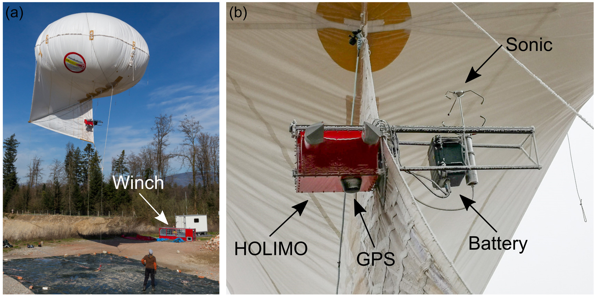
Figure 1Experimental setup of the HoloBalloon platform consisting of a tethered balloon system (a) and the instrument package (b). The winch is visible in the left picture. The instrument package includes the holographic cloud imager HOLIMO 3B, a 3-D sonic anemometer as well as a temperature and humidity sensor (not visible). The left picture has been taken by Pascal Halder (naturphotos.ch)
In this paper, we present a newly developed measurement platform for boundary layer clouds (HoloBalloon), consisting of a holographic cloud imager and a meteorological instrument package on a kytoon. Kytoons are a hybrid balloon–kite combination allowing stable flight at wind speeds up to 30 m s−1. The stability in high wind speeds makes kytoons a promising measurement platform for cloud research, especially in locations with strong wind conditions (e.g., mountain regions). Due to the low aspiration velocities of TBSs, the choice of the instrument is of particular importance, since fluctuations in wind speed and direction could influence the measurements. Most cloud probes use an inlet to ensure a steady sampling velocity in fluctuating wind speeds (Baumgardner et al., 2011). However, the use of inlets increases measurement uncertainty, due to size-dependent particle losses at the inlet and non-isokinetic sampling effects. One technique that overcomes this problem is digital in-line holography, which provides a well-defined sample volume independent of particle size and aspiration velocity, making holographic cloud imagers particularly well suited for measurements on TBSs. Digital in-line holography can simultaneously capture single particle information (position, size and shape) of an ensemble of cloud particles within a three-dimensional detection volume. Thus, it provides information of the phase-resolved particle size distribution (e.g., Beck et al., 2017), as well as the spatial distribution of an ensemble of cloud particles within a cloud volume on a millimeter scale (e.g., Beals et al., 2015). More detailed information about the working principle of a holographic imager will follow in Sect. 3.1. Digital holographic cloud imagers have been used in previous field campaigns on ground-based (e.g., Thompson, 1974; Kozikowska et al., 1984; Borrmann et al., 1993; Raupach et al., 2006; Henneberger et al., 2013; Schlenczek et al., 2017), airborne (e.g., Conway et al., 1982; Fugal and Shaw, 2009; Beals et al., 2015; Glienke et al., 2017; Desai et al., 2019) and cable car (Beck et al., 2017) platforms, but have not yet been deployed on TBSs.
The HoloBalloon platform merges the advantages of holography (well-defined sampling volume, spatial distribution of cloud particles) with the benefits of a TBS (high-resolution measurements) with the aim to observe the cloud structure on different scales. Information about the macroscopic cloud structure can be obtained from the vertical profiles up to 1 km above the ground, and information about the cloud microstructure can be extracted from the cloud particle spatial distribution within a single hologram. The HoloBalloon platform was tested in boundary layer clouds over the Swiss Plateau. Here we present observations of a case study during a stratus cloud event. The cloud structure is analyzed on different scales, starting with the large-scale cloud structure of tens of kilometers and moving down to the cloud microstructure on the meter scale. A particular emphasis is placed on cloud inhomogeneities. Previous observations found inhomogeneities in cloud properties on scales of a few tens of meters (e.g., Korolev and Mazin, 1993; Garcıa-Garcıa et al., 2002; Gerber et al., 2005) or even on the sub-meter scale (e.g., Baker, 1992; Brenguier, 1993; Beals et al., 2015; Beck et al., 2017; Desai et al., 2019), which were attributed to different physical processes such as turbulent mixing or entrainment. These microphysical signatures can have important implications for the cloud structure. For example, on a millimeter scale, they can be of importance for particle growth by collision–coalescence and thus for the efficiency of precipitation formation. Inhomogeneities at scales of hundreds of meters and kilometers can be important for radiative heating and cooling. In this paper, we investigate inhomogeneities in the microphysical properties of stratus clouds and aim to understand the formation mechanisms of such inhomogeneities. Throughout this study, inhomogeneities are defined by the variability in the cloud droplet number concentration and cloud droplet size.
The first part of the paper introduces the HoloBalloon measurement platform (Sect. 2). The working principle and the setup of the newly developed holographic cloud imager is described in Sect. 3. Observations of a case study in stratus clouds obtained with HoloBalloon are presented in Sect. 4. On the basis of these observations, the potential of the HoloBalloon platform in studying boundary layer clouds is discussed in Sect. 5.
The HoloBalloon platform is designed to obtain vertical, in situ profiles of the microphysical and meteorological cloud properties of boundary layer clouds up to 1 km above ground. Our TBS consists of a 175 m3 kytoon (Desert Star, Allsopp Helikite, UK), a 1200 m long Dyneema cable, and a gasoline winch to launch and recover the TBS (see Fig. 1). The balloon has a net lift of 85 kg at sea level. Kytoons are a hybrid combination of a helium balloon and a kite, exploiting both for lift. The helium balloon creates static lift, while the kite creates aerodynamic lift in wind. The kite utilizes a long keel to provide stability in high-wind conditions. The maximum operational wind speed of our TBS is 25 m s−1. So far, we operated the TBS in wind speeds of up to 15 m s−1. A further advantage of the kite is that it ensures that the instrument platform is oriented into the wind, allowing for the spatial distribution of cloud particles to be assessed.
The cable and winch are designed to withstand forces up to 4 t, which can occur during high-wind-speed conditions (> 15 m s−1). The 7 mm Dyneema cable has a length of 1200 m and a breaking strength of 8200 kg. At wind speeds larger than 5 m s−1, the TBS can have a flight angle of up to 45∘ due to the kytoon design, reducing the maximum flight height to 850 m. A system of three Platipus anchors is used to secure the balloon to the ground. The tethered balloon is launched and retrieved with a winch powered by a V8 Chevy engine (Skylaunch, UK). The winch has a line speed of 1 m s−1 forward and reverse, which allows a vertical profile of 500 m in 8 min.
The instrument package is installed at the keel of the HoloBalloon platform. The key component is the HOLographic Imager for Microscopic Objects (HOLIMO) (see Sect. 3) which can measure phase-resolved cloud properties. Additionally, the HoloBalloon platform is equipped with a meteorological instrument package (see Fig. 1) consisting of a 3-D sonic anemometer (Thies, 4.3830.20.340) and a heated temperature and humidity sensor (HygroMet4, Rotronic) in an actively ventilated radiation shield (RS24T, Rotronic). The platform is powered by a 1000 W h battery, which allows for continuous operation of the instrument package for up to 5 h. Data are temporally stored on a 4 TB solid-state drive, and a mobile router enables remote access of the platform via a mobile data network connection (similar to Beck et al., 2017). The HoloBalloon instrument platform has a total weight of about 22 kg, consisting of the HOLIMO 3B instrument (13 kg), the meteorological instrumentation (5 kg) and the battery pack (4 kg).
To obtain reliable measurements of wind speed and direction, the motion of the balloon needs to be removed (e.g., Canut et al., 2016). Here we used a GPS antenna (TW3740, Tallysman) and an inertial navigation system (Ellipse2-N, SBG Systems) to measure the position, velocity and orientation of the instrument package. The GPS antenna and the inertial navigation system are fixed on the HOLIMO 3B instrument and are thus an integral part of the instrument package. We followed the procedure described in Elston et al. (2015) to convert the wind measurements from the inertial frame to the sonic anemometer frame and thus to correct for the motion of the balloon. The corrected wind measurements are presented and compared to other wind observations in Sect. 4.2.
The main component of the HoloBalloon instrument package is the holographic cloud imager HOLIMO 3B, which can image cloud particles between 6 µm and 2 mm within a three-dimensional detection volume. Despite its open-path configuration, HOLIMO 3B has a velocity-independent well-defined sample volume. This property makes HOLIMO 3B particularly well suited for application on a TBS due to fluctuating aspiration speeds towards a TBS.
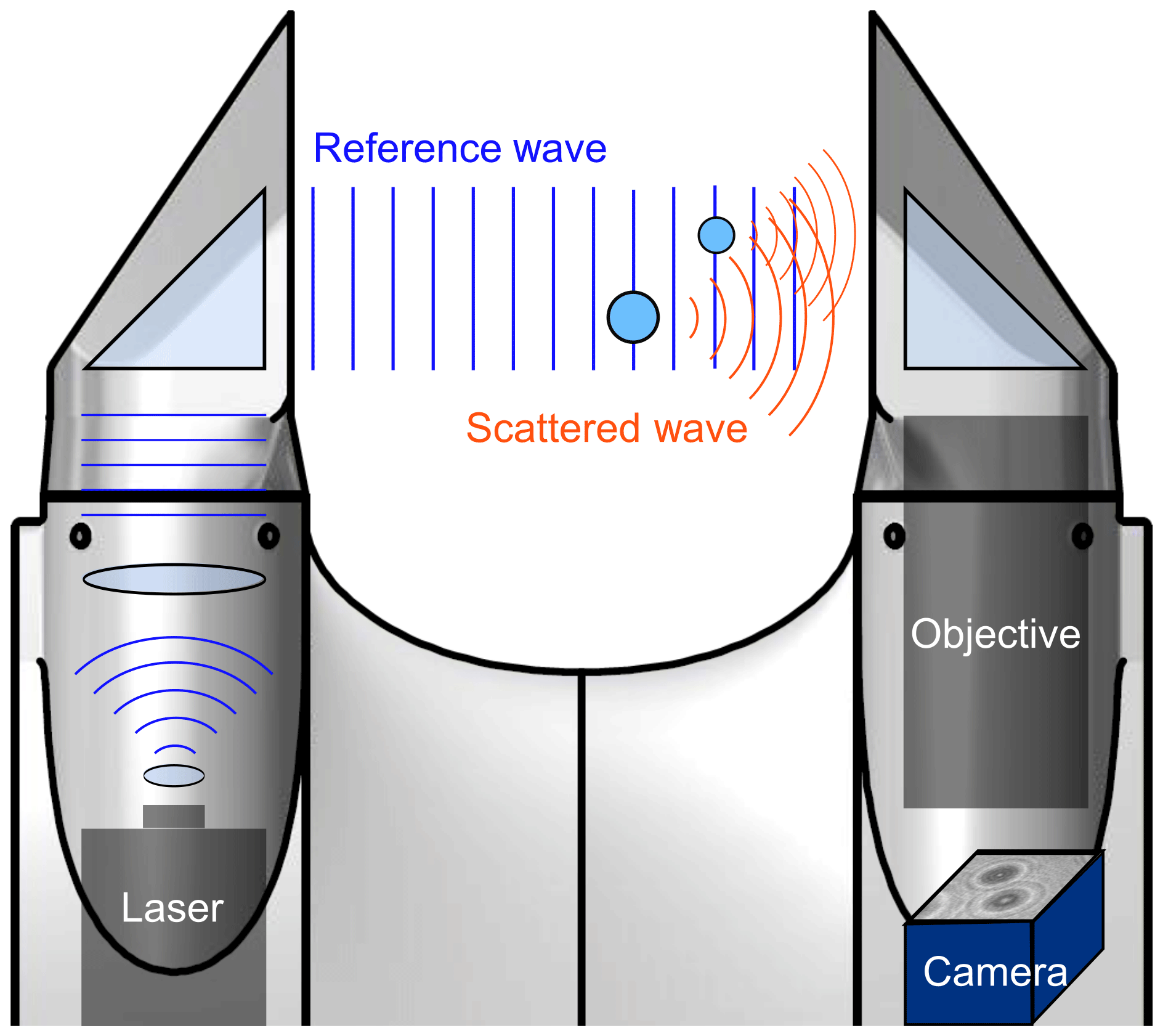
Figure 2Schematic of the working principle of digital in-line holography. A collimated laser beam is scattered by two particles. The scattered waves interfere with the reference wave and form an interference pattern (i.e., a hologram) which is recorded by a digital camera.
3.1 Working principle of digital in-line holography
HOLIMO 3B works on the principle of digital in-line holography (Fig. 2), which consists of a two-step process requiring a coherent light source and a digital camera. In the first step, the interference pattern of a reference wave (laser) and scattered waves (the light scattered by cloud particles in the sample volume) is recorded as a hologram. The second step involves a reconstruction process, in which the 2-D shadowgraphs and 3-D in-focus position of the particles are extracted from the interference pattern, using the HoloSuite software package (Fugal et al., 2009; Schlenczek, 2018). The resulting 2-D shadowgraphs can be classified as cloud droplets, ice crystals and artefacts based on a set of parameters using supervised machine learning (e.g., Fugal et al., 2009; Beck et al., 2017; Touloupas et al., 2019). In the present study, a set of around 7000 particles was classified manually, which served as a training data set on support vector machines. From the classification, the phase-resolved particle size distribution is computed. The particle diameter is calculated based on the number of pixels (see also Sect. 3.3) and the number concentration can be computed from the particle counts within the well-defined sample volume. Only particles that exceed a size of 2×2 pixels (6 µm) are considered. Moreover, because holography provides a snapshot of an ensemble of cloud particles, the spatial distribution of the cloud particles can be recovered from the interference pattern. Unlike light scattering instrumentation, no assumptions about the particle shape, orientation or refractive index are required, because an image of the cloud particles is recorded. The major disadvantage of holography is the high computational power associated with the reconstruction process and the data analysis. The working principle of digital in-line holography and HOLIMO has been described in more detail in Fugal et al. (2009), Henneberger et al. (2013) and Beck et al. (2017).

Figure 3Optical resolution measurements of the HOLIMO 3B instrument as a function of the reconstruction distance. The blue dots represent the resolutions measured with a US Air Force resolution target 1951 USAF (Dres,obs). The three lines indicate theoretical resolution limits due to the pixel size (Dres,pixel, red solid line), the optical limitation of the lens system (Dres,lens, gray dashed line) and the optical setup of the instrument (Dres,rec, black solid line). The strongest resolution limit constraint determines the optical resolution of the instrument at a specific reconstruction distance. More information about the theoretical resolution constraints for holographic systems can be found in Henneberger et al. (2013) and Beck et al. (2017).
3.2 Instrument description
A series of holographic instruments have been developed in the Atmospheric Physics group at ETH Zurich in the last decade (Amsler et al., 2009; Henneberger et al., 2013; Beck et al., 2017). HOLIMO 3B consists of two main units: the control unit, which comprises the temperature control system and the control and data-acquisition computer, and the optical imaging unit, which is integrated in the two instrument towers. Like the previous version (HOLIMO 3G; Beck et al., 2017), HOLIMO 3B has an open-path configuration. In contrast to the previous versions, HOLIMO 3B uses a 355 nm laser and an improved optical system to enlarge the detection volume and improve the optical resolution of the instrument.
A schematic of the optical system of HOLIMO 3B is shown in Fig. 2. The laser (FTSS355-Q4_1k, CryLaS, Germany) emits pulses with a wavelength of 355 nm, with a pulse width of 1.4 ns and a pulse energy of 42 µJ. The beam is attenuated by a neutral density filter and focused through a 10 µm diamond pinhole (Lenox Laser HP-3/8-DISC-DIM-10), which acts as a point light source. The diverging laser beam is expanded by a biconcave lens and collimated to a beam diameter of around 40 mm. After passing through a turning prism and a sapphire window, the collimated laser beam traverses the sample volume, before entering the imaging lens system in the opposite tower of the instrument. The bi-telecentric lens system (Correctal S5LPJ2755, TDL65/1.5 UV, Sill Optics, Germany) has a magnification of 1.5 and a numerical aperture of 0.13. The holograms are recorded with a 25 MP camera (hr25000MCX, SVS-Vistek, Germany) with 5120×5120 pixels, a pixel pitch of 4.5 µm and a maximum frame rate of 80 fps (frames per second). The quadratic cross-sectional area of the camera allows for more uniform illumination of the edges than a rectangular camera image, which was used in the previous versions.
The optical resolution of the system was tested using a US Air Force resolution target (1951 USAF), which is placed at different positions inside the detection volume, following the procedure described in Spuler and Fugal (2011) and Beck et al. (2017). The optical system described achieves a resolution (Dres,obs) of 6 µm within the first 110 mm of the reconstruction distance (see Fig. 3). This is consistent with the theoretical resolution limit of the pixel size (Dres,pixel). For reconstruction distances larger than 110 mm, the resolution limit decreases and is determined by the resolution limit from the diffraction aspects of in-line holography (Dres,rec). In general, the measured optical resolutions are in good agreement with the theoretical resolution constraints. Particles within the first 10 mm and close to the image border (<0.2 mm from image edges) are not included in the analysis due to flow distortion effects from the towers and edge effects. With an effective cross-sectional area of 15 mm×15 mm and an effective depth of 100 mm, this results in a sample volume of 22.5 cm3 and a maximum sample volume rate of 1800 cm3 s−1 (with 80 fps).
3.3 Size calibration of HOLIMO 3B
Accurate sizing of cloud particles is important to obtain reliable measurements of cloud properties such as water content and size distributions. For holographic instruments, the sizing algorithm should be precise and accurate over a large particle size range (6 µm – 1 cm) and applicable for the entire detection volume. The sizing of the particles strongly depends on an amplitude threshold value that separates particle pixels from background pixels. From the number of particle pixels, the area-equivalent diameter is derived. In the standard HoloSuite version, a uniform amplitude threshold is used for particle detection and particle sizing. However, a uniform amplitude threshold leads to unsatisfying results for particle sizing due to a decreasing signal-to-noise ratio with increasing reconstruction distance z in the large detection volume of HOLIMO 3B. This has the effect that the amplitude image of the particles becomes less distinct with larger z distances, and thus the observed particle size decreases with increasing z distance. To overcome this issue and to ensure a uniform sizing of the particles over the entire detection volume, Beck (2017) introduced a new method by normalizing the in-focus particle image. In the normalization step, the darkest particle pixel is set to 0 (black), the mean of the background pixels is set to 1 (white) and the rest of the pixels are scaled relatively. This results in a more uniform signal-to-noise ratio and allows the application of a uniform amplitude threshold. The amplitude threshold can be used as a tuning parameter to calibrate the sizing algorithm of the HoloSuite software for the HOLIMO 3B instrument.
Table 1Results of the size calibration experiments of HOLIMO 3B and an APS. The mean diameter and the standard deviation are derived from a Gaussian fit to the normalized size distribution.
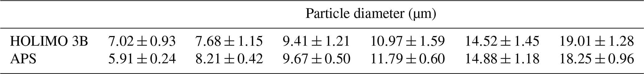

Figure 4Size distributions from calibration experiments of the HOLIMO 3B instrument. The symbols show the normalized particle concentration measured by HOLIMO 3B (filled) and the APS (unfilled) instrument. The lines indicate the Gaussian distributions fitted to the HOLIMO 3B data (solid) and APS data (dashed). The numbers represent the mean diameter of the APS size distribution.
The sizing algorithm was calibrated using a vibrating orifice aerosol generator (VOAG model 3450, TSI, Minnesota, USA) for particle generation and an aerodynamic particle sizer (APS model 3321, TSI, Minnesota, USA) for particle sizing. Particles with diameters between 5 and 18 µm were generated by the VOAG using a liquid oil–water solution. The generated particles were introduced into a 120 mm×1000 mm cylindrical tube and measured by the HOLIMO 3B instrument and an APS that were installed at the end of the tube. The APS covers the size range between 1 and 20 µm and is used as a reference measurement. The amplitude threshold was used as a tuning parameter to fit the HOLIMO 3B measurements to the APS measurements. An amplitude threshold of 0.47 was found to fit the APS data best (smallest sum of squared errors). The size distributions of the calibration experiments are shown in Fig. 4 and are summarized in Table 1.
The size distributions of the HOLIMO 3B and APS instruments were normalized to their maxima, and a Gaussian distribution was fitted to the data. The results of the HOLIMO 3B instrument agree with the mean diameter of the APS within instrumental uncertainty. In general, a trend towards an underestimation of the particle diameter compared to the APS is observed, except for the calibration measurements at the measurement limits of HOLIMO 3B (6 µm) and the APS (18 µm). The overestimation of the particle diameter by HOLIMO 3B for 6 µm particles may be due to the optical resolution limit of the HOLIMO 3B instrument. While HOLIMO 3B can only detect particles larger than 6 µm, the APS can detect particles down to a diameter of 1 µm. On the other hand, the overestimation of the particle diameter at 18 µm could be caused by a bias of the APS instrument, which has an upper detection limit of 20 µm. Thus, particles in the second peak at 23 µm are not detected by the APS (see Fig. 4). To conclude, no correction to the sizing algorithm was made, because all size measurements agree within the square root of the pixel size ().
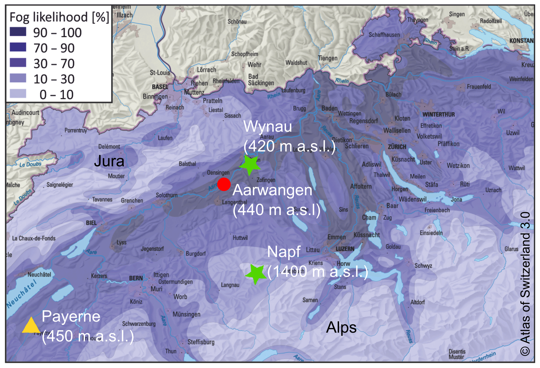
Figure 5Map of the fog frequency during winter (adapted from the “Atlas of Switzerland 3.0”, 2010, https://www.atlasderschweiz.ch/, last access: 24 January 2020) and of the measurement locations. The climatology of fog is based on satellite images. The field locations include the measurement site in Aarwangen from which HoloBalloon was launched (red circle), ground-based weather stations from MeteoSwiss providing measurements of meteorological parameters (green stars) and the field site in Payerne from which radiosondes are launched twice a day (yellow triangle).
As a case study, we present observations of a supercooled low stratus cloud event (also referred to as high fog) during a Bise situation over the Swiss Plateau, obtained on 24 February 2018 between 08:00 and 10:00 UTC. Bise is a typical weather situation in Switzerland during winter (Wanner and Furger, 1990). The case study focuses on nine vertical profiles of microphysical and meteorological cloud properties measured by the HoloBalloon platform. The analysis starts with an overview of the synoptic weather situation and the large-scale cloud structure and moves towards smaller scales, providing information about the cloud microstructure.
The Swiss Plateau, which lies between the Jura mountains and the Swiss Alps, is often covered by fog or low stratus clouds during fall and winter due to its geographic location. A satellite-based climatology of fog and low stratus cloud coverage over the Swiss Plateau during high-pressure situations in winter is shown in Fig. 5. In regions along rivers and lakes, a fog frequency of up to 90 % is observed. Most commonly, fog forms by radiative cooling during clear nights. Additionally, cold air flows from the Alpine valleys and the Jura towards the Swiss Plateau, where the cold air can accumulate. This cooling of the air can cause condensation and the formation of ground fog. However, the case study presented here was connected to a Bise situation; a cold, dry east-northeast wind. During Bise, cold air is advected and pushed under warm air, leading to the formation of a strong temperature inversion. The cold air in the lower layer cannot easily escape the Swiss Plateau because it is bound by the Jura mountains and the Swiss Alps. If the air is sufficiently moist, condensation sets in and fog or low stratus clouds can develop. The top of the cloud layer is defined by the height of the temperature inversion. The solar radiation reaching the boundary layer is often too weak to dissipate the fog layer in fall and winter. Thus, ground fog or stratus clouds can persist for several days, until a change in the synoptic weather pattern occurs.
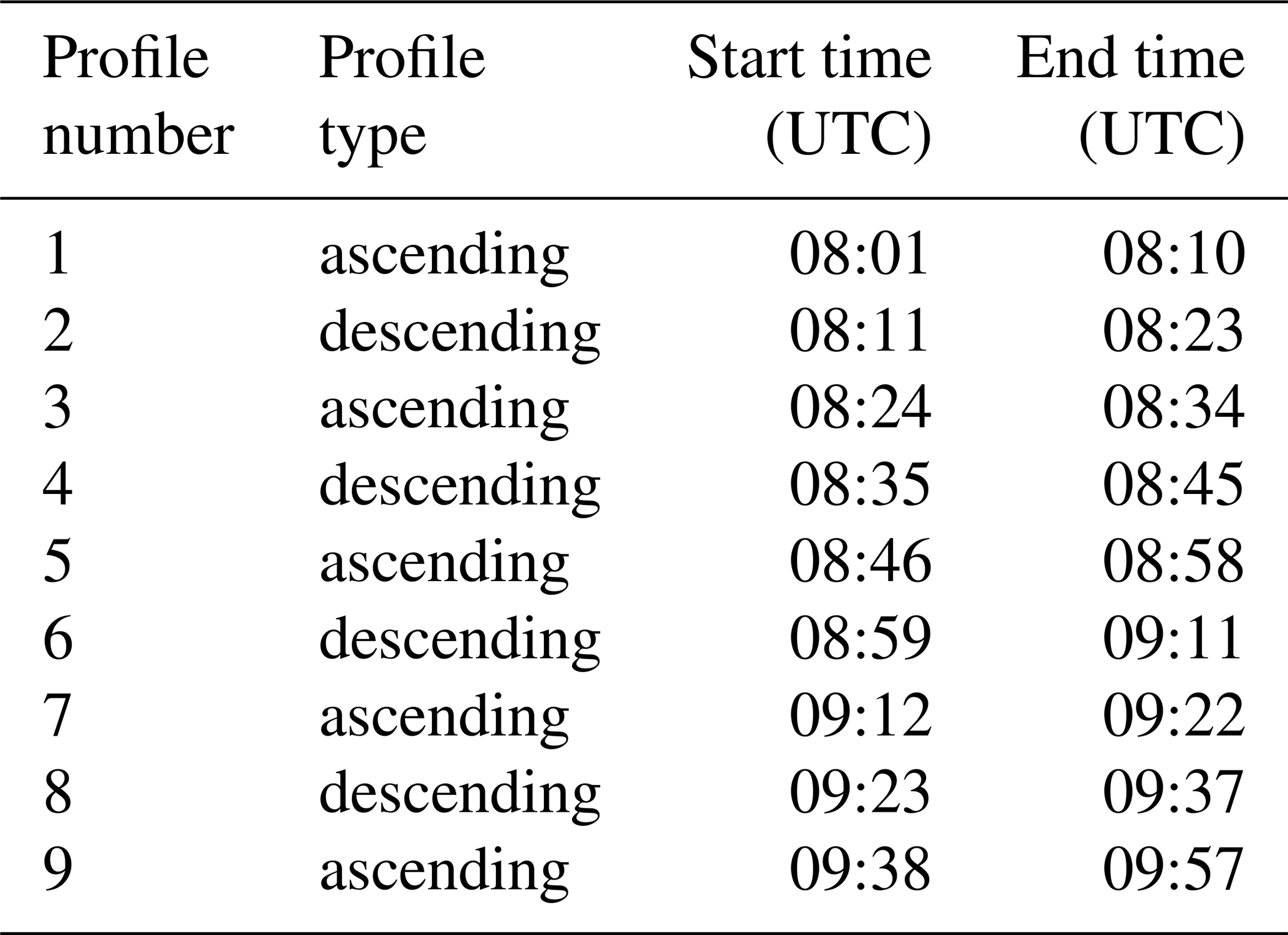
Table 2Summary of the start and end time of the nine vertical profiles observed with the HoloBalloon platform.
4.1 Measurement location and data analysis
The measurements with the HoloBalloon platform were performed in Aarwangen (47∘14′ N, 7∘45′ E) in the Swiss Plateau 40 km northeast of Bern (Fig. 5). The field site is located at a gravel station next to the Aare river at an altitude of 440 m a.s.l. and is surrounded by grassland and forests. The balloon measurements were performed in a temporarily closed air space of 2 km in diameter, which was activated on measurement days. The maximum flight height allowed was 700 m above ground because of air traffic regulations. The experimental setup of the HoloBalloon platform is shown in Fig. 1.
The measurements taken on the HoloBalloon platform were complemented and validated by observations of surrounding MeteoSwiss weather stations and radiosondes (see Fig. 5). The weather stations are located within a radius of 30 km from Aarwangen and cover altitudes between 420 and 1400 m a.s.l. Radiosondes are launched twice a day (00:00 and 12:00 UTC) from Payerne, which is located 80 km southwest of Aarwangen. We used the radiosondes to determine the inversion and cloud top height, because we were not able to measure the whole cloud layer due to the air traffic restrictions on flight height.
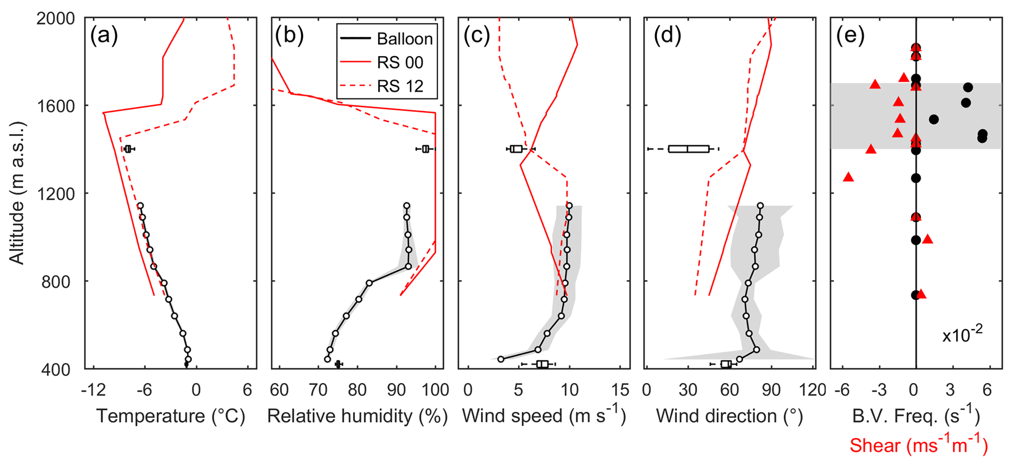
Figure 6Vertical profiles of the meteorological parameters (a–d). The HoloBalloon measurements are averaged over nine profiles and an altitude interval of 75 m. The black dots indicate the mean and the shaded area the standard deviation of the data. The vertical profiles of two radiosonde ascents (00:00 UTC (solid) and 12:00 UTC (dashed)) are shown by the red lines. The box plots represent the data from MeteoSwiss weather stations (Wynau (420 m a.s.l.), Napf (1400 m a.s.l.)). In each box, the central line indicates the median, and the left and right edges of the box mark the 25th and 75th percentiles, respectively. The whiskers extend to the minimum and maximum of the data not considered as outliers. Panel (e) shows the vertical profile of the Brunt–Väisälä frequency () and the wind shear () calculated from the radiosonde ascent at 12:00 UTC. The shaded area in (e) indicates regions with a positive Brunt–Väisälä frequency.
A total of nine vertical profiles measured with the HoloBalloon platform were analyzed in this case study, with an average of 800 holograms (∼5 L sampled volume) or 600 000 cloud particles per profile. The battery of the instrument package was empty after profile 9; thus no observations were available afterwards. Each profile had a duration of 10–15 min. With a mean horizontal wind speed of 10 m s−1, this results in a horizontal resolution of around 6–9 km. The start and end times of the individual profiles are summarized in Table 2. At least 10 holograms were grouped together to obtain better counting statistics. This results in a vertical resolution of 5 m. Only data points with a liquid water content (LWC) larger than 0.01 gm−3 (definition for cloud base) are considered in the analysis. Cloud particles smaller than 25 µm were classified into the three categories of cloud droplets, ice crystals and artifacts using support vector machines (see Sect. 3.1), whereas particles larger than 25 µm were classified manually (visual classification). Only particles within a reconstruction distance between 20 and 50 mm were included in the analysis. A smaller detection volume than described in Sect. 3.2 was chosen due to the mean droplet size being close to the instrumental resolution limit and noise in the holograms.
4.2 Meteorological situation
Figure 6 shows vertical profiles of the meteorological parameters during the measurement period. The meteorological conditions during the 2 h measurement period were relatively stable. The temperature profile was characterized by a strong temperature inversion, which was located at around 1450 m a.s.l. The temperature varied between −1 ∘C at the surface and −8.9 ∘C at the inversion base. The height of the temperature inversion defines the top of the cloud layer. The relative humidity increased from the ground up to 850 m a.s.l., where it remained constant up to the inversion. We assumed that this constant relative humidity interval indicates conditions of water saturation and thus marks the extent of the cloud layer. No relative humidity values above 95 % were observed by the HoloBalloon platform. This can be explained by the challenges of measuring relative humidity at in-cloud conditions (e.g., Korolev and Mazin, 2003; Korolev and Isaac, 2006). Wind speeds between 6.7 and 8.6 m s−1 were observed in Wynau with wind gusts up to 10.6 m s−1. The wind speed in Aarwangen increased in the first 200 m above the ground from 7 to 10 m s−1. As it can be seen from the radiosondes, the wind speed was relatively constant up to the inversion layer. The prevailing wind direction was northeast with a slight turn towards east with increasing altitude. At the inversion, a change in the horizontal wind speed and direction with height (vertical wind shear) occurs. In this region, a positive Brunt–Väisälä frequency N is observed (Fig. 6e). These conditions are favorable for the development of boundary layer waves and Kelvin–Helmholtz instability (see Sect. 4.4).
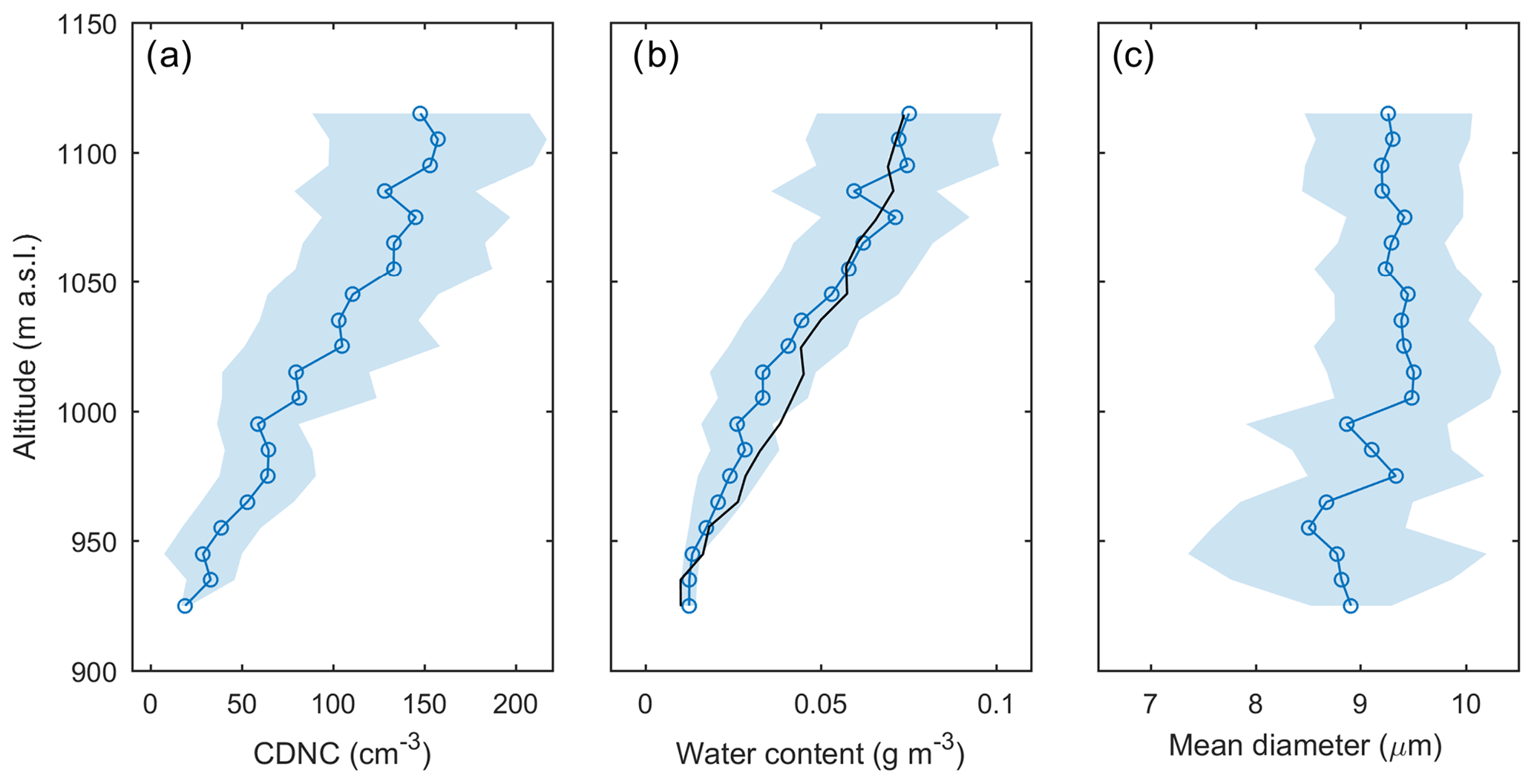
Figure 7Mean vertical profiles of the cloud droplet number concentration (a), liquid water content (b) and mean cloud droplet diameter (c) averaged over the nine profiles measured with the HoloBalloon platform. The data are averaged over an altitude interval of 10 m. The shaded area represents the standard deviation. The black line in (b) shows the adiabatic LWC profile wl_ad, which is obtained as follows: (i) calculate the saturation vapor pressure es at the cloud base, (ii) use the pressure at the cloud base to determine the saturation mixing ratio , (iii) calculate at the cloud base assuming wl = 0.01 g kg−1 and assuming constant wt with height (adiabatic), and (iv) calculate ws at all height levels, determine wl and multiply wl by local dry air density to obtain wl_ad.
4.3 Microphysical cloud structure
Figure 7 shows the mean vertical profiles of the microphysical cloud properties averaged over nine profiles. The mean cloud droplet number concentration (CDNC) increases from 10 cm−3 at the cloud base (920 m) to 150 cm−3 at 1100 m (Fig. 7a). The mean liquid water content (LWC) ranges between 0.01 and 0.08 g m−3 and on average approaches an adiabatic profile (Fig. 7b). The mean cloud droplet diameter increases from 9 to 9.5 µm between the cloud base and 1000 m and stays constant above (Fig. 7c). The observed CDNC of 150 cm−3, LWC of 0.08 g m−3 and mean cloud droplet diameter of 9.5 µm are in the observed range for fog and continental stratus clouds (Lohmann et al., 2016), but rather at the lower end of the range. Despite the supercooled conditions, only a few ice crystals were observed (<1 L−1).
The increase in CDNC with increasing height is in contrast to the theory of an adiabatic cloud profile and might be explained by different factors. An adiabatic cloud model assumes that cloud droplets activate at the cloud base and grow in size with increasing altitude. Thus, CDNC is expected to remain constant with height after the maximum supersaturation is reached. There are several possibilities why this theoretical concept is not applicable for the case study presented here. Firstly, HOLIMO 3B does not detect cloud droplets smaller than 6 µm. This can lead to an underestimation in CDNC, especially at cloud base where the droplets are the smallest. Secondly, an adiabatic cloud model assumes a constant updraft, but fluctuations in the updraft speed or turbulence could generate supersaturated conditions and activate cloud droplets at higher altitudes than cloud base. Thirdly, the increase in CDNC with height could be driven by radiative cooling at the cloud top by producing either supersaturation or instabilities and thus turbulence within the cloud layer. On the other hand, a database of stratus clouds (Miles et al., 2000) showed that the CDNC in continental clouds was more variable with height than in marine clouds where CDNC was determined near cloud base. Therefore, it is unclear whether the observed increase in CDNC is a measurement artifact or a real feature of the observed cloud. Regardless, we recommend that future balloon-borne measurements of clouds include instruments capable of measuring even the smallest cloud particles.
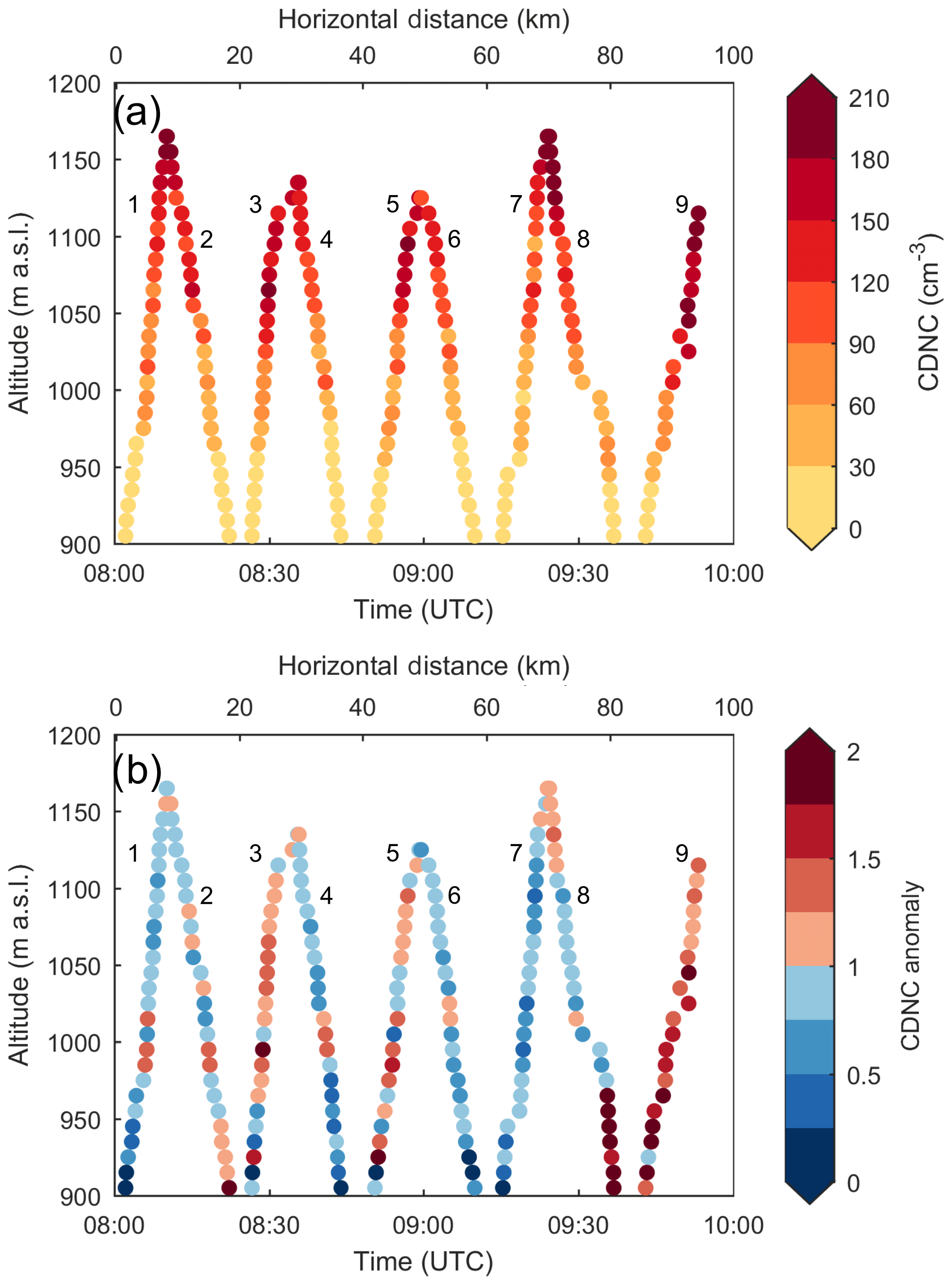
Figure 8Height-temporal evolution of the CDNC (a) and the CDNC anomaly (CDNC, b) (see text for explanation of anomaly). The data points are averaged over an altitude interval of 10 m. The upper x axis shows the horizontal distance s of the cloud, assuming a mean wind speed v of 10 m s−1 over time t (). The numbers represent the profile number according to Table 2.

Figure 9Vertical profile of CDNC (in red) and CDNC anomaly (in black, CDNC) (a) and number size distribution (b) of profile 7. To the left of the dashed vertical line in (a), CDNC is less than 0.5. The data are averaged over a 10 m interval. The black rectangle in (b) shows the region of decreased CDNC (discussed in text).
4.4 Inhomogeneities in the microphysical cloud properties of stratus clouds
Upon further analysis, we investigate cloud inhomogeneities in stratus clouds on different scales and discuss potential physical processes, which could influence these cloud signatures. In the present study, cloud inhomogeneities are defined by the variability in the CDNC. Therefore, we introduce the term CDNC anomaly (CDNC), which describes the variability of the CDNC over a given height interval h. The CDNC is calculated by dividing the CDNC observed in the height interval h (CDNCh) by the mean CDNC in that height interval averaged over the nine profiles () (i.e., CDNC = CDNC). As Korolev and Mazin (1993), we define areas with CDNC as regions of decreased CDNC and areas with CDNC as regions of increased CDNC.
The height-temporal evolution of the CDNC and CDNC is shown in Fig. 8. CDNC reveals areas of increased and decreased CDNC. For example, profile 7 shows regions of decreased CDNC, whereas profile 9 shows regions of increased CDNC compared to the mean profile. The CDNC at 1100 m in profile 9 (200 cm−3) is more than a factor of 3 higher than in profile 7 (60 cm−3). From a single profile perspective, all profiles show alternating regions of higher and lower CDNC. It is likely that the observed variations in CDNC exceed statistical variations and are the result of different physical processes.
The variability in CDNC on a scale of several kilometers might be explained by the presence of boundary layer waves. Boundary layer waves can cause entrainment of dry air into the cloud (Mellado, 2017) and could affect the cloud structure (e.g., Bergot, 2013). As discussed for example by Wanner and Furger (1990), strengthening or weakening of the Bise due to dynamic effects could induce oscillations within the cold air and lead to the formation of boundary layer waves at the cloud top. The presence of wind shear and a positive Brunt–Väisälä frequency (N=0.04 s−1) at the inversion (see Fig. 6e) represent favorable conditions for the formation of Kelvin–Helmholtz instability and boundary layer waves. However, in order to further test this hypothesis, microphysical observations up to cloud top and an extended set of auxiliary measurements (e.g., three-dimensional wind field, turbulence) over a time period of several hours would be necessary.
Inhomogeneities in CDNC on a meter scale can be the result of different processes, depending on their location within the cloud. We will discuss these cloud inhomogeneities based on profile 7, because it has CDNC below 1 almost everywhere (see Fig. 8b). Profile 7 shows a gradual increase in cloud droplet size and number concentration with height until a sudden decrease in particle concentration and cloud droplet size occurs between 1070 and 1130 m (Fig. 9b). In this region, CDNC is less than half of the average CDNC (CDNC, Fig. 9a). In addition, the cloud droplet spectrum shows an increase in small droplets and an absence of cloud droplets larger than 14 µm. Korolev and Mazin (1993) propose several mechanisms for the formation of cloud inhomogeneities on a meter scale such as (i) entrainment, (ii) variability of the condensation level and (iii) evaporation in descending motions. Considering the location of our region of decreased CDNC (300–400 m from cloud top, 200 m from cloud base), we assume that this CDNC below 1 is most likely formed by evaporation in descending motions. The temperature inside a descending air parcel increases due to adiabatic compression and heating, and in response cloud droplets evaporate, leading to regions of decreased CDNC. However, more sophisticated analyses of turbulence and microphysical observations up to cloud top are required to further investigate these cloud inhomogeneities and the corresponding physical processes, which is beyond the scope of this study.
5.1 Validation of the HoloBalloon platform and further improvements
The HoloBalloon platform was successfully deployed in various meteorological conditions. In situ profiles up to 700 m altitude above the ground were obtained, limited by air traffic restrictions in the maximum altitude. Unfortunately, because of this limitation in the maximum altitude, we were not able to penetrate the whole cloud layer and perform measurements at the cloud top. The platform was deployed at temperatures down to −8 ∘C. Despite the supercooled conditions, we observed only a few ice crystals (<1 L−1). Even though parts of the balloon and of the cable were covered in ice, this did not affect our measurements and the flight performance. However, based on our experience, we recommend covering the balloon with a tarp at night to prevent accumulation of snow and water on the balloon. We flew the TBS in wind speeds up to 15 m s−1. The TBS was stable in these high-wind conditions, but the ground handling became challenging at wind speeds above 10 m s−1, especially in the presence of wind gusts.
For setting up and operating the HoloBalloon platform, several aspects need to be considered. Firstly, a closed air space was required to perform cloud measurements with a TBS. The process of obtaining a closed air space was closely coordinated with the aviation safety authority. In areas with dense air traffic, such as the Swiss Plateau, it can be difficult to find a suitable location. Secondly, a large, reasonably flat surface area () is required to prepare and launch the TBS. No major obstacles (e.g., trees, power lines) should be within a radius of around 60 m of the launching site and it should be possible to insert an anchor into the ground. The system set up takes approximately 3 d and requires two to three trained persons for operation. A third person can especially be helpful during difficult wind conditions.
HoloBalloon was able to measure temperature, relative humidity and wind profiles in boundary layer clouds. In general, the measurements agreed well with the observations from the MeteoSwiss weather stations and the radiosondes (see Fig. 6). The temperature sensor showed a delayed response to changes in the ambient temperature (not shown), similarly to what was observed by Beck et al. (2017) on the cable car platform HoloGondel. To overcome this issue, the temperature was calculated from the virtual temperature of the 3-D sonic anemometer, assuming water saturation in the cloud. It is well known that it is difficult to measure relative humidity in clouds (e.g., Korolev and Mazin, 2003; Korolev and Isaac, 2006). The relative humidity measured by the HoloBalloon platform in clouds ranged between 93 % and 98 %. We assumed in-cloud conditions when the relative humidity remained constant with height. Wind speed and direction measurements of the 3-D sonic anemometer were corrected for the motion of the balloon. As described in Sect. 2, this was done using the output from an inertial navigation system and a GPS antenna following the procedure described in Elston et al. (2015). The corrected horizontal wind speed and wind direction measurements agreed well with the radiosonde observations. Vertical wind speed and turbulence measurements were not considered in this study, because we cannot exclude an influence from the balloon on the turbulence measurements, as the instrument package was installed on the keel below the balloon (Fig. 1). For future field campaigns, we will install the instrument package 20–30 m below the balloon in order to minimize potential influences from the balloon and to also analyze turbulence data of the 3-D sonic anemometer. The feasibility of a hanging mount was already successfully tested in the field in the fall of 2019.
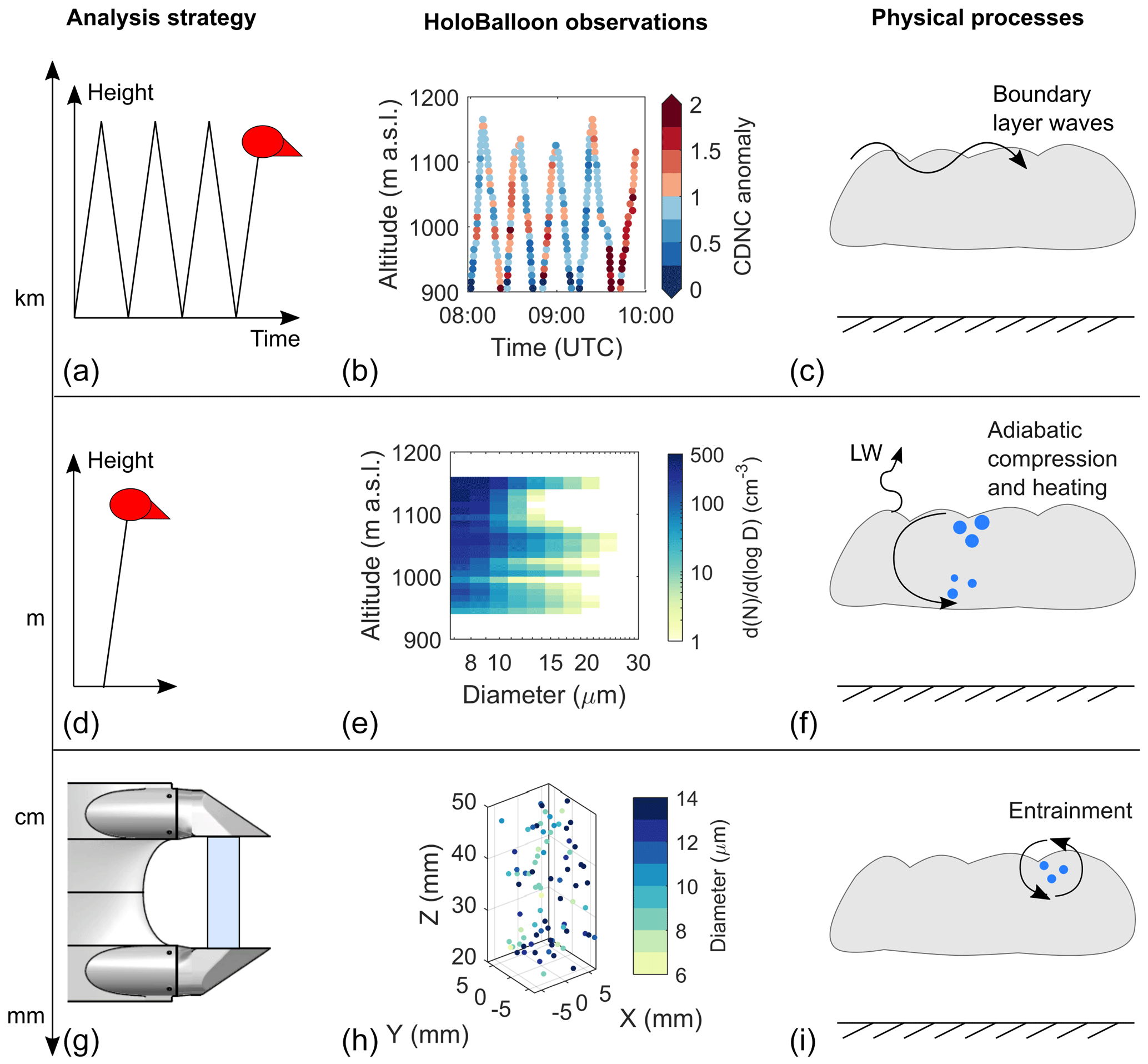
Figure 10Conceptual picture describing the potential of the HoloBalloon platform in studying boundary layer clouds. It shows the scale-dependent analysis strategy (a, d, g), exemplary HoloBalloon observations of the presented case study (b, e, h) and possible physical processes that can be studied with the HoloBalloon platform (c, f, i). The scale-dependent analysis strategies include the analysis of a series of vertical profiles (a, b, c), a single vertical profile (d, e, f) and a single hologram (g, h, i).
The vertical profiles of the microphysical measurement showed no systematic difference between ascending and descending profiles (see Fig. 8b), suggesting that the balloon was not significantly influencing the microphysical measurements themselves. With a mean horizontal wind speed of 10 m s−1 and a cable speed of 1 m s−1, the horizontal wind speed is a factor of 10 larger than the cable speed. This, in combination with a flight angle of up to 45∘ (due to the kytoon design), minimizes shading effects and further supports the assumption that a “pristine” cloud volume is measured.
Generally, the measured size distributions during the present case study showed the maximum number concentration close to the resolution limit of HOLIMO 3B. This demonstrates the limits of the instrument in measuring small cloud particles (<6 µm). This bias can lead to an underestimation of CDNC, especially close to cloud base or in fog or clouds with a small mean cloud droplet diameter. For future field campaigns, we will equip the HoloBalloon platform with an optical particle counter in order to cover the entire cloud droplet size distribution.
5.2 Using the HoloBalloon platform to study boundary layer clouds
The potential of the HoloBalloon platform in studying boundary layer clouds is summarized in a conceptual picture (Fig. 10), which is described with the help of the presented case study. Based on the research questions, different analysis strategies can be applied. Firstly, by analyzing a series of vertical profiles, the HoloBalloon platform can investigate the temporal and spatial evolution of cloud properties on a kilometer scale (Fig. 10a, b, c). A vertical profile of 500 m can be accomplished within 8 min. Thus, a vertical profile can be obtained faster than with an aircraft. Secondly, individual profiles obtained with the HoloBalloon platform can provide information about the vertical cloud structure (Fig. 10d, e, f). With a sample rate of up to 80 fps and an aspiration speed on the order of 10 m s−1, the HoloBalloon platform can provide high-resolution measurements on the meter scale. We found that stratus clouds can exhibit complex dynamic structures with microphysical signatures on different scales (Sect. 4.4). For example, we observed a large variability in the CDNC and cloud droplet size within the stratus cloud. More sophisticated analyses of numerous cloud cases are required to further investigate cloud inhomogeneities and their physical implications. However, no generalization was possible in this study.
Furthermore, the analysis of individual holograms, or more specifically the analysis of the spatial distribution of an ensemble of cloud particles in the sample volume (Fig. 10g, h, i), allows the study of small-scale processes and particle–particle interactions. For example, a spatial distribution analysis can provide insights into the physical nature of the interface between cloudy and ambient air and thus can be used to study entrainment and turbulent mixing at the cloud top. However, a quantitative analysis of the spatial distribution (e.g., Larsen and Shaw, 2018; Larsen et al., 2018) is required to assess these small-scale processes, which is beyond the scope of this study. Future work will focus on the spatial distribution of cloud particles.
The HoloBalloon platform can be used to study processes over a wide range of scales from the kilometer down to the millimeter scale. However, the present case study also revealed some limitations of the HoloBalloon platform. For example, the vertical profiles are limited by the cable length (1200 m) or air traffic regulations regarding the maximum flight height (700 m) and it can only observe the cloud properties along the measurement path. In order to obtain a more comprehensive understanding of boundary layer clouds, a multidimensional set of instruments would be necessary. For example, the HoloBalloon measurements could be complemented by remote sensing instruments (e.g., cloud radar), which can provide continuous information of the large-scale cloud structure. Moreover, a wind profiler could be used to characterize the three-dimensional wind field and to identify dynamical patterns such as boundary layer waves. Such a multi-scale approach could help to improve the microphysical and dynamical understanding of boundary layer clouds in future field campaigns.
In this study, we have introduced the newly developed measurement platform HoloBalloon and have shown its ability and potential in studying boundary layer clouds. Here, we presented in situ observations of a supercooled low stratus cloud during a Bise event over the Swiss Plateau in February 2018. Our main findings are summarized as follows.
-
HoloBalloon merges the advantages of holography with the benefits of a TBS. Unlike other single-particle measurement techniques, holographic cloud imagers have a well-defined sample volume independent of particle size and air speed despite fluctuating aspiration speeds on a TBS. The low aspiration speed on the TBS in combination with the high acquisition rate of HOLIMO 3B allows for measurements with high spatial resolution.
-
The HoloBalloon platform was successfully deployed at temperatures down to −8 ∘C and wind speeds up to 15 m s−1. While conventional blimp-like TBSs are limited to wind speeds below 10 m s−1, kytoons are designed for wind speeds up to 25 m s−1, making them an interesting measurement platform for atmospheric research.
-
HoloBalloon was able to reliably measure in situ vertical profiles of the microphysical cloud properties and meteorological parameters up to 700 m above ground. The meteorological measurements agreed well with observations from radiosondes and weather stations, and the observed cloud properties were within the expected range for fog and stratus clouds. Cloud particles between 6 and 24 µm and CDNC up to 200 cm−3 were observed with HOLIMO 3B.
-
HoloBalloon was able to capture cloud inhomogeneities on different scales. For example, we observed a large variability in the CDNC and mean cloud droplet diameter from a kilometer down to a meter scale. We hypothesize that boundary layer waves and droplet evaporation in a descending air parcel might have influenced the cloud structure. However, further analyses are required to investigate these hypotheses. Moreover, HOLIMO 3B is capable of measuring the spatial distribution of an ensemble of cloud particles on a millimeter scale (e.g., Beals et al., 2015; Beck et al., 2017). This outstanding feature of holography allows the study of processes on the particle scale such as entrainment, turbulent mixing or cloud particle growth.
-
For future balloon-borne cloud measurements we recommend installing the instrument package 20–30 m below the balloon to reduce potential influences from the balloon on the cloud and turbulence measurements. In addition, we recommend that instruments covering the entire cloud particle spectrum are installed to accurately capture cloud activation and entrainment.
Pre-processed data are available for download at https://doi.org/10.5281/zenodo.3608035 (Ramelli et al., 2020). The raw hologram data are available from the authors on request.
FR prepared the manuscript with contributions from AB, JH and UL. FR and JH performed the HoloBalloon measurements. FR analyzed the HoloBalloon measurements and FR, AB, JH and UL interpreted the data.
The authors declare that they have no conflict of interest.
The authors would like to thank Jörg Wieder for his assistance during the size calibration experiments and Julie Pasquier for the analysis of the resolution measurement. We also thank Hannes Wydler and Michael Rösch for their technical support in designing the HoloBalloon platform. The authors also thank the Kieswerk Risi and the Gemeinde Aarwangen for their excellent support during the field campaign. We would also like to thank the Federal Office of Civil Aviation (FOCA) for their assistance in getting the flight permit. The meteorological measurements were provided by the Swiss Federal Office of Meteorology and Climatology MeteoSwiss.
This research has been supported by the ETH Scientific Equipment Program (grant no. 0-43034-17).
This paper was edited by Szymon Malinowski and reviewed by two anonymous referees.
Amsler, P., Stetzer, O., Schnaiter, M., Hesse, E., Benz, S., Moehler, O., and Lohmann, U.: Ice crystal habits from cloud chamber studies obtained by in-line holographic microscopy related to depolarization measurements, Appl. Optics, 48, 5811–5822, 2009. a
Baker, B. A.: Turbulent entrainment and mixing in clouds: A new observational approach, J. Atmos. Sci., 49, 387–404, 1992. a
Bartok, J., Bott, A., and Gera, M.: Fog prediction for road traffic safety in a coastal desert region, Bound.-Lay. Meteorol., 145, 485–506, 2012. a
Baumgardner, D., Brenguier, J., Bucholtz, A., Coe, H., DeMott, P., Garrett, T., Gayet, J., Hermann, M., Heymsfield, A., Korolev, A., Krämer, M., Petzold, A., Strapp, W., Pilewskie, P., Taylor, J., Twohy, C., Wendisch, M., Bachalo, W., and Chuang, P.: Airborne instruments to measure atmospheric aerosol particles, clouds and radiation: A cook's tour of mature and emerging technology, Atmos. Res., 102, 10–29, 2011. a
Beals, M. J., Fugal, J. P., Shaw, R. A., Lu, J., Spuler, S. M., and Stith, J. L.: Holographic measurements of inhomogeneous cloud mixing at the centimeter scale, Science, 350, 87–90, 2015. a, b, c, d
Beck, A.: Observing the Microstructure of Orographic Clouds with HoloGondel, PhD thesis, ETH Zurich, 2017. a
Beck, A., Henneberger, J., Schöpfer, S., Fugal, J., and Lohmann, U.: HoloGondel: in situ cloud observations on a cable car in the Swiss Alps using a holographic imager, Atmos. Meas. Tech., 10, 459–476, https://doi.org/10.5194/amt-10-459-2017, 2017. a, b, c, d, e, f, g, h, i, j, k, l, m, n
Beck, A., Henneberger, J., Fugal, J. P., David, R. O., Lacher, L., and Lohmann, U.: Impact of surface and near-surface processes on ice crystal concentrations measured at mountain-top research stations, Atmos. Chem. Phys., 18, 8909–8927, https://doi.org/10.5194/acp-18-8909-2018, 2018. a
Bendix, J.: A satellite-based climatology of fog and low-level stratus in Germany and adjacent areas, Atmos. Res., 64, 3–18, 2002. a, b, c
Bennartz, R.: Global assessment of marine boundary layer cloud droplet number concentration from satellite, J. Geophys. Res.-Atmos., 112, https://doi.org/10.1029/2006JD007547, 2007. a
Bergot, T.: Small-scale structure of radiation fog: a large-eddy simulation study, Q. J. Roy. Meteor. Soc., 139, 1099–1112, 2013. a
Bergot, T., Terradellas, E., Cuxart, J., Mira, A., Liechti, O., Mueller, M., and Nielsen, N. W.: Intercomparison of single-column numerical models for the prediction of radiation fog, J. Appl. Meteorol. Clim., 46, 504–521, 2007. a
Borrmann, S., Jaenicke, R., and Neumann, P.: On spatial distributions and inter-droplet distances measured in stratus clouds with in-line holography, Atmos. Res., 29, 229–245, 1993. a
Brenguier, J.-L.: Observations of cloud microstructure at the centimeter scale, J. Appl. Meteorol., 32, 783–793, 1993. a
Canut, G., Couvreux, F., Lothon, M., Legain, D., Piguet, B., Lampert, A., Maurel, W., and Moulin, E.: Turbulence fluxes and variances measured with a sonic anemometer mounted on a tethered balloon, Atmos. Meas. Tech., 9, 4375–4386, https://doi.org/10.5194/amt-9-4375-2016, 2016. a, b, c
Cermak, J., Eastman, R. M., Bendix, J., and Warren, S. G.: European climatology of fog and low stratus based on geostationary satellite observations, Q. J. Roy. Meteor. Soc., 135, 2125–2130, 2009. a, b
Conway, B., Caughey, S., Bentley, A., and Turton, J.: Ground-based and airborne holography of ice and water clouds, Atmos. Environ., 16, 1193–1207, 1982. a
Creamean, J. M., Primm, K. M., Tolbert, M. A., Hall, E. G., Wendell, J., Jordan, A., Sheridan, P. J., Smith, J., and Schnell, R. C.: HOVERCAT: a novel aerial system for evaluation of aerosol–cloud interactions, Atmos. Meas. Tech., 11, 3969–3985, https://doi.org/10.5194/amt-11-3969-2018, 2018. a
Desai, N., Glienke, S., Fugal, J., and Shaw, R.: Search for microphysical signatures of stochastic condensation in marine boundary layer clouds using airborne digital holography, J. Geophys. Res.-Atmos., 124, 2739–2752, 2019. a, b
Elston, J., Argrow, B., Stachura, M., Weibel, D., Lawrence, D., and Pope, D.: Overview of small fixed-wing unmanned aircraft for meteorological sampling, J. Atmos. Ocean. Tech., 32, 97–115, 2015. a, b
Fabbian, D., de Dear, R., and Lellyett, S.: Application of artificial neural network forecasts to predict fog at Canberra International Airport, Weather Forecast., 22, 372–381, 2007. a
Fugal, J. P. and Shaw, R. A.: Cloud particle size distributions measured with an airborne digital in-line holographic instrument, Atmos. Meas. Tech., 2, 259–271, https://doi.org/10.5194/amt-2-259-2009, 2009. a
Fugal, J. P., Schulz, T. J., and Shaw, R. A.: Practical methods for automated reconstruction and characterization of particles in digital in-line holograms, Meas. Sci. Technol., 20, 075501, https://doi.org/10.1088/0957-0233/20/7/075501, 2009. a, b, c
Garcıa-Garcıa, F., Virafuentes, U., and Montero-Martınez, G.: Fine-scale measurements of fog-droplet concentrations: A preliminary assessment, Atmos. Res., 64, 179–189, 2002. a
Gerber, H., Frick, G., Malinowski, S., Brenguier, J., and Burnet, F.: Holes and entrainment in stratocumulus, J. Atmos. Sci., 62, 443–459, 2005. a
Glienke, S., Kostinski, A., Fugal, J., Shaw, R., Borrmann, S., and Stith, J.: Cloud droplets to drizzle: Contribution of transition drops to microphysical and optical properties of marine stratocumulus clouds, Geophys. Res. Lett., 44, 8002–8010, 2017. a
Gultepe, I., Tardif, R., Michaelides, S., Cermak, J., Bott, A., Bendix, J., Müller, M. D., Pagowski, M., Hansen, B., Ellrod, G., Jabobs, W., Toth, G., and Cober, S. G.: Fog research: A review of past achievements and future perspectives, Pure Appl. Geophys., 164, 1121–1159, 2007. a
Hartmann, D. L., Ockert-Bell, M. E., and Michelsen, M. L.: The effect of cloud type on Earth's energy balance: Global analysis, J. Climate, 5, 1281–1304, 1992. a
Henneberger, J., Fugal, J. P., Stetzer, O., and Lohmann, U.: HOLIMO II: a digital holographic instrument for ground-based in situ observations of microphysical properties of mixed-phase clouds, Atmos. Meas. Tech., 6, 2975–2987, https://doi.org/10.5194/amt-6-2975-2013, 2013. a, b, c, d
Köhler, C., Steiner, A., Saint-Drenan, Y.-M., Ernst, D., Bergmann-Dick, A., Zirkelbach, M., Bouallègue, Z. B., Metzinger, I., and Ritter, B.: Critical weather situations for renewable energies–Part B: Low stratus risk for solar power, Renew. Energy, 101, 794–803, 2017. a
Korolev, A. and Isaac, G. A.: Relative humidity in liquid, mixed-phase, and ice clouds, J. Atmos. Sci., 63, 2865–2880, 2006. a, b
Korolev, A. and Mazin, I.: Zones of increased and decreased droplet concentration in stratiform clouds, J. Appl. Meteorol., 32, 760–773, 1993. a, b, c
Korolev, A., Emery, E., Strapp, J., Cober, S., Isaac, G., Wasey, M., and Marcotte, D.: Small ice particles in tropospheric clouds: Fact or artifact? Airborne Icing Instrumentation Evaluation Experiment, B. Am. Meteorol. Soc., 92, 967–973, 2011. a
Korolev, A. V. and Mazin, I. P.: Supersaturation of water vapor in clouds, J. Atmos. Sci., 60, 2957–2974, 2003. a, b
Kozikowska, A., Haman, K., and Supronowicz, J.: Preliminary results of an investigation of the spatial distribution of fog droplets by a holographic method, Q. J. Roy. Meteor. Soc., 110, 65–73, 1984. a
Larsen, M. L. and Shaw, R. A.: A method for computing the three-dimensional radial distribution function of cloud particles from holographic images, Atmos. Meas. Tech., 11, 4261–4272, https://doi.org/10.5194/amt-11-4261-2018, 2018. a
Larsen, M. L., Shaw, R. A., Kostinski, A. B., and Glienke, S.: Fine-scale droplet clustering in atmospheric clouds: 3-D radial distribution function from airborne digital holography, Phys. Rev. Lett., 121, 204501, https://doi.org/10.1103/PhysRevLett.121.204501, 2018. a
Lawson, R. P., Stamnes, K., Stamnes, J., Zmarzly, P., Koskuliks, J., Roden, C., Mo, Q., Carrithers, M., and Bland, G. L.: Deployment of a tethered-balloon system for microphysics and radiative measurements in mixed-phase clouds at Ny-Ålesund and South Pole, J. Atmos. Ocean. Tech., 28, 656–670, 2011. a, b
Liu, Y., Shupe, M. D., Wang, Z., and Mace, G.: Cloud vertical distribution from combined surface and space radar–lidar observations at two Arctic atmospheric observatories, Atmos. Chem. Phys., 17, 5973–5989, https://doi.org/10.5194/acp-17-5973-2017, 2017. a
Lloyd, G., Choularton, T. W., Bower, K. N., Gallagher, M. W., Connolly, P. J., Flynn, M., Farrington, R., Crosier, J., Schlenczek, O., Fugal, J., and Henneberger, J.: The origins of ice crystals measured in mixed-phase clouds at the high-alpine site Jungfraujoch, Atmos. Chem. Phys., 15, 12953–12969, https://doi.org/10.5194/acp-15-12953-2015, 2015. a
Lohmann, U., Lüönd, F., and Mahrt, F.: An introduction to clouds: From the microscale to climate, Cambridge University Press, 2016. a
Maletto, A., McKendry, I., and Strawbridge, K.: Profiles of particulate matter size distributions using a balloon-borne lightweight aerosol spectrometer in the planetary boundary layer, Atmos. Environ., 37, 661–670, 2003. a
Marchand, R., Mace, G. G., Ackerman, T., and Stephens, G.: Hydrometeor detection using CloudSat – An Earth-orbiting 94-GHz cloud radar, J. Atmos. Ocean. Tech., 25, 519–533, 2008. a
Mazzola, M., Busetto, M., Ferrero, L., Viola, A. P., and Cappelletti, D.: AGAP: an atmospheric gondola for aerosol profiling, Rend. Fis. Acc. Lincei, 27, 105–113, 2016. a
Mellado, J. P.: Cloud-top entrainment in stratocumulus clouds, Annu. Rev. Fluid Mech., 49, 145–169, 2017. a
Miles, N. L., Verlinde, J., and Clothiaux, E. E.: Cloud droplet size distributions in low-level stratiform clouds, J. Atmos. Sci., 57, 295–311, 2000. a
Müller, M. D., Masbou, M., and Bott, A.: Three-dimensional fog forecasting in complex terrain, Q. J. Roy. Meteor. Soc., 136, 2189–2202, 2010. a
Pagowski, M., Gultepe, I., and King, P.: Analysis and modeling of an extremely dense fog event in southern Ontario, J. Appl. Meteorol., 43, 3–16, 2004. a
Ramelli, F., Beck, A., Henneberger, J., and Lohmann, U.: Data for the publication “Using a holographic imager on a tethered balloon system for microphysical observations of boundary layer clouds” [Data set], Zenodo, https://doi.org/10.5281/zenodo.3608036, 2020. a
Randall, D., Coakley Jr, J., Fairall, C., Kropfli, R., and Lenschow, D.: Outlook for research on subtropical marine stratiform clouds, B. Am. Meteorol. Soc., 65, 1290–1301, 1984. a
Raupach, S., Vössing, H., Curtius, J., and Borrmann, S.: Digital crossed-beam holography for in situ imaging of atmospheric ice particles, J. Opt. A-Pure Appl. Opt., 8, 796–806, 2006. a
Román-Cascón, C., Steeneveld, G., Yagüe, C., Sastre, M., Arrillaga, J., and Maqueda, G.: Forecasting radiation fog at climatologically contrasting sites: evaluation of statistical methods and WRF, Q. J. Roy. Meteor. Soc., 142, 1048–1063, 2016. a
Sassen, K., Mace, G. G., Wang, Z., Poellot, M. R., Sekelsky, S. M., and McIntosh, R. E.: Continental stratus clouds: A case study using coordinated remote sensing and aircraft measurements, J. Atmos. Sci., 56, 2345–2358, 1999. a
Schlenczek, O.: Airborne and Ground-based Holographic Measurement of Hydrometeors in Liquid-phase, Mixed-phase and Ice Clouds, PhD thesis, Universitätsbibliothek Mainz, 2018. a
Schlenczek, O., Fugal, J. P., Lloyd, G., Bower, K. N., Choularton, T. W., Flynn, M., Crosier, J., and Borrmann, S.: Microphysical properties of ice crystal precipitation and surface-generated ice crystals in a High Alpine environment in Switzerland, J. Appl. Meteorol. Clim., 56, 433–453, 2017. a
Siebert, H., Wendisch, M., Conrath, T., Teichmann, U., and Heintzenberg, J.: A new tethered balloon-borne payload for fine-scale observations in the cloudy boundary layer, Bound.-Lay. Meteorol., 106, 461–482, 2003. a
Siebert, H., Franke, H., Lehmann, K., Maser, R., Saw, E. W., Schell, D., Shaw, R. A., and Wendisch, M.: Probing finescale dynamics and microphysics of clouds with helicopter-borne measurements, B. Am. Meteorol. Soc., 87, 1727–1738, 2006. a
Sikand, M., Koskulics, J., Stamnes, K., Hamre, B., Stamnes, J., and Lawson, R.: Estimation of mixed-phase cloud optical depth and position using in situ radiation and cloud microphysical measurements obtained from a tethered-balloon platform, J. Atmos. Sci., 70, 317–329, 2013. a
Spuler, S. M. and Fugal, J.: Design of an in-line, digital holographic imaging system for airborne measurement of clouds, Appl. Optics, 50, 1405–1412, 2011. a
Steeneveld, G., Ronda, R., and Holtslag, A.: The challenge of forecasting the onset and development of radiation fog using mesoscale atmospheric models, Bound.-Lay. Meteorol., 154, 265–289, 2015. a
Tardif, R.: The impact of vertical resolution in the explicit numerical forecasting of radiation fog: A case study, in: Fog and Boundary Layer Clouds: Fog Visibility and Forecasting, 1221–1240, Springer, 2007. a
Thompson, B. J.: Holographic particle sizing techniques, J. Phys. E Sci. Instrum., 7, 781–788, 1974. a
Touloupas, G., Lauber, A., Henneberger, J., Beck, A., Hofmann, T., and Lucchi, A.: A Convolutional Neural Network for Classifying Cloud Particles Recorded by Imaging Probes, Atmos. Meas. Tech. Discuss., https://doi.org/10.5194/amt-2019-206, in review, 2019. a
van der Linden, R., Fink, A. H., and Redl, R.: Satellite-based climatology of low-level continental clouds in southern West Africa during the summer monsoon season, J. Geophys. Res.-Atmos., 120, 1186–1201, 2015. a
Verlinde, J., Harrington, J. Y., McFarquhar, G. M., Yannuzzi, V. T., Avramov, A., Greenberg, S., Johnson, N., Zhang, G., Poellot, M. R., Mather, J. H., Turner, D. D., Eloranta, E. W., Zak, B. D., Prenni, A. J., Daniel, J. S., Kok, G. L., Tobin, D. C., Holz, R., Sassen, K., Spangenberg, D., Minnis, P., Tooman, T. P., Ivey, M. D., Richardson, S. J., Bahrmann, C. P., Shupe, M., DeMott, P. J., Heymsfield, A. J., and Schofield, R.: The mixed-phase Arctic cloud experiment, B. Am. Meteorol. Soc., 88, 205–222, 2007. a
Wanner, H. and Furger, M.: The bise–climatology of a regional wind north of the Alps, Meteorol. Atmos. Phys., 43, 105–115, 1990. a, b
Warren, G., Hahn, J., London, J., Chervin, M., and Jenne, L.: Global distribution of total cloud cover and cloud type amounts over land, Tech. Note, NCAR/TN-273+STR, 1986. a
Warren, S. G., Hahn, C. J., London, J., Chervin, R. M., and Jenne, R. L.: Global distribution of total cloud cover and cloud type amounts over the ocean, Tech. rep., USDOE Office of Energy Research, Washington, DC (USA), Carbon Dioxide Research Div., National Center for Atmospheric Research, Boulder, CO (USA), 1988. a
- Abstract
- Introduction
- Description of the HoloBalloon measurement platform
- HOLographic Imager for Microscopic Objects
- Case study – supercooled low stratus clouds
- Discussion
- Conclusions
- Data availability
- Author contributions
- Competing interests
- Acknowledgements
- Financial support
- Review statement
- References